Graph Expansion and Communication Costs of
Fast Matrix Multiplication

Abstract

The communication cost of algorithms (also known as I/O-complexity) is shown to be closely related to the expansion properties of the corresponding computation graphs. We demonstrate this on Strassen’s and other fast matrix multiplication algorithms, and obtain first lower bounds on their communication costs.

In the sequential case, where the processor has a fast memory of size $M$, too small to store three $n$-by-$n$ matrices, the lower bound on the number of words moved between fast and slow memory is, for many of the matrix multiplication algorithms, $\Omega\left(\left(\frac{n}{\sqrt{M}}\right)^{\omega_{0}}\cdot M\right)$, where $\omega_{0}$ is the exponent in the arithmetic count (e.g., $\omega_{0}=\lg 7$ for Strassen, and $\omega_{0}=3$ for conventional matrix multiplication). With $p$ parallel processors, each with fast memory of size $M$, the lower bound is $p$ times smaller.

These bounds are attainable both for sequential and for parallel algorithms and hence optimal. These bounds can also be attained by many fast algorithms in linear algebra (e.g., algorithms for LU, QR, and solving the Sylvester equation).

1 Introduction

The communication of an algorithm (e.g., transferring data between the CPU and memory devices, or between parallel processors, a.k.a. I/O-complexity) often costs significantly more time than its arithmetic. It is therefore of interest (1) to obtain lower bounds for the communication needed, and (2) to design and implement algorithms attaining these lower bounds. Communication also requires much more energy than arithmetic, and saving energy may be even more important than saving time.

Communication time varies by orders of magnitude, from $O\left(10^{-9}\right)$ second for an L1 cache reference, to $O\left(10^{-2}\right)$ second for disk access. The variation can be even more dramatic when communication occurs over networks or the internet. While Moore’s Law predicts an exponential increase of hardware density in general, the annual improvement rate of time-per-arithmetic-operation has, over the years, consistently exceeded that of time-per-word read/write [Graham et al. (2004), Fuller and Millett (2011)]. The fraction of running time spent on communication is thus expected to increase further.

1.1 Communication model

We model communication costs of sequential and parallel architecture as follows. In the sequential case, with two levels of memory hierarchy (fast and slow), communication means reading data items (words) from slow memory (of unbounded size), to fast memory (of size $M$) and writing data from fast memory to slow memory. Words that are stored contiguously in slow memory can be read or written in a bundle which we will call a message. We assume that a message of $n$ words can be communicated between fast and slow memory in time $\alpha+\beta n$ where $\alpha$ is the latency (seconds per message) and $\beta$ is the inverse bandwidth (seconds per word). We define the bandwidth cost of an algorithm to be the total number of words communicated and the latency cost of an algorithm to be the total number of messages communicated. We assume that the input matrices initially reside in slow memory, and are too large to fit in the smaller fast memory. Our goal then is to minimize both bandwidth and latency costs.

In the parallel case, we assume $p$ processors, each with memory of size $M$ (or with larger memory size, as long as we never use more than $M$ in each processor). We are interested in the communication among the processors. As in the sequential case, we assume that a message of $n$ consecutively stored words can be communicated in time $\alpha+\beta n$. This cost includes the time required to “pack” non-contiguous words into a single message, if necessary. We assume that the input is initially evenly distributed among all processors, so $M\cdot p$ is at least as large as the input. Again, the bandwidth cost and latency cost are the word and message counts respectively. However, we count the number of words and messages communicated along the critical path as defined in [Yang and Miller (1988)] (i.e., two words that are communicated simultaneously are counted only once), as this metric is closely related to the total running time of the algorithm. As before, our goal is to minimize the number of words and messages communicated.

We assume that (1) the cost per flop is the same on each processor and the communication costs ($\alpha$ and $\beta$) are the same between each pair of processors (this assumption is for ease of presentation and can be dropped, using [Ballard et al. (2011)]; see Section 6.3), (2) all communication is “blocking”: a processor can send/receive a single message at a time, and cannot communicate and compute a flop simultaneously (the latter assumption can be dropped, affecting the running time by a factor of two at most), and (3) there is no communication resource contention among processors. For example, if processor 0 sends a message of size $n$ to processor 1 at time 0, and processor 2 sends a message of size $n$ to processor 3 also at time 0, the cost along the critical path is $\alpha+\beta n$. However, if both processor 0 and processor 1 try to send a message to processor 2 at the same time, the cost along the critical path will be the sum of the costs of each message.

1.2 The Computation Graph and Implementations of an Algorithm

The computation performed by an algorithm on a given input can be modeled (see Section 3) as a computation directed acyclic graph (CDAG) : We have a vertex for each input / intermediate / output argument, and edges according to direct dependencies (e.g., for the binary arithmetic operation $x:=y+z$ we have a directed edge from $v_{y}$ to $v_{x}$ and from $v_{z}$ to $v_{x}$, where the vertices $v_{x},v_{y},v_{z}$ stand for the arguments $x,y,z$, respectively).

An implementation of an algorithm determines, in the parallel model, which arithmetic operations are performed by which of the $p$ processors. This corresponds to partitioning the corresponding CDAG into $p$ parts. Edges crossing between the various parts correspond to arguments that are in the possession of one processor, but are needed by another processor, therefore relate to communication. In the sequential model, an implementation determines the order of the arithmetic operations, in a way that respects the partial ordering of the CDAG (see Section 3 relating this to communication cost).

Implementations of an algorithm may vary greatly in their communication costs. The I/O-complexity of an algorithm is the minimum bandwidth cost of the algorithm, over all possible implementations. The I/O-complexity of a problem is defined to be the minimum I/O-complexity of all algorithms for this problem. A lower bound of the I/O-complexity of an algorithm is therefore a results of the form: any implementation of algorithm $Alg$ requires at least $X$ communication. An upper bound is of the form: there is an implementation for algorithm $Alg$ that requires at most $X$ communication. We detail below some of the I/O-complexity lower and upper bounds of specific algorithms, or a class of algorithms. I/O-complexity lower bounds for a problem are claims of the form: any algorithm for a problem $P$ requires at least $X$ communication. These are much harder to find (but see for example [Demmel, Grigori, Hoemmen, and Langou, 2008]).

The lower bounds in this paper are for all implementations for a family of algorithms: “Strassen-like” fast matrix multiplication. Generally speaking, a “Strassen-like” algorithm utilizes an algorithm for multiplying two constant-size matrices in order to recursively multiply matrices of arbitrary size; see Section 5 for precise definition and technical assumptions.

1.3 Previous Work

Consider the classical $\Theta(n^{3})$ algorithm for matrix multiplication. While naïve implementations are communication inefficient, communication-minimizing sequential and parallel variants of this algorithm were constructed, and proved optimal, by matching lower bounds [Cannon (1969), Hong and Kung (1981), Frigo et al. (1999), Irony et al. (2004)].

In [Ballard et al. (2010), Ballard et al. (2011c)] we generalize the results of [Hong and Kung (1981), Irony et al. (2004)] regarding matrix multiplication, to obtain new I/O-complexity lower bounds for a much wider variety of algorithms. Most of our bounds are shown to be tight. This includes all “classical” algorithms for $LU$ factorization, Cholesky factorization, $LDL^{T}$ factorization, and many for the $QR$ factorization, and eigenvalues and singular values algorithms. Thus we essentially cover all direct methods of linear algebra. The results hold for dense matrix algorithms (most of them have $O(n^{3})$ complexity), as well as sparse matrix algorithms (whose running time depends on the number of non-zero elements, and their locations). They apply to sequential and parallel algorithms, to compositions of linear algebra operations (like computing the powers of a matrix), and to certain graph-theoretic problems.

The optimal algorithms for square matrix multiplication are well known. Optimal algorithms for dense LU, Cholesky, QR, eigenvalue problems and the SVD are more recent. These include [Gustavson97; Toledo97; ElmrothGustavson98; FrigoLeisersonProkopRamachandran99; AhmedPingali00; FrensWise03; [Demmel, Grigori, Hoemmen, and Langou, 2008]; [Demmel, Grigori, and Xiang, 2008]; BallardDemmelHoltzSchwartz09a; DavidDemmelGrigoriPeyronnet10; DemmelGrigoriXiang10; BallardDemmelDumitriu10], and are not part of standard libraries like LAPACK [Anderson et al. (1992)] and ScaLAPACK [Blackford et al. (1997)]. See [Ballard et al. (2011c)] for more details.

In [Ballard et al. (2010), Ballard et al. (2011c)] we use the approach of [Irony et al. (2004)], based on the Loomis-Whitney geometric theorem [Loomis and Whitney (1949), Burago and Zalgaller (1988)], by embedding segments of the computation process into a three-dimensional cube. This approach, however, is not suitable when distributivity is used, as is the case in Strassen [Strassen (1969)] and other fast matrix multiplication algorithms (e.g., [Coppersmith and Winograd (1990), Cohn et al. (2005)]).

While the I/O-complexity of classic matrix multiplication and algorithms with similar structure is quite well understood, this is not the case for algorithms of more complex structure. The problem of minimizing communication in parallel classical matrix multiplication was addressed [Cannon (1969)] almost simultaneously with the publication of Strassen’s fast matrix multiplication [Strassen (1969)]. Moreover, an I/O-complexity lower bound for the classical matrix multiplication algorithm has been known for three decades [Hong and Kung (1981)]. Nevertheless, the I/O-complexity of Strassen’s fast matrix multiplication and similar algorithms has not been resolved.

In this paper we obtain first communication cost lower bounds for Strassen’s and other fast matrix multiplication algorithms, in the sequential and parallel models. These bounds are attainable both for sequential and for parallel algorithms and so optimal.

1.4 Communication Costs of Fast Matrix Multiplication

1.4.1 Upper bound

The I/O-complexity $IO(n)$ of Strassen’s algorithm (see Algorithm 1, Appendix A), applied to $n$-by-$n$ matrices on a machine with fast memory of size $M$, can be bounded above as follows (for actual uses of Strassen’s algorithm, see [Douglas et al. (1994), Huss-Lederman et al. (1996), Desprez and Suter (2004)]): Run the recursion until the matrices are sufficiently small. Then, read the two input sub-matrices into the fast memory, perform the matrix multiplication inside the fast memory, and write the result into the slow memory. We thus have $IO(n)\leq 7\cdot IO\left(\frac{n}{2}\right)+O(n^{2})$ and $IO\left(\frac{\sqrt{M}}{3}\right)=O(M)$. Thus

$$IO(n)=O\left(\left(\frac{n}{\sqrt{M}}\right)^{\lg 7}\cdot M\right).$$ (1)

1.4.2 Lower bound

In this paper, we obtain a tight lower bound:

Theorem 1.1.

(Main Theorem) The I/O-complexity $IO(n)$ of Strassen’s algorithm on a machine with fast memory of size $M$, assuming that no intermediate values are computed twice, is

$$IO(n)=\Omega\left(\left(\frac{n}{\sqrt{M}}\right)^{\lg 7}\cdot M\right).$$ (2)

It holds for any implementation and any known variant of Strassen’s algorithm^,. This includes Winograd’s $O(n^{\lg 7})$ variant that uses 15 additions instead of 18, which is the most used fast matrix multiplication algorithm in practice [Douglas et al. (1994), Huss-Lederman et al. (1996), Desprez and Suter (2004)].

For parallel algorithms, using a reduction from the sequential to the parallel model (see e.g., [Irony et al. (2004)] or our [Ballard et al. (2011c)]) this yields:

Corollary 1.2.

Let $IO(n)$ be the I/O-complexity of Strassen’s algorithm, run on a machine with $p$ processors, each with a local memory of size $M$. Assume that no intermediate values are computed twice. Then

$$IO(n) = \Omega\left(\left(\frac{n}{\sqrt{M}}\right)^{\lg 7}\cdot\frac{M}{p}\right).$$

We can extend these bounds to a wider class of all “Strassen-like” fast matrix multiplication algorithms. Note that this class does not include all fast matrix multiplication algorithms (see Section 5.1 for definition of “Strassen-like” algorithms, and in particular the technical assumption in Section 5.1.1). Let $Alg$ be any “Strassen-like” matrix multiplication algorithm that runs in time $O(n^{\omega_{0}})$ for some $2<\omega_{0}<3$. Then, using the same arguments that lead to (1), the I/O-complexity of $Alg$ can be shown to be $IO(n)=O\left(\left(\frac{n}{\sqrt{M}}\right)^{\omega_{0}}\cdot M\right)$. We obtain a matching lower bound:

Theorem 1.3.

The I/O-complexity $IO(n)$ of a recursive “Strassen-like” fast matrix multiplication algorithm with $O(n^{\omega_{0}})$ arithmetic operations, on a machine with fast memory of size $M$ is

$$IO(n)=\Omega\left(\left(\frac{n}{\sqrt{M}}\right)^{\omega_{0}}\cdot M\right).$$ (3)

Note that or the cubic recursive algorithm for matrix multiplication, $\omega_{0}=\lg 8=3$, and the above formula is $IO(n)=\Omega\left(\left(\frac{n}{\sqrt{M}}\right)^{3}\cdot M\right)=\Omega\left(\frac{n^{3}}{\sqrt{M}}\right)$ and identifies with the lower bounds of [Hong and Kung (1981)] and [Irony et al. (2004)]. While the lower bounds for $\omega_{0}=3$ and for $\omega_{0}<3$ have the same form, the proofs are completely different, and it is not clear whether our approach can be used to prove their lower bounds and vice versa.

Corollary 1.4.

Let $IO(n)$ be the I/O-complexity of a “Strassen-like” algorithm (with arithmetic performed as in Theorem 1.3), run on a machine with $p$ processors, each with a local memory of size $M$. Assume that no intermediate values are computed twice. Then

$$IO(n) = \Omega\left(\left(\frac{n}{\sqrt{M}}\right)^{\omega_{0}}\cdot\frac{M}{p}\right).$$

1.5 The Expansion Approach

The proof of the main theorem is based on estimating the edge expansion of the computation directed acyclic graph (CDAG) of an algorithm. The I/O-complexity is shown to be closely related to the edge expansion properties of this graph. As the graph has a recursive structure, the expansion can be analyzed directly (combinatorially, similarly to what is done in [Mihail (1989), Alon et al. (2008), Koucky et al. (2010)]) or by spectral analysis (in the spirit of what was done for the Zig-Zag expanders [Reingold et al. (2002)]). There is, however, a new technical challenge. The replacement product and the Zig-Zag product act similarly on all vertices. This is not what happens in our case: multiplication and addition vertices behave differently.

The expansion approach is similar to the one taken by Hong and Kung [Hong and Kung (1981)]. They use the red-blue pebble game to obtain tight lower bounds on the I/O-complexity of many algorithms, including classical $\Theta(n^{3})$ matrix multiplication, matrix-vector multiplication, and FFT. The proof is obtained by showing that the size of any subset of the vertices of the CDAG is bounded by a function of the size of its dominator set (recall that a dominator set $D$ for $S$ is a set of vertices such that every path from an input vertex to a vertex in $S$ contains some vertex in $D$).

On the one hand, their dominator set technique has the advantage of allowing recomputation of any intermediate value. We were not able to allow recomputation using our edge expansion approach. On the other hand, the dominator set requires large input or output. Such an assumption is not needed by the edge expansion approach, as the bounds are guaranteed by edge expansion of many (internal) parts of the CDAG. In that regard, one can view the approach of [Irony et al. (2004)] (also in [Demmel, Grigori, Hoemmen, and Langou, 2008; BallardDemmelHoltzSchwartz10a; BallardDemmelHoltzSchwartz11a]) as an edge expansion assertion on the CDAGs of the corresponding classical algorithms.

The study of expansion properties of a CDAG was also suggested as one of the main motivations of Lev and Valiant [Lev and Valiant (1983)] in their work on superconcentrators. They point out many papers proving that classes of algorithms computing DFT, matrix inversion and other problems all have to have CDAGs with good expansion properties, thus providing lower bounds on the number of the arithmetic operations required.

Other papers study connections between bounded space computation, and combinatorial expansion-related properties of the corresponding CDAG (see e.g., [Savage (1994), Bilardi and Preparata (1999), Bilardi et al. (2000)] and references therein).

1.6 Paper organization

Section 2 contains preliminaries on the notions of graph expansion. In Section 3 we state and prove the connection between I/O-complexity and the expansion properties of the computation graph. In Section 4 we analyze the expansion of the CDAG of Strassen’s algorithm. We discuss the generalization of the bounds to other algorithms in Section 5, and present conclusions and open problems in Section 6.

2 Preliminaries

2.0.1 Edge expansion

The edge expansion $h(G)$ of a $d$-regular undirected graph $G=(V,E)$ is:

$$h(G)\equiv\min_{U\subseteq V,|U|\leq|V|/2}\frac{|E(U,V\setminus U)|}{d\cdot|U|}$$ (4)

where $E(A,B)\equiv E_{G}(A,B)$ is the set of edges connecting the vertex sets $A$ and $B$. We omit the subscript $G$ when the context makes it clear.

2.0.2 When $G$ is not regular

Note that CDAGs are typically not regular. If a graph $G=(V,E)$ is not regular but has a bounded maximal degree $d$, then we can add ($<d$) loops to vertices of degree $<d$, obtaining a regular graph $G^{\prime}$. We use the convention that a loop adds 1 to the degree of a vertex. Note that for any $S\subseteq V$, we have $|E_{G}(S,V\setminus S)|=|E_{G^{\prime}}(S,V\setminus S)|$, as none of the added loops contributes to the edge expansion of $G^{\prime}$.

2.0.3 Expansion of small sets

For many graphs, small sets expand better than larger sets. Let $h_{s}(G)$ denote the edge expansion for sets of size at most $s$ in $G$:

$$h_{s}(G)\equiv\min_{U\subseteq V,|U|\leq s}\frac{|E(U,V\setminus U)|}{d\cdot|U|}~{}.$$ (5)

In many cases, $h_{s}(G)$ does not depend on $|V(G)|$, although it may decrease when $s$ increases. One way of bounding $h_{s}(G)$ is by decomposing $G$ into small subgraphs of large edge expansion.

Claim 1.

Let $G=(V,E)$ be a $d$-regular graph that can be decomposed into edge-disjoint (but not necessarily vertex-disjoint) copies of a $d^{\prime}$-regular graph $G^{\prime}=(V^{\prime},E^{\prime})$. Then the edge expansion of $G$ for sets of size at most $|V^{\prime}|/2$ is $h(G^{\prime})\cdot\frac{d^{\prime}}{d}$, namely

$$h_{\frac{|V^{\prime}|}{2}}(G)\equiv\min_{U\subseteq V,|U|\leq|V^{\prime}|/2}\frac{|E_{G}(U,V\setminus U)|}{d\cdot|U|}\geq h(G^{\prime})\cdot\frac{d^{\prime}}{d}~{}.$$

For proving this claim, recall the definition of graph decomposition:

Definition 2.1 (Graph decomposition).

We say that the set of graphs $\{G^{\prime}_{i}=(V_{i},E_{i})\}_{i\in[l]}$ is an edge-disjoint decomposition of $G=(V,E)$ if $V=\bigcup_{i}V_{i}$ and $E=\biguplus_{i}E_{i}$.

Proof 2.2.

(of Claim 1) Let $U\subseteq V$ be of size $U\leq|V^{\prime}|/2$. Let $\{G^{\prime}_{i}=(V_{i},E_{i})\}_{i\in[l]}$ be an edge-disjoint decomposition of $G$, where every $G_{i}$ is isomorphic to $G^{\prime}$. Then

$$|E_{G}(U,V\setminus U)| = \sum_{i\in[l]}|E_{G^{\prime}_{i}}(U_{i},V_{i}\setminus U_{i})|\geq\sum_{i\in[l]}h(G^{\prime}_{i})\cdot d^{\prime}\cdot|U_{i}|$$

$$= h(G^{\prime})\cdot d^{\prime}\cdot\sum_{i\in[l]}|U_{i}|\geq h(G^{\prime})\cdot d^{\prime}\cdot|U|~{}.$$

Therefore $\frac{|E_{G}(U,V\setminus U)|}{d\cdot|U|}\geq h(G^{\prime})\cdot\frac{d^{\prime}}{d}~{}.$

3 I/O-Complexity and Edge Expansion

In this section we recall the notion of computation graph of an algorithm, then show how a partition argument connects the expansion properties of the computation graph and the I/O-complexity of the algorithm. A similar partition argument already appeared in [Irony et al. (2004)], and then in our [Ballard et al. (2011c)]. In both cases it is used to relate I/O-complexity to the Loomis-Whitney geometric bound [Loomis and Whitney (1949)], which can be viewed, in this context, as an expansion guarantee for the corresponding graphs.

3.1 The computation graph

For a given algorithm, we consider the computation (directed) graph $G=(V,E)$, where there is a vertex for each arithmetic operation (AO) performed, and for every input element. $G$ contains a directed edge $(u,v)$, if the output operand of the AO corresponding to $u$ (or the input element corresponding to $u$), is an input operand to the AO corresponding to $v$. The in-degree of any vertex of $G$ is, therefore, at most 2 (as the arithmetic operations are binary). The out-degree is, in general, unbounded, i.e., it may be a function of $|V|$. We next show how an expansion analysis of this graph can be used to obtain the I/O-complexity lower bound for the corresponding algorithm.

3.2 The partition argument

Let $M$ be the size of the fast memory. Let $O$ be any total ordering of the vertices that respects the partial ordering of the CDAG $G$, i.e., all the edges are going up in the total order. This total ordering can be thought of as the actual order in which the computations are performed. Let $P$ be any partition of $V$ into segments $S_{1},S_{2},...$, so that a segment $S_{i}\in P$ is a subset of the vertices that are contiguous in the total ordering $O$.

Let $R_{S}$ and $W_{S}$ be the set of read and write operands, respectively (see Figure 1). Namely, $R_{S}$ is the set of vertices outside $S$ that have an edge going into $S$, and $W_{S}$ is the set of vertices in $S$ that have an edge going outside of $S$. Then the total I/O-complexity due to reads of AOs in $S$ is at least $|R_{S}|-M$, as at most $M$ of the needed $|R_{S}|$ operands are already in fast memory when the execution of the segment’s AOs starts. Similarly, $S$ causes at least $|W_{S}|-M$ actual write operations, as at most $M$ of the operands needed by other segments are left in the fast memory when the execution of the segment’s AOs ends. The total I/O-complexity is therefore bounded below by

$$IO \geq \max_{P}\sum_{S\in P}\left(|R_{S}|+|W_{S}|-2M\right)~{}.$$ (6)

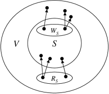
Figure 1: A subset (segment) $S$ and its corresponding read operands $R_{S}$, and write operands $W_{S}$.

3.3 Edge expansion and I/O-complexity 

Consider a segment $S$ and its read and write operands $R_{S}$ and $W_{S}$ (see Figure 1). If the graph $G$ containing $S$ has $h(G)$ edge expansion, maximum degree $d$ and at least $2|S|$ vertices, then (using the definition of $h(G)$), we have

Claim 2.

$|R_{S}|+|W_{S}|\geq\frac{1}{2}\cdot h(G)\cdot|S|$ .

Proof 3.1.

We have $|E(S,V\setminus S)|\geq h(G)\cdot d\cdot|S|$. Either (at least) half of the edges $E(S,V\setminus S)$ touch $R_{S}$ or half of them touch $W_{S}$. As every vertex is of degree $d$, we have $|R_{S}|+|W_{S}|\geq\max\{|R_{S}|,|W_{S}|\}\geq\frac{1}{d}\cdot\frac{1}{2}\cdot|E(S,V\setminus S)|\geq h(G)\cdot|S|/2$.

Combining this with (6) and choosing to partition $V$ into $|V|/s$ segments of equal size $s$, we obtain: $IO\geq\max_{s}\frac{|V|}{s}\cdot\left(\frac{h(G)\cdot s}{2}-2M\right)=\Omega\left(|V|\cdot h(G)\right)$. In many cases $h(G)$ is too small to attain the desired I/O-complexity lower bound. Typically, $h(G)$ is a decreasing function in $|V(G)|$, namely the edge expansion deteriorates with the increase of the input size and with the running time of the corresponding algorithm. This is the case with matrix multiplication algorithms: the cubic, as well as the Strassen and “Strassen-like” algorithms. In such cases, it is better to consider the expansion of $G$ on small sets only: $IO\geq\max_{s}\frac{|V|}{s}\cdot\left(\frac{h_{s}(G)\cdot s}{2}-2M\right)$. Choosing the minimal $s$ so that

$$\frac{h_{s}(G)\cdot s}{2}\geq 3M$$ (7)

we obtain

$$IO \geq \frac{|V|}{s}\cdot M~{}.$$ (8)

In some cases, the computation graph $G$ does not fit this analysis: it may not be regular, it may have vertices of unbounded degree, or its edge expansion may be hard to analyze. In such cases, we may consider some subgraph $G^{\prime}$ of $G$ instead to obtain a lower bound on the I/O-complexity :

Claim 3.

Let $G=(V,E)$ be a computation graph of an algorithm $Alg$. Let $G^{\prime}=(V^{\prime},E^{\prime})$ be a subgraph of $G$, i.e., $V^{\prime}\subseteq V$ and $E^{\prime}\subseteq E$. If $G^{\prime}$ is $d$-regular and $\alpha=\frac{|V^{\prime}|}{|V|}$, then the I/O-complexity of $Alg$ is

$$IO\geq\frac{\alpha}{2}\cdot\frac{|V|}{s}\cdot M$$ (9)

where $s$ is chosen so that ${h_{s}(G^{\prime})\cdot\alpha s\over 2}\geq 3M~{}$.

The correctness of this claim follows from Equations (7) and (8), and from the fact that at least an $\alpha/2$ fraction of the segments have at least $\frac{\alpha}{2}\cdot s$ of their vertices in $G^{\prime}$ (otherwise $V^{\prime}<\frac{\alpha}{2}\cdot V/s\cdot s+(1-\frac{\alpha}{2})\cdot V/s\cdot\frac{\alpha}{2}s<\alpha V$). We therefore have:

Lemma 3.2.

Let $Alg$ be an algorithm with $AO(N)$ arithmetic operations ($N$ being the total input size, $N=\Theta(n^{2})$ for matrix multiplication) and computation graph $G(N)=(V,E)$. Let $G^{\prime}(N)=(V^{\prime},E^{\prime})$ be a regular constant degree subgraph of $G$, with $\frac{|V^{\prime}|}{|V|}=\Theta(1)$. Then the I/O-complexity of $Alg$ on a machine with fast memory of size $M$ is

$$IO=\Omega\left(|V^{\prime}|\cdot h_{s}(G^{\prime}(N))\right)\;\;\text{ for}\;\;s=AO(M)~{}.$$ (10)

As $AO(N)=\Theta(|V^{\prime}|)$ and $h_{s}(G^{\prime}(N))$ for $s=AO(M)$ is $\Theta(h(G^{\prime}(M)))$ (recall Claim 1) we obtain, equivalently,

$$IO=\Omega\left(AO(N)\cdot h(G^{\prime}(M))\right)~{}.$$ (11)

4 Expansion Properties of Strassen’s Algorithm

Recall Strassen’s algorithm for matrix multiplication (see Algorithm 1 in Appendix A) and consider its computation graph (see Figure 2). Let $H_{i}$ be computation graph of Strassen’s algorithm for recursion of depth $i$, hence $H_{\lg n}$ corresponds to the computation for input matrices of size $n\times n$. $H_{\lg n}$ has the following structure:

• Encode $A$: generate weighted sums of elements of $A$ (this corresponds to the left factors of lines 5-11 of the algorithm).

• Similarly encode $B$ (this corresponds to the right factors of lines 5-11 of the algorithm).

• Then multiply the encodings of $A$ and $B$ element-wise (this corresponds to line 2 of the algorithm).

• Finally, decode $C$, by taking weighted sums of the products (this corresponds to lines 12-15 of the algorithm).

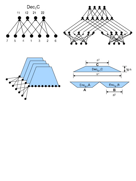
Figure 2: The computation graph of Strassen’s algorithm (See Algorithm 1 in Appendix).
Top left: $Dec_{1}C$. Top right: $H_{1}$. Bottom left: $Dec_{\lg n}C$. Bottom right: $H_{\lg n}$.

Comment 4.1

$Dec_{1}C$ is presented, for simplicity, with vertices of in-degree larger than two (but constant). A vertex of degree larger than two, in fact, represents a full binary (not necessarily balanced) tree. Note that replacing these high in-degree vertices with trees changes the edge expansion of the graph by a constant factor at most (as this graph is of constant size, and connected). Moreover, there is no change in the number of input and output vertices. Therefore the arguments in the following proof of Lemma 4.2 still hold.

4.1 The computation graph for $n$-by-$n$ matrices

Assume w.l.o.g. that $n$ is an integer power of $2$. Denote by $Enc_{\lg n}A$ the part of $H_{\lg n}$ that corresponds to the encoding of matrix $A$. Similarly, $Enc_{\lg n}B$, and $Dec_{\lg n}C$ correspond to the parts of $H_{\lg n}$ that compute the encoding of $B$ and the decoding of $C$, respectively.

4.1.1 A top-down construction of the computation graph

We next construct the computation graph $H_{i+1}$ by constructing $Dec_{i+1}C$ (from $Dec_{i}C$ and $Dec_{1}C$) and similarly constructing $Enc_{i+1}A$ and $Enc_{i+1}B$, then composing the three parts together.

• Duplicate $Dec_{1}C$ $7^{i}$ times.

• Duplicate $Dec_{i}C$ four times.

• Identify the $4\cdot 7^{i}$ output vertices of the copies of $Dec_{1}C$ with the $4\cdot 7^{i}$ input vertices of the copies of $Dec_{i}C$:

  • Recall that each $Dec_{1}C$ has four output vertices.

  • The first output vertex of the $7^{i}$ $Dec_{1}C$ graphs are identified with the $7^{i}$ input vertices of the first copy of $Dec_{i}C$.

  • The second output vertex of the $7^{i}$ $Dec_{1}C$ graphs are identified with the $7^{i}$ input vertices of the second copy of $Dec_{i}C$. And so on.

  • We make sure that the $j$th input vertex of a copy of $Dec_{i}C$ is identified with an output vertex of the $j$th copy of $Dec_{1}C$.

• We similarly obtain $Enc_{i+1}A$ from $Enc_{i}A$ and $Enc_{1}A$,

• and $Enc_{i+1}B$ from $Enc_{i}B$ and $Enc_{1}B$.

• For every $i$, $H_{i}$ is obtained by connecting edges from the $j$th output vertices of $Enc_{i}A$ and $Enc_{i}B$ to the $j$th input vertex of $Dec_{i}C$.

This completes the construction. Let us note some properties of these graphs.

The graph $Dec_{1}C$ has no vertices which are both input and output. As all out-degrees are at most 4 and all in degree are at most 2 (Recall Comment 4.1) we have:

Fact 4.

All vertices of $Dec_{\lg n}C$ are of degree at most $6$.

However, $Enc_{1}A$ and $Enc_{1}B$ have vertices which are both input and output (e.g., $A_{11}$), therefore $Enc_{\lg n}A$ and $Enc_{\lg n}B$ have vertices of out-degree $\Theta(\lg n)$. All in-degrees are at most $2$, as an arithmetic operation has at most two inputs.

As $H_{\lg n}$ contains vertices of large degrees, it is easier to consider $Dec_{\lg n}C$: it contains only vertices of constant bounded degree, yet at least one third of the vertices of $H_{\lg n}$ are in it.

Lemma 4.2.

(Main lemma) The edge expansion of $Dec_{k}C$ is

$$h(Dec_{k}C)=\Omega\left(\left(\frac{4}{7}\right)^{k}\right)$$

The proof follows below, but first note that it suffices to deduce the expansion of $Dec_{\lg n}C$ on small sets. Assume w.l.o.g. that $n$ is an integer power of $\sqrt{M}$. Then $Dec_{\lg n}C$ can be split into edge-disjoint copies of $Dec_{\frac{1}{2}\lg M}C$. Using Claim 1, we thus have:

Corollary 4.3.

$s\cdot h_{s}(Dec_{\lg n}C)\geq 3M$ for $s=9\cdot M^{\lg 7/2}$.

As $Dec_{\lg n}C$ contains $\alpha=\frac{1}{3}$ of the vertices of $H_{\lg n}$, Lemma 3.2 now yields Main Theorem 1.1. Note that $Dec_{\lg n}C$ has no input vertices, so no restriction on input replication is needed.

4.1.2 Combinatorial Estimation of the Expansion

Proof 4.4 (of Lemma 4.2).

Let $G_{k}=(V,E)$ be $Dec_{k}C$, and let $S\subseteq V,|S|\leq|V|/2$. We next show that $|E(S,V\setminus S)|\geq c\cdot d\cdot|S|\cdot\left(\frac{4}{7}\right)^{k}$, where $c$ is some universal constant, and $d$ is the constant degree of $Dec_{k}C$ (after adding loops to make it regular).

The proof works as follows. Recall that $G_{k}$ is a layered graph (with layers corresponding to recursion steps), so all edges (excluding loops) connect between consecutive levels of vertices. We argue (in Claim 8) that each level of $G_{k}$ contains about the same fraction of $S$ vertices, or else we have many edges leaving $S$. We also observe (in Fact 9) that such homogeneity (of a fraction of $S$ vertices) does not hold between distinct parts of the lowest level, or, again, we have many edges leaving $S$. We then show that the homogeneity between levels, combined with the heterogeneity of the lowest level, guarantees that there are many edges leaving $S$.

Let $l_{i}$ be the $i$th level of vertices of $G_{k}$, so $4^{k}=|l_{1}|<|l_{2}|<\cdots<|l_{i}|=4^{k-i+1}7^{i-1}<\cdots<|l_{k+1}|=7^{k}$. Let $S_{i}\equiv S\cap l_{i}$. Let $\sigma=\frac{|S|}{|V|}$ be the fractional size of $S$ and $\sigma_{i}=\frac{|S_{i}|}{|l_{i}|}$ be the fractional size of $S$ at level $i$. Due to averaging, we observe the following:

Fact 5.

There exist $i$ and $i^{\prime}$ such that $\sigma_{i}\leq\sigma\leq\sigma_{i^{\prime}}$.

Fact 6.

$$|V| = \sum_{i=1}^{k+1}|l_{i}|=\sum_{i=1}^{k+1}|l_{k+1}|\cdot\left(\frac{4}{7}\right)^{i}$$

$$= |l_{k+1}|\cdot\left(1-\left(\frac{4}{7}\right)^{k+2}\right)\cdot\frac{7}{3}$$

$$= \left(\frac{4}{7}\right)^{k}\cdot|l_{1}|\cdot\left(1-\left(\frac{4}{7}\right)^{k+2}\right)\cdot\frac{7}{3}$$

so $\frac{3}{7}\leq\frac{|l_{k+1}|}{|V|}\leq\frac{3}{7}\cdot\frac{1}{1-\left(\frac{4}{7}\right)^{k+2}}$, and $\frac{3}{7}\cdot\left(\frac{4}{7}\right)^{k}\leq\frac{|l_{1}|}{|V|}\leq\frac{3}{7}\cdot\left(\frac{4}{7}\right)^{k}\cdot\frac{1}{1-\left(\frac{4}{7}\right)^{k+2}}.$

Claim 7.

There exists $c^{\prime}=c^{\prime}(G_{1})$ so that $|E(S,V\setminus S)\cap E(l_{i},l_{i+1})|\geq c^{\prime}\cdot d\cdot|\delta_{i}|\cdot|l_{i}|$.

Proof 4.5.

Let $G^{\prime}$ be a $G_{1}$ component connecting $l_{i}$ with $l_{i+1}$ (so it has four vertices in $l_{i}$ and seven in $l_{i+1}$). $G^{\prime}$ has no edges in $E(S,V\setminus S)$ if all or none of its vertices are in $S$. Otherwise, as $G^{\prime}$ is connected, it contributes at least one edge to $E(S,V\setminus S)$. The number of such $G_{1}$ components with all their vertices in $S$ is at most $\min\{\sigma_{i},\sigma_{i+1}\}\cdot\frac{|l_{i}|}{4}$. Therefore, there are at least $|\sigma_{i}-\sigma_{i+1}|\cdot\frac{|l_{i}|}{4}$ $G_{1}$ components with at least one vertex in $S$ and one vertex that is not.

Claim 8 (Homogeneity between levels).

If there exists $i$ so that $\frac{|\sigma-\sigma_{i}|}{\sigma}\geq\frac{1}{10}$, then

$$|E(S,V\setminus S)|\geq c\cdot d\cdot|S|\cdot\left(\frac{4}{7}\right)^{k}$$

where $c>0$ is some constant depending on $G_{1}$ only.

Proof 4.6.

Assume that there exists $j$ so that $\frac{|\sigma-\sigma_{j}|}{\sigma}\geq\frac{1}{10}$. Let $\delta_{i}\equiv\sigma_{i+1}-\sigma_{i}$. By Claim 7, we have

$$|E(S,V\setminus S)| \geq \sum_{i\in[k]}|E(S,V\setminus S)\cap E(l_{i},l_{i+1})|$$

$$\geq \sum_{i\in[k]}c^{\prime}\cdot d\cdot|\delta_{i}|\cdot|l_{i}|$$

$$\geq c^{\prime}\cdot d\cdot|l_{1}|\sum_{i\in[k]}|\delta_{i}|$$

$$\geq c^{\prime}\cdot d\cdot|l_{1}|\cdot\left(\max_{i\in[k+1]}\sigma_{i}-\min_{i\in[k+1]}\sigma_{i}\right).$$

By the initial assumption, there exists $j$ so that $\frac{|\sigma-\sigma_{j}|}{\sigma}\geq\frac{1}{10}$, therefore $\max_{i}\sigma_{i}-\min_{i}\sigma_{i}\geq\frac{\sigma}{10}$, then

$$|E(S,V\setminus S)| \geq c^{\prime}\cdot d\cdot|l_{1}|\cdot\frac{\sigma}{10}$$

By Fact 6, $$|l_{1}|\geq\frac{3}{7}\cdot\left(\frac{4}{7}\right)^{k}\cdot|V|$$,

$$\geq c^{\prime}\cdot d\cdot\frac{3}{7}\cdot\left(\frac{4}{7}\right)^{k}\cdot|V|\cdot\frac{\sigma}{10}$$

As $$|S|=\sigma\cdot|V|$$,

$$\geq c\cdot d\cdot|S|\cdot\left(\frac{4}{7}\right)^{k}$$

for any $c\leq\frac{c^{\prime}}{10}\cdot\frac{3}{7}$.

Let $T_{k}$ be a tree corresponding to the recursive construction of $G_{k}$ in the following way (see Figure 3): $T_{k}$ is a tree of height $k+1$, where each internal node has four children. The root $r$ of $T_{k}$ corresponds to $l_{k+1}$ (the largest level of $G_{k}$). The four children of $r$ correspond to the largest levels of the four graphs that one can obtain by removing the level of vertices $l_{k+1}$ from $G_{k}$. And so on. For every node $u$ of $T_{k}$, denote by $V_{u}$ the set of vertices in $G_{k}$ corresponding to $u$. We thus have $|V_{r}|=7^{k}$ where $r$ is the root of $T_{k}$, $|V_{u}|=7^{k-1}$ for each node $u$ that is a child of $r$; and in general we have $4^{i}$ tree nodes $u$ corresponding to a set of size $|V_{u}|=7^{k-i+1}$. Each leaf $l$ corresponds to a set of size $1$.

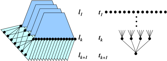
Figure 3: The graph $G_{k}$ and its corresponding tree $T_{k}$.

For a tree node $u$, let us define $\rho_{u}=\frac{|S\cap V_{u}|}{|V_{u}|}$ to be the fraction of $S$ nodes in $V_{u}$, and $\delta_{u}=|\rho_{u}-\rho_{p(u)}|$, where $p(u)$ is the parent of $u$ (for the root $r$ we let $p(r)=r$). We let $t_{i}$ be the $i$th level of $T_{k}$, counting from the bottom, so $t_{k+1}$ is the root and $t_{1}$ are the leaves.

Fact 9.

As $V_{r}=l_{k+1}$ we have $\rho_{r}=\sigma_{k+1}$. For a tree leaf $u\in t_{1}$, we have $|V_{u}|=1$. Therefore $\rho_{u}\in\{0,1\}$. The number of vertices $u$ in $t_{1}$ with $\rho_{u}=1$ is $\sigma_{1}\cdot|l_{1}|$.

Claim 10.

Let $u_{0}$ be an internal tree node, and let $u_{1},u_{2},u_{3},u_{4}$ be its four children. Then

$$\sum_{i}|E(S,V\setminus S)\cap E(V_{u_{i}},V_{u_{0}})|\geq c^{\prime\prime}\cdot d\cdot\sum_{i}|\rho_{u_{i}}-\rho_{u_{0}}|\cdot|V_{u_{i}}|$$

where $c^{\prime\prime}=c^{\prime\prime}(G_{1})$.

Proof 4.7.

The proof follows that of Claim 7. Let $G^{\prime}$ be a $G_{1}$ component connecting $V_{u_{0}}$ with $\bigcup_{i\in[4]}V_{u_{i}}$ (so it has seven vertices in $V_{u_{0}}$ and one in each of $V_{u_{1}}$,$V_{u_{2}}$,$V_{u_{3}}$,$V_{u_{4}}$). $G^{\prime}$ has no edges in $E(S,V\setminus S)$ if all or none of its vertices are in $S$. Otherwise, as $G^{\prime}$ is connected, it contributes at least one edge to $E(S,V\setminus S)$. The number of $G_{1}$ components with all their vertices in $S$ is at most $\min\{\rho_{u_{0}},\rho_{u_{1}},\rho_{u_{2}},\rho_{u_{3}},\rho_{u_{4}}\}\cdot\frac{|V_{u_{1}}|}{4}$. Therefore, there are at least $\max_{i\in[4]}\{|\rho_{u_{0}}-\rho_{u_{i}}|\}\cdot\frac{|V_{u_{1}}|}{4}\geq\frac{1}{16}\cdot\sum_{i\in[4]}|\rho_{u_{i}}-\rho_{u_{0}}|\cdot|V_{u_{i}}|$   $G_{1}$ components with at least one vertex in $S$ and one vertex that is not.

We have

$$|E(S,V\setminus S)| =\sum_{u\in T_{k}}|E(S,V\setminus S)\cap E(V_{u},V_{p(u)})|$$

By Claim 10, this is

$$\geq\sum_{u\in T_{k}}c^{\prime\prime}\cdot d\cdot|\rho_{u}-\rho_{p(u)}|\cdot|V_{u}|$$

$$=c^{\prime\prime}\cdot d\cdot\sum_{i\in[k]}\sum_{u\in t_{i}}|\rho_{u}-\rho_{p(u)}|\cdot 7^{i-1}$$

$$\geq c^{\prime\prime}\cdot d\cdot\sum_{i\in[k]}\sum_{u\in t_{i}}|\rho_{u}-\rho_{p(u)}|\cdot 4^{i-1}$$

As each internal node has four children, this is

$$=c^{\prime\prime}\cdot d\cdot\sum_{v\in t_{1}}\sum_{u\in v\sim r}|\rho_{u}-\rho_{p(u)}|$$

where $$v\sim r v r |~{}\cdot~{}|$$ is the path from to the root . By the triangle inequality for the function 

$$\geq c^{\prime\prime}\cdot d\cdot\sum_{v\in t_{1}}|\rho_{u}-\rho_{r}|$$

By Fact 9,

$$\geq c^{\prime\prime}\cdot d\cdot|l_{1}|\cdot((1-\sigma_{1})\cdot\rho_{r}+\sigma_{1}\cdot(1-\rho_{r}))$$

By Claim 8, w.l.o.g., $$|\sigma_{k+1}-\sigma|/\sigma\leq\frac{1}{10} |\sigma_{1}-\sigma|/\sigma\leq\frac{1}{10} \rho_{r}=\sigma_{k+1}$$ and . As ,

$$\geq\frac{3}{4}\cdot c^{\prime\prime}\cdot d\cdot|l_{1}|\cdot\sigma$$

and by Fact 6,

$$\geq c\cdot d\cdot|S|\cdot\left(\frac{4}{7}\right)^{k}$$

for any $$c\leq\frac{3}{4}\cdot c^{\prime\prime}$$.

This completes the proof of Lemma 4.2.

5 Other Algorithms

We now discuss the applicability of our approach to other algorithms, starting with other fast matrix multiplication algorithms.

5.1 “Strassen-like” Algorithms

A “Strassen-like” algorithm has a recursive structure that utilizes a base case: multiplying two $n_{0}$-by-$n_{0}$ matrices using $m(n_{0})$ multiplications. Given two matrices of size $n$-by-$n$, it splits them into $n_{0}^{2}$ blocks (each of size $\frac{n}{n_{0}}$-by-$\frac{n}{n_{0}}$), and works blockwise, according to the base case algorithm. Additions (and subtractions) in the base case are interpreted as additions (and subtractions) of blocks. These are performed element-wise. Multiplications in the base case are interpreted as multiplications of blocks. These are performed by recursively calling the algorithm. The arithmetic count of the algorithm is then $T(n)=m(n_{0})\cdot T\left(\frac{n}{n_{0}}\right)+O(n^{2})$, so $T(n)=\Theta(n^{\omega_{0}})$ where $\omega_{0}=\log_{n_{0}}m(n_{0})$.

This is the structure of all the fast matrix multiplication algorithms that were obtained since Strassen’s [Pan (1980), Bini (1980), Schönhage (1981), Romani (1982), Coppersmith and Winograd (1982), Strassen (1987), Coppersmith and Winograd (1987)], (see [Bűrgisser et al. (1997)] for discussion of these algorithms), as well as [Cohn et al. (2005)], where the base case utilizes a novel group-theoretic approach. In fact, any fast matrix multiplication algorithm can be converted into this form [Raz (2003)], and can even be made numerically stable while preserving this form [Demmel, Dumitriu, Holtz, and Kleinberg, 2007].

5.1.1 A critical technical assumption

For our technique to work, we further demand that the $Dec_{1}C$ part of the computation graph is a connected graph, in order to be “Strassen-like” (this was assumed in the proof of Claim 7). Thus the “Strassen-like” class includes Winograd’s variant of Strassen’s algorithm [Winograd (1971)], which uses 15 additions rather than 18, but not the cubic algorithm, where $Dec_{1}C$ is composed of four disconnected graphs (corresponding to the four outputs). We conjecture that $Dec_{1}C$ is indeed connected for all existing fast matrix-multiplication algorithms. We note that the demand of connectivity of $Dec_{1}C$ may be waved in some cases (see [Ballard et al. (2011e)]).

5.1.2 The communication costs of “Strassen-like” algorithms

To prove Theorem 1.3, which generalizes the I/O-complexity lower bound of Strassen’s algorithm (Theorem 1.1) to all “Strassen-like” algorithms, we note the following: The entire proof of Theorem 1.1, and in particular, the computations in the proof of Lemma 4.2, hold for any “Strassen-like” algorithm, where we plug in $n_{0}^{2},m(n_{0})$, and $\frac{n_{0}}{m(n_{0})}$ instead of $4,7$, and $\frac{4}{7}$. For bounding the asymptotic I/O-complexity , we do not care about the number of internal vertices of $Dec_{1}C$; we need only to know that $Dec_{1}C$ is connected (this critical technical assumption is used in the proof of Claim 7), and to know the sizes $n_{0}$ and $m(n_{0})$. The only nontrivial adjustment is to show the equivalent of Fact 4: that the graph $Dec_{\log n}C$ is of bounded degree.

Claim 11.

The $Dec_{\log n}C$ graph of any “Strassen-like” algorithm is of degree bounded by a constant.

Proof 5.1.

If the set of input vertices of $Dec_{1}C$, and the set of its output vertices are disjoint, then $Dec_{\log n}C$ is of constant bounded degree (its maximal degree is at most twice the largest degree of $Dec_{1}C$).

Assume (towards contradiction) that the base graph $Dec_{1}C$ has an input vertex which is also an output vertex. An output vertex represents the inner product of two $n_{0}$-long vectors, i.e., the corresponding row-vector of $A$ and column vector of $B$. The corresponding bilinear polynomial is irreducible. This is a contradiction, since an input vertex represents the multiplication of a (weighted) sum of elements of $A$ with a (weighted) sum of elements of $B$.

5.2 Uniform, Non-stationary Fast Matrix Multiplication Algorithms

Another class of matrix multiplication algorithms, the uniform, non-stationary algorithms, allows mixing of schemes of the previous (“Strassen-like”) class. In each recursive level, a different scheme may be used. The CDAG has a repeating structure inside one level, but the structure may differ between two distinct levels. This class includes, for example, algorithms that optimize for input sizes (for sizes that are not an integer power of a constant integer). The class also includes algorithms that cut the recursion off at some point, and then switch to the classical algorithm. For these and other implementation issues, see [Douglas et al. (1994), Huss-Lederman et al. (1996)] (sequential model) and [Desprez and Suter (2004)] (parallel model). The I/O-complexity lower bound generalizes to this class, and will appear in a separate note [Ballard et al. (2011e)].

5.3 Non-uniform, Non-stationary Fast Matrix Multiplication Algorithms

A third class, the non-uniform, non-stationary algorithms, allows recursive calls to have different structure, even when they refer to multiplication of matrices in the same recursive level. It is not clear how to analyze the expansion of the CDAG of an algorithm in the third class, although we are not aware of any algorithms in this class. Such an analysis, applied to the base case of [Cohn et al. (2005)], may improve the I/O-complexity lower bound for fast matrix multiplication by a (large) constant.

5.4 Multiplying Rectangular Matrices

Multiplication of rectangular matrices have seen a series of increasingly fast algorithms culminating in Coppersmith’s algorithm [Coppersmith (1997)]. It is possible to extend our approach and obtain the first lower bounds on the communication costs for these algorithms, and show that in some cases they are attainable, and therefore optimal [Ballard et al. (2011d)].

5.5 Other Algorithms

Fast matrix multiplication algorithms are basic building blocks in many fast algorithms in linear algebra, such as algorithms for LU, QR, and solving the Sylvester equation [Demmel, Dumitriu, and Holtz, 2007]. Therefore, I/O-complexity lower bounds for these algorithms can be derived from our lower bounds for fast matrix multiplication algorithms [Ballard et al. (2011a)]. For example, a lower bound on LU (or QR, etc.) follows when the fast matrix multiplication algorithm is called by the LU algorithm on sufficiently large subblocks of the matrix. This is the case in the algorithms of [Demmel, Dumitriu, and Holtz, 2007], and we can then deduce matching lower and upper bounds [Ballard et al. (2011a)].

6 Conclusions and Open Problems

We obtained a tight lower bound for the I/O-complexity of Strassen’s and “Strassen-like” fast matrix multiplication algorithms. These bounds are optimal for the sequential model with two memory levels and with memory hierarchy. The lower bounds extend to the parallel model and other models. Recently these bounds were attained (up to an $O(\log p)$ factor) by new parallel implementations, for Strassen’s algorithm and for “Strassen-like” algorithms [Ballard et al. (2011)].

6.1 Memory constraints for the classical and “Strassen-like” matrix multiplication algorithms

Some (parallel) algorithms require very little, up to a constant factor extra memory beyond what is necessary to keep the input and output. These are sometimes called linear space algorithms. One class of such algorithms are the “2D” algorithms for classical matrix multiplication, that use two-dimensional grid of processors. Here we allow $M=\Theta\left(\frac{n^{2}}{p}\right)$ local memory use (recall that $p$ is the number of processors, and $n$ the dimension of the matrices), thus no replication of the input matrices is allowed [Cannon (1969)].

If the underlying grid of $p$ processors is a three-dimensional mesh, and the available memory per processor is larger by a factor of $p^{\frac{1}{3}}$ than the minimum necessary to store the input and output matrices, then a “3D” algorithm can be used (see [Dekel et al. (1981), Aggarwal et al. (1990), Agarwal et al. (1995), McColl and Tiskin (1999)]). These “3D” algorithms can reduce the communication cost by a factor of $p^{1/6}$, down to $\Theta\left(\frac{n^{2}}{p^{\frac{2}{3}}}\right)$ [Aggarwal et al. (1990)], attaining the lower bounds [Irony et al. (2004), Ballard et al. (2011c)] that take into account any amount of replication.

Recently, Demmel and Solomonik [Solomonik and Demmel (2011)] showed how to combine these two extremes into one algorithm (named “2.5D”) and obtained a communication efficient implementation for classical matrix multiplication, for local memory size $M=\Theta\left(c\cdot\frac{n^{2}}{p}\right)$ for any $1\leq c\leq p^{\frac{1}{3}}$. See Table 1.

Using Corollaries 1.2 and 1.4, and plugging in $M=\Theta\left(\frac{n^{2}}{p}\right)$, $M=\Theta\left(\frac{n^{2}}{p^{\frac{2}{3}}}\right)$ , and $M=\Theta\left(c\cdot\frac{n^{2}}{p}\right)$ we obtain corresponding lower bounds for “Strassen-like” algorithm with various restriction local memory sizes. These were recently attained by a new parallel implementation for Strassen and “Strassen-like” algorithms [Ballard et al. (2011)] (see Table 1). Interestingly, the numerators here do not depend on $\omega_{0}$. Thus, an improvement of $\omega_{0}$ (the exponent of the arithmetic cost of the algorithm) affects only the power of $p$ in the denominator.

	Classical algorithms		“Strassen-like” algorithms
			$2<\omega_{0}<3$
	Lower bound	Attained by	Lower bound	Attained by
Parallel	[Irony et al. (2004)]		[here]
$M=$	$\Omega\left(\left(\frac{n}{\sqrt{M}}\right)^{3}\cdot\frac{M}{p}\right)$		$\Omega\left(\left(\frac{n}{\sqrt{M}}\right)^{\omega_{0}}\cdot\frac{M}{p}\right)$
$\;\;\;\;\Theta\left(\frac{n^{2}}{p}\right)$	$\Omega\left(\frac{n^{2}}{p^{\frac{1}{2}}}\right)$	[Cannon (1969)]	$\Omega\left(\frac{n^{2}}{p^{2-\frac{\omega_{0}}{2}}}\right)$	[Ballard,
				Demmel,
$\;\;\;\;\Theta\left(\frac{n^{2}}{p^{\frac{2}{3}}}\right)$	$\Omega\left(\frac{n^{2}}{p^{\frac{2}{3}}}\right)$	[Dekel et al. (1981)]	$\Omega\left(\frac{n^{2}}{p^{\frac{5-\omega_{0}}{3}}}\right)$	Holtz,
		[Aggarwal et al. (1990)]		Rom,
$\;\;\;\;\Theta\left(c\cdot\frac{n^{2}}{p}\right)$	$\left(\frac{n^{2}}{c^{\frac{1}{2}}p^{\frac{1}{2}}}\right)$	[Solomonik and	$\Omega\left(\frac{n^{2}}{c^{\frac{\omega_{0}}{2}-1}p^{2-\frac{\omega_{0}}{2}}}\right)$	Schwartz,
$1\leq c\leq p^{\frac{1}{3}}$		Demmel 2011]		2011]

Table 1:

6.2 Recursive Implementations

In some cases, the simplest recursive implementation of an algorithm turns out to be communication-optimal (e.g., in the cases of matrix multiplication [Frigo et al. (1999)] and Cholesky decomposition [Ahmed and Pingali (2000), Ballard et al. (2010)], but not in the case of LU decomposition [Toledo (1997)], which is bandwidth optimal but not latency optimal). This leads to the question: when is the communication-optimality of an algorithm determined by the expansion properties of the corresponding computation graphs? In this work we showed that such is the case for “Strassen-like” fast matrix multiplication algorithms.

6.3 Other Hardware

It is of great interest to construct new models general enough to capture the rich and evolving design space of current and predicted future computers. Such models can be homogeneous, consisting of many layers, where the components of each layer are the same (e.g., a supercomputer with many identical multi-core chips on a board, many identical boards in a rack, many identical racks, and many identical levels of associated memory hierarchy); or heterogeneous, with components with different properties residing on the same level (e.g., CPUs alongside GPUs, where the latter can do some computations very quickly, but are much slower to communicate with).

Some experience has been acquired with such systems (see the MAGMA project [(7)], and also [Volkov and Demmel (2008)] for using GPU assisted linear algebra computation ). A first step in analyzing such systems has been recently introduced by Ballard, Demmel, and Gearhart [Ballard et al. (2011)], where they modeled heterogenous shared memory architectures, such as mixed GPU/CPU architecture, and obtained tight lower and upper bounds for $O(n^{3})$ matrix multiplication.

Note that we can similarly generalize Corollaries 1.2 and 1.4 to other models, such as the heterogenous model and shared memory model. The reduction is achieved by observing the communication of a single processor.

However, there is currently no systematic theoretic way of obtaining upper and lower bounds for arbitrary hardware models. Expanding such results to other architectures and algorithmic techniques is a challenging goal. For example, recursive algorithms tend to be cache oblivious and communication optimal for the sequential hierarchy model. Finding an equivalent technique that would work for an arbitrary architecture is a fundamental open problem.

We thank Eran Rom, Edgar Solomonik, and Chris Umans for helpful discussions.

Appendix A Strassen’s Fast Matrix Multiplication Algorithm

Strassen’s original algorithm follows [Strassen (1969)]. See [Winograd (1971)] for Winograd’s variant, which reduces the number of additions.

Algorithm 1 Matrix Multiplication: Strassen’s Algorithm

0:  Two $n\times n$ matrices, $A$ and $B$.

1:  if $n=1$ then

2:     $C_{11}=A_{11}\cdot B_{11}$

3:  else

4:     {Decompose $A$ into four equal square blocks $A=\begin{pmatrix}A_{11}&A_{12}\\ A_{21}&A_{22}\end{pmatrix}$ and the same for $B$.}

5:     $M_{1}=(A_{11}+A_{22})\cdot(B_{11}+B_{22})$

6:     $M_{2}=(A_{21}+A_{22})\cdot B_{11}$

7:     $M_{3}=A_{11}\cdot(B_{12}-B_{22})$

8:     $M_{4}=A_{22}\cdot(B_{21}-B_{11})$

9:     $M_{5}=(A_{11}+A_{12})\cdot B_{22}$

10:     $M_{6}=(A_{21}-A_{11})\cdot(B_{11}+B_{12})$

11:     $M_{7}=(A_{12}-A_{22})\cdot(B_{21}+B_{22})$

12:     $C_{11}=M_{1}+M_{4}-M_{5}+M_{7}$

13:     $C_{12}=M_{3}+M_{5}$

14:     $C_{21}=M_{2}+M_{4}$

15:     $C_{22}=M_{1}-M_{2}+M_{3}+M_{6}$

16:  end if

17:  return  $C$

References

- Agarwal et al. (1995) Agarwal, R. C., Balle, S. M., Gustavson, F. G., Joshi, M., and Palkar, P. 1995. A three-dimensional approach to parallel matrix multiplication. IBM Journal of Research and Development 39, 39–5.
- Aggarwal et al. (1990) Aggarwal, A., Chandra, A. K., and Snir, M. 1990. Communication complexity of PRAMs. Theor. Comput. Sci. 71, 3–28.
- Aggarwal and Vitter (1988) Aggarwal, A. and Vitter, J. S. 1988. The input/output complexity of sorting and related problems. Commun. ACM 31, 9, 1116–1127.
- Ahmed and Pingali (2000) Ahmed, N. and Pingali, K. 2000. Automatic generation of block-recursive codes. In Euro-Par ’00: Proceedings from the 6th International Euro-Par Conference on Parallel Processing. Springer-Verlag, London, UK, 368–378.
- Alon et al. (2008) Alon, N., Schwartz, O., and Shapira, A. 2008. An elementary construction of constant-degree expanders. Combinatorics, Probability & Computing 17, 3, 319–327.
- Anderson et al. (1992) Anderson, E., Bai, Z., Bischof, C., Demmel, J., Dongarra, J., Croz, J. D., Greenbaum, A., Hammarling, S., McKenney, A., Ostrouchov, S., and Sorensen, D. 1992. LAPACK’s user’s guide. Society for Industrial and Applied Mathematics, Philadelphia, PA, USA. Also available from http://www.netlib.org/lapack/.
- (7) Baboulin, M., Demmel, J., Dong, T., Dongarra, J., Horton, M., Jia, Y., Kabir, K., Langou, J., Li, Y., Ltaief, H., Nath, R., Tomov, S., and Volkov, V. The magma project. University of Tennessee, Department of Electrical Engineering and Computer Science. http://icl.cs.utk.edu/magma/.
- Ballard et al. (2011) Ballard, G., Demmel, J., and Dumitriu, I. 2011. Communication-optimal parallel and sequential eigenvalue and singular value algorithms. EECS Technical Report EECS-2011-14, UC Berkeley. Feb.
- Ballard et al. (2011) Ballard, G., Demmel, J., and Gearhart, A. 2011. Communication bounds for heterogeneous architectures. In 23rd ACM Symposium on Parallelism in Algorithms and Architectures (SPAA 2011). (‘brief announcement”).
- Ballard et al. (2011) Ballard, G., Demmel, J., Holtz, O., Rom, E., and Schwartz, O. 2011. Communication-Minimizing Parallel Implementation for Strassen’s Algorithm. Unpublished.
- Ballard et al. (2009) Ballard, G., Demmel, J., Holtz, O., and Schwartz, O. 2009. Communication-optimal Parallel and Sequential Cholesky Decomposition. In SPAA ’09: Proceedings of the twenty-first annual symposium on Parallelism in algorithms and architectures. ACM, New York, NY, USA, 245–252.
- Ballard et al. (2010) Ballard, G., Demmel, J., Holtz, O., and Schwartz, O. 2010. Communication-optimal parallel and sequential Cholesky decomposition. SIAM Journal on Scientific Computing 32, 6, 3495–3523.
- Ballard et al. (2011a) Ballard, G., Demmel, J., Holtz, O., and Schwartz, O. 2011a. Communication Cost of “Fast Linear Algebra is Stable” Algorithms. Unpublished.
- Ballard et al. (2011b) Ballard, G., Demmel, J., Holtz, O., and Schwartz, O. 2011b. Graph Expansion and Communication Costs of Fast Matrix Multiplication. In SPAA ’11: Proceedings of the 23rd annual symposium on parallelism in algorithms and architectures. ACM, New York, NY, USA, 1–12.
- Ballard et al. (2011c) Ballard, G., Demmel, J., Holtz, O., and Schwartz, O. 2011c. Minimizing communication in numerical linear algebra. SIAM Journal on Matrix Analysis and Applications. Accepted. Available from http://arxiv.org/abs/0905.2485.
- Ballard et al. (2011d) Ballard, G., Demmel, J., Holtz, O., and Schwartz, O. 2011d. Revisiting Coppersmith’s “Rectangular matrix multiplication revisited” for I/O-Complexity. Unpublished.
- Ballard et al. (2011e) Ballard, G., Demmel, J., Holtz, O., and Schwartz, O. 2011e. The Communication Costs of Hybrid Algorithms for Fast Matrix Multiplication. Unpublished.
- Bender et al. (2007) Bender, M. A., Brodal, G. S., Fagerberg, R., Jacob, R., and Vicari, E. 2007. Optimal sparse matrix dense vector multiplication in the I/O-model. In SPAA ’07: Proceedings of the nineteenth annual ACM symposium on Parallel algorithms and architectures. ACM, New York, NY, USA, 61–70.
- Bilardi et al. (2000) Bilardi, G., Pietracaprina, A., and D’Alberto, P. 2000. On the space and access complexity of computation DAGs. In WG ’00: Proceedings of the 26th International Workshop on Graph-Theoretic Concepts in Computer Science. Springer-Verlag, London, UK, 47–58.
- Bilardi and Preparata (1999) Bilardi, G. and Preparata, F. 1999. Processor-time tradeoffs under bounded-speed message propagation: Part II, lower boundes. Theory of Computing Systems 32, 5, 1432–4350.
- Bini (1980) Bini, D. 1980. Relations between exact and approximate bilinear algorithms. applications. Calcolo 17, 87–97. 10.1007/BF02575865.
- Blackford et al. (1997) Blackford, L. S., Choi, J., Cleary, A., D Azevedo, E., Demmel, J., Dhillon, I., Dongarra, J., Hammarling, S., Henry, G., Petitet, A., Stanley, K., Walker, D., and Whaley, R. C. 1997. ScaLAPACK Users’ Guide. SIAM, Philadelphia, PA, USA. Also available from http://www.netlib.org/scalapack/.
- Blelloch et al. (2008) Blelloch, G. E., Chowdhury, R. A., Gibbons, P. B., Ramachandran, V., Chen, S., and Kozuch, M. 2008. Provably good multicore cache performance for divide-and-conquer algorithms. In SODA ’08: Proceedings of the nineteenth annual ACM-SIAM symposium on Discrete algorithms. Society for Industrial and Applied Mathematics, Philadelphia, PA, USA, 501–510.
- Burago and Zalgaller (1988) Burago, Y. D. and Zalgaller, V. A. 1988. Geometric Inequalities. Grundlehren der Mathematische Wissenschaften Series, vol. 285. Springer, Berlin.
- Bűrgisser et al. (1997) Bűrgisser, P., Clausen, M., and Shokrollahi, M. A. 1997. Algebraic Complexity Theory. Number 315 in Grundlehren der mathematischen Wissenschaften. Springer Verlag.
- Cannon (1969) Cannon, L. 1969. A cellular computer to implement the kalman filter algorithm. Ph.D. thesis, Montana State University, Bozeman, MN.
- Chowdhury and Ramachandran (2006) Chowdhury, R. A. and Ramachandran, V. 2006. Cache-oblivious dynamic programming. In SODA ’06: Proceedings of the seventeenth annual ACM-SIAM symposium on Discrete algorithm. ACM, New York, NY, USA, 591–600.
- Cohn et al. (2005) Cohn, H., Kleinberg, R. D., Szegedy, B., and Umans, C. 2005. Group-theoretic algorithms for matrix multiplication. In FOCS. 379–388.
- Coppersmith (1997) Coppersmith, D. 1997. Rectangular matrix multiplication revisited. J. Complex. 13, 42–49.
- Coppersmith and Winograd (1982) Coppersmith, D. and Winograd, S. 1982. On the asymptotic complexity of matrix multiplication. SIAM Journal on Computing 11, 3, 472–492.
- Coppersmith and Winograd (1987) Coppersmith, D. and Winograd, S. 1987. Matrix multiplication via arithmetic progressions. In Proceedings of the nineteenth annual ACM symposium on Theory of computing. STOC ’87. ACM, New York, NY, USA, 1–6.
- Coppersmith and Winograd (1990) Coppersmith, D. and Winograd, S. 1990. Matrix multiplication via arithmetic progressions. J. Symb. Comput. 9, 3, 251–280.
- David et al. (2010) David, P.-Y., Demmel, J., Grigori, L., and Peyronnet, S. 2010. Brief announcement: Lower bounds on communication for sparse Cholesky factorization of a model problem. In 22nd ACM Symposium on Parallelism in Algorithms and Architectures (SPAA).
- Dekel et al. (1981) Dekel, E., Nassimi, D., and Sahni, S. 1981. Parallel matrix and graph algorithms. SIAM J. Comput., 657–675.
- Demmel et al. (2010) Demmel, J., Grigori, L., and Xiang, H. 2010. CALU: A communication optimal LU factorization algorithm. EECS Technical Report EECS-2010-29, UC Berkeley. Mar. Submitted to SIAM J. Matrix Anal. Appl.
- Desprez and Suter (2004) Desprez, F. and Suter, F. 2004. Impact of mixed-parallelism on parallel implementations of the Strassen and Winograd matrix multiplication algorithms: Research articles. Concurrency and Computation: Practice and Experience 16, 8, 771–797.
- Douglas et al. (1994) Douglas, C. C., Heroux, M., Slishman, G., and Smith, R. M. 1994. GEMMW: A portable level 3 BLAS Winograd variant of Strassen’s matrix-matrix multiply algorithm. Journal of Computational Physics 110, 1, 1–10.
- Elmroth and Gustavson (1998) Elmroth, E. and Gustavson, F. 1998. New serial and parallel recursive QR factorization algorithms for SMP systems. In Applied Parallel Computing. Large Scale Scientific and Industrial Problems., B. K. et al., Ed. Lecture Notes in Computer Science Series, vol. 1541. Springer, 120–128.
- Frens and Wise (2003) Frens, J. D. and Wise, D. S. 2003. QR factorization with Morton-ordered quadtree matrices for memory re-use and parallelism. SIGPLAN Not. 38, 10, 144–154.
- Frigo et al. (1999) Frigo, M., Leiserson, C. E., Prokop, H., and Ramachandran, S. 1999. Cache-oblivious algorithms. In FOCS ’99: Proceedings of the 40th Annual Symposium on Foundations of Computer Science. IEEE Computer Society, Washington, DC, USA, 285.
- Fuller and Millett (2011) Fuller, S. H. and Millett, L. I., Eds. 2011. The Future of Computing Performance: Game Over or Next Level? The national academies press, Washington, D.C. 200 pages, http://www.nap.edu.
- Graham et al. (2004) Graham, S. L., Snir, M., and Patterson, C. A., Eds. 2004. Getting up to Speed: The Future of Supercomputing. Report of National Research Council of the National Academies Sciences. The National Academies Press, Washington, D.C. 289 pages, http://www.nap.edu.
- Gustavson (1997) Gustavson, F. G. 1997. Recursion leads to automatic variable blocking for dense linear-algebra algorithms. IBM J. Res. Dev. 41, 6, 737–756.
- Hong and Kung (1981) Hong, J. W. and Kung, H. T. 1981. I/O complexity: The red-blue pebble game. In STOC ’81: Proceedings of the thirteenth annual ACM symposium on Theory of computing. ACM, New York, NY, USA, 326–333.
- Huss-Lederman et al. (1996) Huss-Lederman, S., Jacobson, E. M., Johnson, J. R., Tsao, A., and Turnbull, T. 1996. Implementation of Strassen’s algorithm for matrix multiplication. In Supercomputing ’96: Proceedings of the 1996 ACM/IEEE conference on Supercomputing (CDROM). IEEE Computer Society, Washington, DC, USA, 32.
- Irony et al. (2004) Irony, D., Toledo, S., and Tiskin, A. 2004. Communication lower bounds for distributed-memory matrix multiplication. J. Parallel Distrib. Comput. 64, 9, 1017–1026.
- Koucky et al. (2010) Koucky, M., Kabanets, V., and Kolokolova, A. 2010. Expanders made elementary. In preparation, Available from http://www.cs.sfu.ca/kabanets/papers/expanders.pdf.
- Leiserson (2008) Leiserson, C. E. 2008. Personal communication with G. Ballard, J. Demmel, O. Holtz, and O. Schwartz.
- Lev and Valiant (1983) Lev, G. and Valiant, L. G. 1983. Size bounds for superconcentrators. Theoretical Computer Science 22, 3, 233–251.
- Loomis and Whitney (1949) Loomis, L. H. and Whitney, H. 1949. An inequality related to the isoperimetric inequality. Bulletin of the AMS 55, 961–962.
- McColl and Tiskin (1999) McColl, W. F. and Tiskin, A. 1999. Memory-efficient matrix multiplication in the bsp model. Algorithmica 24, 287–297. 10.1007/PL00008264.
- Michael et al. (2002) Michael, J. P., Penner, M., and Prasanna, V. K. 2002. Optimizing graph algorithms for improved cache performance. In Proc. Int’l Parallel and Distributed Processing Symp. (IPDPS 2002), Fort Lauderdale, FL. 769–782.
- Mihail (1989) Mihail, M. 1989. Conductance and convergence of Markov chains: A combinatorial treatment of expanders. In Proceedings of the Thirtieth Annual IEEE Symposium on Foundations of Computer Science. 526– 531.
- Pan (1980) Pan, V. Y. 1980. New fast algorithms for matrix operations. SIAM Journal on Computing 9, 2, 321–342.
- Raz (2003) Raz, R. 2003. On the complexity of matrix product. SIAM J. Comput. 32, 5, 1356–1369 (electronic).
- Reingold et al. (2002) Reingold, O., Vadhan, S., and Wigderson, A. 2002. Entropy waves, the zig-zag graph product, and new constant-degree expanders. Annals of Mathematics 155, 1, 157–187.
- Romani (1982) Romani, F. 1982. Some properties of disjoint sums of tensors related to matrix multiplication. SIAM Journal on Computing 11, 2, 263–267.
- Savage (1994) Savage, J. 1994. Space-time tradeoffs in memory hierarchies. Tech. rep., Brown University, Providence, RI, USA.
- Schönhage (1981) Schönhage, A. 1981. Partial and total matrix multiplication. SIAM Journal on Computing 10, 3, 434–455.
- Solomonik and Demmel (2011) Solomonik, E. and Demmel, J. 2011. Communication-optimal parallel 2.5D matrix multiplication and LU factorization algorithms. In Euro-Par’11: Proceedings of the 17th International European Conference on Parallel and Distributed Computing. Springer.
- Strassen (1969) Strassen, V. 1969. Gaussian elimination is not optimal. Numer. Math. 13, 354–356.
- Strassen (1987) Strassen, V. 1987. Relative bilinear complexity and matrix multiplication. Journal fűr die reine und angewandte Mathematik (Crelles Journal) 1987, 375–376, 406–443.
- Toledo (1997) Toledo, S. 1997. Locality of reference in LU decomposition with partial pivoting. SIAM J. Matrix Anal. Appl. 18, 4, 1065–1081.
- Volkov and Demmel (2008) Volkov, V. and Demmel, J. 2008. Benchmarking GPUs to tune dense linear algebra. In SC ’08: Proceedings of the 2008 ACM/IEEE conference on Supercomputing. IEEE Press, Piscataway, NJ, USA, 1–11.
- Winograd (1971) Winograd, S. 1971. On the multiplication of 2 2 matrices. Linear Algebra Appl. 4, 4, 381–388.
- Yang and Miller (1988) Yang, C.-Q. and Miller, B. 1988. Critical path analysis for the execution of parallel and distributed programs. In Proceedings of the 8th International Conference on Distributed Computing Systems. 366–373.