Mass Composition Sensitivity of an Array of Water Cherenkov and Scintillation Detectors

Abstract

We consider a hybrid array composed of scintillation and water Cherenkov detectors designed to measure the cosmic ray primary mass composition at energies of about 1 EeV. We have developed a simulation and reconstruction chain to study the theoretical performance of such an array. In this work we investigate the sensitivity of mass composition observables in relation to the geometry of the array. The detectors are arranged in a triangular grid with fixed 750 m spacing and the configuration of the scintillator detectors is optimized for mass composition sensitivity. We show that the performance for composition determination can be compared favorably to that of $X_{\text{max}}$ measurements after the difference in duty cycles is considered.

1 Introduction

The measurement of the mass-composition of ultra-high energy cosmic rays is one of the keys that can help us elucidate their origin. Up to energies around ${10}^{15}\text{\,}\mathrm{e}\mathrm{V}$, the Galaxy is believed to be the source of cosmic rays. Several acceleration mechanisms are certainly at play but it is widely expected that the dominant one is first order Fermi acceleration at the vicinity of supernova remnant shock waves. These Galactic accelerators should theoretically become inefficient between ${10}^{15}\text{\,}\mathrm{e}\mathrm{V}$ and ${10}^{18}\text{\,}\mathrm{e}\mathrm{V}$. The KASCADE experiment has measured the energy spectra for different mass groups in this energy range and found that there is a steepening of the spectra at an energy that increases with the cosmic ray mass [1]. As a result, the mass-composition becomes progressively heavy. It is also thought that extra-galactic sources can start to contribute to the total cosmic ray flux at energies above $4\text{\times}{10}^{17}\text{\,}\mathrm{e}\mathrm{V}$. The onset of such an extra-galactic component would probably produce another change in composition. The $X_{\text{max}}$ measurements from the HiRes-MIA experiment have been interpreted as a change in composition, from heavy to light, starting at $4\text{\times}{10}^{17}\text{\,}\mathrm{e}\mathrm{V}$ and becoming proton-dominated at $1.6\text{\times}{10}^{18}\text{\,}\mathrm{e}\mathrm{V}$ [2, 3] while the measurements from the Pierre Auger observatory hint at a light or mixed composition that becomes heavier beyond $2\text{\times}{10}^{18}\text{\,}\mathrm{e}\mathrm{V}$ [4].

1.1 Measuring Composition

Roughly speaking, the techniques for inferring the mass composition of cosmic rays can be split in two categories, depending on whether they exploit the sensitivity to the depth of shower maximum ($X_{\text{max}}$) or to the ratio of the muon and electromagnetic components of the air shower [5]. Direct measurements of the fluorescence emission fall in the first category, and so do the various measurements of the Cherenkov light produced by air showers. Most ground-based detector observables depend one way or another on the number of muons in the air shower. However, the arrival time profile of shower particles has been used as an observable mostly sensitive to $X_{\text{max}}$, in particular the so-called rise-time, the time it takes for the signal to rise from 10% to 50% of the integrated signal [6]. The measurement of the number of muons and electrons in the air shower can be done directly, for example, the way it was done with the KASCADE detector [7].

The Pierre Auger Observatory is developing a series of enhancements that aim at the energy range between ${10}^{17}\text{\,}\mathrm{e}\mathrm{V}$ and ${10}^{19}\text{\,}\mathrm{e}\mathrm{V}$ [8, 9]. In particular, the objective of the AMIGA enhancement [8] is to measure the muon component of the air shower using scintillators shielded by several meters of soil. In the same spirit, we are considering a hybrid surface array, consisting of two super-imposed ground arrays, a Water Cherenkov Detector (WCD) array and a scintillation detector array. The purpose of the scintillation detectors is to increase the sensitivity to the electromagnetic part of the air shower.

We will consider an array of stations arranged in a triangular grid with a separation of $750\text{\,}\mathrm{m}$. Each scintillator station is made with $3\text{\,}\mathrm{c}\mathrm{m}$ thick plastic scintillator tiles like the ones used for the muon detectors in the KASCADE array. In order to enhance the signal from gamma rays in air showers, we study the effect of adding a certain amount of lead on top of the scintillators. For conversion of around 80% of the high energy gamma rays one normally needs a shielding of about 2 radiation lengths. One radiation length corresponds to $0.56\text{\,}\mathrm{c}\mathrm{m}$ of lead.

1.2 Hybrid Surface Detector Performance

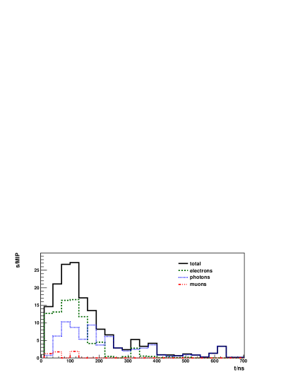
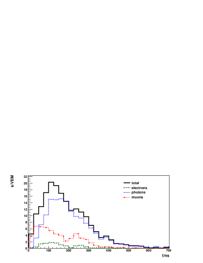
Figure 1: Comparison of WCD and scintillator traces. These two sets of traces correspond to a pair of scintillator station with no photon converter (left) and a WCD station (right). They are located at $413\text{\,}\mathrm{m}$ from the axis of a ${10}^{18}\text{\,}\mathrm{e}\mathrm{V}$ shower arriving at $38\text{\,}\mathrm{\SIUnitSymbolDegree}$. Note that, while the WCD station already has a significant contribution from muons, this is very small in the scintillator, which is dominated by the signal from electrons.

In order to study such a hybrid detector, we have implemented a simulation and reconstruction chain based on the Pierre Auger Observatory offline framework [10]. Using this chain, we have processed 20,000 simulated air showers produced with the CORSIKA [11] event generator. All these showers were generated using QGSJET II for high energy hadronic interaction simulations [12].

The parameter space chosen for the simulations has been determined by the energy and angular ranges under consideration. Additionally, it has been shown recently that real air-showers appear to have a larger muon component than simulated air-showers [13]. For this reason we have also performed the simulations with the number of muons artificially increased by a factor of two, which gives the observed muon contribution after an energy shift of about 28%. We have also investigated the effect of placing a certain amount of shielding on top of each scintillator station, as well as the effect of changing its area. In total there are 600 parameter combinations, with 100 simulated showers each, for a total of 60,000 simulated events. The parameters are shown in table 1.

Primaries	p, Fe
E (eV)	$e17.75\text{\,}$, ${10}^{18}\text{\,}$, $e18.25\text{\,}$
$\theta$	$0\text{\,}\mathrm{\SIUnitSymbolDegree}$, $25\text{\,}\mathrm{\SIUnitSymbolDegree}$, $38\text{\,}\mathrm{\SIUnitSymbolDegree}$, $48\text{\,}\mathrm{\SIUnitSymbolDegree}$, $60\text{\,}\mathrm{\SIUnitSymbolDegree}$
Area	$3\text{\,}\mathrm{m}^{2}$, $10\text{\,}\mathrm{m}^{2}$
$\mu_{scale}$	1, 2
Shield (rad. lengths)	0, 0.25, 0.5, 1, 2

Table 1: Parameters considered in the simulation of the response of the scintillator array.

The simulation of the interactions of the shower particles with the detector is done using the Geant4 package [14, 15]. The scintillation efficiencies used in the simulation correspond to the specifications for Bicron’s BD-416 scintillators: Polyvinyl Toluene scintillators with a nominal light yield of about ${10}^{4}\text{\,}\mathrm{p}\mathrm{h}\mathrm{o}\mathrm{t}\mathrm{o}\mathrm{n}\mathrm{s}\mathrm{/}\mathrm{M}\mathrm{e}\mathrm{V}$ and a density of $1.032\text{\,}\mathrm{g}\mathrm{/}\mathrm{c}\mathrm{m}^{3}$. The resulting scintillation photons are sampled at a frequency of $100\text{\,}\mathrm{M}\mathrm{H}\mathrm{z}$ to produce one FADC trace per station. The signal in each station is measured in units of Minimum Ionizing Particle equivalent, or MIP, where a MIP is given by the position of the peak of the Landau distribution for vertical muons. We then consider only stations with signals between 1 and $2000\text{\,}\mathrm{M}\mathrm{I}\mathrm{P}$ in order to simulate the dynamical range.

The arrival direction and core position of each event are currently estimated using only the WCDs. The arrival direction is determined by fitting a spherical shower front to the signal start times of the stations in the event. The core position is determined by adjusting a lateral distribution function (LDF) of the form

$$S_{\text{WCD}}(r)=S_{r_{0}}\,\left(\frac{r}{r_{0}}\right)^{-\beta}$$ (1)

to the total signal in the stations in the event. The $r_{0}$ parameter is $450\text{\,}\mathrm{m}$ and $S_{450}$ is the usual energy estimator for a WCD array with this grid spacing because it is the optimum distance for determining the signal [16]. The LDF for the scintillator array is described by the same formula and the optimum $r_{0}$ that will enhance the composition sensitivity still needs to be determined.

One typical event is displayed in figures 1 and 2. An example of the resulting average lateral distribution functions over 100 showers, for both the scintillator and the WCD array, can be seen in figure 3. Clearly, the slope of the proton and iron LDFs differ and there is a cross-over point where the signals are equal. This cross-over point depends on energy and zenith angle and this dependence is different for the two arrays. At ${10}^{18}\text{\,}\mathrm{e}\mathrm{V}$ and $0\text{\,}\mathrm{\SIUnitSymbolDegree}$, it is close to the shower axis for both arrays. As the zenith angle increases, the cross-over occurs at greater distances to the shower axis and for angles greater than $25\text{\,}\mathrm{\SIUnitSymbolDegree}$, which correspond to most of the aperture, it is located at more than 600 meters from the axis. At larger distances, the differences between proton and iron signals are similar in the scintillators and the WCDs since they both detect mostly muons in this radial range. Therefore, the largest difference in signal between proton and iron is found close to the axis.

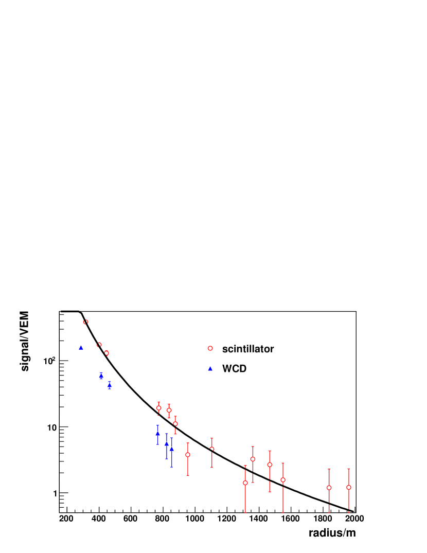
Figure 2: A typical ${10}^{18}\text{\,}\mathrm{e}\mathrm{V}$ shower arriving at $38\text{\,}\mathrm{\SIUnitSymbolDegree}$ showing the reconstructed LDF of the scintillator array.

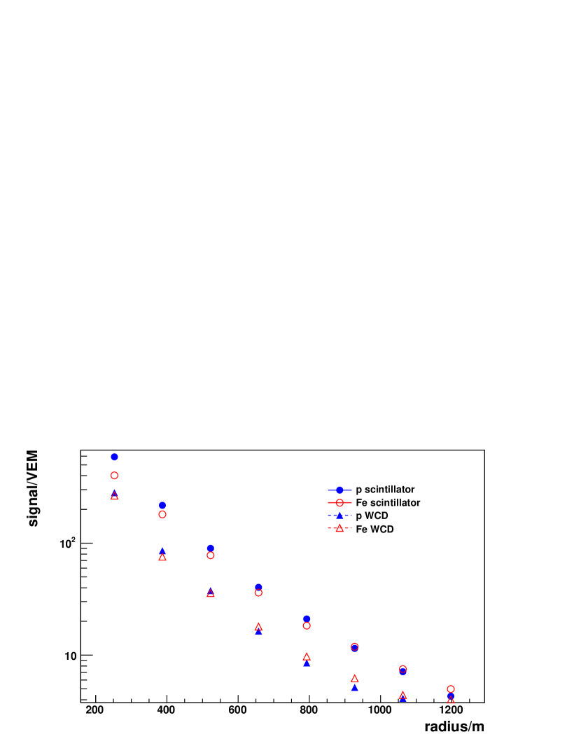
Figure 3: Comparison of the lateral distributions of $1\text{\times}{10}^{18}\text{\,}\mathrm{e}\mathrm{V}$ proton and iron induced air showers arriving at $38\text{\,}\mathrm{d}\mathrm{e}\mathrm{g}\mathrm{r}\mathrm{e}\mathrm{e}$ using a combined scintillator/WCD array. The area of each station is $10\text{\,}\mathrm{m}^{2}$. The muon component is artificially scaled by a factor of two.

For the reason mentioned above, we use the signal at 400 meters from the shower axis as the measure for the scintillator array signal. For each event we can then correlate the scintillator array signal ($S_{\text{sci}}$) with the WCD signal at 450 m ($S_{\text{WCD}}$). A typical contour plot of these quantities is shown in figure 4. One can model the dependence of the scintillator and WCD signals as a function of the energy and the mass number using

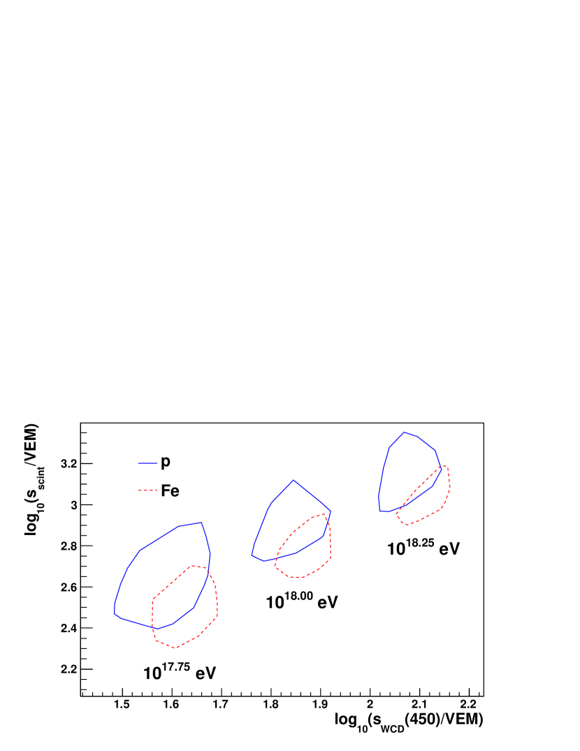
Figure 4: 68% contours of the $\log_{10}(S_{\text{sci}})-\log_{10}(S_{\text{WCD}})$ scatter plot. This corresponds to a zenith angle of $25\text{\,}\mathrm{\SIUnitSymbolDegree}$, $10\text{\,}\mathrm{m}^{2}$ stations with no lead photon converter and a scaling of the muon component by a factor of two.

$$\log_{10}S_{i}=a_{i}+b_{i}\log_{10}E+c_{i}\log_{10}A$$ (2)

This set of equations can then be inverted to find $\log_{10}E$ and $\log_{10}A$. The result is a mass estimator and an unbiased energy estimator.

There are various ways of measuring the discrimination power of a given statistic. One of them is the figure of merit:

$$f=\frac{\langle s_{Fe}\rangle-\langle s_{p}\rangle}{\sqrt{\sigma_{Fe}^{2}+\sigma_{p}^{2}}}.$$ (3)

The resulting average discrimination power, after correcting by the decrease in aperture with increasing zenith angle, is displayed in figure 5. We have used other multivariate methods as well as alternative measures of discrimination power, such as the efficiency at given purity levels. The results are qualitatively the same.

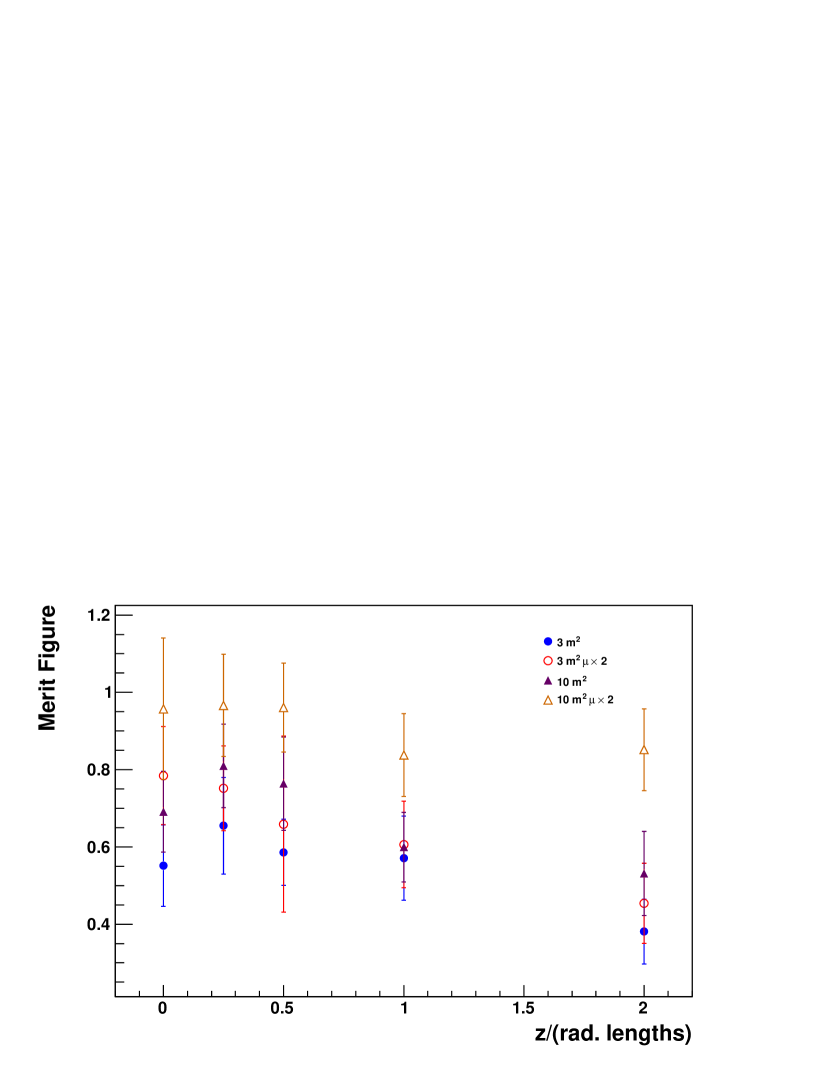
Figure 5: Average figure of merit as a function of the thickness of the lead shield. The different graphs correspond to the different detector areas and muon component scaling factor considered.

As an exercise to get an idea of the magnitude of the resulting uncertainties in the determination of the composition, one can pose the problem of determining the fraction of protons in a sample of proton and iron events.

Given a sample of equal number proton and iron showers, we can determine a cut value for the mass estimator such that the error rates of the first and second kind are equal ($\epsilon$). Let’s now consider a sample of N events where a fraction $f$ of them are protons. The observed number of proton-like ($s_{obs}$, the number of events passing the cut) and iron-like ($b_{obs}$) events depend on the number of actual signal and background events through the following equation:

$$\left(\begin{array}[]{c}s_{obs}\\ b_{obs}\end{array}\right)=\left(\begin{array}[]{cc}1-\epsilon&\epsilon\\ \epsilon&1-\epsilon\end{array}\right)\left(\begin{array}[]{c}fN\\ (1-f)N\end{array}\right)$$ (4)

and this equation can be inverted to estimate the proton fraction.

In order to judge the quality of the method, a common strategy is to split the sample into a training sample, from which we get the values of the coefficients in equations 2 and the value of the cut. We can also use a k-fold cross validation method. This consists in splitting the sample in sets of k events, taking half of the sets to form the training sample and use the rest as a test sample. This process is then repeated with different combinations of sets. The same procedure is repeated using the distributions of $X_{\text{max}}$ for proton and iron but in this case we limit the size of the test sample to 30% in order to take the combined effect of the aperture and limited duty cycle of a fluorescence detector into account. The result can be seen in figure 6.

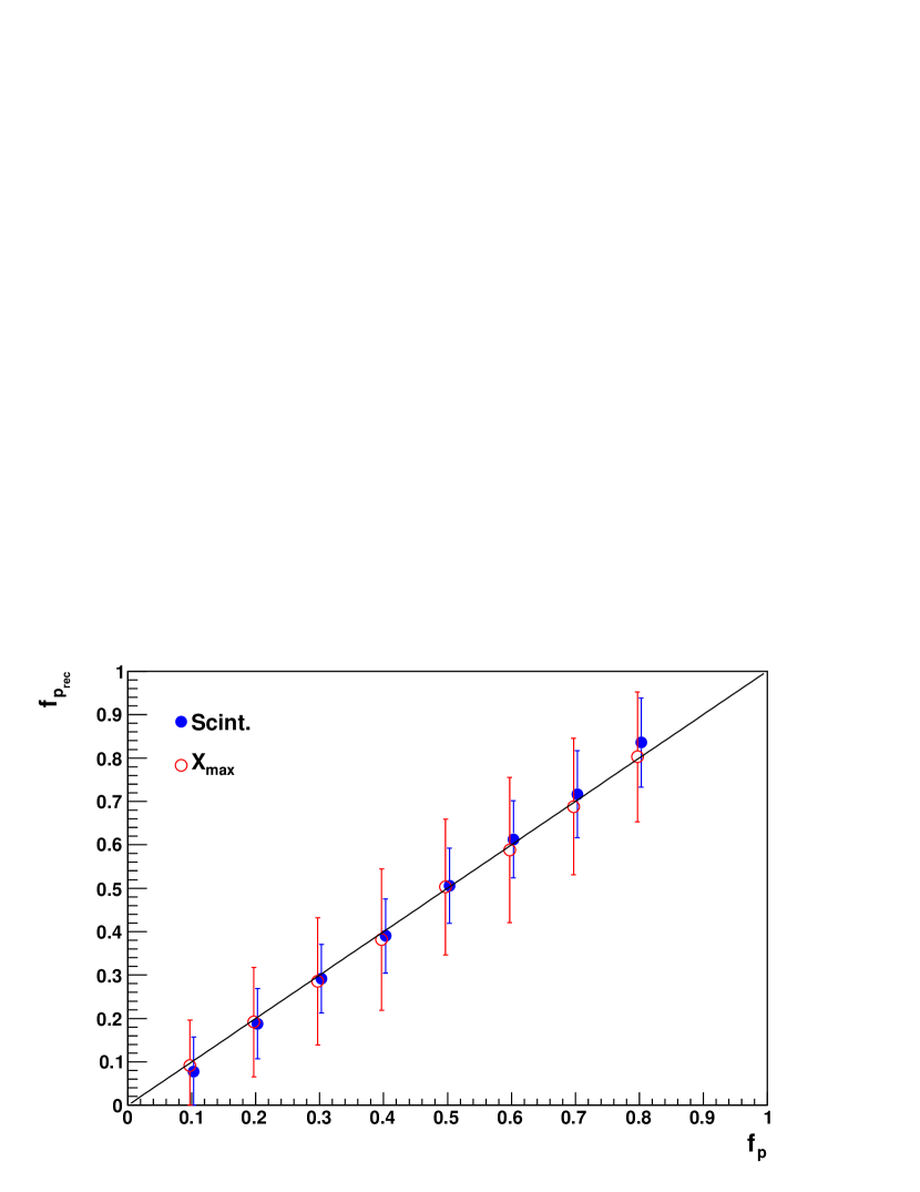
Figure 6: Cross validation of the proton fraction determination. This corresponds to ${10}^{18}\text{\,}\mathrm{e}$V showers arriving at $38\text{\,}\mathrm{\SIUnitSymbolDegree}$ and muon component scaled by a factor of two. The stations have an area of $3\text{\,}\mathrm{m}^{2}$ and 0.25 radiation length photon converters. The test sample for the $X_{\text{max}}$ technique is 30% of the sample for the combined array.

From this simple exercise we have learned that both methods give similar uncertainties in the determination of the proton fraction. In other words, that the combined scintillator/WCD array provides a composition estimate that is competitive with that from fluorescence detectors after one considers the fluorescence detectors’ limited duty-cycle. We are aware that the precise factor to penalize the $X_{\text{max}}$ measurement will depend on the relative apertures of the fluorescence detector and the surface detector and that there will be systematic errors deriving from the different strategies in training the classification and regression methods. This number will still give the right order of magnitude.

2 Summary

We have performed detailed simulations of the response of a combined scintillator/WCD array to air showers produced by cosmic ray with primary energies around $1\text{\times}{10}^{18}\text{\,}\mathrm{e}\mathrm{V}$. We have considered different configurations for the individual scintillator stations in order to optimize the composition sensitivity of the combined array.

We have found that an array of $10\text{\,}\mathrm{m}^{2}$ scintillator stations, together with the WCD array, can provide an estimate of the average mass composition that is competitive with $X_{\text{max}}$ measurements after differences in duty-cycle are considered and that the addition of photon converters on top of each station does not add to the separation power.

In this work we only considered a grid spacing of $750\text{\,}\mathrm{m}$ but we have noted that the highest separation between proton and iron occurs at small distances to the core. Better knowledge of the impact of smaller spacing and of the precise optimum distance at which to measure the scintillator signal requires further study.

References

- [1] W. D. Apel et al. [KASCADE Collaboration], Astropart. Phys. 31, 86 (2009)
- [2] T. Abu-Zayyad et al. [HiRes-MIA Collaboration], Astrophys. J. 557, 686 (2001)
- [3] R. U. Abbasi et al. [HiRes Collaboration], Phys. Rev. Lett. 104, 161101 (2010)
- [4] M. Unger, f. t. P. A. Collaboration, Nucl. Phys. Proc. Suppl. 190, 240-246 (2009).
- [5] M. Nagano, A. A. Watson, Rev. Mod. Phys. 72, 689-732 (2000).
- [6] H. Wahlberg [Pierre Auger Collaboration], Nucl. Phys. Proc. Suppl. 196 (2009) 195.
- [7] T. Antoni et al. [ KASCADE Collaboration ], Nucl. Instrum. Meth. A513, 490-510 (2003).
- [8] Manuel Platino et al. [Pierre Auger Collaboration] Proceedings of the 31st ICRC, 2009 [arXiv:0906.2354].
- [9] M. Kleifges et al. [Pierre Auger Collaboration] Proceedings of the 31st ICRC, 2009 [arXiv:0906.2354].
- [10] S. Argiro, S. L. C. Barroso, J. Gonzalez, L. Nellen, T. C. Paul, T. A. Porter, L. Prado, Jr., M. Roth et al., Nucl. Instrum. Meth. A580, 1485-1496 (2007).
- [11] D. Heck, G. Schatz, T. Thouw, J. Knapp and J. N. Capdevielle, FZKA-6019 (1998)
- [12] S. Ostapchenko, Phys. Rev. D83, 014018 (2011).
- [13] A. Castellina et al. [Pierre Auger Collaboration] Proceedings of the 31st ICRC, 2009 [arXiv:0906.2319]
- [14] S. Agostinelli et al. Nuclear Instruments and Methods in Physics Research A 506 (2003) 250–303
- [15] J. Allison et al. IEEE Transactions on Nuclear Science 53 No. 1 (2006) 270-278
- [16] D. Newton, J. Knapp, A. A. Watson, Astropart. Phys. 26, 414-419 (2007).