A note on a Marčenko-Pastur type theorem for time series

Abstract

In this note we develop an extension of the Marčenko-Pastur theorem to time series model with temporal correlations. The limiting spectral distribution (LSD) of the sample covariance matrix is characterised by an explicit equation for its Stieltjes transform depending on the spectral density of the time series. A numerical algorithm is then given to compute the density functions of these LSD’s.

T1The research of the author was supported partly by a HKU Start-up grant.

1 Introduction

Let $\{\mathbf{X}_{j}\},j=1,\ldots,n$ be a sequence of $p$-dimensional real-valued random vectors and consider the associated empirical covariance matrix

$$S_{n}=\frac{1}{n}\sum_{j=1}^{n}\mathbf{X}_{j}\mathbf{X}_{j}^{\top}.$$ (1)

The study of the empirical spectral distribution (ESD) $F_{n}$ of $S_{n}$, i.e. the distribution generated by its (real-valued) eigenvalues, goes back to Wishart in 1920’s. A milestone work by Marčenko and Pastur (1967) states that if both sample size $n$ and data dimension $p$ proportionally grow to infinity such that $\lim p/n=c$ for some positive $c>0$ and all the coordinates of all the vectors $\mathbf{X}_{j}$’s are i.i.d. with mean zero and variance 1, then $F_{n}$ converges to a nonrandom distribution. This limiting spectral distribution (LSD), named after them as the Marčenko-Pastur distribution of index $c$ has a density function

$$f(x)=\frac{1}{2\pi cx}\sqrt{(b-x)(x-a)},\quad a\leq x\leq b,$$ (2)

with $a=(1-\sqrt{c})^{2}$ and $b=(1+\sqrt{c})^{2}$ defining the support interval and has a point mass $1-1/c$ at the origin if $c>1$. Further refinements are made successively by many researchers including Jonsson (1982), Wachter (1978) and Yin (1986).

An important work by Silverstein (1995) aimed at relaxing the independence structure between the coordinates of the $\mathbf{X}_{j}$’s and considered random vectors of form $\mathbf{Y}_{j}=T_{p}^{1/2}\mathbf{X}_{j}$ where $(T_{p})$ is a sequence of non-negative definite matrices. Assuming that $(T_{p})$ is bounded in spectral norm and the sequence of ESD of $(T_{p})$ has a weak limit $H$, he established a (strong) LSD for the sample covariance matrix $n^{-1}\sum Y_{j}Y_{j}^{\top}$ and provides a characteristic equation for its Stieltjes transform. Despite a big step made by this generalisation, it still does not cover all possible correlation patterns of coordinates. Pursuing these efforts, a recent work by Bai and Zhou (2008) pushes a step further Silverstein’s result by allowing a very general pattern for correlations between the coordinates of the $\mathbf{X}_{j}$’s satisfying a mild moment conditions.

In this work, we extend such Marčenko-Pastur type theorems along another direction by considering time series observations instead of an i.i.d. sample. Let us first consider an univariate real-valued linear process

$$z_{t}=\sum_{k=0}^{\infty}\phi_{k}\varepsilon_{t-k},\quad t\in\mathbb{Z},$$ (3)

where $(\varepsilon_{k})$ is a real-valued and weakly stationary white noise with mean zero and variance 1. The $p$-dimensional process $(\mathbf{X}_{t})$ considered in this paper will be made by $p$ independent copies of the linear process $(z_{t})$, i.e. for $\mathbf{X}_{t}=(X_{1t},\ldots,X_{pt})^{\top}$,

$$X_{it}=\sum_{k=0}^{\infty}\phi_{k}\varepsilon_{i,t-k},\quad t\in\mathbb{Z},$$ (4)

where the $p$ coordinate processes $\{(\varepsilon_{1,t},\ldots,\varepsilon_{p,t})\}$ are independent copies of the univariate error process $\{\varepsilon_{t}\}$ in (3). Let $\mathbf{X}_{1},\ldots,\mathbf{X}_{n}$ be the observations of the time series at time epochs $t=1,\ldots,n$. Again we are interested in the ESD of the sample covariance matrix $S_{n}$ in (1).

The author should mention that a similar problem has been considered in Jin et al. (2009). However we propose much more general results in this note since firstly their results are limited to ARMA-type processes instead of a general linear process considered here and secondly, they do not find a general equation as the one proposed in Theorem 1 below except for two simplest particular cases of AR(1) and MA(1).

2 A Marčenko-Pastur type theorem for linear processes

Recall that the Stieltjes transform $s_{\mu}$ of a probability measure $\mu$ on the real line is a map from the set $\mathbb{C}^{+}$ of complex numbers with positive imaginary part onto itself and defined by

$$s_{\mu}(z)=\int\frac{1}{x-z}\mu(dx),\quad z\in\mathbb{C}^{+}.$$

We always employ an usual convention that for any complex number $z$, $\sqrt{z}$ denotes its square root with nonnegative imaginary part.

Theorem 1.

Assume that the following conditions hold:

1. The dimensions $p\to\infty$, $n\to\infty$ and $p/n\to c\in(0,\infty)$;

2. The error process has a fourth moment: $\mathbb{E}\varepsilon_{t}^{4}<\infty$;

3. The linear filter $(\phi_{k})$ is absolutely summable, i.e. $\displaystyle\sum\limits_{k=0}^{\infty}|\phi_{k}|<\infty$.

Then almost surely the ESD of $S_{n}$ tends to a non-random probability distribution $F$. Moreover, the Stieltjes transform $s=s(z)$ of $F$ (as a mapping from $\mathbb{C}^{+}$ into $\mathbb{C}^{+}$) satisfies the equation

$$z=-\frac{1}{s}+\frac{1}{2\pi}\int_{0}^{2\pi}\frac{1}{cs+\{2\pi f(\lambda)\}^{-1}}\,d\lambda\leavevmode\nobreak\ ,$$ (5)

where $f(\lambda)$ is the spectral density of the linear process $(z_{t})$:

$$f(\lambda)=\frac{1}{2\pi}\left|\sum_{k=0}^{\infty}\phi_{k}e^{ik\lambda}\right|^{2},\quad\lambda\in[0,{2\pi}).$$ (6)

The proof of the theorem is postponed to Section 4. Let us mention that although the case $c=0$ is beyond the scope of Theorem 1, Equation (5) leads in this case to the solution $s(z)=1/(\gamma_{0}-z)$, that is the LSD would be the Dirac mass at $\gamma_{0}={\mbox{ Var}}(X_{it})$. This conjectures an extension of Theorem 1 to the so-called “very large $p$ and small $n$” asymptotics where one assumes $p\rightarrow\infty$, $n\rightarrow\infty$ and $p/n\rightarrow 0$. Indeed, in this scenario taking into account that the population covariance matrix of $\mathbf{X}_{t}$ equals $\gamma_{0}I_{p}$, one can expect that the sample eigenvalues of $S_{n}$ stay close to the population ones (all equal to $\gamma_{0}$). Note that such results exist for i.i.d. sequence $(\mathbf{X}_{t})$ with i.i.d. components (see Bai and Yin, 1988).

2.1 Support of the LSD $F$

Starting from Eq. 5 and following the techniques devised in Silverstein and Choi (1995), we can describe precisely the support of the LSD $F$ in previous theorem.

Let $a$ and $b$ be respectively the minimum and the maximum of the function $2\pi f$ over $[0,2\pi]$. As $f$ is infinitely differentiable and positive everywhere, both $a$ and $b$ are attained and the range of $2\pi f$ is exactly the interval $[a,b]$. We will always exclude the situation $a=0$ since it corresponds to a special class of linear processes, namely non-invertible ARMA processes, see Grenander and Szegö (1958, chap. 9), which has no practical interest for applications. Therefore the map $s\mapsto z=g(s)$ in Eq.(5) has a trace for real-valued $s$ providing $s\notin[-\frac{1}{ac},-\frac{1}{bc}]$. Figure 1 depicts this map for both $c<1$ and $c>1$ cases.

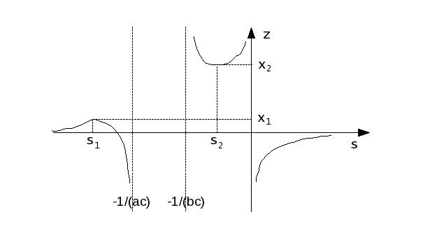
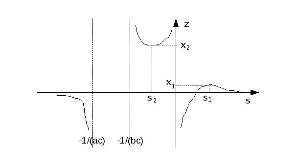
Figure 1: Determination of the support $[x_{1},x_{2}]$ of the LSD. Left panel $c>1$ and right panel $c<1$.

The following proposition is a straightforward application of results from Silverstein and Choi (1995) and we then omit its proof.

Proposition 1.

With the map $g:\leavevmode\nobreak\ s\mapsto z=g(s)$ in Eq.(5) restricted to real $s\notin[-\frac{1}{ac},-\frac{1}{bc}]$ (Figure 1) the following holds:

1. The LSD $F$ has a compact support $[x_{1},x_{2}]\subset[0,\infty)$ on which it has a continuous density function. In case of $c>1$, $F$ has an additional point mass $1-1/c$ at the origin.

2. When $c>1$, the map $g$ has an unique maximum $s_{1}$ on $(-\infty,-\frac{1}{ac})$ and an unique minimum $s_{2}$ on $(-\frac{1}{bc},0)$ and we have The edges of the support interval are given by these local extrema: $x_{1}=g(s_{1})$ and $x_{2}=g(s_{2})$.

3. When $c<1$, the map $g$ has an unique maximum $s_{1}$ on $(0,\infty)$ and an unique minimum $s_{2}$ on $(-\frac{1}{bc},0)$. The edges of the support interval (for the absolutely continuous component) are again given by these local extrema: $x_{1}=g(s_{1})$ and $x_{2}=g(s_{2})$.

2.2 Application to an ARMA process

For simplicity, we consider the simplest causal ARMA(1,1) process for the coordinates:

$$z_{t}=\phi z_{t-1}+\varepsilon_{t}+\theta\varepsilon_{t-1},\quad t\in\mathbb{Z},$$

where $|\phi|<1$ and $\theta$ is real. The aim is to find a simplified form of general equation (5). We have

$$\frac{1}{2\pi f(\lambda)}=\left|\frac{1-\phi e^{i\lambda}}{1+\theta e^{i\lambda}}\right|^{2}\leavevmode\nobreak\ ,$$

and

$$I = \frac{1}{2\pi}\int_{0}^{2\pi}\frac{1}{cs+\{2\pi f(\lambda)\}^{-1}}\,d\lambda=\frac{1}{2\pi i}\oint_{|\xi|=1}\frac{1}{cs+\left|\frac{1-\phi\xi}{1+\theta\xi}\right|^{2}}\frac{d\xi}{\xi}.$$

By a lengthy but elementary calculation of residues detailed in Section 4, we find

$$I=\frac{\theta}{cs\theta-\phi}\left\{1-\frac{(\phi+\theta)(1+\phi\theta)}{\theta(cs\theta-\phi)}\frac{\epsilon(\alpha)}{\sqrt{\alpha^{2}-4}}\right\},$$ (7)

with

$$\alpha=\frac{cs(1+\theta^{2})+1+\phi^{2}}{cs\theta-\phi},\qquad\epsilon(\alpha)=\mathop{\hbox{\rm sgn}}(\Im\alpha)\leavevmode\nobreak\ .$$ (8)

Therefore for an ARMA(1,1) process, the general equation (5) reduces to

$$z=-\frac{1}{s}+\frac{\theta}{cs\theta-\phi}-\frac{(\phi+\theta)(1+\phi\theta)}{(cs\theta-\phi)^{2}}\frac{\epsilon(\alpha)}{\sqrt{\alpha^{2}-4}}\leavevmode\nobreak\ .$$ (9)

Let us mention that it is important to have an explicit formula for the integral in (5) to implement numerical algorithms like the one proposed in Section 3 in order to compute the density function of the LSD $F$.

Case of an AR(1). For this particular case, we have $\theta=0$ and $\alpha=-(cs+1+\phi^{2})/\phi$. As $\Im s>0$, $\epsilon(\alpha)=\mathop{\hbox{\rm sgn}}(-\phi)$. It follows that

$$-\frac{(\phi+\theta)(1+\phi\theta)}{(cs\theta-\phi)^{2}}\frac{\epsilon(\alpha)}{\sqrt{\alpha^{2}-4}}=\frac{\mathop{\hbox{\rm sgn}}(-\phi)}{-\phi}\frac{1}{\sqrt{\frac{(cs+1+\phi^{2})^{2}}{\phi^{2}}-4}}$$

$$\quad=\frac{1}{|\phi|}\frac{1}{\sqrt{\frac{(cs+1+\phi^{2})^{2}}{\phi^{2}}-4}}=\frac{1}{\sqrt{(cs+1+\phi^{2})^{2}-4\phi^{2}}}\leavevmode\nobreak\ .$$

Therefore the Stieltjes transform $s$ of the LSD is solution to a simpler equation

$$z=-\frac{1}{s}+\frac{1}{\sqrt{(cs+1+\phi^{2})^{2}-4\phi^{2}}}\leavevmode\nobreak\ .$$ (10)

It is worth noticing that if we further assume $\phi=0$, this equation reduces to $z=-1/s+1/(cs+1)$ which characterises the standard Marčenko-Pastur law with i.i.d. coordinates. Furthermore, for the determination of the support $[x_{1},x_{2}]$ of the LSD, we notice that

$$2\pi f(\lambda)=\frac{1}{|1-\phi e^{i\lambda}|^{2}},$$

so that its extrema are $a=1/(1+|\phi|)^{2}$ and $b=1/(1-|\phi|)^{2}$ (see Figure 1).

Case of an MA(1). Here we have $\phi=0$ and

$$\alpha=\frac{1}{\theta}\left(\frac{1}{cs}+1+\theta^{2}\right)\leavevmode\nobreak\ .$$

Hence $\epsilon(\alpha)=-\mathop{\hbox{\rm sgn}}(\theta)$ and it is readily checked out that the Stieltjes transform of the LSD is solution to the equation

$$z=-\frac{1}{s}+\frac{1}{cs}+\frac{1}{c^{2}s^{2}}\frac{1}{\sqrt{\left(\frac{1}{cs}+1+\theta^{2}\right)^{2}-4\theta^{2}}}\leavevmode\nobreak\ .$$ (11)

Again if we further assume $\theta=0$, this equation reduces to the one for the standard Marčenko-Pastur law. Furthermore, for the determination of the support $[x_{1},x_{2}]$ of the LSD, we notice that

$$2\pi f(\lambda)={|1+\theta e^{i\lambda}|^{2}},$$

so that its extrema are $a=(1-|\theta|)^{2}$ and $b=(1+|\theta|)^{2}$ (see Figure 1).

3 A numerical method for computing the LSD density function

In this section we provide a numerical algorithm for the computation of the density function $h$ of the LSD defined in Eq.(5) through its Stieltjes transform $s$. We have

$$s=\frac{1}{-z+A(s(z))}$$

with

$$A(s(z))=\frac{1}{2\pi}\int_{0}^{2\pi}\frac{1}{cs+\{2\pi f(\lambda)\}^{-1}}\,d\lambda\leavevmode\nobreak\ .$$

The algorithm we propose is of fixed-point type.

Algorithm

For a given real $x$, let $\varepsilon$ be small enough positive value and set $z=x+i\varepsilon.$

Choose an initial value $s_{0}(z)=u+i\varepsilon$ and iterate for $k\geq 0$ the above mapping

$$s_{k+1}(z)=\{-z+A(s_{k}(z))\}^{-1}\leavevmode\nobreak\ ,$$

until convergence and let $s_{K}(z)$ be the final value.

Define the estimate of the density function $h(x)$ to be

$$\widehat{h}(x)=\frac{1}{\pi}\Im s_{K}(z)\leavevmode\nobreak\ .\hskip 56.9055pt\blacksquare$$

It is well-known that this iterated map has good contraction properties guaranteeing the convergence of the algorithm. There are however two issues which need a careful consideration. First the integral operator $A$ is usually approximated by a numeric routine and because of a high number of calls to $A$, the resulting algorithm is slow. In this aspect analytic formula for $A$ when available are well acknowledged as Eq.(9) in the case of an ARMA(1,1).

A second issue is that overall we first need to determine the support interval $[x_{1},x_{2}]$ of the density function $h$. This is handled with the help of description of $x_{j}$’s given in Proposition 1.

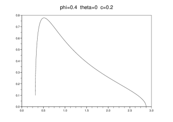
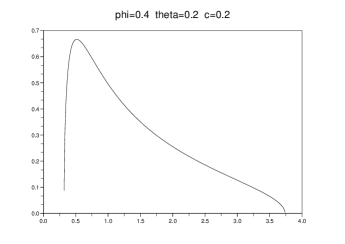
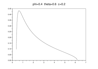
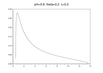
Figure 2: Densities of the LSD from ARMA(1,1) model. Left to right and top to bottom: $(\phi,\theta,c)=$ (0.4, 0, 0.2), (0.4, 0.2, 0.2), (0.4, 0.6, 0.2), and (0.8, 0.2, 0.2).

For four ARMA(1,1) models listed in Table 1, we have used this algorithm with the map $A$ defined in (9) to get the density plots displayed in Figure 2.

Table 1: ARMA(1,1) models for density plots. Reference support interval for Marčenko-Pastur law of index $c=0.2$ is $[0.306,2.094]$.

Parameters $(\phi,\theta,c)$	Estimated support $[x_{1},x_{2}]$
(0.4, 0, 0.2)	[0.310, 2.875]
(0.4, 0.2, 0.2)	[0.319, 3.737]
(0.4, 0.6, 0.2)	[0.382, 6.186]
(0.8, 0.2, 0.2)	[0.485, 13.66]

Compared to the reference standard Marčenko-Pastur law with the same dimension to sample ratio $c$, the above density functions from ARMA models share a similar shape with however a support interval getting larger and larger with increasing ARMA coefficients $\phi$ and $\theta$.

4 Proofs

Proof of Theorem 1

Recall that the $p$ coordinates of the vectors $\mathbf{X}_{1},\ldots,\mathbf{X}_{n}$ are i.i.d. while the temporal covariances ${\mbox{ Cov}}(X_{is},X_{it})$ are by definition those of $(z_{t})$: for all $1\leq i\leq p$,

$${\mbox{ Cov}}(X_{is},X_{it})={\mbox{ Cov}}(z_{s},z_{t})=\gamma_{t-s},\quad 1\leq s,t\leq n\leavevmode\nobreak\ .$$

Let $\widetilde{f}=2\pi f$. It follows that the covariance matrix $T_{n}$ of each coordinate process $(X_{i1},\ldots,X_{in})$ equals to the $n$-th order Toeplitz matrix associated to $\widetilde{f}$:

$$T_{n}(s,t)=\gamma_{t-s},\quad\quad 1\leq s,t\leq n\leavevmode\nobreak\ ,$$

and

$$\widetilde{f}(\lambda)=\sum_{k=-\infty}^{\infty}\gamma_{k}e^{ik\lambda}\leavevmode\nobreak\ ,\quad\lambda\in[0,{2\pi}).$$

We are going to apply Theorem 1.1 of Bai and Zhou (2008) for a strong limit of the ESD of the sample covariance matrix $S_{n}=\frac{1}{n}\sum\limits_{t=1}^{n}\mathbf{X}_{t}\mathbf{X}_{t}^{\top}$. Under the assumptions made, all the conditions of this theorem are satisfied except that we need to ensure a weak limit for spectral distributions of $(T_{n})$.

The function $\widetilde{f}$ belongs to the Wiener class, i.e. the sequence of its Fourier coefficients is absolutely summable. Moreover note that $\widetilde{f}$ is infinitely differentiable, its minimum $a$ and maximum $b$ are attained. According to the fundamental eigenvalue distribution theorem of Szegö for Toeplitz forms, see Grenander and Szegö (1958, sect. 5.2), for any function $\varphi$ continuous on $[a,b]$ and denoting the eigenvalues of $T_{n}$ by $\sigma_{1}^{(n)},\ldots,\sigma_{n}^{(n)}$, it holds that

$$\lim_{n\to\infty}\frac{1}{n}\sum_{k=1}^{n}\varphi(\sigma_{k}^{(n)})=\frac{1}{2\pi}\int_{0}^{{2\pi}}\varphi(\widetilde{f}(\lambda))d\lambda\leavevmode\nobreak\ .$$

Consequently, the ESD of $T_{n}$ (i.e. distribution generated by the $\sigma_{n}^{(k)}$’s) weakly converges to a nonrandom distribution $H$ with support $[a,b]$ and defined by

$$H(x)=\frac{1}{2\pi}\int_{0}^{{2\pi}}\mbox{\large 1}_{\{\widetilde{f}(\lambda)\leq x\}}d\lambda\leavevmode\nobreak\ ,$$ (12)

and we have for $\varphi$ as above,

$$\int_{0}^{\infty}\varphi(x)dH(x)=\frac{1}{2\pi}\int_{0}^{{2\pi}}\varphi(\widetilde{f}(\lambda))d\lambda\leavevmode\nobreak\ .$$ (13)

Furthermore, by application of Theorem 1.1 of Bai and Zhou (2008), it holds that the ESD of $\frac{n}{p}S_{n}$ converges almost surely to a nonrandom probability distribution whose Stieltjes transform $m$ solves the equation

$$z = -\frac{1}{m}+\frac{1}{c}\int\frac{x}{1+mx}dH(x)$$

$$= -\frac{1}{m}+\frac{1}{2\pi c}\int_{0}^{2\pi}\frac{1}{m+1/{\widetilde{f}}}d\lambda\leavevmode\nobreak\ ,$$

where we have used (13) in the last equation. The equation(5) follows by observing the relation $s(z)=\frac{1}{c}m(z/c)$.

Proof of Equation (7)

The aim is to evaluate the integral

$$I=\frac{1}{2\pi i}\oint_{|\xi|=1}\frac{1}{cs+\left|\frac{1-\phi\xi}{1+\theta\xi}\right|^{2}}\frac{d\xi}{\xi}.$$

Let $m=cs$ in this computation of residues. We have

$$I = \frac{1}{2\pi i}\oint_{|\xi|=1}\frac{1+\theta^{2}+\theta(\xi+\xi^{-1})}{m\left\{1+\theta^{2}+\theta(\xi+\xi^{-1})\right\}+\left\{1+\phi^{2}-\phi(\xi+\xi^{-1})\right\}}\frac{d\xi}{\xi}$$

$$= \frac{\theta}{m\theta-\phi}\frac{1}{2\pi i}\oint_{|\xi|=1}\left\{\frac{1}{\xi}-\frac{(\phi+\theta)(1+\phi\theta)}{\theta(m\theta-\phi)}\frac{1}{\xi^{2}+1+\alpha\xi}\right\}d\xi\leavevmode\nobreak\$$

$$= \frac{\theta}{m\theta-\phi}\left\{1-\frac{(\phi+\theta)(1+\phi\theta)}{\theta(m\theta-\phi)}\frac{1}{2\pi i}\oint_{|\xi|=1}\frac{d\xi}{P(\xi)}\right\},$$

with

$$P(\xi)=\xi^{2}+\alpha\xi+1,\quad\alpha=\frac{m(1+\theta^{2})+1+\phi^{2}}{m\theta-\phi}.$$

Let $\xi_{1},\xi_{2}$ be the roots of $P(\xi)=\xi^{2}+1+\alpha\xi$. Then

$$\frac{1}{P(\xi)}=\left(\frac{1}{\xi-\xi_{1}}-\frac{1}{\xi-\xi_{2}}\right)\frac{1}{\xi_{1}-\xi_{2}}\leavevmode\nobreak\ .$$

As $\xi_{1}\xi_{2}=1$, only one of the two poles is inside the unit circle. It is readily checked that if $\Im\alpha>0$, then $|\xi_{1}|<|\xi_{2}|$ and

$$\frac{1}{2\pi i}\oint_{|\xi|=1}\frac{d\xi}{P(\xi)}=\frac{1}{\xi_{1}-\xi_{2}}=\frac{1}{\sqrt{\alpha^{2}-4}}.$$

Otherwise we have $|\xi_{1}|>|\xi_{2}|$ and the integral has an opposite sign. Summarising both cases we get

$$\frac{1}{2\pi i}\oint_{|\xi|=1}\frac{d\xi}{P(\xi)}=\frac{\epsilon(\alpha)}{\sqrt{\alpha^{2}-4}},$$

with $\epsilon(\alpha)=\mathop{\hbox{\rm sgn}}(\Im(\alpha))$. Equation (7) is proved.

Acknowledgement.  The author is grateful to Jack Silverstein for several insightful discussions on the problem studied here, particularly for pointing to me the numerical method of Section 3. We also thank a referee for important comments on the paper.

References

- Bai and Zhou (2008) Bai, Z., Zhou, W., 2008. Large sample covariance matrices without independence structures in columns. Statist. Sinica 18 (2), 425–442.
- Bai and Yin (1988) Bai, Z. D., Yin, Y. Q., 1988. A convergence to the semicircle law. Ann. Probab. 16 (2), 863–875.
- Grenander and Szegö (1958) Grenander, U., Szegö, G., 1958. Toeplitz forms and their applications. California Monographs in Mathematical Sciences. University of California Press, Berkeley.
- Jin et al. (2009) Jin, B., Wang, C., Miao, B., Lo Huang, M., 2009. Limiting spectral distribution of large-dimensional sample covariance matrices generated by varma. J. Multivariate Anal. 100, 2112–2125.
- Jonsson (1982) Jonsson, D., 1982. Some limit theorems for the eigenvalues of a sample covariance matrix. J. Multivariate Anal. 12 (1), 1–38.
- Marčenko and Pastur (1967) Marčenko, V., Pastur, L., 1967. Distribution of eigenvalues for some sets of random matrices. Math. USSR-Sb 1, 457–483.
- Silverstein (1995) Silverstein, J. W., 1995. Strong convergence of the empirical distribution of eigenvalues of large-dimensional random matrices. J. Multivariate Anal. 55 (2), 331–339.
- Silverstein and Choi (1995) Silverstein, J. W., Choi, S.-I., 1995. Analysis of the limiting spectral distribution of large-dimensional random matrices. J. Multivariate Anal. 54 (2), 295–309.
- Wachter (1978) Wachter, K. W., 1978. The strong limits of random matrix spectra for sample matrices of independent elements. Ann. Probability 6 (1), 1–18.
- Yin (1986) Yin, Y. Q., 1986. Limiting spectral distribution for a class of random matrices. J. Multivariate Anal. 20 (1), 50–68.