Discovery and Atmospheric Characterization of Giant Planet Kepler-12b:
An Inflated Radius Outlier

Abstract

We report the discovery of planet Kepler-12b (KOI-20), which at $1.695\pm 0.030$ $R_{\mathrm{J}}$ is among the handful of planets with super-inflated radii above 1.65 $R_{\mathrm{J}}$. Orbiting its slightly evolved G0 host with a 4.438-day period, this $0.431\pm 0.041$ $M_{\mathrm{J}}$ planet is the least-irradiated within this largest-planet-radius group, which has important implications for planetary physics. The planet’s inflated radius and low mass lead to a very low density of $0.111\pm 0.010$ g cm^-3. We detect the occultation of the planet at a significance of 3.7$\sigma$ in the Kepler bandpass. This yields a geometric albedo of $0.14\pm 0.04$; the planetary flux is due to a combination of scattered light and emitted thermal flux. We use multiple observations with Warm Spitzer to detect the occultation at 7$\sigma$ and 4$\sigma$ in the 3.6 and 4.5 $\mu$m bandpasses, respectively. The occultation photometry timing is consistent with a circular orbit, at $e<0.01$ (1$\sigma$), and $e<0.09$ (3$\sigma$). The occultation detections across the three bands favor an atmospheric model with no dayside temperature inversion. The Kepler occultation detection provides significant leverage, but conclusions regarding temperature structure are preliminary, given our ignorance of opacity sources at optical wavelengths in hot Jupiter atmospheres. If Kepler-12b and HD 209458b, which intercept similar incident stellar fluxes, have the same heavy element masses, the interior energy source needed to explain the large radius of Kepler-12b is three times larger than that of HD 209458b. This may suggest that more than one radius-inflation mechanism is at work for Kepler-12b, or that it is less heavy-element rich than other transiting planets.

1. Introduction

Transiting planets represent an opportunity to understand the physics of diverse classes of planets, including mass-radius regimes not found in the solar system. The knowledge of the mass and radius of an object immediately yields the bulk density, which can be compared to models to yield insight into the planet’s internal composition, temperature, and structure (e.g., Miller & Fortney, 2011). Subsequent observations, at the time of the planet’s occultation (secondary eclipse) allow for the detection of light emitted or scattered by the planet’s atmosphere, which can give clues to a planet’s dayside temperature structure and chemistry (Marley et al., 2007; Seager & Deming, 2010). NASA’s Kepler Mission was launched on 7 March 2009 with the goal of finding Earth-sized planets in Earth-like orbits around Sun-like stars (Borucki et al., 2010). While working towards this multi-year goal, it is also finding an interesting menagerie of larger and hotter planets that are aiding our understanding of planetary physics.

Early on in the mission, followup radial velocity resources preferentially went to giant planets, for which it would be relatively easy to confirm their planetary nature through a measurement of planetary mass. This is how the confirmation of planet Kepler-12b was made, at first glance a relatively standard “hot Jupiter” in a 4.438 day orbit. However, upon further inspection, the mass and radius of Kepler-12b make it an interesting planet from the standpoint of the now-familiar “radius anomaly” of transiting giant planets (e.g. Charbonneau et al., 2007; Burrows et al., 2007; Laughlin et al., 2011). Given our current understanding of strongly-irradiated giant planet thermal evolution, around 1/3 to 1/2 of known transiting planets are larger than models predict for several-Gyr-old planets that cool and contract under intense stellar irradiation (Miller et al., 2009).

The observation that many Jupiter- and Saturn-mass planets are be larger than 1.0 Jupiter-radii can be readily understood. It is the magnitude of the effect that still needs explanation. The first models of strongly irradiated planets yielded the prediction that these close-in planets would be inflated in radius compared to Jupiter and Saturn (Guillot et al., 1996). The high incident flux drives the radiative convective boundary from less than a bar, as in Jupiter, to pressures near a kilobar. The thick radiative zone transports less flux than a fully convective atmosphere, thereby slowing interior cooling, which slows contraction. A fairly uniform prediction of these strongly irradiated models is that $1.2-1.3$ $R_{\mathrm{J}}$ is about the largest radii predicted for planets several gigayears-old (Bodenheimer et al., 2003; Burrows et al., 2007; Fortney et al., 2007; Baraffe et al., 2008). However, planets commonly exceed this value.

The mechanism that leads to the radius anomaly has not yet been definitively identified. However, constraints are emerging. One is planet radius vs. incident flux, which could also be thought of as radius vs. equilibrium temperature, with an assumption regarding planetary Bond albedos. Figure 1 shows planet radii vs. incident flux for the transiting systems with confirmed masses. Since low-mass planets are relatively easier to inflate to large radii than higher mass planets (e.g. Miller et al., 2009), we plot the planets in three mass bins. The lowest mass bin is Saturn-like masses, while the middle mass bin is Jupiter-like masses. The upper mass bin ends at 13 $M_{\mathrm{J}}$, the deuterium burning limit. Kepler-12b is shown as a black filled circle. The largest radius planets are generally the most highly irradiated (Kovács et al., 2010; Laughlin et al., 2011; Batygin et al., 2011). The near-universality of the inflation, especially at high incident fluxes, now clearly argues for a mechanism that affects all close-in planets (Fortney et al., 2006), rather than one that affects only some planets. The distribution of the radii could then be understood in terms of differing magnitudes of the inflation mechanism, together with different abundances of heavy elements within the planets (Fortney et al., 2006; Guillot et al., 2006; Burrows et al., 2007; Miller & Fortney, 2011; Batygin et al., 2011).

Within this emerging picture, outlier points are particularly interesting: those that are especially large, given their incident flux. These are the super-inflated planets with radii of 1.7 $R_{\mathrm{J}}$ or larger. These include WASP-12b (Hebb et al., 2009), TrES-4b (Mandushev et al., 2007; Sozzetti et al., 2009), WASP-17b (Anderson et al., 2010), and now Kepler-12b, which is the least irradiated of the four. In the following we describe the discovery of Kepler-12b, along with the initial characterization of the planet’s atmosphere.

Transiting planets enable the characterization of exoplanet atmospheres. The Spitzer Space Telescope has been especially useful for probing the dayside temperature structure of close-in planetary atmospheres, as thermal emission from the planets can readily be detected by Spitzer at wavelengths longer than 3 $\mu$m. Data sets are becoming large enough that one can begin to search for correlations in the current detections (Knutson et al., 2010; Cowan & Agol, 2011).

A powerful new constraint of the past two years is the possibility of joint constraints in the infrared, from Spitzer, and the optical, from space telescopes like CoRoT (e.g., Gillon et al., 2010; Deming et al., 2011) and Kepler (Désert et al., 2011a). The leverage from optical wavelengths comes from a measurement (or upper limit) of the geometric albedo of the planet’s atmosphere, although this is complicated by a mix of thermal emission and scattered light both contributing for these planets. Detection of relatively low geometric albedos $A_{\mathrm{g}}<0.15$ is consistent with cloud-free models of hot Jupiter atmospheres (Sudarsky et al., 2003; Burrows et al., 2008), and can inform our understanding of what causes the temperature inversions in many hot Jupiter atmospheres (Spiegel & Burrows, 2010).

In this paper we discuss all aspects of the detection, validation, confirmation, and characterization of the planet. Section 2 discusses the detection of the planet by Kepler, while §3 covers false-positive rejection and radial velocity confirmation. Section 4 gives the global fit to all data sets to derive stellar and planetary parameters, while §5 concerns the observational and modeling aspects of atmospheric characterization. Section 6 is a discussion of the planet’s inflated radius amongst its peers, while §7 gives our conclusions.

2. Discovery

The Kepler science data for the primary transit search mission are the long cadence data (Jenkins et al., 2010b). These consist of sums close to 30 minutes of each pixel in the aperture containing the target star in question. These data proceed through an analysis pipeline to produce corrected pixel data, then simple unweighted aperture photometry sums are formed to produce a photometric time series for each object (Jenkins et al., 2010c). The many thousands of photometric time series are then processed by the transiting planet search (TPS) pipeline element (Jenkins et al., 2010c).

The candidate transit events identified by TPS are also vetted by visual inspection. The light curves produced by the photometry pipeline tend to show drifts due to an extremely small, slow focus change (Jenkins et al., 2010c), and there are also sometimes low frequency variations in the stellar signal that can make analysis of the transit somewhat problematic. These low-frequency effects can be removed by modest filters that have only an insignificant effect on the transit signal (Koch et al., 2010). The unfolded and folded light curves for Kepler-12b produced in this manner are shown in Figure 2.

Centroid analysis was performed using both difference image (Torres et al., 2011) and photocenter motion (Jenkins et al., 2010a) techniques using Q1 through Q4 data. This analysis indicates that the object with the transiting signal is within 0.01 pixels (0.04 arcsec) of Kepler-12, which is the $3\sigma$ radius of confusion (including systematic biases) for these techniques.

The parent star, Kepler Input Catalog (KIC) identification number 11804465, has a magnitude in the Kepler band of 13.438. The KIC used ground-based multi-band photometry to assign an effective temperature and surface gravity of $T_{\rm eff}$ = 6012 K and log $g$ = 4.47 (cgs) to Kepler-12, corresponding to a late-F or early-G dwarf. Stellar gravities in this part of the H-R diagram are difficult to determine from photometry alone, and one of our conclusions based on high-resolution spectroscopy and light curve analyses in §4 is that the star is near the end of its main-sequence lifetime, with a radius that has expanded to $R_{*}=1.483\pm 0.027$ $R_{\odot}$ and a surface gravity of log $g=4.175\pm 0.013$. In turn, this implies an inflated radius for the planet candidate, originally known as Kepler Object of Interest (KOI)-20 (Borucki et al., 2011). This conclusion is hard to avoid, because the relatively long duration of the transit, more than 5 hr from first to last contact, demands a low density and expanded radius for the star.

3. Confirmation: Follow-up Observations

3.1. High Resolution Imaging from Large Telescopes

Blends due to unresolved stellar companions (associated or background) can only be ruled out with direct imaging from large telescopes. In Figure 3 we show an image of Kepler-12 taken with the Keck I telescope guide camera, showing $9\times 9$ arcsec taken in 0.8 arcsec seeing. This 1.0 second exposure was taken with a BG38 filter, making the passband roughly 400 - 800 nm, similar to that of Kepler. Contours show surface brightness relative to the core. No companion is seen down to 7 magnitudes fainter than Kepler-12 beyond $\sim$1 arcsec from it. Thus, there is no evidence of a star that could be an eclipsing binary, consistent with the lack of astrometric displacement during transit.

In addition, speckle observations using the WIYN telescope were made on the night of 18/19 June 2010, as part of the Kepler followup program of S. Howell and collaborators (Howell et al., 2011). No additional source were seen to 3.69 magnitudes fainter in $R$-band and 2.17 magnitudes fainter in $V$-band in an annulus around the star spanning between 0.1-0.3 arcsec in radius. No companions could be seen as close as the diffraction limit (0.05 arcsec from the star) or as far as the edge of the $2.8\times 2.8$ arcsecond FOV.

Near-infrared adaptive optics imaging of Kepler-12 was obtained on the night of 08 September 2009 UT with the Palomar Hale 200in telescope and the PHARO near-infrared camera (Hayward et al., 2001) behind the Palomar adaptive optics system (Troy et al., 2000). PHARO, a $1024\times 20124$ HgCdTe infrared array, was utilized in the 25.1 mas/pixel mode yielding a field of view of 25^′′. Observations were performed in $J$ filter ($\lambda_{0}=1.25\mu$m). The data were collected in a standard 5-point quincunx dither pattern of 5^′′ steps interlaced with an off-source (60^′′ East) sky dither pattern. Data were taken with integration times per frame of 60 sec (15 frames) for a total on-source integration time of 15 minutes. The individual frames were reduced with a custom set of IDL routines written for the PHARO camera and were combined into a single final image. The adaptive optics system guided on the primary target itself and produced a central core width of $FWHM=0.11^{\prime\prime}$. The final coadded image at $J$ is shown in Figure 4.

One additional source was detected at 5^′′ SE and $\Delta J\approx 8$ magnitudes fainter than the primary target, near the limit of the observations. No additional sources were detected at $J$ within $7\farcs 5$ of the primary target. Source detection completeness was evaluated by measuring the median level and dispersion within a series of annular rings, surrounding the primary target. Each ring has a width of $0.11^{\prime\prime}=1$ FWHM, and each successive ring is stepped from the previous ring by $0.11^{\prime\prime}=1$ FWHM. The median flux level and the dispersion of the individual rings were used to set the $4\sigma$ sensitivity limit within each ring. The measured limits are in the $J$-band, but have been converted to limits in the Kepler bandpass based upon the typical $m_{Kepler}-J=1.28\pm 0.52$ mag for a magnitude limited sample (Howell et al., 2011). A summary of the detection efficiency as a function of distance from the primary star is given in Figure 5.

3.2. Radial Velocity

To derive the planetary mass and confirm the planetary nature of the companion, observations of the reflex motion of the Kepler-12b parent star were made. The line-of-sight radial velocity (RV) variations of the parent star were made with the HIRES instrument (Vogt et al., 1994) on Keck I. Furthermore, a template spectrum observation was used to determine the stellar $T_{\rm eff}$, metallicity, and the initial log $g$, using the Spectroscopy Made Easy (SME) tools. The log $g$ value from spectroscopy was $4.15\pm 0.05$, considerably lower from the value in the KIC (4.47), but in good agreement with the value obtain from the Markov-Chain Monte Carlo analysis described in §4. The determined $T_{\rm eff}$ is $5947\pm 100$ K, with a distance estimate of $\sim$600 pc. $\sim$ We note that the star is chromospherically very quiet. Our HIRES spectra cover the Ca II H&K lines, and we measure a chromospheric index, S=0.128 and log R’_HK = -5.25, indicating very low magnetic activity, consistent with an old, slowly rotating star.

All but the last four RVs were obtained during the first follow-up season, during the summer of 2009. The early Keck-HIRES spectra were taken with two compromising attributes. With a visual magnitude of $V=13.8$, Kepler-12 was nonetheless observed with short exposure times of typically 10 - 30 minutes, yielding signal-to-noise ratios near SNR=30 per pixel for most spectra. Such low SNR taxes the Doppler code that was designed for much higher SNR, near 200. Thus the wavelength scale and the instrumental profile were poorly determined, increasing the RV errors by unknown amounts. Moreover, all observations except the last four were made with a slit only 2.5 arcsec tall, preventing sky subtraction, which is now commonly applied to HIRES observations of faint Kepler stars taken after September 2009. Moonlight certainly contaminated most of these spectra, as the moon was usually gibbous or full, adding systematic errors to the measured RVs. Thus the RVs given here contain some poorly known errors that depend on the intensity and Doppler shift of the solar spectra relative to that of the star in the frame of the telescope. The velocities are given in Table 1.

Based on experience with other faint stars similarly observed, we expect true errors close to 18 m s^-1 due to such effects, which are here included in quadrature. Orbital analyses should include such uncertainties in applying weights to the RVs, albeit not Gaussian errors. The largest RV outlier to our orbital analysis is the fourth RV in Table 1 and appears at phase 0.4 in Figure 6. This measurement was made near morning twilight and may be more contaminated than the other measurements by sky spectrum. However, the measured mass of Kepler-12b is only modestly sensitive to these outliers; the mass of Kepler-12b increases by 7% when the largest RV outlier to a sinusoidal model is removed and the data are fit again.

The phased radial velocity curve is shown in Figure 6. Since the orbital ephemeris from Kepler photometry was known a priori, observations were preferentially made at quadrature to allow the most robust determination of planetary mass with the fewest number of RV points. Observations were also made at additional phases to allow an initial estimate of orbital eccentricity. The radial velocity observations can be further analyzed for bisector variations, which are shown in Figure 6c. No variation that is in phase with the planetary orbit is found, which supports the planetary nature of the companion.

The radial velocities alone suggest a modest eccentricity, but a circular orbit certainly could not be eliminated with this data set. Since the long transit duration is the driver towards a large stellar radius, and hence a large planet radius, considerable care was taken to understand if an eccentric orbit around a smaller parent star could lead to the observed transit light curve (e.g. Barnes, 2007). As shown in Sections 4 and 5, the timing and duration of the occultation put more robust constraints on eccentricity.

4. Derivation of Stellar and Planetary Parameters

4.1. Kepler photometry

Our analysis is based on the Q0-Q7 data, representing nearly 1.5 years of data recorded in a quasi-continuous mode. Kepler data are in short- (SC) and long-cadence (LC) timeseries, which are binnings per 58.84876 s and 29.4244 min, respectively, of the same CCD readouts. Eight long-cadence (Jenkins et al., 2010b) and 16 short cadence (Gilliland et al., 2010) datasets are used as part of this study, representing 706,135 photometric datapoints and 516 effective days of observations, out of which 464 days have also been recorded in short cadence. We used the raw photometry for our purposes.

4.2. Data analysis

For this global analysis, we used the implementation of the Markov Chain Monte-Carlo (MCMC) algorithm presented in Gillon et al. (2009, 2010). MCMC is a Bayesian inference method based on stochastic simulations that sample the posterior probability distributions of adjusted parameters for a given model. Our MCMC implementation uses the Metropolis-Hasting algorithm (e.g., Carlin & Lewis, 2008) to perform this sampling. Our nominal model is based on a star and a transiting planet on a Keplerian orbit about their center of mass.

Our global analysis was performed using 213 lightcurves in total from Kepler. For the model fitting we use only the photometry near the transit events. Windows of width 0.8 days (18% of the orbit) surrounding transits were used to measure the local out-of-transit baseline, while minimizing the computation time. In the analysis 101 SC time-series were used for the transit photometry. The 1-min cadence SC lightcurves yields excellent constraints on the transit parameters (e.g., Gilliland et al., 2010; Kipping, 2010). Furthermore 112 LC time-series were employed for the occultation photometry. Input data to the MCMC also include the 16 RV datapoints obtained from HIRES described in Section 3.2 and the four Spitzer 3.6- and 4.5-$\mu$m occultation lightcurves described in Section 5.1.

The MCMC had the following set of jump parameters that are randomly perturbed at each step of the chains: the planet/star area ratio, the impact parameter $b^{\prime}=a\cos i/R_{\star}$, the transit duration from first to fourth contact, the time of inferior conjunction $T_{0}$ (HJD), the orbital period $P$ (assuming no transit timing variations), $K^{\prime}=K\sqrt{1-e^{2}}P^{1/3}$, where $K$ is the radial-velocity semi-amplitude, the occultation depth in Kepler and both Spitzer bandpasses and the two parameters $\sqrt{e}\cos\omega$ and $\sqrt{e}\sin\omega$ (Anderson et al., 2011). A uniform prior distribution is assumed for all jump parameters. Kepler SC data allow a precise determination of the transit parameters and the stellar limb-darkening (LD) coefficients. We therefore assumed a quadratic law and used $c_{1}=2u_{1}+u_{2}$ and $c_{2}=u_{1}-2u_{2}$ as jump parameters, where $u_{1}$ and $u_{2}$ are the quadratic coefficients. Those linear combinations help in minimizing correlations on the uncertainties of $u_{1}$ and $u_{2}$ (Holman et al., 2006).

Three Markov chains of 10⁵ steps each were performed to derive the system parameters. Their good mixing and convergence were assessed using the Gelman-Rubin statistic (Gelman & Rubin, 1992).

At each step, the physical parameters are determined from the jump parameters above and the stellar mass. The transit and radial velocity measurements together determine the planet orbit and allow for a geometrical measure of the mean density of the host star ($\bar{\rho_{\star}}$). Using the MCMC chains, the probability distribution on $\bar{\rho_{\star}}$ was calculated and together with the spectroscopically measured values and uncertainties of $T_{\rm eff}$ and $\left[{\rm Fe/H}\right]$ are used to determine consistent stellar parameters from Yonsei-Yale stellar evolution models (Demarque et al., 2004). The derived stellar $T_{\rm eff}$ and $\bar{\rho_{\star}}$ parameters, compared to stellar evolution tracks, are shown in Figure 7. The resulting normal distribution aroud the stellar mass ($1.166\pm 0.052$) $M_{\odot}$ was then used as a prior distribution in a new MCMC analysis, allowing the physical parameters of the system to be derived at each step of the chains.

4.2.1 Model and systematics

The Kepler transit and occultation photometry are modeled with the Mandel & Agol (2002) model, multiplied by a second order polynomial accounting for stellar and instrumental variability. We added a quadratic function of the PSF position to this baseline model for the Spitzer occultation lightcurves (see Section 5.1).

Baseline model coefficients are determined for each lightcurve with the Singular Value Decomposition (SVD) method (Press et al., 1992) at each step of the MCMC. Correlated noise was accounted for following Winn et al. (2008); Gillon et al. (2010), to ensure reliable error bars on the fitted parameters. For this purpose, we computed a scaling factor based on the standard deviation of the binned residuals for each lightcurve with different time bins. The error bars are then multiplied by this scaling factor. We obtained a mean scaling factor of 1.02 for all Kepler photometry, denoting a negligible contribution from correlated noise. The mean global Kepler photometric RMS per 30-min bin is 159 parts per million (ppm).

4.3. Results

We show in Table 2 the median values and the corresponding 68.3% probability interval of the posterior distribution function (PDF) for each parameter obtained from the MCMC. We present in Figure 8 the phase-folded transit photometry. We determine a planetary radius of $1.695^{+0.028}_{-0.032}$ $R_{\mathrm{J}}$ and a mass of $0.431^{+0.041}_{-0.040}$ $M_{\mathrm{J}}$ that produces a very low mean planetary density of $0.111^{+0.011}_{-0.010}$ g cm^-3.

We measure occultation depths of $0.099\pm 0.028$% and $0.116\pm 0.034$% in Spitzer IRAC 3.6 and 4.5$\mu$m channels respectively, consistent at the 1$\sigma$ level with the specific analysis present in Section 5.1. The LD quadratic coefficients derived from the MCMC are $u_{1}=0.375\pm 0.004$ and $u_{2}=0.250\pm 0.008$. Those are in good agreement with the theoretical coefficients obtained from the Claret & Bloemen (2011) tables of $u_{1}=0.366$ and $u_{2}=0.275$.

We finally determine an occultation depth of $31\pm$8 ppm in the Kepler bandpass, which corresponds to a geometric albedo $A_{g}=0.14\pm 0.04$. The geometric albedo is wavelength-dependent and measures the ratio of the planet flux at zero phase angle to the flux from a Lambert sphere at the same distance and the same cross-sectional area as the planet (see, e.g., Marley et al., 1999; Sudarsky et al., 2000):

$$\frac{F_{p}}{F_{\star}}=A_{g}\left(\frac{R_{p}}{a}\right)^{2}$$ (1)

where $\frac{F_{p}}{F_{\star}}$ is the occultation depth, $a$ the orbital semi-major axis and $R_{p}$ the planetary radius.

The corresponding phase-folded occultation lightcurve is shown in Figure 9. The combination of Spitzer and Kepler occultations leads to a 1$\sigma$ orbital eccentricity signal of $e<0.01$, while the 3$\sigma$ limit is $e<0.09$. We show $e\sin\omega$ vs. $e\cos\omega$ from successful MCMC trials in Figure 10. The small allowed eccentricity removes most solutions that allow fits to the long transit duration with smaller stellar (and planetary) radii. There are two paths towards a more robust constraint on $e$. One would come from many additional RV points. An easier path would be additional quarters of Kepler data, which would yield a better determination of the occultation duration, which constrains $e\sin\omega$. All system parameters are collected in Table 2.

5. Atmospheric Characterization at Secondary Eclipse

As part of Spitzer program #60028 (D. Charbonneau, PI) a number of Kepler-detected giant planets were observed in order to characterize the planets’ thermal emission at 3.6 and 4.5 $\mu$m during the Warm Spitzer extended mission. The inherent faintness of the planetary targets mean some stars must be observed more than once for adequate signal-to-noise to enable meaningful atmospheric characterization.

In addition to the measurement of the depth of the occultation (or secondary eclipse), which yields a measurement of the planetary brightness temperature, the timing and duration of the occultation constrains $e$, as described above. The timing of the transit constrains $e\cos\omega$ where $\omega$ is the longitude of periapse. The duration of the transit constrains $e\sin\omega$. The former is generally easier to measure accurately than the latter.

5.1. Warm Spitzer Detections

Kepler-12 was observed during four occultations between August 2010 and January 2011 with Warm-Spitzer/IRAC (Werner et al., 2004; Fazio et al., 2004) at 3.6 and 4.5 µm. Two occultations were gathered per bandpass and each visit lasted approximately 11 h. The data were obtained in full-frame mode ($256\times 256$ pixels) with an exposure time of 30.0 s per image which yielded 1321 images per visit. The set of observations are shown in Table 3.

The method we used to produce photometric time series from the images is described in Désert et al. (2011a). It consists of finding the centroid position of the stellar point spread function (PSF) and performing aperture photometry using a circular aperture on individual exposures. The images used are the Basic Calibrated Data (BCD) delivered by the Spitzer archive. These files are corrected for dark current, flat-fielding, detector non-linearity and converted into flux units. We convert the pixel intensities to electrons using the information on detector gain and exposure time provided in the FITS headers. This facilitates the evaluation of the photometric errors. We extract the UTC-based Julian date for each image from the FITS header and correct to mid-exposure. We then correct for transient pixels in each individual image using a 20-point sliding median filter of the pixel intensity versus time. To do so, we compare each pixel’s intensity to the median of the 10 preceding and 10 following exposures at the same pixel position and we replace outliers greater than $3~{}\sigma$ with its median value. The fraction of pixels we correct varies between 0.15% and 0.22% depending on the visit. The centroid position of the stellar PSF is determined using DAOPHOT-type Photometry Procedures, GCNTRD, from the IDL Astronomy Library. We use the APER routine to perform aperture photometry with a circular aperture of variable radius, using radii of $1.5$ to $8$ pixels, in $0.5$ steps. The propagated uncertainties are derived as a function of the aperture radius; we adopt the one which provides the smallest errors. We find that the transit depths and errors vary only weakly with the aperture radius for all the light-curves analyzed in this project. The optimal apertures are found to have radii of $2.5$ pixels.

We estimate the background by fitting a Gaussian to the central region of the histogram of counts from the full array. The center of the Gaussian fit is adopted as the residual background intensity. As already seen in previous Warm-Spitzer observations (Deming et al., 2011; Beerer et al., 2011), we find that the background varies by 20% between three distinct levels from image to image, and displays a ramp-like behavior as function of time. The contribution of the background to the total flux from the stars is low for both observations, from 0.07% to 1.2% depending on the images. Therefore, photometric errors are not dominated by fluctuations in the background. We used a sliding median filter to select and trim outliers in flux and positions greater than $4~{}\sigma$. This process removes between $0.9\%$ and $2.8\%$ of the data, depending on the visit. We also discarded the first half-hour of observations, which are affected by a significant telescope jitter before stabilization. The final number of photometric measurements used are presented in Table 3. The raw time series are presented in the top panels of Figure 11.

We find that the point-to-point scatter in the photometry gives a typical signal-to-noise ratio of $260$ and $200$ per image at 3.6 and 4.5 µm respectively. These correspond to 85% of the theoretical signal-to-noise. Therefore, the noise is dominated by Poisson photon noise. We used a transit light curve model multiplied by instrumental decorrelation functions to measure the occultation parameters and their uncertainties from the Spitzer data as described in Désert et al. (2011b). We compute the transit light curves with the IDL transit routine OCCULTSMALL from Mandel & Agol (2002). In the present case, this function depends on one parameter: the occultation depth $d$. The planet-to-star radius ratio $R_{p}/R_{\star}$, the orbital semi-major axis to stellar radius ratio (system scale) $a/R_{\star}$, the mid-occultation time $T_{c}$ and the impact parameter $b$ are set fixed to the values derived from the Kepler lightcurves.

The Spitzer/IRAC photometry is known to be systematically affected by the so-called pixel-phase effect (see e.g., Charbonneau et al. 2005; Knutson et al. 2008). This effect is seen as oscillations in the measured fluxes with a period of approximately 70 min (period of the telescope pointing jitter) and an amplitude of approximately $2\%$ peak-to-peak. We decorrelated our signal in each channel using a linear function of time for the baseline (two parameters) and a quadratic function of the PSF position (four parameters) to correct the data for each channel. We performed a simultaneous Levenberg-Marquardt least-squares fit (Markwardt, 2009) to the data to determine the occultation depth and instrumental model parameters (7 in total). The errors on each photometric point were assumed to be identical, and were set to the $rms$ of the residuals of the initial best-fit model. To obtain an estimate of the correlated and systematic errors (Pont et al., 2006) in our measurements, we use the residual permutation bootstrap, or “Prayer Bead”, method as described in Désert et al. (2009). In this method, the residuals of the initial fit are shifted systematically and sequentially by one frame, and then added to the transit light curve model before fitting again. We allow asymmetric error bars spanning $34\%$ of the points above and below the median of the distributions to derive the $1\sigma$ uncertainties for each parameter as described in Désert et al. (2011a).

We measure the occultation depths in each bandpass and for each individual visit. The values we measure for the depths are all in agreement at the 1$\sigma$ level. Furthermore the weighted mean averages per bandpass of the transit depths are consistent with the depths derived by the global Monte-Carlo analysis.

5.2. Joint Constraints on the Atmosphere

To model the planet’s atmosphere we use a one-dimensional plane-parallel atmosphere code that has been widely used for solar system planets, exoplanets, and brown dwarfs over the past two decades. The optical and thermal infrared radiative transfer solvers are described in detail in Toon et al. (1989). Past applications of the model include Titan (McKay et al., 1989), Uranus (Marley & McKay, 1999), gas giant exoplanets (Fortney et al., 2006; Fortney & Marley, 2007; Fortney et al., 2008), and brown dwarfs (Marley et al., 1996; Burrows et al., 1997; Marley et al., 2002; Saumon & Marley, 2008). We use the correlated-k method for opacity tabulation (Goody et al., 1989). Our extensive opacity database is described in Freedman et al. (2008). We make use of tabulations of chemical mixing ratios from equilibrium chemistry calculations of K. Lodders and collaborators (Lodders, 1999; Lodders & Fegley, 2002, 2006). We use the protosolar abundances of Lodders (2003). Since the first detection of thermal flux from hot Jupiters (Charbonneau et al., 2005; Deming et al., 2005) we have used the code extensively to model strongly irradiated planet atmospheres and have compared model spectra to observations (e.g. Fortney et al., 2005; Knutson et al., 2009; Deming et al., 2011; Désert et al., 2011a).

Planet Kepler-12b intercepts an incident flux of $1.1\times 10^{9}$ erg s^-1 cm^-2, a value just larger than the suggeste pM/pL class incident flux boundary proposed by Fortney et al. (2008). It was suggested that planets warmer than this boundary (pM) would harbor dayside temperature inversions, while those cooler than this boundary would not have inversions. It is therefore important to understand the temperature structure of the planet. For Kepler-12b we show three models in Figure 12, for which we plot the planet-to-star flux ratio and dayside P–T profiles. In red and blue are “dayside average” models with incident flux redistributed over the dayside only. In green is a model where the incident flux is cut in half, to simulate efficient redistribution of energy to the night side (see, e.g. Fortney & Marley, 2007). The model in red has a temperature inversion due to absorption of incident flux by TiO and VO vapor (e.g. Hubeny et al., 2003; Fortney et al., 2008), while the blue and green models lack inversions, as TiO/VO vapor is removed from the opacities. The Kepler occultation depth is shown at 0.65 $\mu$m (diamond), while the Spitzer detections are shown as diamonds at 3.6 and 4.5 $\mu$m. Model band-averages at these wavelengths are shown as solid circles.

The relatively flat ratio of the 3.6/4.5 diamond points generally points to a very weak or no inversion (Knutson et al., 2010). Looking to the optical, the green model is dramatically too dim, while the blue model nearly reaches the 1$\sigma$ error bar. Looking at the infrared, the blue point is at the 1$\sigma$ 4.5 $\mu$m error bar as well. The inverted model (red) has approximately the same $T_{\rm eff}$ ($\sim~{}1700$ K) as the blue model, but higher fluxes in the mid infrared and lower fluxes in the near-infrared and optical. The Spitzer data alone do not give us strong leverage on the temperature structure. Any cooler model with an inversion (not plotted) would yield a better fit to Spitzer and a worse fit to Kepler. Within the selection of models, the brightness of the Kepler point argues for the no-inversion model. The flux in the Kepler band from the blue model is 60% scattered light, 40% thermal emission.

Our tentative conclusion is that the blue (no inversion, inefficient temperature homogenization onto the night side) model is preferred. However, given our ignorance of the optical opacity in these atmospheres, this conclusion is tentative. The relatively deep occultation in the Kepler band argues for an additional contribution at optical wavelengths that is not captured in the model. One possibility is that stellar flux has photoionized Na and K gasses (Fortney et al., 2003), which are thought to be strong absorbers of stellar light (and therefore diminish scattered light) in hot Jupiter atmospheres. Another possibility is a population of small grains, such as silicates, which could scatter some stellar flux (Marley et al., 1999; Seager et al., 2000; Sudarsky et al., 2000). Such clouds are prominent in L-dwarf atmospheres (e.g. Ackerman & Marley, 2001).

6. Discussion

A great number of explanations have been put forward to explain the inflated radii of the close-in giant planets. They generally fall into several broad classes, and are recently reviewed in Fortney & Nettelmann (2010) and Baraffe et al. (2010). Some argue for a delayed contraction, due to slowed energy transport in the atmosphere (Burrows et al., 2007) or the deep interior (Chabrier & Baraffe, 2007). Others suggest a variety of atmospheric affects (Showman & Guillot, 2002; Guillot & Showman, 2002; Batygin & Stevenson, 2010; Arras & Socrates, 2010; Youdin & Mitchell, 2010) that lead to energy dissipation into the interior. Still others suggest tidal dissipation in the interior due to eccentricity damping (Bodenheimer et al., 2000; Jackson et al., 2008; Miller et al., 2009; Ibgui & Burrows, 2009).

For Kepler-12b we do not find evidence for transit timing variations (Ford et al., 2011). The RMS scatter of transit times about a linear ephemeris is less than one minute and only 17% larger than the average of the formal timing uncertainties. This rules out the presence of massive non-transiting planets very near by or in the outer 1:2 mean motion resonance. In principle, a more distant non-resonant planet is possible, but hot Jupiters rarely have a second massive planet close to the star (Wright et al., 2009, 2011; Latham et al., 2011). Thus, it is very unlikely that the inflated radius is due to eccentricity damping.

Clarity on a radius-inflation mechanism has not been achieved, but Figure 1 appears to argue for an explanation based on the planet temperature or irradiation level of the atmosphere (rather than merely on orbital separation), as has been shown by other authors (Kovács et al., 2010; Laughlin et al., 2011; Batygin et al., 2011).

If the inflation mechanism can be thought of as an energy source that is added to the planet’s deep convective interior, we can readily compare the energy input needed to sustain the radius of Kepler-12b, compared to other planets. This is actually more physically motivated than the more commonly discussed “radius anomaly,” since the power needed to inflate the radius by a given amount, $\Delta R$, is a very strong function of mass. In particular, Figure 6 in Miller et al. (2009) allows for a comparison of input power as a function of planet mass, for 4.5 Gyr-old model planets with 10 $M_{\oplus}$ cores at 0.05 AU from the Sun. For instance, inflating a 0.2 $M_{\mathrm{J}}$ planet by 0.2 $R_{\mathrm{J}}$ over its expected radius value takes $1\times 10^{24}$ erg s^-1, while for a 2 $M_{\mathrm{J}}$ planet it is $2\times 10^{27}$ erg ^-1, a factor of 2000 difference in power for a factor of 10 in mass. This is the reason why Batygin et al. (2011) can easily expand Saturn-mass planets to the point of disruption via Ohmic dissipation—a small amount of energy goes a long way towards inflating the radii of low-mass planets.

In understanding the structure of Kepler-12b, we can use the models described in Miller et al. (2009), which are adapted from Fortney et al. (2007). In particular, Table 1 in Miller et al. (2009) includes the current internal power necessary to explain the radius of several inflated planets. Planets HD 209458b (Henry et al., 2000; Charbonneau et al., 2000) and TrES-4b (Mandushev et al., 2007) are interesting points of comparison. HD 209458b and Kepler-12b have similar incident fluxes, while TrES-4b and Kepler-12b have similar inflated radii.

Since Kepler-12b and HD 209458b have comparable incident stellar fluxes (that of Kepler-12b is 14% larger), one could easily assume that they have similar interior energy sources (e.g. Guillot & Showman, 2002). For HD 209458b, with core masses of 0, 10, and 30 $M_{\oplus}$, incident powers of $1.5\times 10^{26}$, $3.8\times 10^{26}$, and $1.6\times 10^{27}$ erg s^-1, are required (Miller et al., 2009). Using the planetary parameters of Kepler-12b with cores of 0, 10, and 30 $M_{\oplus}$, the required powers are substantially larger. The enhancement is generally a factor of three larger, with values of $4.4\times 10^{26}$, $1.1\times 10^{27}$, and $4.2\times 10^{27}$ erg s^-1, respectively. This could point to more than one radius inflation mechanism being at play in this planet, as has recently been strongly suggested for the massive transiting planet CoRoT-2b (Guillot & Havel, 2011).

The difference between Kepler-12b and HD 209458b can be remedied, however, if the planets have different heavy element masses. In particular, both planets would require power levels of $\sim 1.6\times 10^{27}$ erg s^-1 if Kepler-12b possesses only $\sim$ 15 $M_{\oplus}$ of heavy elements, while HD 209458b possesses 30 $M_{\oplus}$. The Kepler-12b parent star has an [Fe/H]=+0.07, while for HD 209458 it is +0.02. As recently shown by Miller & Fortney (2011) for the colder non-inflated planets, for parent stars with similar stellar metallicities, a spread from 10-30 $M_{\oplus}$ is reasonable. Therefore it appears that the wide disparity in radii between these two well-studied planets could alternatively be due to the differences in interior heavy element masses. Large diversities in heavy element abundances are clearly needed to explain plots like Figure 13, where planets of similar masses can have dramatically different radii.

For comparison, TrES-4b at 0.93 $M_{\mathrm{J}}$ and 1.78 $R_{\mathrm{J}}$ is nearly twice as massive as Kepler-12b, but intercepts 2.1 times higher incident flux. The inflation powers at 0, 10, and 30 $M_{\oplus}$ range from 1.0 to $3.4\times 10^{28}$, 8-20 times larger than for Kepler-12b, at the same heavy element masses. Clearly the required energy difference between the two models does not scale simply with the incident flux. As discussed in Miller & Fortney (2011) as the population of cool ($T_{\rm eq}$$<1000$ K) non-inflated planets grows, the heavy element mass of extrasolar gas giants can become better understood as a function of planet mass and stellar metallicity, which will allow for more robust constraints on the heavy element masses of the inflated planets. This will in turn allow for better estimates of the magnitude of the additional interior energy source within these planets. While Kepler-12b does not quite fit the general trend that the highest irradiation planets are the largest, this trend argues for an explanation that scales with atmospheric temperature. A more detailed computational understanding of how the visible atmosphere, deep atmosphere, and convective interior interact and feedback on each other is now clearly needed.

7. Conclusions

We report the discovery of planet Kepler-12b from transit observations by Kepler. The planet has an unusually inflated radius and low bulk density. At its incident flux level, the large radius of the planet makes it somewhat of an outlier compared to the general empirical trend that the most inflated planets intercept the highest incident fluxes. This may require the planet to have an usually low mass fraction of heavy elements within its interior, or that more than one radius-inflation mechanism is at work in its interior.

The atmosphere of the planet is probed via detections of the occultations in the Kepler and Warm Spitzer bandpasses. Given the faintness of the parent star, characterization was difficult, but all detections were made at a level of at least 3.5$\sigma$. A model comparison to the data yields a best-fit model that lacks a dayside temperature inversion, given the relatively flat 3.6/4.5 $\mu$m ratio of the planet-to-star flux ratios, along with the relatively large occultation depth in the Kepler band. Additional Kepler data will yield more robust constraints on the planet’s geometric albedo, orbital eccentricity, and perhaps phase curve information.

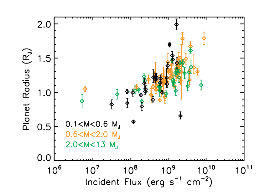
Figure 1.— Observed planetary radius as a function of total incident flux for the known transiting gas giants. Planets are plotted in three colors for three different mass cuts. Kepler-12b is shown as a black filled circle. Note the general trend towards smaller radii with decreased insolation. There is a probable break in slope at incident fluxes of $1-2\sim 10^{8}$erg cm^-2 s^-1. Planets are taken from the compilation at: http://www.inscience.ch/transits/.

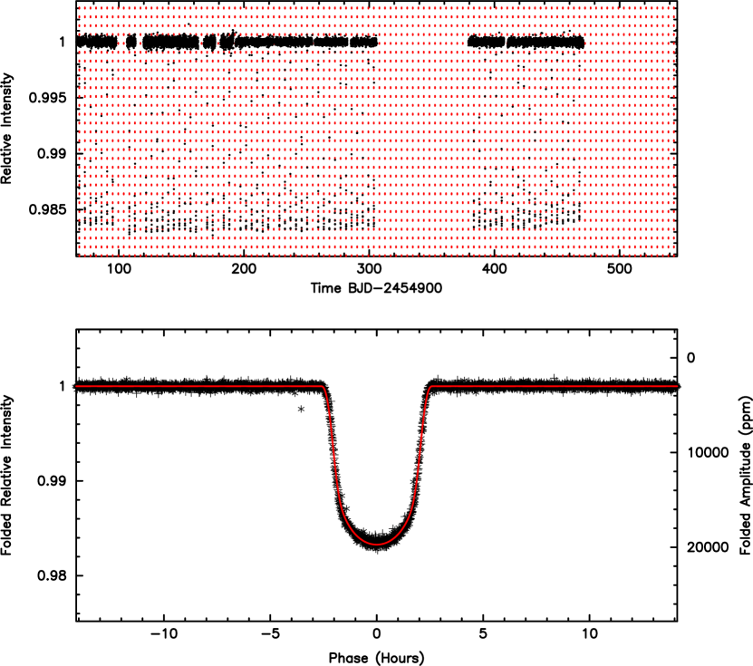
Figure 2.— Time series and folded transit light curve for Kepler-12b.

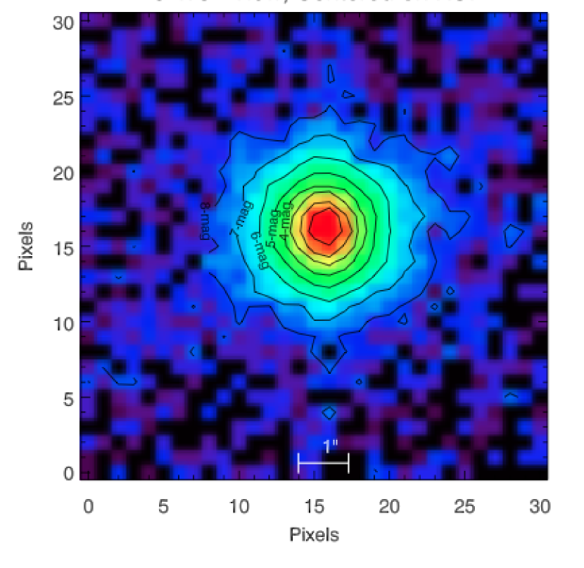
Figure 3.— Image of Kepler-12 taken with the Keck 1 telescope guide camera, showing $9\times 9$ arcsec taken in 0.8 arcsec seeing. North is up and east is to the left and the pixels are 0.30 arcsec in size. The exposure time was 1.0 sec. The detector is a Photometrics CCD and the filter is a BG38, making the passband roughly 400 - 800 nm, similar to that of Kepler. Contours show surface brightness relative to the core. No companion is seen down to 7 magnitudes fainter than Kepler-12 beyond $\sim$1 arcsec from it. There is no evidence of a star that could be an eclipsing binary.

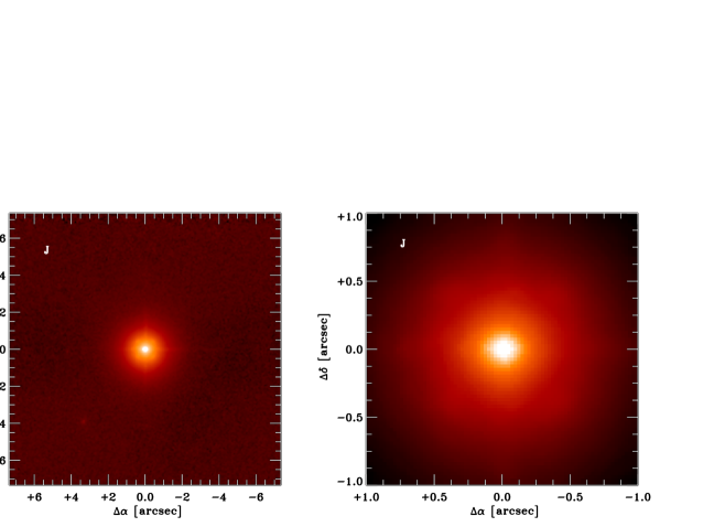
Figure 4.— $J$ Palomar adaptive optics image of Kepler-12. The left image displays a $15^{\prime\prime}\times 15^{\prime\prime}$ field of view centered on the primary target. The right image displays a $2^{\prime\prime}\times 2^{\prime\prime}$ field of view centered on the primary target. The four-point pattern surrounding the central point spread function core is part of the adaptive optics point spread function.

Figure 5.— Palomar detection limits as a function of radial distance from the primary target, Kepler-12. The filled circles represent the J-band limits and each point represents a step in FWHM away from the primary target centroid peak. The dashed line underneath represents the J-band limits converted to Kepler magnitude limits if a star were to have a nominal $m_{Kepler}-J$ color. (For a magnitude limited sample, the median $m_{Kepler}-J$ = $1.28\pm 0.52$).

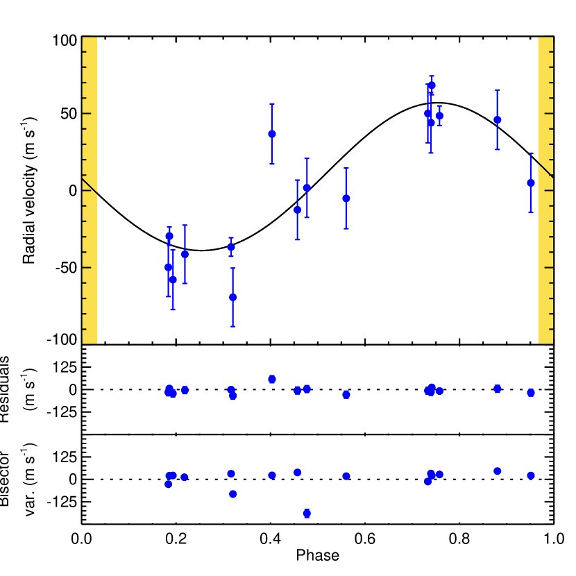
Figure 6.— (a) Orbital solution for Kepler-12b. The observed radial velocities obtained with HIRES on the Keck Telescope are plotted together with the velocity curve for a circular orbit with the period and time of transit fixed by the photometric ephemeris. The radial velocities have an arbitrary zero point. (b) Velocity residuals from the orbital solution. The rms of the velocity residuals is $24~{}\rm{m\,s^{-1}}$. (c) Variation in the bisector spans for HIRES spectra. The zero point is arbitrary and the RMS is $59~{}\rm{m\,s^{-1}}$.

Figure 7.— Five stellar evolution models from the Yonsei-Yale (Y²) grids. From left to right the lines show 1.4, 1.3, 1.2, 1.1 and 1.0 $M_{\odot}$ models for Z=0.0206, which is appropriate given this parent star’s metallicity, relative to the solar abundances used in the Y² grids. The boxes show the 68.3, 95.4, 99.73% confidence intervals on the stellar $T_{\rm eff}$ and $\bar{\rho_{\star}}$ as determined by spectroscopy and transit model fits. The ’hook’ in the evolution tracks for more massive stars with convective cores produces a non-uniform distribution of masses with the uncertainty boxes and can produce a degeneracy in the solution for the best-fit stellar parameters.

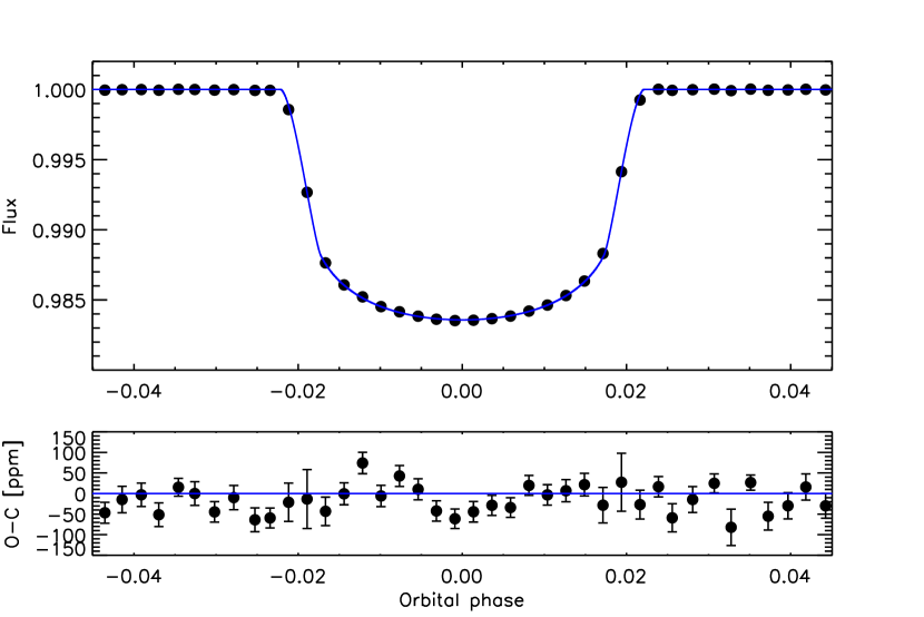
Figure 8.— Top: Kepler-12 b phase-folded transit lightcurve with best-fit model superimposed. The data are binned in 15 minute intervals. Error bars are smaller than the plotted datapoints. Bottom: residuals are displayed in parts per million (ppm) scale.

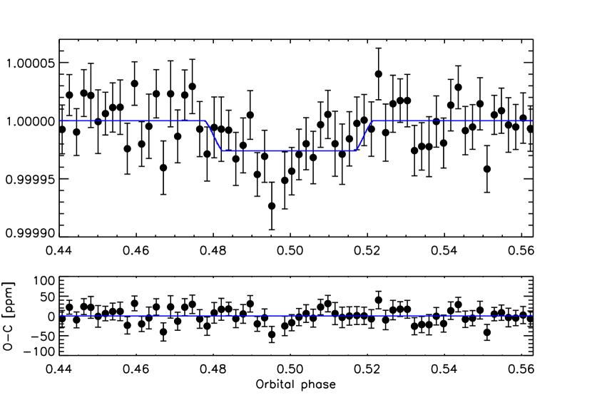
Figure 9.— Top: Kepler-12 b phase-folded occultation lightcurve with best-fit model superimposed. The Kepler data are binned in 15 minute increments. Bottom: residuals are displayed in parts per million (ppm) scale.

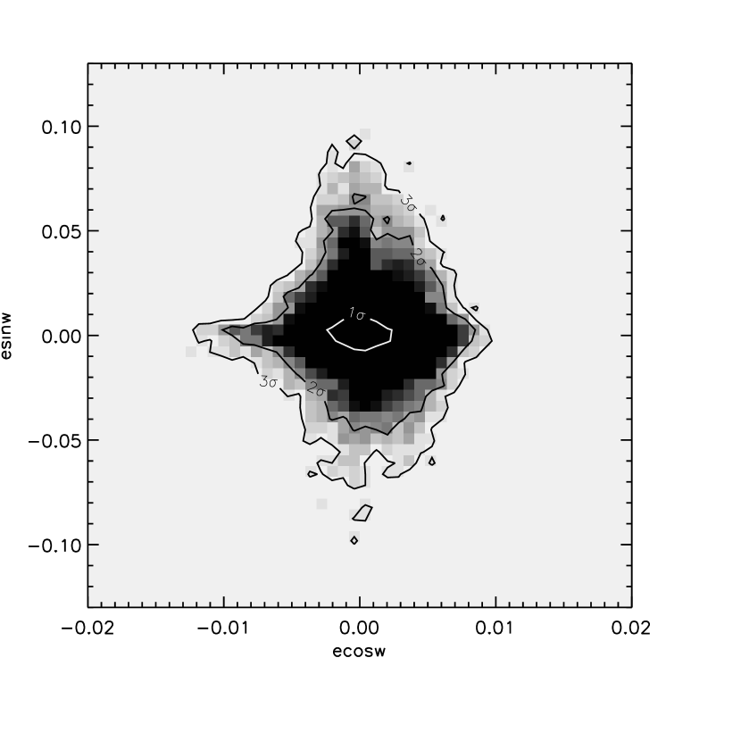
Figure 10.— Density function of the two-dimensional $e\sin\omega$/$e\cos\omega$ successful MCMC trials (density increases from white to black). Note the different scales for x and y axes. The 1, 2 and 3$\sigma$ confidence domains are superimposed. The weak constraint from the occultation duration leads to a significant scatter in $e\sin\omega$. As $e\cos\omega$ is well constrained from the occultation timing obtained by the Kepler and Spitzer photometry, this yields orbital eccentricities as high as $\sim~{}0.09$ (3$\sigma$ upper limit) provided the argument of periastron is close to 90 or 270 degrees. In this case, the eccentricity vector points toward or away of the observer, allowing a wide range of $e\sin\omega$ values while leaving $e\cos\omega$ almost unchanged.

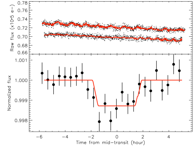
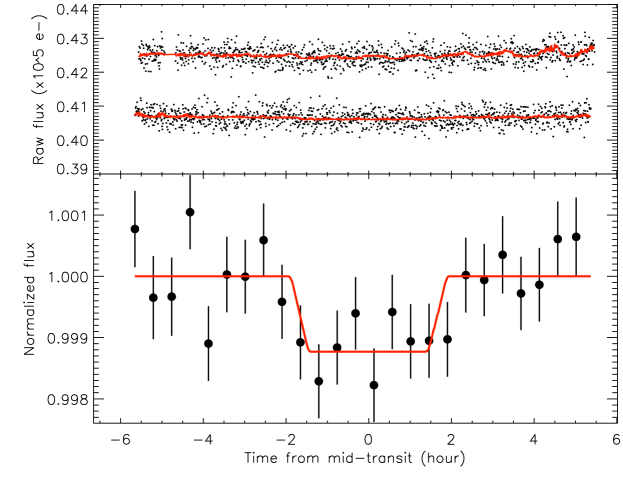
Figure 11.— Spitzer occultation light-curves of Kepler-12b observed in the IRAC band-pass at 3.6 (top) and 4.5 µm (bottom). Top panels: raw and unbinned light-curves. The red solid lines correspond to the best fit models which include the time and position instrumental decorrelations as well as the model for the planetary transit (see details in Sect. 5.1). Bottom panels: corrected and normalized occultation light-curve with the best fit model (in red). The data are binned in 25 minutes intervals (50 points).

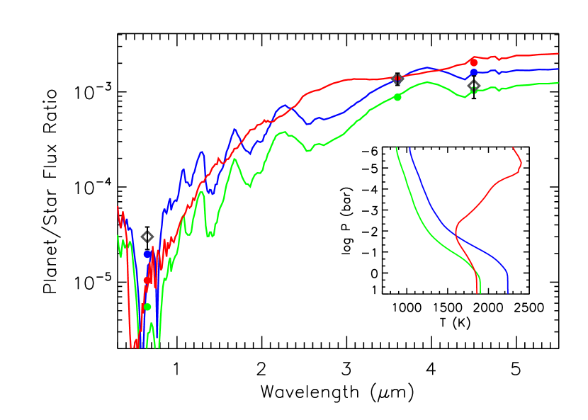
Figure 12.— Main Panel: Planet-to-star flux ratios observed by Kepler and Spitzer, shown in gray. The flux ratios from three planetary models are shown for comparison. There is preference towards models that have no temperature inversion (blue and green). Model ratios integrated over the appropriate bandpasses are shown as filled circles. The Kepler occultation point strongly argues for inefficient redistribution of flux, or an additional scattering component at optical wavelengths. Inset Panel: Atmospheric pressure-temperature profiles for the three models.

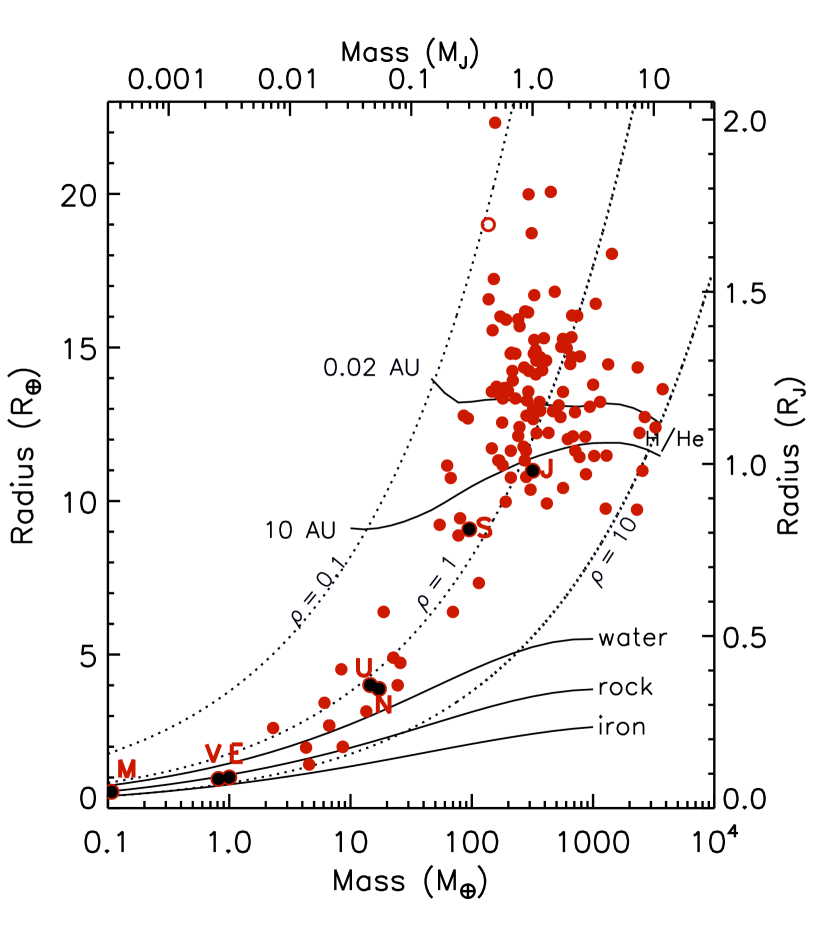
Figure 13.— Mass vs. radius for planets with “well-defined parameters,” as taken from http://www.inscience.ch/transits/, but also including the Kepler-11 system (Lissauer et al., 2011). Kepler-12b is shown as an open circle, the 2nd-lowest density planet discovered. Models (solid black curves) are taken from Fortney et al. (2007). The two upper curves are for pure H-He planets, at 4.5 Gyr, at 0.02 and 10 AU from the Sun.

Table 1 Relative radial velocity and bisector span variation measurements of Kepler-12.

BJD	RV	$\sigma_{\rm RV}$	BS	$\sigma_{\rm BS}$
	($\rm{m~{}s^{-1}}$)	($\rm{m~{}s^{-1}}$)	($\rm{m~{}s^{-1}}$)	($\rm{m~{}s^{-1}}$)
$2455014.91234$	$-12.5$	$19.3$	$38.3$	$6.1$
$2455016.79104$	$45.9$	$19.3$	$46.2$	$6.7$
$2455017.10568$	$5.0$	$19.1$	$21.1$	$3.4$
$2455019.11155$	$36.7$	$19.4$	$22.3$	$4.8$
$2455027.05631$	$-57.9$	$19.4$	$21.5$	$4.6$
$2455041.99855$	$-5.1$	$19.7$	$17.6$	$5.9$
$2455042.79449$	$44.0$	$19.6$	$32.3$	$4.6$
$2455073.83165$	$50.0$	$19.1$	$-12.1$	$2.9$
$2455075.83091$	$-49.8$	$19.0$	$-27.0$	$2.9$
$2455080.87564$	$-69.3$	$19.0$	$-81.8$	$9.1$
$2455084.86254$	$-41.4$	$18.9$	$11.7$	$4.4$
$2455134.82606$	$1.7$	$19.2$	$-189.6$	$22.1$
$2455437.78012$	$68.3$	$6.1$	$21.0$	$3.5$
$2455439.75382$	$-29.6$	$6.0$	$20.2$	$3.7$
$2455759.86617$	$-36.6$	$6.0$	$31.4$	$3.8$
$2455761.82490$	$48.5$	$6.4$	$27.1$	$4.1$

Table 2Kepler-12 system parameters

Parameters	Value
Jump parameters
Planet/star area ratio $(R_{p}/R_{s})^{2}$	$0.013765^{+0.000020}_{-0.000020}$
$b^{\prime}=a\cos i/R_{\star}$ [$R_{\star}$]	$0.174^{+0.011}_{-0.011}$
Transit width [d]	$0.19573^{+0.00009}_{-0.00010}$
$T_{0}$ - 2450000 [HJD]	$5004.00835^{+0.00002}_{-0.00002}$
Orbital period $P$ [d]	$4.4379637^{+0.0000002}_{-0.0000002}$
RV $K^{\prime}$ [m s-1 d1/3]	$79.2^{+7.1}_{-7.0}$
$\sqrt{e}\cos\omega$	$-0.001^{+0.054}_{-0.051}$
$\sqrt{e}\sin\omega$	$0.001^{+0.097}_{-0.114}$
$c_{1}=2u_{1}+u_{2}$	$1.009^{+0.005}_{-0.005}$
$c_{2}=u_{1}-2u_{2}$	$-0.182^{+0.016}_{-0.014}$
Occultation depth	$0.000031^{+0.000007}_{-0.000007}$
Deduced stellar parameters
$u_{1}$	$0.367^{+0.003}_{-0.003}$
$u_{2}$	$0.274^{+0.006}_{-0.006}$
Density $\rho_{\star}$ [$\rho_{\odot}$]	$0.354^{+0.017}_{-0.008}$
Surface gravity $\log g_{\star}$ [cgs]	$4.175^{+0.015}_{-0.011}$
Mass $M_{\star}$ [$M_{\odot}$]	$1.166^{+0.051}_{-0.054}$
Radius $R_{\star}$ [$R_{\odot}$]	$1.483^{+0.025}_{-0.029}$
Age [Gyr]	$4.0^{+0.3}_{-0.4}$
Observed stellar parameters
$T_{\rm eff}$	$5947\pm 100$
$\mathrm{[Fe/H]}$	$0.07\pm 0.04$
$V\rm{sin}$$i$	$0.8\pm 0.5$ km s-1
Deduced planet parameters
RV $K$ [m s-1]	$48.2^{+4.4}_{-4.3}$
$b_{transit}$ [$R_{\star}$]	$0.174^{+0.011}_{-0.011}$
$b_{occultation}$ [$R_{\star}$]	$0.174^{+0.011}_{-0.011}$
$T_{occultation}$ - 2450000 [HJD]	$5010.666^{+0.004}_{-0.003}$
Orbital semi-major axis $a$ [AU]	$0.0556^{+0.0007}_{-0.0007}$
Orbital inclination $i$ [deg]	$88.76^{+0.08}_{-0.08}$
Orbital eccentricity $e$	$<0.01$ (1$\sigma$), $<0.09$ (3$\sigma$)
Argument of periastron $\omega$ [deg]	$182^{+97}_{-98}$
Density $\rho_{P}$ [g cm-3]	$0.111^{+0.011}_{-0.009}$
Surface gravity log $g_{P}$ [cgs]	$2.57^{+0.04}_{-0.04}$
Mass $M_{P}$ [$M_{Jup}$]	$0.431^{+0.041}_{-0.040}$
Radius $R_{P}$ [$R_{Jup}$]	$1.695^{+0.028}_{-0.032}$

Table 3Warm-Spitzer observations.

Visit	AOR	Wavelength	Obs. Date (UT)	Select. points	Depth (%)	Weighted. Avg. depth	$T_{\rm bright}$
1	40251392	3.6	2010-09-06	1233	$0.141^{+0.026}_{-0.021}$	-	-
3	40250880	3.6	2010-12-26	1151	$0.130^{+0.026}_{-0.032}$	$0.137\pm 0.020$%	$1597\pm 160$ K
2	40251136	4.5	2010-09-15	1160	$0.108^{+0.046}_{-0.034}$	-	-
4	40250624	4.5	2011-01-08	1212	$0.129^{+0.039}_{-0.061}$	$0.116\pm 0.031$%	$1429\pm 190$ K

References

- Ackerman & Marley (2001) Ackerman, A. S., & Marley, M. S. 2001, ApJ, 556, 872
- Anderson et al. (2010) Anderson, D. R., et al. 2010, ApJ, 709, 159
- Anderson et al. (2011) —. 2011, ApJ, 726, L19+
- Arras & Socrates (2010) Arras, P., & Socrates, A. 2010, ApJ, 714, 1
- Baraffe et al. (2008) Baraffe, I., Chabrier, G., & Barman, T. 2008, A&A, 482, 315
- Baraffe et al. (2010) —. 2010, Reports on Progress in Physics, 73, 016901
- Barnes (2007) Barnes, J. W. 2007, PASP, 119, 986
- Batygin & Stevenson (2010) Batygin, K., & Stevenson, D. J. 2010, ApJ, 714, L238
- Batygin et al. (2011) Batygin, K., Stevenson, D. J., & Bodenheimer, P. H. 2011, ApJ, 738, 1
- Beerer et al. (2011) Beerer, I. M., et al. 2011, ApJ, 727, 23
- Bodenheimer et al. (2000) Bodenheimer, P., Hubickyj, O., & Lissauer, J. J. 2000, Icarus, 143, 2
- Bodenheimer et al. (2003) Bodenheimer, P., Laughlin, G., & Lin, D. N. C. 2003, ApJ, 592, 555
- Borucki et al. (2010) Borucki, W. J., et al. 2010, Science, 327, 977
- Borucki et al. (2011) —. 2011, ApJ, 728, 117
- Burrows et al. (2007) Burrows, A., Hubeny, I., Budaj, J., & Hubbard, W. B. 2007, ApJ, 661, 502
- Burrows et al. (2008) Burrows, A., Ibgui, L., & Hubeny, I. 2008, ApJ, 682, 1277
- Burrows et al. (1997) Burrows, A., et al. 1997, ApJ, 491, 856
- Carlin & Lewis (2008) Carlin, B. P., & Lewis, B. P. 2008, Bayesian Methods for Data Analysis
- Chabrier & Baraffe (2007) Chabrier, G., & Baraffe, I. 2007, ApJ, 661, L81
- Charbonneau et al. (2007) Charbonneau, D., Brown, T. M., Burrows, A., & Laughlin, G. 2007, in Protostars and Planets V, ed. B. Reipurth, D. Jewitt, & K. Keil, 701–716
- Charbonneau et al. (2000) Charbonneau, D., Brown, T. M., Latham, D. W., & Mayor, M. 2000, ApJ, 529, L45
- Charbonneau et al. (2005) Charbonneau, D., et al. 2005, ApJ, 626, 523
- Claret & Bloemen (2011) Claret, A., & Bloemen, S. 2011, A&A, 529, A75+
- Cowan & Agol (2011) Cowan, N. B., & Agol, E. 2011, ApJ, 729, 54
- Demarque et al. (2004) Demarque, P., Woo, J.-H., Kim, Y.-C., & Yi, S. K. 2004, ApJS, 155, 667
- Deming et al. (2005) Deming, D., Seager, S., Richardson, L. J., & Harrington, J. 2005, Nature, 434, 740
- Deming et al. (2011) Deming, D., et al. 2011, ApJ, 726, 95
- Désert et al. (2009) Désert, J., Lecavelier des Etangs, A., Hébrard, G., Sing, D. K., Ehrenreich, D., Ferlet, R., & Vidal-Madjar, A. 2009, ApJ, 699, 478
- Désert et al. (2011a) Désert, J., et al. 2011a, ArXiv:1102.0555
- Désert et al. (2011b) —. 2011b, A&A, 526, A12+
- Fazio et al. (2004) Fazio, G. G., et al. 2004, ApJS, 154, 10
- Ford et al. (2011) Ford, E. B., et al. 2011, ArXiv:1102.0544
- Fortney et al. (2008) Fortney, J. J., Lodders, K., Marley, M. S., & Freedman, R. S. 2008, ApJ, 678, 1419
- Fortney & Marley (2007) Fortney, J. J., & Marley, M. S. 2007, ApJ, 666, L45
- Fortney et al. (2007) Fortney, J. J., Marley, M. S., & Barnes, J. W. 2007, ApJ, 659, 1661
- Fortney et al. (2005) Fortney, J. J., Marley, M. S., Lodders, K., Saumon, D., & Freedman, R. 2005, ApJ, 627, L69
- Fortney & Nettelmann (2010) Fortney, J. J., & Nettelmann, N. 2010, Space Sci. Rev., 152, 423
- Fortney et al. (2006) Fortney, J. J., Saumon, D., Marley, M. S., Lodders, K., & Freedman, R. S. 2006, ApJ, 642, 495
- Fortney et al. (2003) Fortney, J. J., Sudarsky, D., Hubeny, I., Cooper, C. S., Hubbard, W. B., Burrows, A., & Lunine, J. I. 2003, ApJ, 589, 615
- Freedman et al. (2008) Freedman, R. S., Marley, M. S., & Lodders, K. 2008, ApJS, 174, 504
- Gelman & Rubin (1992) Gelman, A., & Rubin, D. 1992, Statistical Science, 7, 457
- Gilliland et al. (2010) Gilliland, R. L., et al. 2010, ApJ, 713, L160
- Gillon et al. (2009) Gillon, M., et al. 2009, A&A, 506, 359
- Gillon et al. (2010) —. 2010, A&A, 511, A3+
- Goody et al. (1989) Goody, R., West, R., Chen, L., & Crisp, D. 1989, Journal of Quantitative Spectroscopy and Radiative Transfer, 42, 539
- Guillot et al. (1996) Guillot, T., Burrows, A., Hubbard, W. B., Lunine, J. I., & Saumon, D. 1996, ApJ, 459, L35
- Guillot & Havel (2011) Guillot, T., & Havel, M. 2011, A&A, 527, A20+
- Guillot et al. (2006) Guillot, T., Santos, N. C., Pont, F., Iro, N., Melo, C., & Ribas, I. 2006, A&A, 453, L21
- Guillot & Showman (2002) Guillot, T., & Showman, A. P. 2002, A&A, 385, 156
- Hayward et al. (2001) Hayward, T. L., Brandl, B., Pirger, B., Blacken, C., Gull, G. E., Schoenwald, J., & Houck, J. R. 2001, PASP, 113, 105
- Hebb et al. (2009) Hebb, L., et al. 2009, ApJ, 693, 1920
- Henry et al. (2000) Henry, G. W., Marcy, G. W., Butler, R. P., & Vogt, S. S. 2000, ApJ, 529, L41
- Holman et al. (2006) Holman, M. J., et al. 2006, ApJ, 652, 1715
- Howell et al. (2011) Howell, S. B., Everett, M. E., Sherry, W., Horch, E., & Ciardi, D. R. 2011, AJ, 142, 19
- Hubeny et al. (2003) Hubeny, I., Burrows, A., & Sudarsky, D. 2003, ApJ, 594, 1011
- Ibgui & Burrows (2009) Ibgui, L., & Burrows, A. 2009, ApJ, 700, 1921
- Jackson et al. (2008) Jackson, B., Greenberg, R., & Barnes, R. 2008, ApJ, 681, 1631
- Jenkins et al. (2010a) Jenkins, J. M., et al. 2010a, ApJ, 724, 1108
- Jenkins et al. (2010b) —. 2010b, ApJ, 713, L120
- Jenkins et al. (2010c) —. 2010c, ApJ, 713, L87
- Kipping (2010) Kipping, D. M. 2010, MNRAS, 408, 1758
- Knutson et al. (2008) Knutson, H. A., Charbonneau, D., Allen, L. E., Burrows, A., & Megeath, S. T. 2008, ApJ, 673, 526
- Knutson et al. (2010) Knutson, H. A., Howard, A. W., & Isaacson, H. 2010, ApJ, 720, 1569
- Knutson et al. (2009) Knutson, H. A., et al. 2009, ApJ, 690, 822
- Koch et al. (2010) Koch, D. G., et al. 2010, ApJ, 713, L79
- Kovács et al. (2010) Kovács, G., et al. 2010, ApJ, 724, 866
- Latham et al. (2011) Latham, D. W., et al. 2011, ApJ, 732, L24+
- Laughlin et al. (2011) Laughlin, G., Crismani, M., & Adams, F. C. 2011, ApJ, 729, L7+
- Lissauer et al. (2011) Lissauer, J. J., et al. 2011, Nature, 470, 53
- Lodders (1999) Lodders, K. 1999, ApJ, 519, 793
- Lodders (2003) —. 2003, ApJ, 591, 1220
- Lodders & Fegley (2002) Lodders, K., & Fegley, B. 2002, Icarus, 155, 393
- Lodders & Fegley (2006) —. 2006, Astrophysics Update 2 (Springer Praxis Books, Berlin: Springer, 2006)
- Mandel & Agol (2002) Mandel, K., & Agol, E. 2002, ApJ, 580, L171
- Mandushev et al. (2007) Mandushev, G., et al. 2007, ApJ, 667, L195
- Markwardt (2009) Markwardt, C. B. 2009, in Astronomical Society of the Pacific Conference Series, Vol. 411, Astronomical Data Analysis Software and Systems XVIII, ed. D. A. Bohlender, D. Durand, & P. Dowler, 251–+
- Marley et al. (2007) Marley, M. S., Fortney, J., Seager, S., & Barman, T. 2007, in Protostars and Planets V, ed. B. Reipurth, D. Jewitt, & K. Keil, 733–747
- Marley et al. (1999) Marley, M. S., Gelino, C., Stephens, D., Lunine, J. I., & Freedman, R. 1999, ApJ, 513, 879
- Marley & McKay (1999) Marley, M. S., & McKay, C. P. 1999, Icarus, 138, 268
- Marley et al. (1996) Marley, M. S., Saumon, D., Guillot, T., Freedman, R. S., Hubbard, W. B., Burrows, A., & Lunine, J. I. 1996, Science, 272, 1919
- Marley et al. (2002) Marley, M. S., Seager, S., Saumon, D., Lodders, K., Ackerman, A. S., Freedman, R. S., & Fan, X. 2002, ApJ, 568, 335
- McKay et al. (1989) McKay, C. P., Pollack, J. B., & Courtin, R. 1989, Icarus, 80, 23
- Miller & Fortney (2011) Miller, N., & Fortney, J. J. 2011, ArXiv:1105.0024
- Miller et al. (2009) Miller, N., Fortney, J. J., & Jackson, B. 2009, ApJ, 702, 1413
- Pont et al. (2006) Pont, F., Zucker, S., & Queloz, D. 2006, MNRAS, 373, 231
- Press et al. (1992) Press, W. H., Teukolsky, S. A., Vetterling, W. T., & Flannery, B. P. 1992, Numerical recipes in FORTRAN. The art of scientific computing
- Saumon & Marley (2008) Saumon, D., & Marley, M. S. 2008, ApJ, 689, 1327
- Seager & Deming (2010) Seager, S., & Deming, D. 2010, ARA&A, 48, 631
- Seager et al. (2000) Seager, S., Whitney, B. A., & Sasselov, D. D. 2000, ApJ, 540, 504
- Showman & Guillot (2002) Showman, A. P., & Guillot, T. 2002, A&A, 385, 166
- Sozzetti et al. (2009) Sozzetti, A., et al. 2009, ApJ, 691, 1145
- Spiegel & Burrows (2010) Spiegel, D. S., & Burrows, A. 2010, ApJ, 722, 871
- Sudarsky et al. (2003) Sudarsky, D., Burrows, A., & Hubeny, I. 2003, ApJ, 588, 1121
- Sudarsky et al. (2000) Sudarsky, D., Burrows, A., & Pinto, P. 2000, ApJ, 538, 885
- Toon et al. (1989) Toon, O. B., McKay, C. P., Ackerman, T. P., & Santhanam, K. 1989, Journal of Geophysical Research, 94, 16287
- Torres et al. (2011) Torres, G., et al. 2011, ApJ, 727, 24
- Troy et al. (2000) Troy, M., et al. 2000, in Society of Photo-Optical Instrumentation Engineers (SPIE) Conference Series, Vol. 4007, Society of Photo-Optical Instrumentation Engineers (SPIE) Conference Series, ed. P. L. Wizinowich, 31–40
- Vogt et al. (1994) Vogt, S. S., et al. 1994, in Presented at the Society of Photo-Optical Instrumentation Engineers (SPIE) Conference, Vol. 2198, Society of Photo-Optical Instrumentation Engineers (SPIE) Conference Series, ed. D. L. Crawford & E. R. Craine, 362–+
- Werner et al. (2004) Werner, M. W., et al. 2004, ApJS, 154, 1
- Winn et al. (2008) Winn, J. N., et al. 2008, ApJ, 683, 1076
- Wright et al. (2009) Wright, J. T., Upadhyay, S., Marcy, G. W., Fischer, D. A., Ford, E. B., & Johnson, J. A. 2009, ApJ, 693, 1084
- Wright et al. (2011) Wright, J. T., et al. 2011, PASP, 123, 412
- Youdin & Mitchell (2010) Youdin, A. N., & Mitchell, J. L. 2010, ApJ, 721, 1113