Online Learning for Combinatorial Network Optimization with Restless Markovian Rewards

Abstract

Combinatorial network optimization algorithms that compute optimal structures taking into account edge weights form the foundation for many network protocols. Examples include shortest path routing, minimal spanning tree computation, maximum weighted matching on bipartite graphs, etc. We present CLRMR, the first online learning algorithm that efficiently solves the stochastic version of these problems where the underlying edge weights vary as independent Markov chains with unknown dynamics.

The performance of an online learning algorithm is characterized in terms of regret, defined as the cumulative difference in rewards between a suitably-defined genie, and that obtained by the given algorithm. We prove that, compared to a genie that knows the Markov transition matrices and uses the single-best structure at all times, CLRMR yields regret that is polynomial in the number of edges and nearly-logarithmic in time.

I Introduction

The following abstract description of combinatorial network optimization covers many graph theoretic algorithms that form the basis of network protocol design in wired and wireless networks. Given a graph $G=(V,E)$, where each edge $e\in E$ is associated with a weight $w_{e}$, find a structure consisting of a collection of edges satisfying some given property (e.g., a path, a tree, a matching, or an independent set), that maximizes or minimizes the sum of the weights on the selected edges. This kind of linear network combinatorial optimization covers, for instance, shortest path and minimum spanning tree computation used in routing protocols, and maximum-weight matching used for channel scheduling and switching.

In practice, the edge weights may correspond to some link quality metric of interest such as packet reception ratio, delay, or throughput. In such a case, the edge weights are often stochastically varying with time. Moreover, the dynamics may not be known a priori. The solution approach to this problem that we advocate here is to combine the estimation and optimization phases jointly via an efficient online learning algorithm.

We present in this paper an online learning algorithm that is designed for the setting where the edge weights are modeled by finite-state Markov chains, with unknown transition matrices. We show that this problem can be modeled as a combinatorial multi-armed bandit problem with restless Markovian rewards.

To characterize the performance of this algorithm, following the convention in the multi-armed bandit literature, we define a notion of regret, defined as the difference in reward between a suitably defined model-aware genie and that accumulated by the given algorithm over time. Specifically, in this work, we consider a single-action regret formulation, whereby the genie is assumed to know the transition matrices for all edges, but is constrained to stick with one action (corresponding to a particular network structure) at all times. We prove that our algorithm, which we refer to as CLRMR (Combinatorial Learning with Restless Markov Rewards) achieves a regret that is polynomial in the number of Markov chains (i.e., number of edges), and logarithmic with time. This implies that our learning algorithm, which does not know the transition matrices, asymptotically achieves the maximum time averaged reward possible with any single-action policy, even if that policy is given advanced knowledge of the transition matrices. By contrast, the conventional approach of estimating the mean of each edge weight and then finding the desired network structure via deterministic optimization would incur greater overhead and provide only linearly increasing regret over time, which is not asympotically optimal.

While recent work has shown how to address multi-armed bandits with restless Markovian rewards in the classic non-combinatorial setting [Tekin:restless:infocom], and combinatorial multi-armed bandits in the simpler settings of i.i.d. rewards [Gai:LLR] or rested Markovian rewards [Gai:rested:globecom], this paper is the first to show how to efficiently implement online learning for stochastic combinatorial network optimization when edge weights are dynamically evolving as restless Markovian processes. We perform simulations to evaluate our new algorithm over two combinatorial network optimization problems: stochastic shortest path routing and bipartite matching for channel allocation, and show that its regret performance is substantially better than that of the algorithm presented in [Tekin:restless:infocom], which can handle restless Markovian rewards but does not exploit the dependence between the arms, resulting in a regret that grows exponentially in the number of unknown variables.

The rest of the paper is organized as follows. We first provide a survey of prior work in section II. We then present a formal model of the combinatorial restless multi-armed bandit problems in section III. In section IV, we present our CLRMR policy, and show that it requires only polynomial storage. We present our novel analysis of the regret of CLRMR policy in section V. In section LABEL:sec:app:simulation, we discuss examples and show the numerical simulation results, to show that our proposed policy is widely useful for various interesting combinatorial network optimization problems. We finally conclude our paper in section LABEL:sec:conclusion.

II Related Work

We summarize below the related work, which has treated a) temporally i.i.d. rewards, b) rested Markovian rewards, and c) restless Markovian rewards.

II-A Temporally i.i.d. rewards

Lai and Robbins [Lai:Robbins] wrote one of the earliest papers on the classic non-Bayesian infinite horizon multi-armed bandit problem. They assume $K$ independent arms, each generating rewards that are i.i.d. over time obtained from a distribution that can be characterized by a single-parameter. For this problem, they present a policy that provides an expected regret that is $O(K\log n)$, i.e. linear in the number of arms and asymptotically logarithmic in n. Anantharam et al. extend this work to the case when $M$ simultaneous plays are allowed [Anantharam]. The work by Agrawal [Agrawal:1995] presents easier to compute policies based on the sample mean that also has asymptotically logarithmic regret. The paper by Auer et al. [Auer:2002] that considers arms with nonnegative rewards that are i.i.d. over time with an arbitrary non-parameterized distribution that has the only restriction that it have a finite support. Further, they provide a simple policy (referred to as UCB1), which achieves logarithmic regret uniformly over time, rather than only asymptotically. Our work utilizes a general Chernoff-Hoeffding-bound-based approach to regret analysis pioneered by Auer et al..

Some recent work has shown the design of distributed multiuser policies for independent arms. Motivated by the problem of opportunistic access in cognitive radio networks, Liu and Zhao [Liu:Zhao], Anandkumar et al. [Anandkumar:Infocom:2010, Anandkumar:JSAC], and Gai and Krishnamachari [Gai:decentralized:globecom], have developed policies for the problem of $M$ distributed players operating $N$ independent arms.

Our work in this paper is closest to and builds on the recent work by Gai et al. which introduced combinatorial multi-armed bandits [Gai:LLR]. The formulation in [Gai:LLR] has the restriction that the reward process must be i.i.d. over time. A polynomial storage learning algorithm is presented in [Gai:LLR] that yields regret that is polynomial in users and resources and uniformly logarithmic in time for the case of i.i.d. rewards.

II-B Rested Markovian rewards

There has been relatively less work on multi-armed bandits with Markovian rewards. Anantharam et al. [Anantharam:1987] wrote one of the earliest papers with such a setting. They proposed a policy to pick $m$ out of the $N$ arms each time slot and prove the lower bound and the upper bound on regret. However, the rewards in their work are assumed to be generated by rested (i.e. rewards that only evolve when the arms are selected) Markov chains with transition probability matrices defined by a single parameter $\theta$ with identical state spaces. Also, for the upper bound the result is achieved only asymptotically.

For the case of single users and independent arms, a recent work by Tekin and Liu [Tekin:2010] has extended the results in [Anantharam:1987] relaxing the requirement of a single parameter and identical state spaces across arms. They propose to use UCB1 from [Auer:2002] for the multi-armed bandit problem with rested Markovian rewards and prove a logarithmic upper bound on the regret under some conditions on the Markov chain.

In a recent work by Gai et al. [Gai:rested:globecom], learning policies for combinatorial multi-armed bandits with rested Markovian rewards have been studied. Unlike [Gai:rested:globecom], we adopt a model with restless Markovian rewards, which has much broader applications in many network optimization problems.

II-C Restless Markovian rewards

Restless arm bandits are so named because the arms evolve at each time, changing state even when they are not selected. Work on restless Markovian rewards with single users and independent arms can be found in [Tekin:restless:infocom, Qing:icassp, Qing:ita, Dai:icassp]. In these papers there is no consideration of possible dependencies among arms, as in our work here.

Tekin and Liu [Tekin:restless:infocom] have proposed a RCA policy that achieves logarithmic single-action regret when certain knowledge about the system is known. We use elements of the policy and proof from [Tekin:restless:infocom] in this work, which is however quite different in its combinatorial matching formulation (which allows for dependent arms). Liu et al. [Qing:icassp, Qing:ita] adopted the same problem formulation as in [Tekin:restless:infocom], and proposed a policy named RUCB, achieving a logarithmic single-action regret over time when certain system knowledge is known. They also extend the RUCB policy to achieve a near-logarithmic regret asymptotically when no knowledge about the system is available.

Dai et al. in  [Dai:icassp] adopt a stronger definition of regret: the difference in expected reward compared to a model-aware genie. They develop a policy that yields regret of order arbitrarily close to logarithmic for certain classes of restless bandits with a finite-option structure, such as restless MAB with two states and identical probability transition matrices.

III Problem Formulation

We consider a system with $N$ edges predefined by some application, where time is slotted and indexed by $n$. For each edge $i$ ($1\leq i\leq N$), there is an associated state that evolves as a discrete-time, finite-state, aperiodic, irreducible Markov chain $\{X^{i}(n),n\geq 0\}$ with unknown parameters. We denote the state space for the $i$-th Markov chain by $S^{i}$. We assume these $N$ Markov chains are mutually independent. The reward obtained from state $x$ ($x\in S^{i}$) of Markov chain $i$ is denoted as $r^{i}_{x}$. Denote by $\pi^{i}_{x}$ the steady state distribution for state $x$. The mean reward obtained on Markov chain $i$ is denoted by $\mu^{i}$. Then we have $\mu^{i}=\sum\limits_{z\in S_{i,j}}r^{i}_{x}\pi^{i}_{x}$. The set of all mean rewards is denoted by $\bm{\mu}=\{\mu^{i}\}$.

At each decision period $n$ (also referred to interchangeably as time slot), an $N$-dimensional action vector $\mathbf{a}(n)$, representing an arm, is selected under a policy $\phi(n)$ from a finite set $\mathcal{F}$. We assume $a_{i}(n)\geq 0$ for all $1\leq i\leq N$. When a particular $\mathbf{a}(n)$ is selected, the value of $r^{i}_{x_{i}(n)}$ is observed, only for those $i$ with $a_{i}(n)\neq 0$. We denote by $\mathcal{A}_{\mathbf{a}(n)}=\{i:a_{i}(n)\neq 0,1\leq i\leq N\}$ the index set of all $a_{i}(n)\neq 0$ for an arm $\mathbf{a}$. We treat each $\mathbf{a}(n)\in\mathcal{F}$ as an arm. The reward is defined as:

$$R^{\mathbf{a}(n)}(n)=\sum\limits_{i\in\mathcal{A}_{\mathbf{a}(n)}}a_{i}(n)r^{i}_{x_{i}(n)}$$ (1)

where $x_{i}(n)$ denotes the state of a Markov chain $i$ at time $n$.

When a particular arm $\mathbf{a}(n)$ is selected, the rewards corresponding to non-zero components of $\mathbf{a}(n)$ are revealed, i.e., the value of $r^{i}_{x_{i}(n)}$ is observed for all $i$ such that $a_{i}(n)\neq 0$.

The state of the Markov chain evolves restlessly, i.e., the state will continue to evolve independently of the actions. We denote by $P^{i}=(p^{i}_{x,y})_{x,y\in S^{i}}$ the transition probability matrix for the Markov chain $i$. We denote by $(P^{i})^{\prime}=\{(p^{i})^{\prime}_{x,y}\}_{x,y\in S^{i}}$ the adjoint of $P^{i}$ on $l_{2}(\pi)$, so $(p^{i})^{\prime}_{x,y}=p^{i}_{y,x}\pi^{i}_{y}/\pi^{i}_{x}$. Denote $\hat{P}^{i}=(P^{i})^{\prime}P$ as the multiplicative symmetrization of $P^{i}$. For aperiodic irreducible Markov chains, $\hat{P}^{i}$s are irreducible [Diaconis:1995].

A key metric of interest in evaluating a given policy $\phi$ for this problem is regret, which is defined as the difference between the expected reward that could be obtained by the best-possible static action, and that obtained by the given policy. It can be expressed as:

$$\begin{split}\mathfrak{R}^{\phi}(n)&=n\gamma^{*}-\mathbb{E}^{\phi}[\sum\limits_{t=1}^{n}R^{\phi(t)}(t)]\\ &=n\gamma^{*}-\mathbb{E}^{\phi}[\sum\limits_{t=1}^{n}\sum\limits_{i\in\mathcal{A}_{\mathbf{a}(t)}}a_{i}(t)r^{i}_{x_{i}(t)}]\end{split}$$ (2)

where $\gamma^{*}=\max\limits_{\mathbf{a}\in\mathcal{F}}\sum\limits_{i\in\mathcal{A}_{\mathbf{a}(n)}}a_{i}\mu^{i}$ is the expected reward of the optimal arm. For the rest of the paper, we use $*$ as the index indicating that a parameter is for an optimal arm. If there is more than one optimal arm, $*$ refers to any one of them. We denote by $\gamma^{\mathbf{a}}$ the expected reward of arm $\mathbf{a}$, so $\gamma^{\mathbf{a}}=\sum\limits_{j=1}^{|\mathcal{A}_{\mathbf{a}}|}a_{p_{j}}\mu^{p_{j}}$.

For this combinatorial multi-armed bandit problem with restless Markovian rewards, our goal is to design policies that perform well with respect to regret. Intuitively, we would like the regret $\mathfrak{R}^{\phi}(n)$ to be as small as possible. If it is sublinear with respect to time $n$, the time-averaged regret will tend to zero.

IV Policy Design

For the above combinatorial MAB problem with restless rewards, we have two challenges here for the policy design:

(1) A straightforward idea is to apply RCA in [Tekin:restless:infocom], or RUCB in [Qing:icassp] directly and naively, and ignore the dependencies across the different arms. However, we note that RCA and RUCB both require the storage and computation time that are linear in the number of arms. Since there could be exponentially many arms in this formulation, it is highly unsatisfactory.

(2) Unlike our prior work on combinatorial MAB with rested rewards, for which the transitions only occur each time the Markov chains are observed, the policy design for the restless case is much more difficult, since the current state while starting to play a Markov chain depends not only on the transition probabilities, but also on the policy.

To deal with the first challenge, we want to design a policy which more efficiently stores observations from the correlated arms, and exploits the correlations to make better decisions. Instead of storing the information for each arm, our idea is to use two $1$ by $N$ vectors to store the information for each Markov chain. Then an index for each each arm is calculated, based on the information stored for underlying components. This index is used for choosing the arm to be played each time when a decion needs to be made.

To deal with the second challenge, for each arm $\mathbf{a}$ we note that the multidimensional Markov chain $\{X^{\mathbf{a}}(n),n\geq 0\}$ defined by underlying components as $X^{\mathbf{a}}(n)=(X^{i}(n))_{i\in\mathcal{A}_{\mathbf{a}}}$ is aperiodic and irreducible. Instead of utilizing the actual sample path of all observations, we only take the observations from a regenerative cycle for Markov chains and discard the rest in its estimation of the index.

Our proposed policy, which we refer to as Combinatorial Learning with Restless Markov Reward (CLRMR), is shown in Algorithm 1. Table I summerizes the notation we use for CLRMR algorithm. For Algorithm 1, $(x_{i})_{i\in\mathcal{A}_{\mathbf{a}}}=(\zeta^{i})_{i\in\mathcal{A}_{\mathbf{a}}}$ means $x_{i}=\zeta^{i},\forall i$.

Algorithm 1 Combinatorial Learning with Restless Markov Reward (CLRMR)

1:$//$ Initialization

2:$t=1$, $t_{2}=1$;

3:$\forall i=1,\cdots,N$, $m^{i}_{2}=0$, $\bar{z}^{i}_{2}=0$;

4:for $b=1$ to $N$ do

5:     $t:=t+1$, $t_{2}:=t_{2}+1$;

6:     Play any arm $\mathbf{a}$ such that $b\in\mathcal{A}_{\mathbf{a}}$; denote $(x_{i})_{i\in\mathcal{A}_{\mathbf{a}}}$ as the observed state vector for arm $\mathbf{a}$;

7:     $\forall i\in\mathcal{A}_{\mathbf{a}(n)}$, let $\zeta^{i}$ be the first state observed for Markov chain $i$ if $\zeta^{i}$ has never been set; $\bar{z}^{i}_{2}:=\frac{\bar{z}^{i}_{2}m^{i}_{2}+r^{i}_{x_{i}}}{m^{i}_{2}+1}$, $m^{i}_{2}:=m^{i}_{2}+1$;

8:     while $(x_{i})_{i\in\mathcal{A}_{\mathbf{a}}}\neq(\zeta^{i})_{i\in\mathcal{A}_{\mathbf{a}}}$ do

9:         $t:=t+1$, $t_{2}:=t_{2}+1$;

10:         Play arm $\mathbf{a}$; denote $(x_{i})_{i\in\mathcal{A}_{\mathbf{a}}}$ as the observed state vector;

11:         $\forall i\in\mathcal{A}_{\mathbf{a}(n)}$, $\bar{z}^{i}_{2}:=\frac{\bar{z}^{i}_{2}m^{i}_{2}+r^{i}_{x_{i}}}{m^{i}_{2}+1}$, $m^{i}_{2}:=m^{i}_{2}+1$;

12:     end while

13:end for

14:$//$ Main loop

15:while 1 do

16:     $//$ SB1 starts

17:     $t:=t+1$;

18:     Play an arm $\mathbf{a}$ which maximizes

$$\max\limits_{\mathbf{a}\in\mathcal{F}}\sum\limits_{i\in\mathcal{A}_{\mathbf{a}}}a_{i}\left(\bar{z}^{i}_{2}+\sqrt{\frac{L\ln t_{2}}{m^{i}_{2}}}\right);$$ (3)

19:     Denote $(x_{i})_{i\in\mathcal{A}_{\mathbf{a}}}$ as the observed state vector;

20:     while $(x_{i})_{i\in\mathcal{A}_{\mathbf{a}}}\neq(\zeta^{i})_{i\in\mathcal{A}_{\mathbf{a}}}$ do

21:         $t:=t+1$;

22:         Play an arm $\mathbf{a}$ and denote $(x_{i})_{i\in\mathcal{A}_{\mathbf{a}}}$ as the observed state vector;

23:     end while

24:     $//$ SB2 starts

25:     $t_{2}:=t_{2}+1$;

26:     $\forall i\in\mathcal{A}_{\mathbf{a}(n)}$, $\bar{z}^{i}_{2}:=\frac{\bar{z}^{i}_{2}m^{i}_{2}+r^{i}_{x_{i}}}{m^{i}_{2}+1}$, $m^{i}_{2}:=m^{i}_{2}+1$;

27:     while $(x_{i})_{i\in\mathcal{A}_{\mathbf{a}}}\neq(\zeta^{i})_{i\in\mathcal{A}_{\mathbf{a}}}$ do

28:         $t:=t+1$, $t_{2}:=t_{2}+1$;

29:         Play an arm $\mathbf{a}$ and denote $(x_{i})_{i\in\mathcal{A}_{\mathbf{a}}}$ as the observed state vector;

30:         $\forall i\in\mathcal{A}_{\mathbf{a}(n)}$, $\bar{z}^{i}_{2}:=\frac{\bar{z}^{i}_{2}m^{i}_{2}+r^{i}_{x_{i}}}{m^{i}_{2}+1}$, $m^{i}_{2}:=m^{i}_{2}+1$;

31:     end while

32:     $//$ SB3 is the last play in the while loop. Then a block completes.

33:     $b:=b+1$, $t:=t+1$;

34:end while

$N$ :	number of resources
$\mathbf{a}$:	vectors of coefficients, defined on set $\mathcal{F}$;
	we map each $\mathbf{a}$ as an arm
$\mathcal{A}_{\mathbf{a}}$:	$\{i:a_{i}\neq 0,1\leq i\leq N\}$
$t$:	current time slot
$t_{2}$:	number of time slots in SB2 up to the current
	time slot
$b$:	number of blocks up to the current time slot
$m^{i}_{2}$:	number of times that Markov chain $i$ has been
	observed during SB2 up to the current time slot
$\bar{z}^{i}_{2}$:	average (sample mean) of all the observed
	values of Markov chain $i$ during SB2 up to
	the current time slot
$\zeta^{i}$:	state that determine the regenerative cycles for
	Markov chain $i$
$x_{i}$:	the observed state when Markov Chain $i$ is
	played; $(x_{i})_{i\in\mathcal{A}_{\mathbf{a}}}$ is the observed state vector
	if arm $\mathbf{a}$ is played

TABLE I: Notation for Algorithm 1

CLRMR operates in blocks. Figure 1 illustrates one possible realization of this Algorithm 1. At the beginning of each block, an arm $\mathbf{a}$ is picked and within one block, this algorithm always play the same arm. For each Markov chain $\{X^{i}(n)\}$, we specifiy a state $\zeta^{i}$ at the beginning of the algorithm as a state to mark the regenerative cycle. Then, for the multidimentional Markov chain $\{X^{\mathbf{a}}(n)\}$ associated with this arm, the state $(\zeta^{i})_{i\in\mathcal{A}_{\mathbf{a}}}$ is used to define a regenerative cycle for $\{X^{\mathbf{a}}(n)\}$.

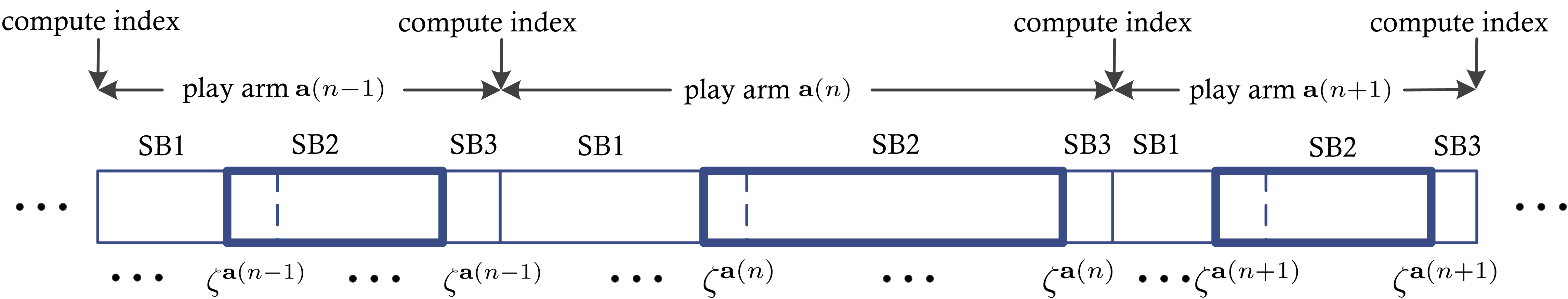
Figure 1: An illustration of CLRMR

Each block is broken into three sub-blocks denoted by SB1, SB2 and SB3. In SB1, the selected arm $\mathbf{a}$ is played until the state $(\zeta^{i})_{i\in\mathcal{A}_{\mathbf{a}}}$ is observed. Upon this observation we enter a regenerative cycle, and continue playing the same arm untill $(\zeta^{i})_{i\in\mathcal{A}_{\mathbf{a}}}$ is observed again. SB2 includes all time slots from the first visit of $(\zeta^{i})_{i\in\mathcal{A}_{\mathbf{a}}}$ up to but excluding the second visit to $(\zeta^{i})_{i\in\mathcal{A}_{\mathbf{a}}}$. SB3 consists a single time slot with the second visit to $(\zeta^{i})_{i\in\mathcal{A}_{\mathbf{a}}}$. SB1 is empty if the first observed state is $(\zeta^{i})_{i\in\mathcal{A}_{\mathbf{a}}}$. So SB2 includes the observed rewards for a regenerative cycle of the multidimentional Markov chain $\{X^{\mathbf{a}}(n)\}$ associated with arm $\mathbf{a}$, which implies that SB2 also includes the observed rewards for one or more regenerative cycles for each underlying Markov chain $\{X^{i}(n)\},i\in\mathcal{A}_{\mathbf{a}}$.

The key to the algorithm 1 is to store the observations for each Markov chain instead of the whole arm, and utilize the observations only in SB2 for them, and virtually assemble them (highlighted with thick lines in Figure 1). Due to the regenerative nature of the Markov chain, by putting the observations in SB2, the sample path has exactly the same statics as given by the transition probability matrix. So the problem is tractable.

LLR policy requires storage linear in $N$. We use two $1$ by $N$ vectors to store the information for each Markov chain after we play the selected arm at each time slot in SB2. One is $(\bar{z}^{i}_{2})_{1\times N}$ in which $\bar{z}^{i}_{2}$ is the average (sample mean) of observed values in SB2 up to the current time slot (obtained through potentially different sets of arms over time). The other one is $(m^{i}_{2})_{1\times N}$ in which $m^{i}_{2}$ is the number of times that $\{X^{i}(n)\}$ has been observed in SB2 up to the current time slot.

Line 1 to line 13 are the initialization, for which each Markov chain is observed at least once, and $\zeta^{i}$ is specified as the first state observed for $\{X^{i}(n)\}$.

After the initialization, at the beginning of each block, CLRMR selects the arm which solves the maximization problem as in (3). It is a deterministic linear optimal problem with a feasible set $\mathcal{F}$ and the computation time for an arbitrary $\mathcal{F}$ may not be polynomial in $N$. But, as we show in Section LABEL:sec:app:simulation, there exist many practically useful examples with polynomial computation time.

V Analysis of Regret

We summarize some notation we use in the description and analysis of our CLRMR policy in Table II.

$H$ :	$\max\limits_{\mathbf{a}}|\mathcal{A}_{\mathbf{a}}|$. Note that $H\leq N$
$\mathbf{a}(\tau)$ :	the arm played in time $\tau$
$b(n)$:	number of completed blocks up to time $n$
$t(b)$:	time at the end of block $b$
$t_{2}(b)$:	total number of time slots spent in SB2
	up to block $b$
$B^{\mathbf{a}}(b)$:	total number of blocks within the first $b$
	blocks in which arm $\mathbf{a}$ is played
$m^{i}_{2}(t_{2}(b))$: total number of time slots Markov chain $i$
	is observed during SB2 up to block $b$
$\bar{z}^{i}_{2}(s)$:	the mean reward from Markov chain $i$
	when it is observed for the $s$-th time of
	only those times played during SB2
$T(n)$:	time at the end of the last completed block
$T^{\mathbf{a}}(n)$:	total number of time slots arm $\mathbf{a}$ is palyed
	up to time $T(n)$
$m^{i}_{x}(s)$:	number of times that state $x$ occured when
	Markov chain $i$ has been observed $s$ times
$Y^{i}_{1}(j)$:	vector of observed states from SB1 of the
	$j$-th block for playing Markov chain $i$
$Y^{i}_{2}(j)$:	vector of observed states from SB2 of the
	$j$-th block for playing Markov chain $i$
$Y^{i}(j)$:	vector of observed states from the $j$-th
	block for playing Markov chain $i$
$\hat{\pi}^{i}_{x}$:	$\max\{\pi^{i}_{x},1-\pi^{i}_{x}\}$
$\hat{\pi}_{\max}$:	$\max\limits_{i,x\in S^{i}}\hat{\pi}^{i}_{x}$
$\pi_{\min}$:	$\min\limits_{i,x\in S^{i}}\pi^{i}_{x}$
$\pi_{\max}$:	$\max\limits_{i,x\in S^{i}}\pi^{i}_{x}$
$\epsilon^{i}$:	eigenvalue gap, defined as $1-\lambda_{2}$, where
	$\lambda_{2}$ is the second largest eigenvalue of the
	multiplicative symmetrization of $P^{i}$
$\epsilon_{\min}$:	$\min\limits_{i}\epsilon^{i}$
$S_{\max}$:	$\max\limits_{i}|S^{i}|$
$r_{\max}$:	$\max\limits_{i,x\in S^{i}}r^{i}_{x}$
$a_{\max}$:	$\max\limits_{i\in\mathcal{A}_{\mathbf{a}},\mathbf{a}\in\mathcal{F}}a_{i}$
$\Delta_{\mathbf{a}}$:	$\gamma^{*}-\gamma^{\mathbf{a}}$
$\Delta_{\min}$:	$\min\limits_{\gamma^{\mathbf{a}}\leq\gamma^{*}}\Delta_{\mathbf{a}}$
$\Delta_{\max}$:	$\max\limits_{\gamma^{\mathbf{a}}\leq\gamma^{*}}\Delta_{\mathbf{a}}$
$\{X^{\mathbf{a}}(n)\}$: multidimentional Markov chain defined
	by $X^{\mathbf{a}}(n)=(X^{i}(n))_{i\in\mathcal{A}_{\mathbf{a}}}$
$\zeta^{\mathbf{a}}$:	$(\zeta^{i})_{i\in\mathcal{A}_{\mathbf{a}}}$, state vector that determines
	the regenerative cycles for $\{X^{\mathbf{a}}(n)\}$
$\Pi^{\mathbf{a}}_{z}$:	steady state distribution for state $z$ of $\{X^{\mathbf{a}}(n)\}$
$\Pi^{\mathbf{a}}_{\min}$:	$\min\limits_{z\in S^{\mathbf{a}}}\Pi^{\mathbf{a}}_{z}$
$\Pi_{\min}$:	$\min\limits_{\mathbf{a},z\in S^{\mathbf{a}}}\Pi^{\mathbf{a}}_{z}$
$M^{\mathbf{a}}_{z_{1},z_{2}}$:	mean hitting time of state $z_{2}$ starting
	from an initial state $z_{1}$ for $\{X^{\mathbf{a}}(n)\}$
$M^{\mathbf{a}}_{\max}$:	$\max\limits_{z_{1},z_{2}\in S^{\mathbf{a}}}M^{\mathbf{a}}_{z_{1},z_{2}}$
$\gamma^{\prime}_{\max}$:	$\max\limits_{\gamma^{\mathbf{a}}\leq\gamma^{*}}\gamma^{\mathbf{a}}$

TABLE II: Notation for Regret Analysis

We first show in Theorem 1 an upper bound on the total expected number of plays of suboptimal arms.

Theorem 1

When using any constant $L\geq 56(H+1)S^{2}_{\max}r^{2}_{\max}\hat{\pi}^{2}_{\max}/\epsilon_{\min}$, we have

$$\sum\limits_{\mathbf{a}:\gamma^{\mathbf{a}}<\gamma^{*}}(\gamma^{*}-\gamma^{\mathbf{a}})\mathbb{E}[T^{\mathbf{a}}(n)]\leq Z_{1}\ln n+Z_{2}$$

where

$$Z_{1}=\Delta_{\max}\left(\frac{1}{\Pi_{\min}}+M_{\max}+1\right)\frac{4NLH^{2}a_{\max}^{2}}{\Delta^{2}_{\min}}$$

$$Z_{2}=\Delta_{\max}\left(\frac{1}{\Pi_{\min}}+M_{\max}+1\right)\left(N+\frac{\pi NHS_{\max}}{3\pi_{\min}}\right)$$

To proof Theorem 1, we use the inequalities as stated in Theorem 3.3 from [lezaud] and a theorem from [bremaud].

Lemma 1 (Theorem 3.3 from [lezaud])

Consider a finite-state, irreducible Markov chain $\left\{X_{t}\right\}_{t\geq 1}$ with state space $S$, matrix of transition probabilities $P$, an initial distribution $\mathbf{q}$ and stationary distribution $\mathbf{\pi}$. Let $N_{\mathbf{q}}=\left\|(\frac{q_{x}}{\pi_{x}},x\in S)\right\|_{2}$. Let $\hat{P}=P^{\prime}P$ be the multiplicative symmetrization of $P$ where $P^{\prime}$ is the adjoint of $P$ on $l_{2}(\pi)$. Let $\epsilon=1-\lambda_{2}$, where $\lambda_{2}$ is the second largest eigenvalue of the matrix $\hat{P}$. $\epsilon$ will be referred to as the eigenvalue gap of $\hat{P}$. Let $f:S\rightarrow\mathcal{R}$ be such that $\sum_{y\in S}\pi_{y}f(y)=0$, $\left\|f\right\|_{\infty}\leq 1$ and $0<\left\|f\right\|^{2}_{2}\leq 1$. If $\hat{P}$ is irreducible, then for any positive integer $n$ and all $0<\delta\leq 1$

$$P\left(\frac{\sum_{t=1}^{n}f(X_{t})}{n}\geq\delta\right)\leq N_{q}\exp\left[-\frac{n\delta^{2}\epsilon}{28}\right]~{}.$$