Light cone effect on the reionization 21-cm power spectrum
Abstract
Observations of redshifted 21-cm radiation from neutral hydrogen during the epoch of reionization (EoR) are considered to constitute the most promising tool to probe that epoch. One of the major goals of the first generation of low frequency radio telescopes is to measure the 3D 21-cm power spectrum. However, the 21-cm signal could evolve substantially along the line of sight (LOS) direction of an observed 3D volume, since the received signal from different planes transverse to the LOS originated from different look-back times and could therefore be statistically different. Using numerical simulations we investigate this so-called light cone effect on the spherically averaged 3D 21-cm power spectrum. For this version of the power spectrum, we find that the effect mostly ‘averages out’ and observe a smaller change in the power spectrum compared to the amount of evolution in the mean 21-cm signal and its rms variations along the LOS direction. Nevertheless, changes up to at large scales are possible. In general the power is enhanced/suppressed at large/small scales when the effect is included. The cross-over mode below/above which the power is enhanced/suppressed moves toward larger scales as reionization proceeds. When considering the 3D power spectrum we find it to be anisotropic at the late stages of reionization and on large scales. The effect is dominated by the evolution of the ionized fraction of hydrogen during reionization and including peculiar velocities hardly changes these conclusions. We present simple analytical models which explain qualitatively all the features we see in the simulations.
keywords:
cosmology: theory, cosmology: diffuse radiation, cosmology: reionization, methods: numerical, methods: statistical1 Introduction
The epoch of reionization (EoR), when the first luminous sources reionized the neutral hydrogen in the intergalactic medium (IGM), is currently the frontier of observational astronomy. Observations of the Cosmic Microwave Background Radiation (CMBR) (Komatsu et al., 2011; Larson et al., 2011) and high redshift quasar absorption spectra (Becker et al., 2001; Fan et al., 2006; Willott et al., 2009) jointly suggest that reionization took place over an extended period spanning the redshift range (see e.g. Mitra et al., 2011). Observations of high redshift Ly -emitting galaxies (Malhotra & Rhoads, 2004; Ouchi et al., 2010; Kashikawa et al., 2011) and gamma ray bursts (Totani et al., 2006) are also consistent with this picture.
Observations of redshifted 21-cm radiation are considered to constitute the most promising tool to probe the EoR (for a review see Furlanetto et al., 2006). For the past few years substantial efforts have been undertaken both on the theoretical and experimental side (reviewed in Morales & Wyithe, 2010). The first generation of low frequency radio telescopes ( GMRT111http://gmrt.ncra.tifr.res.in/, LOFAR222http://www.lofar.org/, MWA333Lonsdale et al. (2009), http://www.mwatelescope.org, PAPER444Parsons et al. (2010)) is either operational or will be operational very soon. Preliminary results from these facilities include foreground measurements at EoR frequencies (Ali et al., 2008; Bernardi et al., 2009; Pen et al., 2009; Paciga et al., 2010) as well as some constraints on reionization (Bowman & Rogers, 2010; Paciga et al., 2010).
Motivated by the detection possibility of the EoR 21-cm signal and the subsequent science results, a wide range of efforts are ongoing on the theoretical side with the goal to understand the physics of reionization and its expected 21-cm signal. Furlanetto et al. (2004) developed analytical models to calculate the ionized bubble size distribution and use this for calculating the 21-cm power spectrum. Such models are very useful in predicting the signal quickly for a wide range of scales and investigating the large parameter space. However, they cannot incorporate details of reionization and become less accurate when the bubbles start overlapping. Numerical simulations are probably the best way to predict the expected 21-cm signal. Although challenging, there has been considerable progresses in simulating the large scale 21-cm signal during the entire EoR (Iliev et al., 2006; Mellema et al., 2006a; McQuinn et al., 2007; Shin et al., 2008; Baek et al., 2009). More approximate but much faster semi-numerical simulations of the structure and evolution of reionization and the 21-cm signal have also been developed (Zahn et al., 2007; Mesinger & Furlanetto, 2007; Santos et al., 2008; Geil & Wyithe, 2008; Thomas et al., 2009; Choudhury et al., 2009). These methods are capable of generating volumes with sizes as large as (Alvarez et al., 2009; Santos et al., 2010). Many aspects such as source properties, feed back effects, distribution and properties of sinks have also been investigated in detail (see Trac & Gnedin, 2009, for a review on reionization simulations).
One of the major goals of all first generation EoR telescopes is to measure the spherically averaged 3D 21-cm power spectrum. Measurements of the 21-cm power spectrum will provide a wealth of information about the timing and duration of reionization, large scale distribution of H I and its evolution, source properties and clustering (Ali et al., 2005; Sethi, 2005; Datta et al., 2007; Lidz et al., 2008; Barkana, 2009). To obtain the spherically averaged 3D power spectrum one needs to average over the 3D volume produced by the observations. Of this 3D volume one axis (the LOS axis) is along the frequency direction. Since light from the lower frequency side of the 3D volume takes a longer time to reach us than light from the high frequency side, the observer will see reionization in an earlier phase at the lower frequency side than at the higher frequency side. The statistics of 21-cm fluctuations could therefore be changing over the observed volume. As we will see in section 2 and 3, in some reionization scenarios the change could be substantial especially near the end of reionization. Almost all previous studies calculate the 3D 21-cm power spectrum without taking this effect into account. In this paper we investigate the effect of LOS evolution or the so called ‘light cone’ effect on the measured 21-cm power spectrum, using numerical simulations to quantify it. Understanding the light cone effect is important because it will be present in the data and needs to be taken into account when interpreting the observed 21-cm power spectrum. Our aim is to understand under which conditions and at what scales this effect needs to be considered.
The light cone effect is well known from studies of galaxy clustering (see e.g. Matsubara et al., 1997). In the context of 21-cm studies of reionization it was first considered by Barkana & Loeb (2006). These authors studied analytically the anisotropic structure of the two point correlation function caused by the effect. This appears to be only work that considered the effect of a changing source population. However, more work has been done on the light cone effect for a single bright source, such as a QSO. For this case the effect will make the H II region appear to be teardrop-shaped (Wyithe et al., 2005; Yu, 2005; Majumdar et al., 2010). The effects on the power spectrum and correlation function for this case were investigated by Sethi & Haiman (2008). In addition, for very luminous sources the effect of relativistically expanding H II regions (Shapiro et al., 2006) would have to be added to the one purely due to evolution of the signal along the LOS.
Bright QSOs are quite rare, so the more common form of the light cone effect will be due to the evolving source population and the growing H II regions around groups of sources. Our aim is to study this version of the effect on the spherically averaged 3D and the 1D LOS power spectra using realistic numerical simulations of reionization.
The paper is organized as follows. Section 2 briefly describes our simulations and the procedure used to generate light cone cubes. We present our results in Section 3. Section 4 describes two simple toy models which explain qualitatively the main features we see in the simulation results. Section 5 investigates how the inclusion of peculiar velocities affect our results. We summarize our results and conclusions in Section 6. The cosmological parameters we use throughout the paper are and , consistent with the WMAP seven-year results (Komatsu et al., 2011).
2 Simulation
2.1 The redshifted 21-cm signal
The 21-cm radiation is emitted when neutral hydrogen atoms go through spin-flip transitions. The radiation can be decoupled from the cosmic microwave background (CMB) photons either through collisions with hydrogen atoms and free electrons (Purcell & Field, 1956; Field, 1959; Zygelman, 2005) or through Ly photon pumping (Wouthuysen, 1952; Field, 1959; Chen & Miralda-Escudé, 2004; Hirata, 2006; Chuzhoy & Shapiro, 2006). This makes 21-cm radiation detectable either in emission or absorption against the CMB. The differential brightness temperature with respect to the CMB is commonly written using the spin temperature as
| (1) |
where and are the mass averaged neutral fraction and the density fluctuations of hydrogen. Note that the 21-cm signal remains undetectable when the spin temperature is coupled to the CMB temperature . During the EoR, is expected to be coupled to the gas kinetic temperature through Ly photon coupling. In addition the gas kinetic temperature is expected to be much higher than the CMB temperature due to heating by shocks, X-rays and Ly photons. This would make the redshifted 21-cm signal visible in emission. We assume here that which makes the 21-cm signal independent of the actual value of . This is a reasonable assumption during the later stages of the EoR. During the initial stages of reionization, when there are few sources of radiation, this assumption might not hold (Baek et al., 2010; Thomas & Zaroubi, 2011). The next subsection describes how we simulate the fluctuations in the H I density.
2.2 N-Body and radiative transfer runs
Details about our simulation methodology (N-body simulation and the subsequent radiative transfer) have been presented in previous papers (Iliev et al., 2006; Mellema et al., 2006a; Iliev et al., 2007, 2011). Iliev et al. (2011) described the simulations we use here in more detail. Here we only present a brief overview of the major features of these simulations.
We start by simulating the evolution of the dark matter distribution using the CubeP3M N-body code in a comoving volume of using particles and cells. This implies particle masses of and a minimum resolvable halo mass of which approximately matches the minimum mass of haloes able to cool by atomic cooling. The N-body simulations give the DM density field, locations and masses of haloes. We then assume that the baryons trace the DM density field and assign an ionizing photon luminosity to each halo assuming it to be proportional to the halo mass,
| (2) |
where is the number of ionizing photons emitted per time. and are the halo mass and proton mass respectively. The efficiency parameter can be written as,
| (3) |
where is the number of ionizing photons emitted into the IGM per baryon per star forming episode (which is taken to be the same as simulation time-step, about years). This makes the factor the product of the escape fraction of ionizing radiation , the star formation efficiency , and the number of ionizing photons produced per baryon for a given initial mass function (IMF), . The latter number is around 5,000 for a Salpeter IMF and times higher for top heavy IMFs, and the two fractions are of the order 10%. This gives values in the range 1 to 100. We divide the halos into low mass atomically cooling halos of mass – M⊙ and high mass atomically cooling halos of masses higher than that. To take into account feedback on the low mass halos, we turn off their ionizing luminosity when they are located in an ionized region.
We then calculate the transfer of ionizing photons with the C2-Ray code (Mellema et al., 2006b) on a grid. Ionizing photons are traced from every source cell to every grid cell within a given time step. This gives us the distribution of the H I fraction in the volume at different redshifts.
Here we consider three cases for the ionizing photon luminosity. In the first simulation, labeled L1 in Iliev et al. (2011), or for sources of mass M⊙ and or for sources of mass between M⊙. In the second simulation, labeled L2, these factors are or and or . In the third case, labelled L3, sources of mass below M⊙ have been turned off. To end reionization at almost the same time as L1, the active sources have been assigned a higher luminosity with or . This particular setup was chosen to make it analogous to the older simulations from Iliev et al. (2008), but updated for the WMAP5 cosmology.
The simulations L1 and L3 are the ones which have the strongest evolution, where L3 due to the lack of low mass sources has the fastest evolution. Since the light cone effect is caused by evolution, below we will focus on these two cases and briefly mention the more slowly evolving case L2 at the end of Section 3.
2.3 Light cone cube
The simulations provide us with so-called ‘coeval cubes’, 3D volumes of density and H I fraction at the same cosmological redshift. The extent of these cubes corresponds to a redshift range of , depending on redshift. An observer can not observe these coeval cubes, but we use them to create observable ‘light cone’ cubes. The procedure which was previously introduced in Mellema et al. (2006a), is as follows:
-
•
From the simulation we obtain a set of coeval 21-cm cubes at redshifts each of integer size and physical comoving size . For the case at hand and cMpc.
-
•
Starting at we create a redshift series of length () which will constitute the redshift (LOS) axis of the light cone ‘cube’ (which will therefore not be cubical). Each consecutive redshift in the series is the same comoving distance apart, namely .
-
•
We then construct the light cone cube by stepping through this redshift series and constructing the 21-cm slices of size for each redshift.
-
•
To create the th 21-cm slice of the light cone cube, we first calculate the integer division and its remainder . We pick up the th slice from the two coeval cubes at and , where , and use linear interpolation in redshift to create an 21-cm slice at .
We should point out that the light cone cubes constructed this way differ from the observational ones in that the field of view has a constant comoving size and not a constant angular size. This is a natural consequence of the way they are constructed from the simulation results and makes it easier to construct the 3D power spectra from them. For the real interferometric observations the angular field of view would be slowly changing as a function of frequency and the physical comoving size depends on the redshift via the angular-size distance relationship. For determining the 3D 21-cm power spectrum in -space it will always be possible to extract a volume with a constant comoving field of view from the observational data.
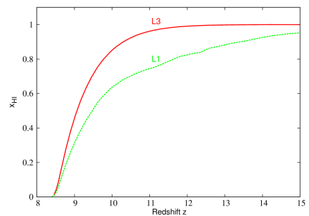
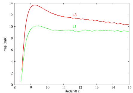
From the L1 simulation we extracted 35 coeval cubes at redshifts spanning from to . In this model reionization starts earlier with the mass weighted ionization fraction reaching and around redshifts and respectively (see Figure 1). In the L3 model, where the smaller mass halos do not contribute, the reionization process starts later (because massive sources form later) and the and points are reached around redshifts and respectively. By construction, the two simulations complete reionization at the same redshift of 8.4, so in the L3 simulation reionization proceeds faster. Because L3 has fewer sources, the characteristic bubble size for a given neutral fraction is bigger. Both models are consistent with the recent CMB measurements of the electron scattering optical depth. Figure 1 shows the evolution of the mass averaged neutral fraction (left panel) and the rms of 21-cm fluctuations (right panel) for the two models. Note that for L3 the rms is higher than for L1 because of the larger ionized bubbles which amplify the rms signal.
Since the comoving distance between to is larger than 163 cMpc our full light cone cube is constructed by using the periodicity of our cosmological volume. However, this does mean that we pass through the same structures several times and our power spectra would be unphysical below scales of Mpc-1. We therefore limit our power spectrum analysis to subvolumes of LOS size 163 cMpc, which roughly corresponds to a frequency depth of MHz.
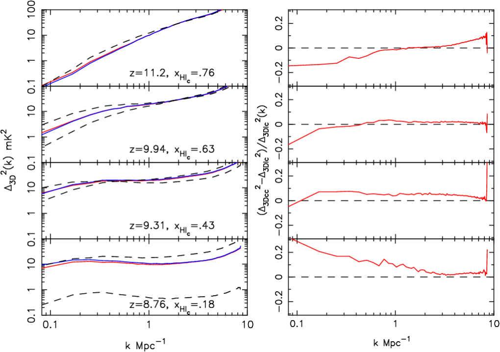
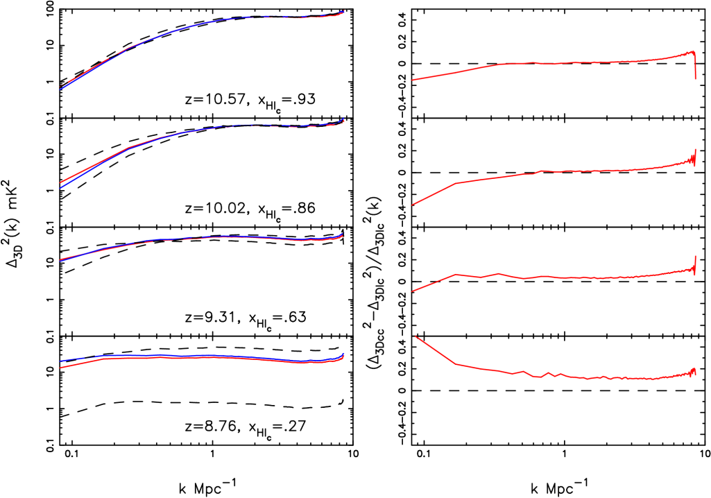
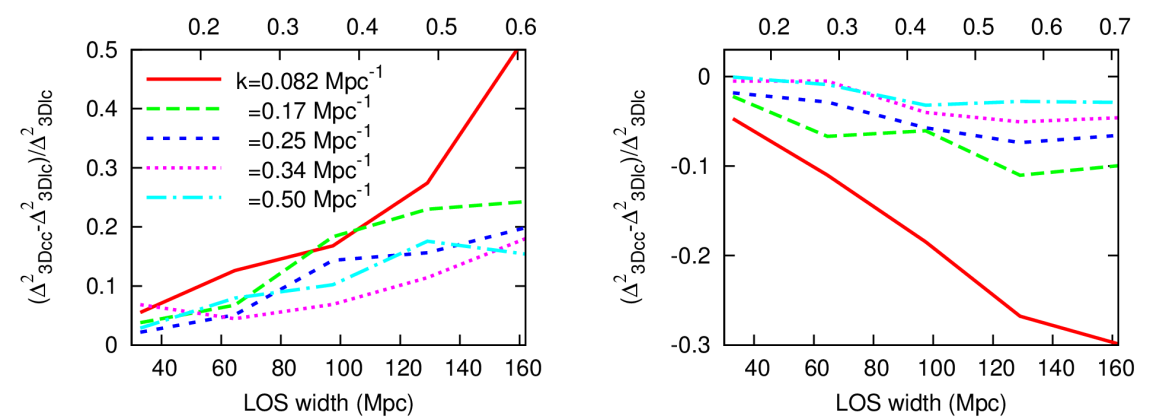
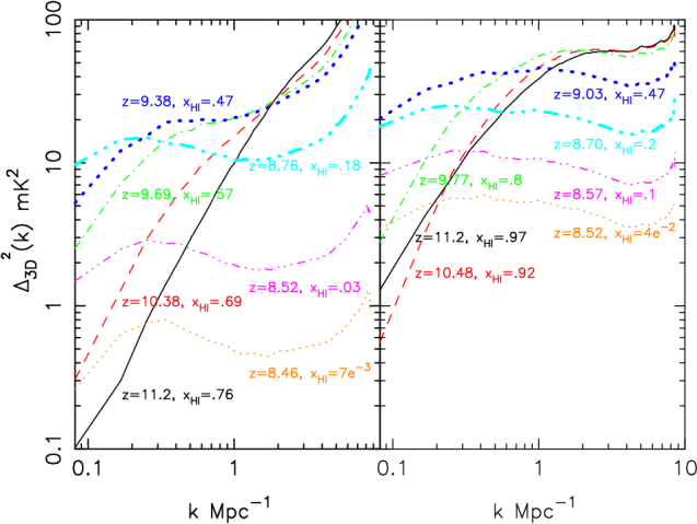
Figure 2 shows the dimensionless spherically averaged 3D 21-cm power spectra (Peacock, 1999) for coeval cubes at different redshifts for both simulations. In the beginning of reionization the power spectrum is dominated by the density fluctuations and quite similar to the underlying dark matter power spectrum. As reionization proceeds the growing ionized bubbles add power at larger scales. When reionization reaches the power reaches a maximum at larger scales. As the neutral fraction goes down further the overall amplitude of the power spectrum also goes down. Note once again that the L3 simulation has more power than the L1 model because of the larger ionized bubbles. From Figure 2 we see the power spectrum evolve both in amplitude and in slope (see Lidz et al., 2008, for a detailed discussion on the power spectrum evolution). The details of the evolution depend on the reionization scenario (for example, the evolution is much faster in the L3 model). If we consider L1, we can see that the power spectrum at changes from to in the redshift range to . Such rapid evolution of the power spectrum (by a factor of at ) within provided the motivation for studying the light cone effect.
3 Effect of evolution
3.1 Spherically averaged power spectrum
| Redshift | rms | |||
| extent | variation | variation | ||
| (mK) | ||||
| 8.76 | ||||
| 9.31 | ||||
| 9.94 | ||||
| 11.2 |
| Redshift | rms | |||
| extent | varies from | varies from | ||
| (mK) | ||||
| 8.76 | ||||
| 9.31 | ||||
| 10.02 | ||||
| 10.57 |
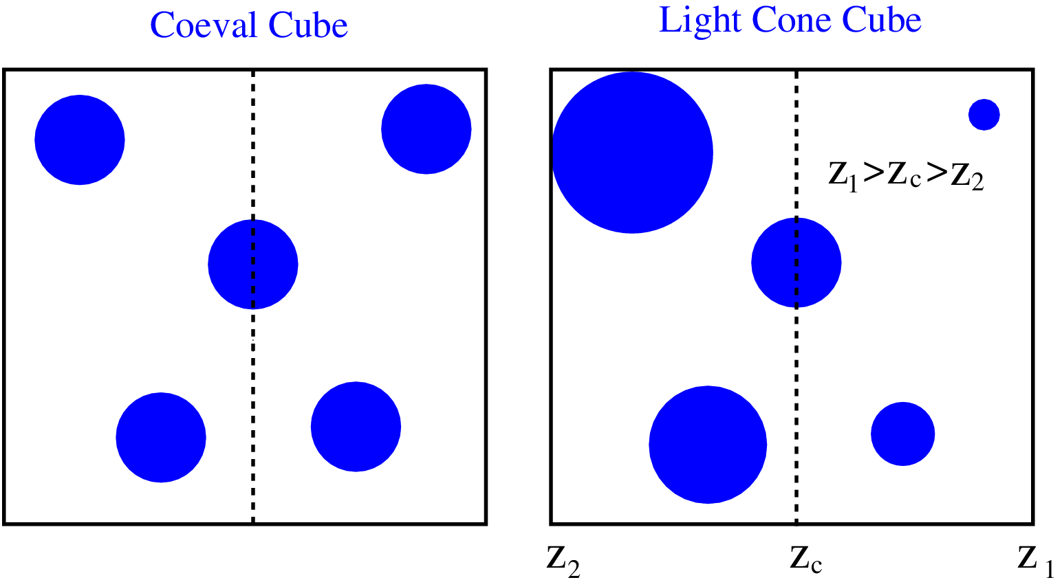
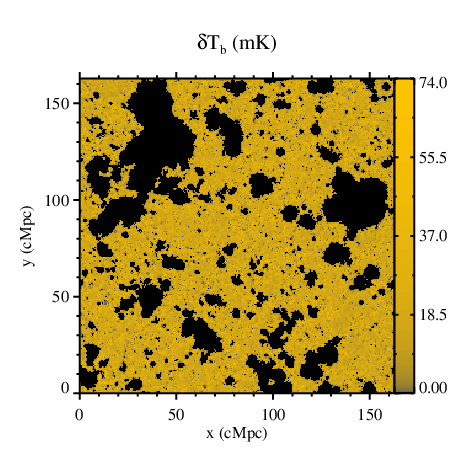
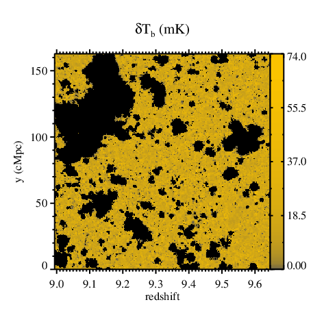
In this section we present and discuss our results on the light cone effect. Figure 3 shows two 21-cm images constructed from simulation L1, the left one from a coeval cube at , and the right one from a light cone cube, where the horizontal axis corresponds to the LOS direction and the central redshift is . We see that ionized regions (black patches) at the higher side (righthand side) are smaller in the light cone image than in the coeval image. Conversely, the ionized regions at the lower end (lefthand side) are larger in the light cone cube.
Figures 4 (for L1) and 5 (for L3) show the effect of evolution on the spherically averaged 3D 21-cm power spectrum. Note that we do not include the modes when we take spherical average over all modes between and . Since we are performing this analysis in the context of radio-interferometric measurements that do not measure the modes , it is appropriate not to include those modes. It is in fact quite important for the analysis we present. Excluding the modes changes the 3D power spectrum from the light cone cube considerably. We discuss this more extensively in Appendix A.
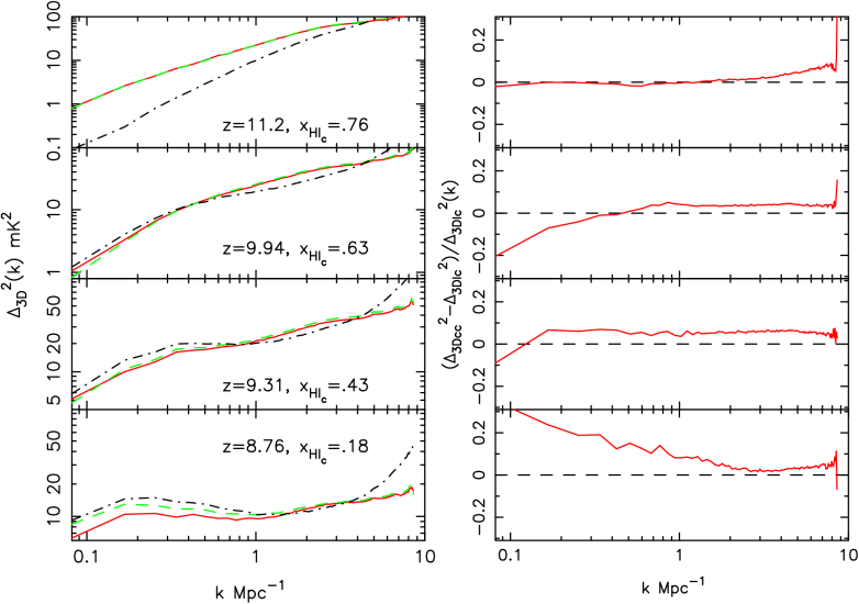
Details about the central redshift (), mass averaged neutral fraction at the central redshift (), redshift range, neutral fraction range and the range of the rms variations in the 21-cm signal for the different light cone cubes from simulations L1 and L3 are given in Tables 1 and 2 respectively. The left panels of Figure. 4 show the spherically averaged 3D power spectra for light cone cubes at four different central redshifts. For comparison it also shows the power spectra for coeval cubes at three redshifts (high, low redshift end and central redshift of the light cone cube). The righthand panels plot the relative difference in the power spectra between the coeval cube at the central redshift and the light cone cube. General features we see in all panels are that the effect is stronger on large scales and increases as we go up in scale. In addition, we find that the power is enhanced (suppressed) with respect to the coeval cube at large (small) scales for neutral fractions . During the last phase of reionization (bottom panels) the power in the light cone cube is suppressed at all scales. At redshift we see that the power spectrum is enhanced by at modes and suppressed by at small scales. At redshift we do not see much effect except on the largest scale where the power is larger by . This is rather surprising since the evolution of the 21-cm signal is stronger in this redshift interval than in the band. For the cube centered around redshift the neutral fraction and the rms change from to and to mK and the power spectrum is amplified by a factor of at (see Table 1 and the last two left panels of Figure 4), much more than what we see in the cube around . So we would expect a larger effect than what we see in Figure 4 at . This trend continues and we see almost no effect for redshift where the neutral fraction and the rms change even more ( and mK) and the power spectrum is amplified by a factor of at Mpc-1. At redshift , instead of an enhancement we see suppression on all scales with differences up to . In the L3 simulation this suppression is up to at redshift . All other features are quite similar in the L3 model (Figure 5) even though the reionization process proceeds faster and the ionized regions are larger in this model.
Another way to describe the trend we see is that we find a cross-over mode below which power is enhanced and above which it is suppressed. The cross-over scales shifts towards lower as the reionization proceeds. At the end of reionization the cross-over mode is lower than the lowest mode we measure from the simulation box.
3.2 Light cone effect as a function of LOS width
Above we present results using the entire cubes i.e, for a LOS width corresponding to the size of our simulation volume. However, it is interesting to explore how the effect changes as one reduces the LOS width. Obviously in the limit of small widths, the light cone effect will disappear, so considering a range a widths allows us to study how it varies with width.
Here we consider sub-boxes of different LOS widths and calculate the quantity for different modes. Figure 6 shows as a function of LOS width (and ) for different modes at two central redshifts and for the L3 simulation. As expected, we see that the quantity decreases for smaller LOS width (and ). As discussed later in the subsection 4.3, we expect the quantity to increase quadratically with the LOS width. However, due to the smaller number of modes available for the smaller , the results are too noisy to test this expectation, although they are roughly consistent with it.
We do not show results for the other two central redshifts of L3 and L1 simulation as the light cone effect is relatively smaller for these, but find similar results there. These results suggest that measurements of the light cone effect for different LOS widths can, in principle, be used to correct for the effect or at least find the sign of the effect.
3.3 Anisotropies in the power spectrum
The light cone effect introduces an anisotropy in the full 3D 21 cm power spectrum. For a fixed -mode, the power spectrum will depend on , the LOS component of . Peculiar velocities and the Alcock-Paczynski effect are the other major sources of anisotropies in the 21 cm power spectrum. In order to understand the anisotropic power spectrum and to separate the physics from astrophysics (Barkana & Loeb, 2005) each effect should be studied in detail. Though the first generation of low frequency radio telescopes (i.g, LOFAR, GMRT, MWA ) are unlikely to able to measure the anisotropies in the 21 cm power spectrum, this will be the ultimate goal of such measurements.
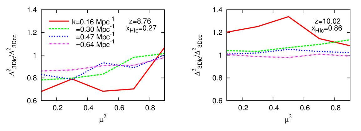
Fig. 7 plots the ratio as a function of for different -modes for two central redshifts (left panel) and (right panel) for L3 simulations. Here . In the left panel () we see that the ratio increases from (at ) to (at ) for . For , the ratio increases from to for the same range. For higher -modes the degree of anisotropy decreases and the power spectrum is becoming more isotropic. We do not see any significant anisotropies for the central redshift (right panel) where the neutral fraction . The other redshifts of the L3 simulation also do not show significant anisotropies and the results for the L1 simulation are similar to L3.
We do not try to quantify the anisotropies further as we see the curves are not very smooth due to the small number of modes at large . Our results are sample variance limited and should be considered as qualitative rather than quantitative. Larger simulation volumes are needed to quantify the anisotropies more precisely. Barkana & Loeb (2006) (fig. 2) reported significant anisotropies at large scales () for neutral fraction in their Pop III reionization model. This is qualitatively consistent with our results.
3.4 1D LOS power spectrum
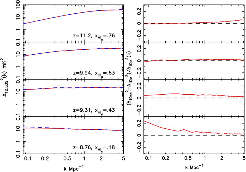
Recent results by Harker et al. (2010) show that the dimensionless 1D LOS power spectrum 555 (Peacock, 1999) can be extracted more accurately as there is no large scale bias (which may arise due to foreground subtraction) and smaller error bars in the recovered 1D LOS power spectrum (shown in figure 11 of Harker et al., 2010). The 1D LOS power spectrum can also extend to smaller scales because of the higher resolution in the frequency direction. Motivated by this, we also study the effect of evolution on the 1D LOS power spectrum. Figure 8 shows the effect in the 1D LOS power spectrum for the L1 case. Interestingly, the 1D LOS power spectrum is hardly affected by light cone effects, except near the end of reionization. We do not show results for the L3 simulation as these are very similar to L1. This result adds one more advantage to the strategy of measuring 1D LOS power spectrum. However, the 1D LOS power spectrum is very flat on large scales due to the aliasing of high -modes. Therefore, although it can be more accurately measured, it may be difficult to see the impact of ionized bubbles and extract the reionization physics.
We would like to mention here that besides the simulations L1, L3 we also analysed the L2 simulation (for more details see Iliev et al., 2011) where the reionization is much more gradual and overlap happens at a redshift . The evolution is thus relatively slow and we see that the light cone effect is smaller in amplitude but otherwise has similar features as what we presented above for the cases L1 and L3.
3.5 Comparison to previous work
Barkana & Loeb (2006) analytically studied the light cone effect using the two point correlation function , rather than considering the power spectrum. Since they considered different reionizations models, redshift range and the cosmological parameters, as well as another diagnostic, we can here only provide a qualitative comparison.
Barkana & Loeb (2006) limited their investigation to the late stages of reionization () and find that the effect is significant from the time when the reionization is complete to its end (see their fig. 4) and that large scales are affected more than small scales. We find similar results as we see the largest differences in the power spectra at large scales for the later stages of reionization. We also find substantial differences () in the first half of reionization, but this phase was not considered in Barkana & Loeb (2006).
For a fixed correlation length Barkana & Loeb (2006) showed that the correlation function for is identical to the value for around , suppressed close to the end of reionization, and enhanced in the intermediate period. As explained above, corresponds to the LOS direction and thus measures the light cone effect. Therefore, for a fixed length scale Barkana & Loeb (2006) found the light cone effect to have a negligible impact before and around , to suppress the correlation function at the end of reionization but to enhance it in the intermediate period. This is exactly what we find. In the L3 simulations, we find that the power spectra are suppressed during the late stages of reionization but enhanced before that.
4 Toy models
To understand the results from the previous section we consider here two analytical toy models of reionization.
4.1 Toy model 1
In this toy model we consider a very simple scenario. We consider number of spherical, non-overlapping and randomly placed ionized bubbles in a uniform H I medium in the coeval cube. The spherically averaged 3D power spectrum for such a scenario can be written as
| (4) |
where and is the spherical top hat window function defined as
| (5) |
Now for , where is the radius of the biggest bubble in the cube since for .
For the coeval cube we assume that all bubbles are of the same size , therefore the power spectrum can simply be written as,
| (6) |
Because of the evolution effect in the light cone cube, bubbles at the back side will appear smaller and bubbles at the front side will appear bigger and in addition their shapes could be somewhat elongated along the LOS (see Figure 1 of Majumdar et al., 2010). To make our calculations simpler we assume the bubbles in the light cone cube are spherical but have different sizes . As we saw in the simulation results, the global ionization fraction for light cone cubes is almost the same as in the coeval cube at the central redshift, so we assume . The spherically averaged 3D power spectrum for the light cone cube at larger scales is then given as,
| (7) | |||||
The above equation explains two major features we see in the simulation. First it explains why the light cone effect is relatively small. We see that the effect cancels out in the linear order. Only the 2nd order term survives the averaging and affects the light cone power spectrum. So in this sense the light cone effect is a ‘2nd order effect’ in the spherically averaged power spectrum. Second, because is always positive the power is always enhanced at larger scales which is exactly what we see in the simulation. When the bubble sizes are not identical in the coeval cube, we can subdivide the entire range of bubble sizes into small size bins. The above analysis would then be applicable to each individual size bin and thus to the entire range.
Our second toy model considers a slightly more realistic but still quite simple reionization scenario.
4.2 Toy model 2
In this toy model, we consider a reionization model in which spherical ionized bubbles of different sizes are placed randomly. If there is no overlap between ionized bubbles then the ionized fraction would be,
| (8) |
where is the number density of bubbles of size . But in practice randomly placed bubbles will overlap with each other and expand further to conserve the emitted photon numbers. We neglect the fact of further expansion of bubbles and so the actual ionized fraction which would be less than the above can be calculated using (Furlanetto et al., 2004)
| (9) |
The spherically averaged 3D power spectrum can be calculated from the two point correlation function using the relation
| (10) |
Here we would like to mention that the evolution makes the correlation function anisotropic i.e, a function of both and (Barkana & Loeb, 2006; Sethi & Haiman, 2008). Since our aim is to study the light cone effect on the spherically averaged power spectrum and qualitatively understand the main features we see in the simulation results, we assume to be isotropic. We expect this approximation not to affect our conclusions. The correlation function can be decomposed into (Zaldarriaga et al., 2004)
| (11) |
where , and are the correlation functions of ionization field, density field and the cross-correlation between two fields respectively.
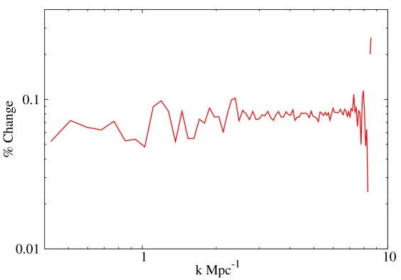
In the density field correlation function , two quantities change with redshift: 1) density fluctuations grow with time, 2) the mean density decreases because of the expansion of the Universe. Thus the evolving in principle would contribute to the light cone effect. In the linear regime the two quantities together scale as . For a distance of they jointly change along the LOS. We use very high redshift simulation cubes (before the reionization starts) and find enhancement in the 3D power spectrum on almost all scales (Figure 10). This result agrees with McQuinn et. al (2006) who predicted a constant enhancement in the power spectrum (see their Appendix A). The contribution of the evolving to the total light cone effect on the power spectrum is therefore negligible and hence we ignore this term in the rest of our analysis.
The evolution of is thus mainly dominated by the on scales larger or comparable to the size of ionized bubbles. For the rest of our analysis we only consider the term . The function which is defined as should be zero both for and . It also should satisfy the boundary conditions (for details see Zaldarriaga et al., 2004)
The correlation function can be calculated for a given bubble distribution as (Furlanetto et al., 2004)
| (12) | |||||
where is the volume of the overlap region between two ionized regions centered a distance apart. The function can be written as
In the next subsection we present some bubble size distributions measured from simulation. We will then model the bubble distribution and use that for the subsequent analysis.
4.2.1 Bubble size distribution and its evolution
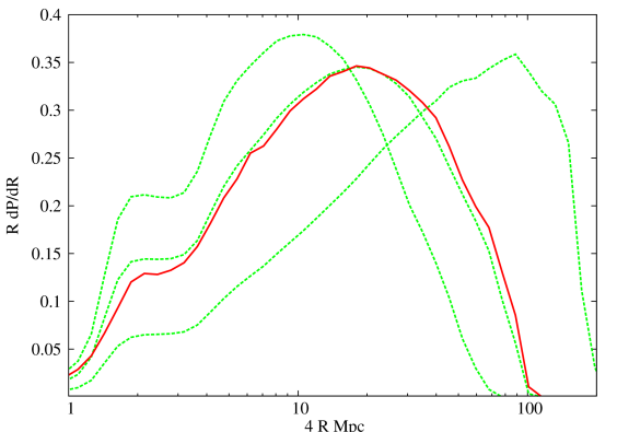
We calculate the bubble size distribution from the simulation using the spherical average method (see Friedrich et al., 2011, for more details on different bubble size estimates). Fig. 11 shows the bubble size distribution 666This is quantity is essentially same as and follows the condition for coeval cubes at three redshifts corresponding to the back, middle and front side of a light cone cube centered around redshift 9.09. It also shows the bubble size distribution in the light cone cube centered around 9.09. The coeval distributions at the three redshifts differ considerably. For example the radii at which the bubble distribution peaks are 10, 20, and 90 cMpc. Interestingly the bubble size distribution for the light cone cube is very similar to the coeval box at the central redshift. In the light cone cube the bubble size distribution would be the average of those of the coeval cubes in the redshift range where is the extent of the cube along redshift axis. Although the bubbles in the light cone cube are smaller/larger in the back/front side compared to the coeval cube, the average bubble distribution in the whole light cone cube is very similar to the coeval cube of the central redshift. Because of this ‘averaging effect’ the light cone effect is small even though there is a substantial evolution in the bubble distribution across the box.
We investigate further and to make the following calculations simpler we parameterize . This is motivated by Fig. 11 (see also Figure 2 in Furlanetto et al., 2004). We normalize the function using Eq. 8.
Now consider the case around the central redshift . Since the light cone cube covers the redshift range it will have slightly more bubbles both at the large and small bubble size ends than the coeval cube at redshift . This is exactly what we see in the simulation (Figs. 3 and 11).
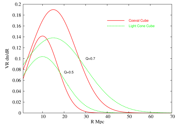
As we mentioned in Section 4.1 the average neutral fraction for a coeval cube at redshift and for a light cone cube centered around redshift is almost the same. We consider reionization for two values of and (see Eq. 8). Parameters for the bubble distribution are summarized in Table 3. Figure 12 shows the bubble distribution for (solid) and (dashed) for the coeval cube and the light cone cube. As we discussed above, there will be more large and small size bubbles in the light cone cube compared to the coeval cube, we approximate this by increasing for the light cone cube. The bubble size at which the quantity peaks has been kept same for both for a fixed . We also see in the Fig. 12 that for the number density of bubbles of size is higher in the light cone cube than the coeval cube. The ‘cross over radius’ i.e, the bubble radius beyond which the number density becomes higher than in the coeval cube is . For the cross over radius () is higher than for . This is because for higher the characteristic bubble size increases. Obviously, the exact distribution could be different but the general features such as the increase of characteristic bubble size and cross over radius for larger values, and larger bubbles in the light cone cube than the coeval cube, are likely to be true in all reionization scenarios where stars/QSOs are dominant sources. Since our aim is to qualitatively understand the effect of evolution, we can use these simplified distributions.
| Box | (cMpc) | (cMpc) | |
|---|---|---|---|
| coeval cube | 0.5 | ||
| Light cone cube | 0.5 | ||
| coeval cube | 0.7 | ||
| Light cone cube | 0.7 |
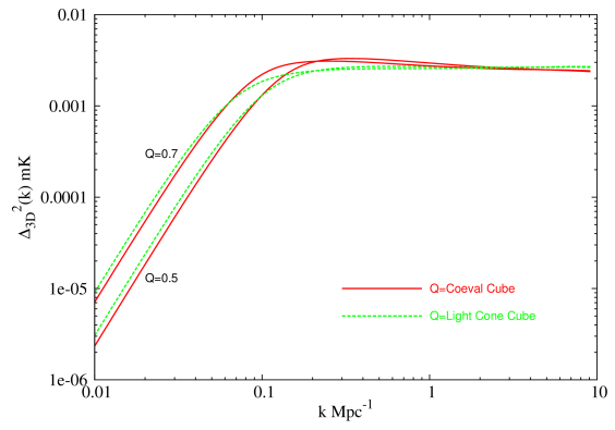
Figure 13 plots the power spectrum for the bubble distribution models we describe above. We see that there is a scale below () which the light cone cube has more power than the coeval cube and above () which it is the other way around. This is because the number of bubbles in the light cone cube below the cross-over radius is less than in the coeval cube. We call this scale the ‘cross-over mode’. We see this feature in Fig. 13 where the cross-over modes are and for and respectively. The cross-over mode is thus seen to shift towards larger scales (smaller ) as increases. This is because the cross-over radius is larger for . Based on these results we find the empirical relation between the cross-over radius and the cross-over mode to be
| (13) |
This simple toy model explains the two main features seen in the simulation results
-
1.
The power spectrum in the light cone cube is enhanced/suppressed on large/small scales compared to the one from the coeval cube at the central redshift.
-
2.
The cross-over mode shifts towards large scales as reionization proceeds.
As we pointed out in Sect. 3, we do not see a large effect when the mean ionization fraction is around , even though the evolution is across the light cone cube is substantial at that stage. We can now understand this to be because the cross-over mode shifts towards larger scales as reionization proceeds and around ionization the cross over scale is already almost the same as lowest mode that we can measure from our simulation volume, even though it has a size of 163 cMpc. We therefore predict that for a larger simulation volume, enhanced power on scales Mpc-1 will be found.
4.3 Taylor expansion of the power spectrum evolution
In addition to the more heuristic models given above, the following approach also helps in understanding some of the trends we see in Figure 4 and 5. We find that the coeval cube power spectrum for a given mode changes very smoothly with redshift . So we expand in a Taylor series around a central redshift as
| (14) |
where is the comoving distance from the central redshift to redshift and the parameters , , . We ignore the higher order terms. Next we calculate the light cone power spectrum by taking average of in the range around redshift using
| (15) |
where is the comoving LOS width. The above equation can be simplified to
| (16) |
We see that the linear term () and all terms with odd powers cancel out and only the quadratic term () and the other terms with even powers survive the averaging process. This supports our argument that the light cone effect is a ‘2nd order effect’ and that linear trends in the evolution of the power spectrum average out. The fractional change in the power spectrum due to the light cone effect is given by . Positive/negative values of the parameter denote that light cone power is suppressed/enhanced compared to the coeval value.
To test this quadratic approximation we use simulation L3 and fit the polynomial Eq. 14 for a given mode around three different central redshifts, taking . Using the values of we calculate the percentage change in the power spectrum and also measure the actual percentages from the simulation results. Values for three different modes are given in Table 4. From these it can be seen that the quadratic expansion correctly predicts the sign of the parameter and reproduces the trends seen in the simulations. During the early phases the match with the simulations is quite good, but at later stages it under predicts the changes. Most likely the discrepancies are due to the neglect of the higher order terms.
| (Mpc-1) | 0.081 | 0.167 | 1.02 | |||
|---|---|---|---|---|---|---|
| Q | S | Q | S | Q | S | |
| 21% | 52% | 16% | 24% | 4% | 12% | |
| -3.3% | -9% | 2.5% | 6% | 2.4% | 3% | |
| -24% | -30% | -11% | -10% | 0.6% | 1% | |
5 Effect of peculiar velocity on the light cone effect
The peculiar velocity of the IGM gas influences the 21-cm power spectrum (Bharadwaj et al., 2001; Bharadwaj & Ali, 2004). During the dark ages when the H I density is expected to trace the DM density, the spherical averaged power spectrum is enhanced by a factor of 1.87 at linear scales. As reionization proceeds, the relative contribution of the peculiar velocity to the 21-cm power spectrum changes considerably with redshift. For inside-out reionization scenario the peculiar velocity could increase the 21-cm power spectrum by a factor of (see Mao et al., 2011, Fig. 3) during a short period in the beginning of reionization (, see Mao et al., 2011, Fig. 3). When reionization is at its 50% phase, peculiar velocity effects slightly decreases the 21-cm power spectrum on the large scales relevant for the first generation of EOR experiments. In other words, peculiar velocity effects change the evolution of 21-cm power spectrum and hence could affect the light cone effect. We briefly investigate this here.
The method for taking the peculiar velocity into account when constructing the light cone cube was outlined in Mellema et al. (2006a) and described in detail in Mao et al. (2011); in the terminology of the latter we use the MM-RMM(1RT) scheme. The left panel of Figure 14 shows the 21-cm power spectrum with peculiar velocity for coeval cubes at three different redshifts (center and two ends) as well as for the light cone cube. The right panel shows the relative difference . The figure looks mostly very similar to Figure 4 where we did not include any peculiar velocity effects, the exception being the earliest stages, at redshift . Here the case with peculiar velocity shows a negligible light cone effect whereas the case for no peculiar velocity shows a difference in the power spectrum at large scales. The reason for this is that in the beginning of reionization bubble growth is relatively slow and evolution is dominated by the peculiar velocity. As reionization proceeds the evolution is mainly dominated by the growth of ionized bubbles and hence the peculiar velocity has almost no impact on the light cone effect. Note that this does not mean that the inclusion of peculiar velocity does not affect the power spectrum. In fact peculiar velocity causes comparable or even larger changes than the light cone effect. A more thorough exploration of the effects of peculiar velocity will be presented in future work.
6 Conclusions and discussion
We investigate the effect of evolution on the 3D and 1D LOS 21-cm power spectra during the entire period of reionization. We use three different EoR simulations in a volume of 163 cMpc on each side, one in which reionization is more gradual, ending at and two in which it is more rapid, ending at . In one of these rapid simulations, reionization is driven by more massive sources, leading to relatively larger ionized bubbles. Below we summarize our results:
-
•
For the cases we studied, the spherically averaged power spectrum changes up to in the range to using a redshift interval corresponding to the full extent of our simulation volume, . As expected, for smaller redshift bins the effect is found to be smaller. Large scales are affected more and the effects at smaller scales are minor.
-
•
Substantial evolution of the mean mass averaged neutral fraction , rms variations in the 21-cm signal, and bubble size distribution along the LOS axis are averaged out in the spherically averaged power spectrum. This averaging effect makes the light cone effect relatively small compared to the evolutionary changes along the LOS axis.
-
•
We can detect anisotropies in the the full 3D power spectra on large scales in the later stages of reionization, but are unable to quantify the -dependence of this effect with the simulations available to us.
-
•
The bubble size distribution in the light cone cube centered around redshifts is remarkably similar to the bubble size distribution in the coeval cube at , even if there is substantial evolution in the ionized fractions along the LOS. This is the reason why we see a relatively small effect on the 21-cm power spectrum compared to the amount of change in the and the rms of the 21-cm signal.
-
•
The large scale power is enhanced and the small scale power is suppressed most of the time except at the final phase of reionization where the power spectrum is suppressed at all scales we can measure in our simulations. In other words, there is a ‘cross-over mode’ below and above which the power is enhanced and suppressed respectively. The cross-over mode shifts towards lower -mode (large scale) as reionization proceeds.
-
•
Surprisingly we see very little effect when reionization is complete and there is a rapid evolution in the and the rms. We argue that at this stage of reionization the cross-over mode is already comparable to the lowest mode we can measure from the simulation and enhancement of power should be present at larger scales than that.
-
•
Despite the fact that the reionization histories differ considerably between the three simulations, we see quite similar results.
-
•
Growth of structures with redshift and the expanding background enhance the power spectrum by for our cMpc cube. Its evolution is therefore dominated by the ionization field during the reionization.
-
•
An analytical toy model (Toy model 1) can explain the large scale power enhancement due to light cone effect as well as its smallness.
-
•
A second analytical toy model (Toy model 2) for a light cone cube with more large bubbles beyond some cross-over radius and less bubbles below that, can explain all the features we see in the simulation results.
-
•
The presence of more large bubbles and fewer small bubbles of size is responsible for the enhanced/suppressed power on scales below/above . The fact that the cross-over scale shifts towards lower as reionization proceeds is because the cross-over bubble size increases as reionization proceeds.
-
•
Interestingly we find that the light cone effect is less prominent in the 1D LOS power spectra.
We should note that instruments such as LOFAR and MWA are expected to measure down to Mpc-1, scales larger than we were able to analyze here (). From our results we expect enhanced power on those scales in the light cone cube. Especially when reionization is around we expect more enhanced power on these larger scales. Reionization simulations of even larger cosmological volumes would be useful to better understand the effects at those scales. On the other hand, the aforementioned telescopes will not reach beyond Mpc-1 making the small scale light cone effects observationally less relevant.
The removal of the large foreground signals of the EoR 21cm signal is expected to affect the large scale LOS modes significantly. Although details about which scales will be affected depend on the subtraction technique used, it is obvious that if is the comoving length over which the foreground subtraction is performed, modes with cannot be extracted (McQuinn et. al, 2006). The equivalent bandwidth for the simulation boxes we consider is and it is likely that foreground subtraction techniques will use considerably larger bandwidths (see e.g, Chapman et al., 2012). The same authors also show that foreground residuals do not affect the extraction of the 3D spherically averaged power spectrum over bandwidths of 8 MHz. However, the effects of foregrounds remain clearly an issue which requires careful consideration when considering LOS effects in the 21cm signal.
In our simulations the spherically averaged power spectra are based on equal numbers of modes in the LOS and transverse directions. However, most of the ongoing and upcoming surveys will not sample the full range in the spatial and frequency directions for many -modes. This is due to the fact that they have better resolution in the frequency (LOS) direction than in the spatial directions. For example the LOFAR core has a maximum baseline which corresponds a maximum transverse mode . The intrinsic frequency resolution of the array is better than 1 kHz, but likely the observed data will be stored with frequency resolution, equivalent to LOS mode . When using this resolution to calculate the spherically averaged power spectra, the LOS modes will contribute more compared to the transverse modes for . Since the light cone effect makes the power spectra anisotropic i.e, different power for different combintions of for a given , the lack of small scale transverse modes , in principle, would affect the power spectra measurements at those -modes. However, as shown in Fig. 7, small scales are hardly anisotropic due to the light cone effect so we do not expect those modes to be affected much due to the incomplete sampling of small scale modes. In addition, small scales are expected to be dominated by system noise and are unlikely to be measured.
Based on our results, we conclude that the light cone effect is important especially at scales where the first generation of low frequency instruments are sensitive. It can bias cosmological and astrophysical interpretations unless this effect is understood and incorporated properly.
Acknowledgment
We would like to thank the anonymous referee for his constructive comments which have helped to improve the paper. Discussions with Saleem Zaroubi and other members of the LOFAR EoR Key Science Project have been valuable for the work described in this paper. KKD is grateful for financial support from Swedish Research Council (VR) through the Oscar Klein Centre (grant 2007-8709). The work of GM is supported by the Swedish Research Council grant 2009-4088. The authors acknowledge the Texas Advanced Computing Center (TACC) at The University of Texas at Austin for providing HPC resources, under NSF TeraGrid grants TG-AST0900005 and TG-080028N and TACC internal allocation grant “A-asoz”, as well as the Swedish National Infrastructure for Computing (SNIC) resources at HPC2N (Umeå, Sweden), which have contributed to the research results reported in this paper. This work was supported in part by NSF grants AST-0708176 and AST-1009799, NASA grants NNX07AH09G, NNG04G177G and NNX11AE09G, and Chandra grant SAO TM8-9009X. ITI was supported by The Southeast Physics Network (SEPNet) and the Science and Technology Facilities Council grants ST/F002858/1 and ST/I000976/1. KA is supported in part by Basic Science Research Program through the National Research Foundation of Korea (NRF) funded by the Ministry of Education, Science and Technology (MEST; 2009-0068141,2009-0076868).
References
- Ali et al. (2005) Ali, S. S., Bharadwaj, S., & Pandey, B. 2005, MNRAS, 363, 251
- Ali et al. (2008) Ali, S. S., Bharadwaj, S., & Chengalur, J. N. 2008, MNRAS, 385, 2166
- Alvarez et al. (2009) Alvarez, M. A., Busha, M., Abel, T., & Wechsler, R. H. 2009, ApJL, 703, L167
- Baek et al. (2009) Baek, S., Di Matteo, P., Semelin, B., Combes, F., & Revaz, Y. 2009, A & A, 495, 389
- Baek et al. (2010) Baek, S., Semelin, B., Di Matteo, P., Revaz, Y., & Combes, F. 2010, A & A, 523, A4
- Barkana & Loeb (2005) Barkana, R., & Loeb, A. 2005, ApJL, 624, L65
- Barkana & Loeb (2006) Barkana, R., & Loeb, A. 2006, MNRAS, 372, L43
- Barkana (2009) Barkana, R. 2009, MNRAS, 397, 1454
- Becker et al. (2001) Becker, R. H., et al. 2001, AJ, 122, 2850
- Bernardi et al. (2009) Bernardi, G., et al. 2009, Astronomy & Astrophysics, 500, 965
- Bharadwaj et al. (2001) Bharadwaj, S., Nath, B. B., & Sethi, S. K. 2001, Journal of Astrophysics and Astronomy, 22, 21
- Bharadwaj & Ali (2004) Bharadwaj, S., & Ali, S. S. 2004, MNRAS, 352, 142
- Bowman & Rogers (2010) Bowman, J. D., & Rogers, A. E. E. 2010, Nature, 468, 796
- Chapman et al. (2012) Chapman, E., Abdalla, F. B., Harker, G., Jelić, V., Labropoulos, P., Zarubi, S., Brentjens, M. A., de Bruyn, A. G., & Koopmans, L. V. E. 2012, arXiv:1201.2190
- Chen & Miralda-Escudé (2004) Chen, X., & Miralda-Escudé, J. 2004, ApJ, 602, 1
- Choudhury et al. (2009) Choudhury, T. R., Haehnelt, M. G., & Regan, J. 2009, MNRAS, 394, 960
- Chuzhoy & Shapiro (2006) Chuzhoy, L., & Shapiro, P. R. 2006, ApJ, 651, 1
- Datta et al. (2007) Datta, K. K., Choudhury, T. R., & Bharadwaj, S. 2007, MNRAS, 378, 119
- Fan et al. (2006) Fan, X., et al. 2006, AJ, 132, 117
- Fan et al. (2006a) Fan, X., Carilli, C. L., & Keating, B. 2006a, Annual Review of Astronomy & Astrophysics, 44, 415
- Field (1959) Field, G. B. 1959, ApJ, 129, 536
- Friedrich et al. (2011) Friedrich, M. M., Mellema, G., Alvarez, M. A., Shapiro, P. R., & Iliev, I. T. 2011, MNRAS, 413, 1353
- Furlanetto et al. (2004) Furlanetto, S. R., Zaldarriaga, M., & Hernquist, L. 2004, ApJ, 613, 1
- Furlanetto et al. (2006) Furlanetto, S. R., Oh, S. P., & Briggs, F. H. 2006, Physics Reports, 433, 181
- Geil & Wyithe (2008) Geil, P. M., & Wyithe, J. S. B. 2008, MNRAS, 386, 1683
- Harker et al. (2010) Harker, G., et al. 2010, MNRAS, 405, 2492
- Hirata (2006) Hirata, C. M. 2006, MNRAS, 367, 259
- Iliev et al. (2006) Iliev, I. T., Mellema, G., Pen, U.-L., Merz, H., Shapiro, P. R., & Alvarez, M. A. 2006, MNRAS, 369, 1625
- Iliev et al. (2007) Iliev, I. T., Mellema, G., Shapiro, P. R., & Pen, U.-L. 2007, MNRAS, 376, 534
- Iliev et al. (2008) Iliev, I. T., Mellema, G., Pen, U.-L., Bond, J. R., & Shapiro, P. R. 2008, MNRAS, 384, 863
- Iliev et al. (2011) Iliev, I. T., Mellema, G., Shapiro, P. R., Pen, U.-L., Mao, Y., Koda, J., & Ahn, K. 2011, arXiv:1107.4772
- Kashikawa et al. (2011) Kashikawa, N., et al. 2011, arXiv:1104.2330
- Komatsu et al. (2011) Komatsu, E., et al. 2011, ApJS, 192, 18
- Larson et al. (2011) Larson, D., et al. 2011, ApJS, 192, 16
- Lidz et al. (2008) Lidz, A., Zahn, O., McQuinn, M., Zaldarriaga, M., & Hernquist, L. 2008, ApJ, 680, 962
- Lonsdale et al. (2009) Lonsdale, C. J., et al. 2009, IEEE Proceedings, 97, 1497
- Majumdar et al. (2010) Majumdar, S., Bharadwaj, S., Datta, K. K., & Choudhury, T. R. 2011, MNRAS, 413, 1409
- Mao et al. (2011) Mao, Y., Shapiro, P. R., Mellema, G., Iliev, I. T., Koda, J., & Ahn, K. 2011, arXiv:1104.2094
- Malhotra & Rhoads (2004) Malhotra, S., & Rhoads, J. E. 2004, ApJL, 617, L5
- Matsubara et al. (1997) Matsubara, T., Suto, Y., Szapudi, I. 1997, ApJL, 491, L1
- McQuinn et. al (2006) McQuinn, M., Zahn, O., Zaldarriaga, M., Hernquist, L., & Furlanetto, S. R. 2006, ApJ, 653, 815
- McQuinn et al. (2007) McQuinn, M., Lidz, A., Zahn, O., Dutta, S., Hernquist, L., & Zaldarriaga, M. 2007, MNRAS, 377, 1043
- Mellema et al. (2006a) Mellema, G., Iliev, I. T., Pen, U.-L., & Shapiro, P. R. 2006a, MNRAS, 372, 679
- Mellema et al. (2006b) Mellema, G., Iliev, I. T., Alvarez, M. A., & Shapiro, P. R. 2006b, New Astronomy, 11, 374
- Mesinger & Furlanetto (2007) Mesinger, A., & Furlanetto, S. 2007, ApJ, 669, 663
- Mitra et al. (2011) Mitra, S., Choudhury, T. R., & Ferrara, A. 2011, MNRAS, 413, 1569
- Morales & Wyithe (2010) Morales, M. F., & Wyithe, J. S. B. 2010, Annual Review of Astronomy and Astrophysics, 48, 127
- Ouchi et al. (2010) Ouchi, M., et al. 2010, ApJ, 723, 869
- Paciga et al. (2010) Paciga, G., et al. 2010, MNRAS(accepted), arXiv:1006.1351
- Parsons et al. (2010) Parsons, A. R., et al. 2010, AJ, 139, 1468
- Peacock (1999) Peacock, J. A. 1999, Cosmological Physics, Cambridge University Press, pp. 498
- Pen et al. (2009) Pen, U.-L., Chang, T.-C., Hirata, C. M., Peterson, J. B., Roy, J., Gupta, Y., Odegova, J., & Sigurdson, K. 2009, MNRAS, 399, 181
- Purcell & Field (1956) Purcell, E. M., & Field, G. B. 1956, ApJ, 124, 542
- Santos et al. (2008) Santos, M. G., Amblard, A., Pritchard, J., Trac, H., Cen, R., & Cooray, A. 2008, ApJ, 689, 1
- Santos et al. (2010) Santos, M. G., Ferramacho, L., Silva, M. B., Amblard, A., & Cooray, A. 2010, MNRAS, 406, 2421
- Sethi (2005) Sethi, S. K. 2005, MNRAS, 363, 818
- Sethi & Haiman (2008) Sethi, S., & Haiman, Z. 2008, ApJ, 673, 1
- Shapiro et al. (2006) Shapiro, P. R., Iliev, I. T., Alvarez, M. A., & Scannapieco, E. 2006, ApJ, 648, 922
- Shin et al. (2008) Shin, M.-S., Trac, H., & Cen, R. 2008, ApJ, 681, 756
- Thomas et al. (2009) Thomas, R. M., et al. 2009, MNRAS, 393, 32
- Thomas & Zaroubi (2011) Thomas, R. M., & Zaroubi, S. 2011, MNRAS, 410, 1377
- Totani et al. (2006) Totani, T., Kawai, N., Kosugi, G., Aoki, K., Yamada, T., Iye, M., Ohta, K., & Hattori, T. 2006, Publications of the Astronomical Society of Japan, 58, 485
- Trac & Gnedin (2009) Trac, H., & Gnedin, N. Y. 2009, arXiv:0906.4348
- Willott et al. (2009) Willott, C. J., et al. 2009, AJ, 137, 3541
- Wouthuysen (1952) Wouthuysen, S. A. 1952, AJ, 57, 31
- Wyithe et al. (2005) Wyithe, J. S. B., Loeb, A., & Barnes, D. G. 2005, ApJ, 634, 715
- Yu (2005) Yu, Q. 2005, ApJ, 623, 683
- Zahn et al. (2007) Zahn, O., Lidz, A., McQuinn, M., Dutta, S., Hernquist, L., Zaldarriaga, M., & Furlanetto, S. R. 2007, ApJ, 654, 12
- Zaldarriaga et al. (2004) Zaldarriaga, M., Furlanetto, S. R., & Hernquist, L. 2004, ApJ, 608, 622
- Zygelman (2005) Zygelman, B. 2005, ApJ, 622, 1356
Appendix A Effect of inclusion of modes on the power spectrum
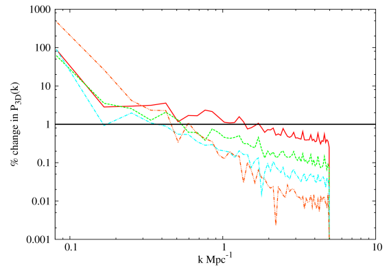
Radio interferometric experiments cannot measure the modes at where , are two components of the baseline vector and is the comoving distance. In order to predict the expected 21-cm power spectra for some reionization model or interpret the observed 21-cm power spectra the modes should be excluded when the power spectrum is calculated from the simulated data. Figure 15 plots with for different redshifts for light cone cubes. Here and are the 3D power spectra including and excluding the modes respectively. We find that power is enhanced by for Mpc-1. The reason is that for the light cone cube there is a gradual change in the mean brightness with redshift. Large scale LOS modes with gain power because of this and hence affect the large modes in the spherically averaged power spectrum. We find that the coeval cubes are hardly affected because the mean is similar for all slices. We also note that for the simulations studied in this paper, exclusion of the modes is practically the same as the subtraction of the mean brightness temperature from each single frequency 21-cm map.