Symmetry breaking between statistically equivalent, independent channels in a few-channel chaotic scattering

Abstract

We study the distribution function $P(\omega)$ of the random variable $\omega=\tau_{1}/(\tau_{1}+\ldots+\tau_{N})$, where $\tau_{k}$’s are the partial Wigner delay times for chaotic scattering in a disordered system with $N$ independent, statistically equivalent channels. In this case, $\tau_{k}$’s are i.i.d. random variables with a distribution $\Psi(\tau)$ characterized by a ”fat” power-law intermediate tail $\sim 1/\tau^{1+\mu}$, truncated by an exponential (or a log-normal) function of $\tau$. For $N=2$ and $N=3$, we observe a surprisingly rich behavior of $P(\omega)$ revealing a breakdown of the symmetry between identical independent channels. For $N=2$, numerical simulations of the quasi one-dimensional Anderson model confirm our findings.

Scattering by chaotic or disordered systems is encountered in various situations ranging from nuclear, atomic or molecular physics to mesoscopic devices yan1 . The key property characterizing the scattering process is the unitary $S$ matrix relating the amplitudes of waves incoming to the system and those of scattered waves. Since the underlying dynamics is chaotic, the properties of the $S$ matrix behave in an irregular way when the parameters of the incoming waves or of the medium are modified. Hence, an adequate description of the scattering process requires the knowledge of the $S$ matrix distribution.

Time-dependent aspects of the scattering process are well captured by the Wigner delay time (WDT) $\tau$ wigner , defined through the derivative of the $S$ matrix with respect to energy $E$. Physically, $\tau$ is an excess time spent in the interaction region by a wave packet with energy peaked at $E$, as compared to a free wave packet propagation.

For systems coupled to the outside world via $N$ open channels, $\tau=\sum_{k=1}^{N}\tau_{k}$, where $\tau_{k}=\partial\theta_{k}/\partial E$ are the partial delay times and $\theta_{k}$ are the phase shifts of the $S$ matrix. One shows that $\tau_{k}$’s are the diagonal elements of the Wigner-Smith time delay matrix (WSM), taken in the eigenbasis of the scattering matrix corr . Note that it is also customary to define the eigenvalues of the WSM as the proper delay times $\tau_{k}^{\prime}$ (see, e.g., Ref. yan1 ; beenaker ). Beyond the $1$-channel case, $\tau_{k}$ and $\tau_{k}^{\prime}$ differ, although their sums over all scattering channels are equal to each other.

Likewise the $S$-matrix, the WDT is a random variable, whose distribution $\Psi(\tau)$ has a generic form comtet2 ; bolton ; ossipov ; steinbach ; geisel ; fyod ; fJLett ; sym ; 2 ; 3 ; corr :

$$\Psi(\tau)=\frac{a^{\mu}}{\Gamma(\mu)}\exp\left(-\frac{a}{\tau}\right)\,\frac{1}{\tau^{1+\mu}}\,,$$ (1)

where $a$ is a characteristic parameter, $\Gamma(\mu)$ is the gamma function and $\mu$ is a model-dependent exponent: one encounters situations with $0<\mu<1$, $\mu=1$ and $\mu>1$.

For 1D single-channel systems with weak disorder $\mu=1$ comtet2 ; bolton ; ossipov , which holds also for quasi-1D disordered systems of length $L\gg\lambda$, where $\lambda$ is the localization length fJLett . One can demonstrate the validity of this result for a single-channel scattering in any dimension in the regime of strong localization 3 . In 1D quasi-periodic systems with a single open channel and fractal dimension $D_{0}^{E}$ ($\leq 0.5$) of the spectrum one has $\mu=1-D_{0}^{E}<1$ steinbach , and $\mu=1/2$ holds for the 2D generalization of a kicked rotor model fyod ; geisel , as well as for generic weakly open chaotic systems in a parametrically large range of delay times yan1 ; fyod . Lastly, $\mu=1+N\beta/2>1$, where $\beta$ is the Dyson symmetry index, was obtained for ballistic scattering from a cavity sym ; 2 ; 3 .

It is however clear that Eq. (1) defines a limiting form, valid either for $L\to\infty$ or for weakly open systems. In reality, the power-law tail is truncated, such that all moments of $\Psi(\tau)$ exist. Two model-dependent cut-offs seem to be physically plausible (although not exact) comtet2 :

$$\Psi_{1}(\tau)=\frac{1}{2}\frac{\left(ab\right)^{\mu/2}}{K_{\mu}(2\sqrt{a/b})}\exp\left(-\frac{a}{\tau}\right)\,\frac{1}{\tau^{1+\mu}}\exp\left(-\frac{\tau}{b}\right)\;,$$ (2)

$K_{\mu}(x)$ being the modified Bessel function, and a log-normally truncated (LNT) form with $\exp(-\ln^{2}(\tau)/c)$ in place of $\exp(-\tau/b)$, where $b$ and $c$ are either $\sim L$ yan1 ; comtet2 , or to the opening degree for weakly open systems yan1 ; fyod .

In this paper we are concerned with a somewhat unusual statistics of partial delay times for scattering in systems with $N$ equivalent channels. We focus here on

$$\omega=\frac{\tau_{1}}{\tau_{1}+\tau_{2}+...+\tau_{N}},$$ (3)

a random variable which probes the contribution of one of the channels to the WDT and hence, the symmetry between different channels. To highlight the effect of the intermediate power-law tail of $\Psi(\tau)$, we suppose that the channels are independent of each other such that the partial delay times $\tau_{k}$’s are i.i.d. random variables with a common distribution in Eqs. (1) or (2) (or a LNT form). This situation can be realized experimentally, e.g., for scattering in a bunch of disordered fibers. Such a simplified model with $\mu=1$ is also appropriate for a multichannel scattering from a piece of strongly disordered media when the distance between the scattering channels locations exceeds $\lambda$. The role of correlations will be briefly discussed at the end of this paper.

We show here, on example of $2$- and $3$-channel systems, that intermediate power-law tails entail a surprisingly rich behavior of the distribution

$$P(\omega)=\left<\delta\left(\omega-{\tau_{1}}/{(\tau_{1}+\tau_{2}+...+\tau_{N})}\right)\right>,$$ (4)

where $\langle\dots\rangle$ denotes an average over the distributions of $\tau_{k}$’s. We realize that $\omega$ exhibits significant sample-to-sample fluctuations and, in general, the symmetry between identical independent channels is broken, despite the fact that all the moments of $\Psi(\tau)$ are well defined. A similar result was found for related mathematical objects in Refs. redner ; we_jstat . We address the reader to Ref. we_jstat for the details on the derivation of $P(\omega)$.

For $N=2$ and $\Psi(\tau)$ as in Eq. (1), we get:

$$P(\omega)\equiv B\,\omega^{\mu-1}\left(1-\omega\right)^{\mu-1}.$$ (5)

with $B={\Gamma(2\mu)}/{\Gamma^{2}(\mu)}$.

Figure 1: (Color online) $N=2$. $P(\omega)$ in Eq. (5) for different values of $\mu$. The dashed line depicts $P(\omega)$, Eq. (9), with $\beta=2$ $(\mu=4)$.

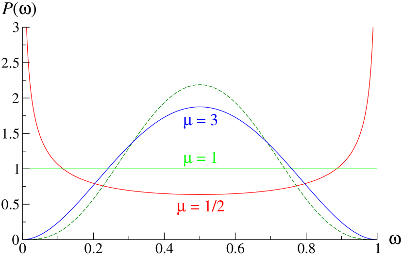
A striking feature of the beta-distribution in Eq. (5) is that its very shape depends on whether $0<\mu<1$, $\mu=1$ or $\mu>1$ (see Fig. 1). For $0<\mu<1$, $P(\omega)$ is bimodal with a $U$-like shape, and most probable values being $0$ and $1$. In this case, the symmetry between two identical independent channels is broken and either of the two channels provides a dominant contribution to the WDT. Strikingly, $\langle\omega\rangle=1/2$ corresponds here to the least probable value of $\omega$. For $\mu=1$, $P(\omega)\equiv 1$, and either of the channels may provide any contribution to the overall delay time with equal probability. Finally, for $\mu>1$, $P(\omega)$ is unimodal, which signifies that both channels contribute proportionally.

For $N=2$ and a truncated $\Psi(\tau)$ as in Eq. (2) we get

$$P(\omega)=B[\omega(1-\omega)]^{-1}{K_{2\mu}\left(2\sqrt{a/b\,\omega(1-\omega)}\right)}\,.$$ (6)

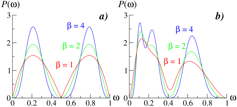
where $B=[{2K_{\mu}^{2}(2\sqrt{a/b})}]^{-1}$. Note that $P(\omega)$ vanishes at the edges and is symmetric around $\omega=1/2$. The behavior of $P(\omega)$ can be analyzed by expanding the expression in Eq. (6) in Taylor series at $\omega=1/2$ we_jstat . For $\mu>1$, $P(\omega)$ is a bell-shaped function with a maximum at $\omega=1/2$. For $\mu=1$, for which we previously found a uniform distribution, the latter (apart from an exponential cut-off at the edges) is approached in the limit $b/a\gg 1$ [see Fig.2 a)].

Figure 2: (Color online) $P(\omega)$ for $N=2$ and $\Psi(\tau)$ in Eq. (2) with $a=1$. a): for $\mu=1$ and different $b$. b): for $\mu=1/2$ and different $b$.

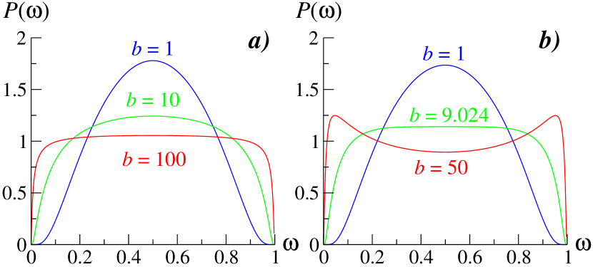
For $0<\mu<1$ the situation is more complicated: there exists a critical value $b_{c}$ separating two different regimes. For $b<b_{c}$, $P(\omega)$ is a bell-shaped function with a maximum at $\omega=1/2$. For $b=b_{c}$, $P(\omega)\approx 1$ except for narrow regions at the edges, where it vanishes exponentially. Finally, for $b>b_{c}$ $P(\omega)$ has an $M$-like shape, with maxima close to $\omega=0$ and $\omega=1$, $\omega=1/2$ being the least probable value. Hence, an exponential truncation of $\Psi(\tau)$ does not restore the symmetry between different channels, which holds only for systems whose size is less than some critical length set by $b_{c}$. Note that for a LNT form the overall behavior of $P(\omega)$ is very similar and also exhibits a transition at some value of the parameter $c$.

Further on, for $N=3$ and $\Psi(\tau)$ as in (1),

$$P(\omega)=C\frac{\left(1-\omega\right)^{\mu-1}}{\omega^{1+\mu}}\,_{2}F_{1}\left(2\mu,3\mu;2\mu+\frac{1}{2};\frac{\omega-1}{4\omega}\right)$$ (7)

where $C=\frac{\sqrt{\pi}}{2^{4\mu-1}}\;\frac{\Gamma(2\mu)\Gamma(3\mu)}{\Gamma^{3}(\mu)\Gamma(2\mu+1/2)}$ and ${}_{2}F_{1}$ is a hypergeometric series. One finds from Eq. (7) that $P(\omega)\sim(1-\omega)^{\mu-1}$ when $\omega\to 1$ and $P(\omega)\sim\omega^{\mu-1}$ when $\omega\to 0$, which agrees with the result in Eq. (5). On the other hand, the amplitudes in these asymptotic forms appear to be very different such that $P(\omega)$ is skewed to the left [see Fig. 3 a)].

Figure 3: (Color online) $N=3$. a): $P(\omega)$ in Eq. (7) for different values of $\mu$. b): $P(\omega)$ in Eq. (8) for $\mu=1/2$ and for different values of $b$ ($a$ is set equal to $1$).

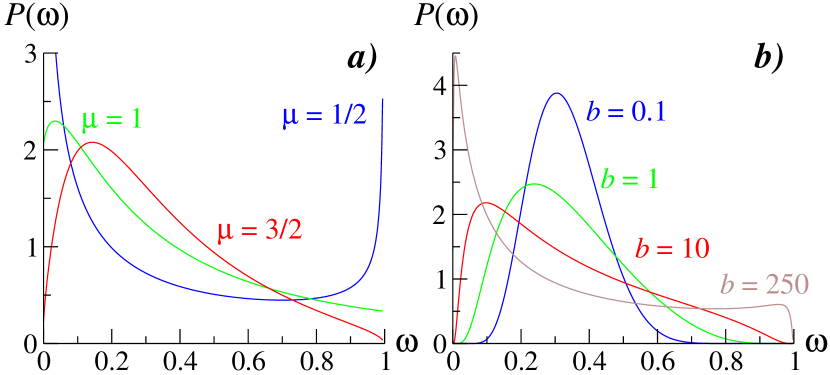
Therefore, for $N=3$, $P(\omega)$ diverges at both edges and has a $U$-shaped form for $0<\mu<1$ (see Fig. 3  a), which signifies that the symmetry between the channels is broken. For $\mu\geq 1$ the distribution is unimodal. Remarkably, for $\mu\geq 1$ the maximum $\omega_{m}$ of $P(\omega)$ is not at $\omega=1/3$: for $\mu=3$, one has $\omega_{m}=0.2719$, for $\mu=10$ the maximum is at $\omega_{m}=0.3102$ and etc; actually, $\omega_{m}\to 1/3$ only when $\mu\to\infty$. This means that even for $\mu>1$, $\omega$ exhibits sample to sample fluctuations and the average value $\langle\omega\rangle\equiv 1/3$ does not have any significance.

For $N=3$ and a truncated $\Psi(\tau)$ as in Eq. (2) we get

$$P(\omega) = \frac{(b/4a)^{3\mu/2}}{2K^{3}_{\mu}\left(2\sqrt{a/b}\right)}\frac{\omega^{\mu-1}}{(1-\omega)^{\mu+1}}\int^{\infty}_{0}dx\,x^{\mu}\,J_{\mu-1}\left(x\right)$$ (8)

$$\times \left(x^{2}+\frac{4a}{b\omega}\right)^{\mu}\,K^{2}_{\mu}\left(\sqrt{\frac{\omega}{1-\omega}\left(x^{2}+\frac{4a}{b\omega}\right)}\right),$$

where $J_{\mu}(x)$ is the Bessel function. We observe that $P(\omega)$ in Eq. (8) is always a bell-shaped function for $\mu\geq 1$. The most probable value $\omega_{m}$ is, however, always substantially less than $1/3$, approaching this value only when $\mu\to\infty$ or $b\to 0$. The case $0<\mu<1$ is different: For $b/a\ll 1$, $P(\omega)$ is peaked at $\omega_{m}\approx 1/3$. For larger $b/a$, $\omega_{m}$ moves towards the origin and $P(\omega_{m})$ decreases. For yet larger $b/a$, $\omega_{m}$ keeps moving towards the origin but now $P(\omega_{m})$ passes through a minimum and then starts to grow. At some special value of $b/a$ ($b/a\approx 140$ for $\mu=1/2$) a second extremum emerges (at $\omega\approx 0.84$ for $\mu=1/2$) which then splits into a minimum and a maximum and $P(\omega)$ becomes bimodal. For still larger $b/a$, the minimum moves towards $\omega=1/2$, while the second maximum moves to $\omega=1$. For $N=3$ and a LNT form of $\Psi(\tau)$, we observe essentially the same behavior.

To substantiate our theoretical predictions, we performed a numerical analysis of $\Psi(\tau)$ and $P(\omega)$ for a quasi 1D disordered Anderson model defined on a rectangular lattice of size $L\times W$ (with $L=100$ and $W=3$) with two single-channel leads connected to sites $(1,2)$ and $(L,2)$. Our (isolated) system is described by the Hamiltonian $H=\sum_{i}\epsilon_{i}{|i\rangle}{\langle i|}+\sum_{i\neq j}t_{ij}{|i\rangle}{\langle j|}$, where $t_{ij}$ are the hopping rates between the neighboring sites $i$ and $j$, and $\epsilon_{i}$ is the energy at the site $i$, which is a centered, $\delta$-correlated Gaussian random variable.

Our numerical results are summarized in Fig. 4. In the left panel we depict $\Psi(\tau)$ for different values of the localization length $\lambda\sim 1/\langle\epsilon_{i}^{2}\rangle$. For $\lambda/L\ll 1$, one observes that $\Psi(\tau)$ decays asymptotically as $1/\tau^{2}$, which corresponds to $\mu=1$. On the other hand, $\Psi(\tau)$ clearly exhibits an intermediate regime with a slower than $1/\tau^{2}$ decay $(\mu<1)$. When $\lambda$ increases, this intermediate regime shrinks and also the asymptotic decay becomes faster (possibly, a log-normal).

Figure 4: (Color online) Distributions $\Psi(\tau)$ and $P(\omega)$ for a quasi-1D Anderson wire for different values of $\lambda$: from top to bottom $\lambda=3$, $100$ and $200$. In the left panel we plot $\tau^{-2}$ (dashed green curve) and $\tau^{-1}$ (solid blue curve). In the right panel the dashed red curve is the corresponding $P(\omega)$ calculated under the assumption of statistical independence of the $\tau_{k}$s.

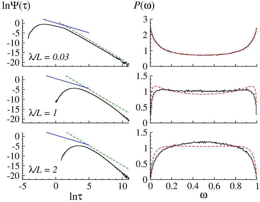
The right panel shows the corresponding distributions $P(\omega)$, evidencing a transition from $U$-like to bell-shaped curves upon an increase of disorder. The $U$-like shape ($\lambda/L\ll 1$, top right) stems out of the intermediate regime with $\mu<1$. Interestingly, the critical distribution $P(\omega)\approx 1$ is observed for $\lambda/L\simeq 1$ (middle right), i.e., when $\lambda$ is equal to the length of the system. For $\lambda/L>1$, a faster than $1/\tau^{2}$ decay of $\Psi(\tau)$ leads to a bell-shaped $P(\omega)$.

As a test of statistical independence of the actual $\tau_{k}$’s, we have computed the distribution $P_{uncor}(\omega)$ (dashed red curves in Fig. 4) of the random variable $\tau_{1}/(\tau_{1}+\tau_{2})$ where $\tau_{1}$ and $\tau_{2}$ are i.i.d. random variables drawn from the numerically observed $\Psi(\tau)$. One notices a good agreement between $P(\omega)$ (black histogram) and $P_{uncor}(\omega)$, which is a clear indication of the lack of correlations between the different channels for $\lambda/L\ll 1$. Correlations between channels induce some discrepancies between $P(\omega)$ and $P_{uncor}(\omega)$ only for $\lambda/L\gtrsim 1$, when the extension of the typical eigenfunction becomes of the order of the system size. Consequently, the scattering exhibits a transition as the strength of the disorder is varied: $\tau_{1}$ and $\tau_{2}$ are most likely very different for $\lambda/L<1$ and most likely the same for $\lambda/L>1$. We conjecture that our findings can be extrapolated to thin 3D disordered wires, leading to a disproportionate contribution of the open channels to the total scattering in the diffusive regime, and a proportionate contribution in the metallic regime.

Figure 5: (Color online) $P(\omega)$ for the proper delay times for different values of $\beta$. a): $N=2$, Eq. (10). b): $N=3$.

To summarize, we have studied the distribution $P(\omega)$ of the random variable $\omega$, Eq. (3), which defines the contribution of a given channel to the WDT in a system with a few open, independent, statistically equivalent channels. We have shown that for $2$-channel systems intermediate power-law tails with $\mu\leq 1$ in the distribution of the partial delay times entail breaking of the symmetry between the channels; $P(\omega)$ has a characteristic $U$-shape form and the average $\langle\omega\rangle=1/2$ corresponds to the least probable value. For $\mu>1$ the symmetry is statistically preserved and $\langle\omega\rangle=1/2$ is also the most probable value. For $N=3$ the symmetry between the channels is always broken which results in unusual bimodal forms of $P(\omega)$.

Finally, we briefly comment on the effect of correlations on $P(\omega)$. We mention two known results on the joint distributions of the partial and of the proper delay times for which we can evaluate $P(\omega)$ exactly. The joint distribution function of any two partial delay times in a system with $N$ channels and arbitrary $\beta$ has been calculated in Ref. corr . From this result, we compute exactly the distribution $P(\omega)$ for two statistically equivalent (but not independent) channels:

$$P(\omega)=D\,\omega^{3\beta/2}\left(1-\omega\right)^{3\beta/2}\,,$$ (9)

with $D=\frac{\Gamma(2+3\beta)}{\Gamma^{2}(1+3\beta/2)}$, which is also a beta-distribution, but with an exponent ($=3\beta/2$) larger than the one ($=\beta/2$) in Eq. (5) corresponding to two independent channels. For the same $\beta$, the distribution in Eq. (9) is narrower than $P(\omega)$ in Eq. (5) with $\mu=1+\beta/2$ (see Fig. 1). Hence, one may argue that the partial delay times attract each other, which interaction competes with the symmetry breaking produced by the intermediate power-law tails. Note, as well, that the larger $\beta$ is, the narrower is the distribution $P(\omega)$.

The joint distribution of $N$ proper delay times in a system with $N$ open channels is also known exactly beenaker . It turns out to be given by the Laguerre ensemble of random-matrix theory and is defined as a product of $\prod_{k=1}^{N}\Psi(\tau^{\prime}_{k})$, where each $\Psi(\tau_{k}^{\prime})$ as in (1) with $\mu=1+N\beta/2$, times the Dyson’s circular ensemble, $\prod_{i<j}|1/\tau_{i}^{\prime}-1/\tau_{j}^{\prime}|^{\beta}$. Due to the latter factor, the $\tau_{k}^{\prime}$s harshly repel each other. For $N=2$, we obtain

$$P(\omega)=F\,\omega^{\beta}(1-\omega)^{\beta}|1-2\omega|^{\beta},$$ (10)

where $F$ is a computable normalization constant. Remarkably, $P(\omega)$ in (10) is a product of the beta-distribution in Eq. (5) and a factor $|1-2\omega|^{\beta}$, which is a new feature here and stems from the correlations between $\tau_{1}^{\prime}$ and $\tau_{2}^{\prime}$. This factor forbids $\tau_{1}^{\prime}$ and $\tau_{2}^{\prime}$ to have the same values and enhances the symmetry breaking [see Fig. (5)]. Note, however, that two peaks in $P(\omega)$ become narrower the larger $\beta$ is. Finally, for $N=3$, for which we can also compute $P(\omega)$ exactly, one shows that a combined effect of the repulsion and of the intermediate power-law tail results in a very peculiar asymmetric structure of the distribution [see Fig. (5)], which becomes increasingly more complicated when $\beta$ increases.

We thank Y. V. Fyodorov, J. A. Méndez-Bermúdez and T. Kottos for very helpful discussions and comments.

References

- (1) Y. V. Fyodorov and H.-J. Sommers, J. Math. Phys. 38, 1918 (1997); T. Kottos, J. Phys. A 38, 10761 (2005).
- (2) E. P. Wigner, Phys. Rev. 98, 145 (1955); F. T. Smith, Phys. Rev. 118, 349 (1960).
- (3) D. V. Savin, Y. V. Fyodorov, and H.-J. Sommers, Phys. Rev. E 63, R035202 (2001).
- (4) P. W. Brouwer, K. M. Frahm and C. W. Beenakker, Phys. Rev. Lett. 78, 4737 (1997).
- (5) C. Texier and A. Comtet, J. Phys. A 30, 8017 (1997); Phys. Rev. Lett. 82, 4220 (1999).
- (6) C. J. Bolton-Heaton et al., Phys. Rev. B 60, 10569 (1999).
- (7) A. Ossipov, T. Kottos, and T. Geisel, Phys. Rev. B 61, 11411 (2000).
- (8) Y.V. Fyodorov, JETP Letters 78, 250 (2003).
- (9) A. Ossipov and Y. V. Fyodorov, Phys. Rev. B 71, 125133 (2005).
- (10) F. Steinbach, A. Ossipov, T. Kottos, and T. Geisel, Phys. Rev. Lett. 85, 4426 (1999).
- (11) A. Ossipov, T. Kottos, and T. Geisel, Europhys. Lett. 62, 719 (2003).
- (12) Y. V. Fyodorov, D. V. Savin, and H.-J. Sommers, Phys. Rev. E 55, R4857 (1997).
- (13) Y. V. Fyodorov and H.-J. Sommers, Phys. Rev. Lett. 76, 4709 (1996).
- (14) V. A. Gopar, P. A. Melo, and M. Büttiker, Phys. Rev. Lett. 77, 3005 (1996).
- (15) G. Oshanin and S. Redner, Europhys. Lett. 85, 10008 (2009); G. Oshanin and G. Schehr, arXiv:1005.1760v1.
- (16) C. Mejía-Monasterio, G. Oshanin and G. Schehr, J. Stat. Mech. P06022 (2011).