A Multiwavelength Study of Binary Quasars and Their Environments

Abstract

We presentChandra X-ray imaging and spectroscopy for 14 quasars in spatially resolved pairs targeted as part of a complete sample of binary quasars with small transverse separations drawn from Sloan Digital Sky Survey (DR6) photometry. We measure the X-ray properties of all 14 QSOs, and study the distribution of X-ray and optical-to-X-ray power-law indices in these binary quasars. We find no significant difference when compared with large control samples of isolated quasars, true even for SDSS J1254+0846, discussed in detail in a companion paper, which clearly inhabits an ongoing, pre-coalescence galaxy merger showing obvious tidal tails. We present infrared photometry from our observations with SWIRC at the MMT, and from the WISE Preliminary Data Release, and fit simple spectral energy distributions to all 14 QSOs. We find preliminary evidence that substantial contributions from star formation are required, but possibly no more so than for isolated X-ray-detected QSOs. Sensitive searches of the X-ray images for extended emission, and the optical images for optical galaxy excess show that these binary QSOs — expected to occur in strong peaks of the dark matter distribution — are not preferentially found in rich cluster environments. While larger binary QSO samples with richer far-IR and sub-millimeter multiwavelength data might better reveal signatures of merging and triggering, optical color-selection of QSO pairs may be biased against such signatures. X-ray and/or variability selection of QSO pairs, while challenging, should be attempted. We present in our Appendix a primer on X-ray flux and luminosity calculations.

1. Introduction

Supermassive black holes (SMBH; $\sim$$>$ $\,10^{6}\,{M_{\odot}}$) mainly grow from gas accretion (Soltan, 1982; Merloni & Heinz, 2008) in the cores of active galaxies. Luminous quasars, which host SMBH up to about a billion solar masses, are already in place by redshift z$\sim$7 when the universe was much less than a billion years old (Fan et al., 2001, 2006; Mortlock et al., 2011). While for decades SMBH accretion was thought of largely as a product of galaxy evolution, it is also seen now as a principal driver of that evolution, based in large part on the surprisingly tight correlation between the mass of SMBH and the mass or velocity dispersion of their host galaxy bulges (Ferrarese & Merritt, 2000; Gültekin et al., 2009). If SMBH are the product of a sequence of galaxy merger episodes (e.g., Hernquist 1989; Kauffmann & Haehnelt 2000; Hopkins et al. 2008), then binary SMBH are an inevitable outcome of galaxy assembly. As we seek greater understanding of the cosmic co-evolution of galaxies and SMBH, the relatively rare binary SMBH hold unique interest and promise, and particularly so for the most luminous examples.

Luminous quasars have always inhabited a relatively small fraction of galaxies. Studies of the clustering properties of quasars (two-point correlation functions) indicate that the bias of quasars relative to underlying dark matter increases rapidly with redshift, implying that quasars inhabit rare massive dark matter halos of similar mass ($M_{\rm halo}\,\lower 3.14302pt\hbox{$\sim$}\hbox to0.0pt{\hss\raise 1.72218pt\hbox{$>$}}$ $\,10^{12}\,h^{-1}{M_{\odot}}$) at every cosmic epoch (Porciani et al., 2004; Croom et al., 2005; Myers et al., 2006, 2007a; Shen et al., 2007; Ross et al., 2009). Though quasars with a close ($<1\,$Mpc) quasar companion at comparable optical luminosity constitute only $\sim 0.1\%$ of optically selected quasars overall, that represents a strong excess at small separations over the extrapolation from the larger scale QSO spatial correlation function (Hennawi et al., 2006; Myers et al., 2008; Hennawi et al., 2010; Shen et al., 2010a). Indeed, the surprisingly large number of binary quasars in the universe (Djorgovski et al., 1987; Myers et al., 2007b; Hennawi et al., 2006) is a key underpinning of the merger hypothesis. Multiple authors (Djorgovski, 1991; Kochanek et al., 1999; Mortlock et al., 1999; Myers et al., 2007b) have noted that an excess of binary quasars could be due to tidal forces in dissipative mergers that trigger inflow of gas towards the nuclear region—and hence strong accretion activity in the nuclei of merging galaxies. However, this picture remains incomplete; are mergers the cause of the observed excess of binary quasars or rather is the excess of binary quasars the result of enhanced small-scale clustering for the merger-prone halos that host quasars? The measured small-scale excess including binary quasars ($R\ \lower 3.14302pt\hbox{$\sim$}\hbox to0.0pt{\hss\raise 1.72218pt\hbox{$>$}}$ $100$ kpc) may not be due to mutual triggering, but rather simply a statistically predictable consequence of overdense, group-scale environments (Hopkins et al., 2008). These controversies motivate detailed studies of binary quasars—and binary Active Galactic Nuclei (AGN) in general.

At high redshifts, where the merging process is likely to be efficient (e.g., Springel 2005), binary AGN are difficult to resolve. At more recent epochs, where they could be resolved, the merger rate is lower (Hopkins et al., 2008). Nearby examples exist, however. The merger hypothesis is supported by (1) the existence of spatially-resolved binary active galactic nuclei in a few $z<0.1$ galaxies with one or both of the nuclei heavily obscured in X-rays (NGC 6240; Komossa et al. 2003; Arp 299, Zezas et al. 2003; Mrk 463, Bianchi et al. 2008), by (2) the unusual BL Lac-type object OJ 287 (Sillanpaa et al., 1988; Valtonen et al., 2011) whose binary nature is still under considerable debate (Villforth et al., 2010), and perhaps by (3) X-shaped morphology in radio galaxies (e.g., Merritt & Ekers 2002; Liu 2004; Cheung 2007). In addition, CXOC J100043.1+020637 contains two AGN resolved at 0.5″  ($\sim$2.5 kpc) separation in HST/ACS imaging, which have a radial velocity difference of $\Delta\,v=150$ km/s, and appear to be hosted by a galaxy with a tidal tail (Comerford et al., 2009; Civano et al., 2010).

A recent flurry of searches for candidate close binary AGN (with sub-kpc projected separations) has mostly involved spectroscopic (unresolved) binaries. Some show both broad and narrow emission lines with significant velocity offsets, such as SDSS J153636.22+1044127.0 (Boroson & Lauer, 2009) or SDSS J105041.35+345631.3 (Shields et al., 2009). Some may be true binary SMBH. SDSS J092712.65+294344.0 may be a binary SMBH with a single disk (Bogdanović et al., 2009; Dotti et al., 2009), or a single SMBH that has been “kicked” due to anisotropic emission of gravitational radiation near coalescence (Komossa et al., 2008). Some may be similar to spatially unresolved quasars with double-peaked broad emission lines (e.g., Strateva et al. 2003). Debate surrounding the various interpretations persists (e.g., Lauer & Boroson 2009; Wrobel & Laor 2009; Tang & Grindlay 2009; Vivek et al. 2009; Chornock et al. 2010). Many spectroscopic binary AGN candidates with narrow emission lines only have been selected from the Sloan Digital Sky Survey (SDSS; York et al. 2000) based on double-peaked [O III]  $\lambda\lambda$4959, 5007 emission lines in their fiber spectra (Wang et al., 2009; Smith et al., 2010; Liu et al., 2010). Some remarkable objects have been found (e.g., Xu & Komossa 2009), but several scenarios can produce double-peaked narrow emission lines, including projection effects, outflows, jet-cloud interactions, special narrow-line region (NLR) geometries, or even a merger where one AGN illuminates two NLRs. Near-infrared (near-IR) imaging and optical slit spectroscopy can reveal genuine double-nuclei (Liu et al., 2010), which constitute only about 10% of the candidates (Shen et al., 2010b). Chandra imaging is underway now to confirm these nuclei as AGN by resolving their luminous hard X-ray emission. Fu et al. (2010) imaged 50 double-peaked [O III]$\lambda$5007 AGN from the SDSS with Keck-II laser guide star adaptive optics, confirming that most (70%) are probably single AGN.

Spatially resolved, confirmed mergers of broad line AGN may well be the most useful systems for tracing the physics of the early merger process because they probe ongoing mergers, and because the spatial and velocity information, especially when combined with well-resolved spectra providing separate black hole mass estimates, offer more constraints on the properties of the merging components and the evolution of the merger. Examples of resolved binary broad line AGN in confirmed mergers are virtually unknown. Probably the best example to date is SDSS J1254+0846 (Green et al., 2010), which clearly shows tidal tails from the ongoing merger. Spatially-resolved active binary mergers such as these provide by far the strongest constraints on merger physics at kiloparsec scales. Even when such obvious merger signatures are not available, other probes of the properties of binary quasars such as their environments, spectral energy distributions (SEDs), and nuclear and host galaxy properties provide useful information to help distinguish which systems may be undergoing merging or triggering, and to elucidate merger physics itself.

In this paper, we probe the multiwavelength properties of a small but uniform sample of binary quasars, described in § 2. Using Chandra X-ray imaging, in § 3 we study the high-energy SEDs of binary quasars (§ 3.1) and how they compare (in § 3.2) to a subset of QSOs imaged in X-rays by Chandra  as part of the Chandra Multiwavelength Project (Green et al., 2004; Green et al., 2009). In § 4 we present deep IR imaging we obtained at Mt Hopkins using the SAO Wide-field InfraRed Camera (SWIRC) on the 6.5m MMT, to further examine the SEDs of binary QSOs. Template-fitting to our multiwavelength SEDs presented in § 5 will allow us to contrast binary QSOs directly with a large sample of isolated QSOs from the Chandra Multiwavelength Project (ChaMP) in an upcoming paper.

Binary quasars are expected to frequent massive dark matter halos, which we test in § 6. We look for evidence of any local hot intra-cluster medium (ICM) indicating a host group or cluster in § 6.1. X-ray cluster detection avoids some of the pitfalls of optical/IR selection—namely, projection effects and red-sequence bias towards evolved galaxy populations. Our X-ray imaging is sensitive even to poor clusters and groups with high $M/L$ (Barkhouse et al., 2006), despite the presence of bright quasar point sources (Green, 2005). Analysis of optical images of these fields is described in § 6.2. We obtained NOAO/4m-MOSAIC images on Kitt Peak to deeply image the quasars (§ 6.2.1) in a search for signs of merger activity or optical galaxy overdensities associated with a host cluster, but SDSS imaging (§ 6.2.2) largely turns out to be more useful than what we could obtain in variable weather. We conclude with a brief discussion of our findings in § 7.

Throughout, we assume a cosmology with $\Omega_{\rm m}=0.3,\Omega_{\Lambda}=0.7$, and $H_{0}$ = 72  km s${}^{-1}~{}$ Mpc^-1.

2. Binary Quasar Sample

Ongoing mergers hosting two luminous AGN are rare, so while a handful of serendipitous examples exist, huge volumes of sky must be searched to find them systematically. The SDSS provides a large sample of multicolor imaging and spectroscopy for this purpose.

Candidates in our sample (see Table 1) were drawn from the photometrically classified Type 1 (broad line) quasar catalog of Richards et al. (2009). All pairs of objects with component separations of $2.9\arcsec$ to $6\arcsec$, “UVX” or “low-z” classification flags set and $g<20.85$ were targeted for follow-up spectroscopy. Selecting “low-z” and “UVX” objects produces a sample that populates the redshift range $0.4<z<2.4$. At angular separations of $<2.9\arcsec$ we supplemented our sample with SDSS  J0740+2926 from Hennawi et al. (2006).

Our relatively uniform parent sample allows us to place these systems in their larger cosmological context, which is crucial if we are to understand the role of merger-triggered supermassive black hole accretion, and its relationship to galaxy evolution. By selection, the two components of these quasar pairs are likely to have a wide projection on the sky, which makes them useful for providing morphological constraints on merger models.

As outlined in Table 2, the quasar pairs we consider in this work are confirmed, through spectroscopy, to be broad line quasar pairs with components that are proximate in velocity space (“binary quasars”). Five of our pairs had one object already confirmed spectroscopically by SDSS. (The $\sim$55″  minimum SDSS fiber separation usually precludes SDSS spectra for both members.) The majority of the confirmed binary quasars we study were followed up and spectroscopically identified in previous works (Hennawi et al., 2006; Myers et al., 2008). Exceptions are SDSS  J0813+5416 and SDSS  J1254+0846. These were spectroscopically confirmed on February 9–11, 2008 at Kitt Peak National Observatory using the R-C spectrograph on the Mayall 4-m telescope and the KPC-10A grating. A $1.5\arcsec$ wide long-slit was oriented at a position angle to simultaneously observe both candidates, and 20 minutes of exposure time was sufficient to identify the candidates as broad line quasars (the faintest quasar in these two binaries is at $g=20.3$). Spectra were reduced using the LowRedux package. better quality spectra of the QSOs in SDSS  J1254+0846 were obtained on 22 May, 2009 with Magellan/IMACS as detailed in Green et al. (2010).

For Chandra observations, we restricted our sample to binary quasars with velocity differences $\Delta v<800$ km s^-1, proper transverse separations $R_{p}<30$ kpc and redshifts $z<1$. As we do not concern ourselves with binary quasars that do not meet these criteria in this paper, any such candidates can be considered as “discarded” for the purposes of this work, although they will be published in a later paper (Myers et al., in preparation). Our separation criterion selects hosts likely to be interacting on their first or second pass. The velocity criterion removes most chance projections but still allows for hosts in a variety of environments from isolated pairs to massive clusters. The redshift criterion prevents the necessary exposure times from becoming excessive. The properties of our final sample are shown in Tables 1 and  2.

3. Chandra X-ray Observations

We obtained X-ray images of the seven quasar pairs with the Chandra X-ray Observatory on the dates shown in Table 1. We placed targets near the ACIS-S aimpoint, and tuned our exposure times to achieve $\sim$100 counts for the fainter member of each pair, by converting the SDSS $r$ mag to an expected $f_{X}$ using the 75th percentile X-ray-faintest value of log ($f_{X}/f_{r}$)=$-0.5$ from the Chandra Multiwavelength Project (ChaMP) QSO sample (Green et al., 2009). For every pair, we convert $f_{X}$ to ACIS-S counts/sec using PIMMS, with $\Gamma=1.9$ through N${}_{H}^{Gal}$, and derive the exposure, which yielded exposure times from 12 to 30 ksec, with a total of $\sim$172 ksec.

3.1. X-rays from the Quasars

The small (2–3″) separation of 3 of these pairs is not a challenge for Chandra. In all cases but one, the X-ray components are detected, well-resolved by Chandra, and correspond closely ($<0.2\arcsec$) to their SDSS counterparts. SDSS J160602.81+290048.7 was not detected using wavdetect and a detection significance threshold corresponding to about one false source per ACIS chip. However, aperture photometry at the optical source position shows 6 net counts, all above 2 keV. To avoid cross-contamination between QSOs in each pair, we extracted the X-ray photons from apertures corresponding to 90% of the counts (for 1.5 keV). Some of the QSOs in our sample yielded relatively few net counts. In such cases, instrumental hardness (photon count) ratios are often used, in the belief that genuine spectral fitting is not warranted by the data quality. There are several problems with the use of hardness ratios (HRs). HRs do not take redshift or intervening Galactic hydrogen column into account. They are difficult to interpret or compare, since they convolve the intrinsic quasar SED with the telescope and instrument response, especially since the latter depends on both time and ACIS chip position. Finally, HRs waste useful spectral information by crudely binning counts. A direct spectral fit of the counts distribution using the full instrument calibration, known redshift, and Galactic column $N_{H}$ provides a much more direct measurement of quasar properties, most useful for comparison to other quasar samples. Correct spectral fitting does not underestimate errors; even in the low-count regime, one can obtain robust estimates of fit parameter uncertainties using the Cash (1979) fit statistic. The spectral fitting we employ provides the most consistent and robust estimates of the physical parameters of interest—the power law slope and intrinsic absorption.

We fit an X-ray power-law spectral model

$$N(E)=N(E_{0})\,\Bigl{(}\frac{E}{E_{0}}\Bigr{)}^{(1-\Gamma)}\,\exp[-N_{H}^{Gal}\sigma(E)-N_{H}^{z}\sigma(E(1+z))]$$

to the counts for each QSO using the CIAO tool Sherpa, where $N(E_{0})$ is the normalization in photons cm^-−2 sec^-−1 keV^−-1 at a reference energy $E_{0}$ (of 1 keV here), and $\sigma(E)$ is the absorption cross-section (Morrison & McCammon, 1983; Wilms et al., 2000). We fix $N_{H}^{Gal}$ at the appropriate Galactic neutral absorbing column taken from Dickey & Lockman (1990), and perform (1) a simple power-law fit with no intrinsic absorption component (model $PL$) and (2) include an intrinsic absorber with neutral column $N_{H}^{z}$ at the source redshift (model $PL_{\rm Abs}$). Unbinned spectra were fit using Cash statistics (Cash, 1979). The best-fit model parameters for all components are shown in Table 2.

The power-law energy index values $\Gamma$ we measure are typical of SDSS Type 1 (broad line) QSOs in general (Green et al., 2009), with a mean of $2.14\pm 0.29$ and a median of 2.11. Unabsorbed fluxes and luminosities are calculated as detailed in the Appendix, using the $\Gamma$ values from the $PL_{\rm Abs}$ fits in every case except for the faintest object SDSS J160602.81+290048.7, where we assume $\Gamma=2.1$. These values only differ substantially from the $PL$-only fit values in the two cases where there is absorption detected at $>$68% confidence.

3.2. Comparison to Single Quasars

Our small binary QSO sample has mean (median) redshift $0.72\pm 0.18$ (0.77). An excellent control sample is available already through the ChaMP: we have matched 1175 SDSS QSOs from the SDSS photometric quasar catalog (Richards et al., 2009) to Chandra serendipitous X-ray sources measured in 323 X-ray images from Cycles 1–6. To form a fair, high-quality comparison sample, we limit the ChaMP QSOs to those at $z<1.2$, with exposure times $>4$ ksec, and off-axis angles $\theta<12\arcmin$. This yields a control sample of 264 isolated QSOs, with mean (median) redshift $0.74\pm 0.32$ (0.79), and a cumulative Chandra exposure of $\sim 7.7$ Msec. The ChaMP sample includes 70 QSO candidates (26%) with only photometric redshifts (Weinstein et al., 2004). Since quasars are known to have significantly higher $f_{X}/f_{\rm opt}$ values compared to galaxies (e.g., Green et al. 2004), the additional criterion of X-ray detection for these photometric QSO candidates means that $\sim$98% of them are indeed QSOs, as found in Green et al. (2009). Note that the parent SDSS QSOs were selected optically using the same approach as we used to target binary quasars. However, since we specifically targeted the binary QSOs with Chandra, their X-ray data is of somewhat higher quality (all on-axis, with a mean/median of 573/319 X-ray counts) compared to the control sample (135/42 counts in the mean). We find no significant difference in any of the measured ensemble properties. Comparing power-law fits, the mean (median) $\Gamma$  is $2.14\pm 0.30$ (2.11) for the binary QSOs, and $1.96\pm 0.61$ (2.01) for the comparison sample.

To compare X-ray/optical luminosity ratios, as in Green et al. (2009), we first estimate the monochromatic luminosity at 2500Åby finding the filter for each QSO whose de-redshifted effective wavelength centroid (taken from Fukugita et al. (1996)) is closest to 2500Å  in the restframe. We then assume $\alpha$=0.5 for the optical continuum powerlaw slope to derive the rest-frame, monochromatic optical luminosity at 2500Å  in erg s^-1Hz^-1. We adopt the most common X-ray/optical measure for quasars, $\alpha_{\mathrm{ox}}$, defined as the slope of a hypothetical power-law from 2500 Å  to 2 keV i.e., ${\alpha_{\mathrm{ox}}}\,=0.3838~{}{\mathrm{l}og}(l_{\mathrm{2500\,\AA}}/l_{\mathrm{2\,keV}})$. The mean (median) $\alpha_{\mathrm{ox}}$  is $1.60\pm 0.21$ (1.59) for the binary QSOs, and $1.57\pm 0.16$ (1.57) for the comparison sample.

X-rays in quasars become weaker relative to optical emission as luminosity increases (Avni & Tananbaum, 1982; Wilkes et al., 1994; Green et al., 1995; Steffen et al., 2006; Green et al., 2009; Lusso et al., 2010). The $\alpha_{\mathrm{ox}}$ ($~{}l_{\mathrm{2500\,\AA}}$) correlation is persistent across quasar samples, but has large dispersion. One possible explanation of the observed trend is that AGN accretion may transition between accretion states similar to those of Galactic X-ray binaries (XRBs), where different accretion rates harden or soften the overall SED. While AGN vary on much longer time scales than do XRBs, samples of AGN may show analogous trends in SED with luminosity to XRBs (Sobolewska et al., 2011). Statistical tests have shown that the $\alpha_{\mathrm{ox}}$  correlation is weaker with redshift, so that the $\alpha_{\mathrm{ox}}$ ($~{}l_{\mathrm{2500\,\AA}}$) relationship is not a secondary effect of quasar evolution combined with the strong $L-z$ trends of flux-limited quasar samples. However, some dispute remains about the influence of selection effects (Yuan et al., 1998; Tang & Grindlay, 2009).

If our binary QSO systems genuinely reflect pairs at an unusual merging stage, perhaps being ignited or exacerbated by an ongoing merger, we might expect to see differences in the properties of the AGN involved compared to a random selection of isolated quasars. In particular, if one or both nuclei in our pairs is being particularly affected by the merger, we might expect differences in the expected values of ${\alpha_{\mathrm{ox}}}$, given $l_{\mathrm{2500\,\AA}}$ for each component of the pair. Figure 1 shows $\alpha_{\mathrm{ox}}$  vs. optical 2500Å  log luminosity for the binary QSOs (black squares), with pair members linked by black lines. The comparison sample of 264 $z<1.2$ SDSS QSOs with Chandra detections from (Green et al., 2009) is also plotted, for which red triangles indicate spectroscopic redshifts, and blue circles show radio-loud objects. Binary QSO constituents appear to follow the rather noisy trend of $\alpha_{\mathrm{ox}}$  with optical luminosity. Only one QSO, SDSS J160602.81+290048.7 falls well away from the ${\alpha_{\mathrm{ox}}}(l_{\mathrm{2500\,\AA}})$ trend, with ${\alpha_{\mathrm{ox}}}=2.2$ at log$l_{\mathrm{2500\,\AA}}=30.39$. This QSO is unusually faint in the X-ray band, and so may be a low redshift broad absorption line quasar (BALQSO). This argument is furthered by the fact that it is probably X-ray absorbed (all 6 measured photons are above 6 keV). The vast majority of recognized BALQSOs in the SDSS are above redshift 1.6 because only then is the CIV absorption redwards of the blue cut-off for SDSS spectroscopy. In most cases, BALQSOs are X-ray weak due to large warm (ionized) absorbing columns (Green et al., 2001b; Gallagher et al., 2006). BALQSOs tend to have narrow H$\beta$ broad line components, weak [OIII] lines, strong optical Fe II emission—all of which are apparent in this object’s SDSS spectrum—and be radio quiet.

Criticism of the ensemble trend in $\alpha_{\mathrm{ox}}$($~{}l_{\mathrm{2500\,\AA}}$) observed in samples of isolated QSOs have been published (Yuan et al., 1998; Tang & Grindlay, 2009), charging that it could be a selection effect caused by the different dispersions in X-ray and optical luminosity, combined with flux-limited survey cutoffs. Binary QSOs represent objects caught at the same epoch and in the same large-scale environment. If a sufficient sample of binary QSOs with dedicated followup also showed $\alpha_{\mathrm{ox}}$($~{}l_{\mathrm{2500\,\AA}}$) trends, then this might obviate such criticism. However, since we are testing for potential effects of interaction between the constituent QSOs, such a test is invalid. Indeed, we might test whether the differences between ${\alpha_{\mathrm{ox}}}$ and $~{}l_{\mathrm{2500\,\AA}}$  for each component of each pair ($\Delta\,{\alpha_{\mathrm{ox}}}$ and $\Delta\,l_{\mathrm{2500\,\AA}}$, respectively) are discrepant with the expected trends for isolated QSOs. As neither component of our pair is known to be special, we adopt a one-tailed distribution and only allow these differences to be positive in value. We establish the background expectation for the relationship between $\Delta\,{\alpha_{\mathrm{ox}}}$ and $\Delta\,l_{\mathrm{2500\,\AA}}$ by selecting 5000 pairs at random from the 264 SDSS quasars for which we have X-ray data from the ChaMP (note that there are then only $N\,(N-1)/2$= 34716 possible unique pairs to sample, so our precision cannot be increased without severely oversampling). In Figure 2 we plot the distribution in density of our 35000 mock pairs in the ($\Delta\,{\alpha_{\mathrm{ox}}}$, $\Delta\,l_{\mathrm{2500\,\AA}}$) plane compared to the 7 data points.

It is clear from Figure 2 that most of the pairs are not unusual as compared to background expectation. One of the data pairs is near the extreme of the distribution, with only 7% of mock pairs having similarly extreme values of ($\Delta\,\alpha_{\mathrm{ox}}$, $\Delta\,l_{\mathrm{2500\,\AA}}$). However, as we are considering 7 pairs, a result at the 7% probability level is not unusual—indeed it should be expected. We demonstrate this further in the right-hand panel of Figure 2, for which we draw 5000 sets of 7 pairs at random from our 34716 unique mock pairs and plot the contour (from Figure 2, i.e. the 7% quoted in this paragraph) of the least likely pair in the distributions of 7 mock pairs. The histogram in Figure 2 demonstrates that most random sets of 7 pairs have one pair with a probability at the 7% level. Our data are therefore not unusual in the ($\Delta\,\alpha_{\mathrm{ox}}$, $\Delta\,l_{\mathrm{2500\,\AA}}$) plane, suggesting that either these values are not unusual for activated nuclei in ongoing mergers, or that we are not seeing a set of 7 ongoing mergers on the data.

4. Near Infrared Imaging

To search for extended host galaxy emission and/or morphological signs of mergers or interactions, we proposed near-IR imaging to optimize the contrast between the relatively blue quasar point source emission and the stellar light from the host galaxies. We were awarded 2 nights to image binary QSOs on Mt Hopkins using the SAO Wide-field InfraRed Camera (SWIRC) on the 6.5m MMT. SWIRC has $2048\times 2048$ pixels spanning a $\sim 5.12$′  field of view with 0.15″  pixels. We observed 9 pairs from the larger binary sample in $J$ (1.2 $\mu$m) band on the nights of 25 and 26 March 2010 and obtained between $6\times 90$ sec and $33\times 90$ sec dithered images. We used the SWIRC pipeline to scale and subtract dark images and remove sky background from all the images. The sky image per object frame was created using SExtractor (Bertin & Arnouts, 1996). In the $5.12\arcmin\times 5.12\arcmin$ field-of-view, each object frame contained at least three stars from the Two Micron All Sky Survey (2MASS) point source catalog (Cutri et al., 2003; Skrutskie et al., 2006), which we used to calibrate the astrometry of each frame and to determine the flux zeropoint from the magnitude conversions of Rudnick et al. (2001). The magnitude where the number counts histogram turns over is a good general indicator of the limiting magnitude where incompleteness sets in. For our shallower field, a typical exposure of 540 sec results in a limiting magnitude of 18.7 while for our deeper fields with exposure times of 2970 sec, the turnover magnitude is 20.3. We then used the ${\tt imwcs}$ software in the WCSTools package (Mink, 1997) to derive sky coordinates. We examined the distribution of FWHM for all images contributing to a given QSO field and excluded any outliers. We then stacked all the images of a QSO field using the Image Reduction and Analysis Facility (IRAF) ${\tt imcombine}$ task—we averaged stacked science frames of all astrometrically corrected, sky-subtracted images, applying a 1$\sigma$-clip. Small portions of the SWIRC field of view, especially the edges of each image, were disregarded due to significant contamination from CCD artifacts. Each of our stacked images contains between 80 and 120 objects consistent with previous $J$-band surveys of the same depth (Saracco et al., 2001; Ryan et al., 2008). Seeing at the wavefront sensor varied from 0.7 to 1.1″, yielding a typical median FWHM of 1.25″on our stacked images.

We obtained SWIRC photometry for a total of four out of the seven Chandra-observed pairs in our sample. Near-infrared properties are given in Table 3. None of our SWIRC QSOs has 2MASS $J$-band counterparts, but we find excellent agreement between SWIRC and UKIDSS for the four QSOs with public UKIDSS photometry. We detect point sources for all QSOs, but no evidence of extended emission. Even SDSS J1254+0846, a merger with spectacular tidal tails detected in our deep optical imaging (Green et al., 2010), shows no SWIRC evidence for disturbed morphology.

5. Quasar Spectral Energy Distributions

To characterize SEDs, estimate bolometric luminosities and check for starburst activity we fit template SEDs to all QSO pairs in our sample. We fit to all of the near-infrared, optical and X-ray fluxes described above, using a library of 12 templates: a radio-quiet Type 1 quasar, a luminosity-dependent radio-quiet Type 1 quasar (i.e., where $\alpha_{\mathrm{ox}}$  follows the known trend with $~{}l_{\mathrm{2500\,\AA}}$), two Type 2 (narrow line) Seyferts, four starburst and four composite templates (Ruiz et al., 2010). We fitted all SEDs by using the $\chi$² minimization technique of Ruiz et al. (2007, 2010). Existing optical spectroscopy for each of our sources removes the uncertainty of using photometric redshifts for the SED fitting and provides a direct testbed for the accuracy of the fitting method. Broad-band SEDs for all 14 sources are given in Figure 3. Table 4 gives the different parameters of our best SED fits.

In all 14 cases, either a radio quiet Type 1 QSO (Richards et al. 2006 for $\nu>10^{12}$ Hz and Elvis et al. 1994 for $\nu<10^{12}$ Hz) or an AGN luminosity dependent template (Hopkins et al., 2007a) is needed to fit the photometry, consistent with the fact that each of our sources are spectroscopically identified as broad line QSOs. Nonetheless, for at least one component in 5 out of 7 pairs—8 out of 14 sources in total—the best-fit SED requires an additional starburst component.

We can contrast this fraction (8/14, or 57%) with that for single broad-line AGN (BLAGN) with spectroscopy from the ChaMP (Green et al., 2004; Green et al., 2009). Of 758 spectroscopically identified ChaMP BLAGN, 184 have near-IR photometry, and 98 of those (54%) require a template with a starburst component. If we further restrict the ChaMP sample to the same $0.44<z<1$ redshift range as our binary QSOs, the fraction does not change (53%). To summarize, our binary QSO SEDs are no different than those of X-ray-selected QSOs with optical and near-IR counterparts in the ChaMP.

When the AGN and/or starburst component contribution is estimated over the 10¹⁴ - 10¹⁸ Hz wavelength range, where we have available photometry, the luminosity of all 14 sources appears to originate mainly from an AGN component ($>$55$\%$). However, in the case of the 8 sources that require a starburst component, star-formation activity contributes at least 20$\%$ of the luminosity emitted between 10¹⁴ – 10¹⁸ Hz. When we integrate luminosity over the entire radio to X-ray wavelength range, starburst activity becomes the dominant component ($>$90$\%$) in 6 cases, which may be indicative of intense star-formation events in their hosts. We warn, however, that the bulk of the starburst template contribution comes from longer wavelengths—far-IR to radio—than our available data.

To seek further constraints on the mid- to far-infrared spectral regions, we have cross-correlated our binary QSO sample with the Preliminary Data Release catalog (April 14, 2011) of the Wide-field Infrared Survey Explorer (WISE; Wright et al. 2010). The catalog covers about 23,600 deg²  with typical stacked exposures near 100 sec for at 3.4, 4.6, 12, and 22 $\mu$m with an angular resolution of 6.1″, 6.4″, 6.5″  and 12.0″, respectively. Although WISE is thus unable to resolve the two components of our pairs, our systems are bright enough for WISE to be able to detect the emission from the paired system. Four of our pairs (J0740+2926, J0813+5416, J1508+3328, J1606+2900) have WISE counterparts with detections in all four WISE bands. To test our SED fitting results at these longer wavelengths, we have utilized the WISE detections to create the combined ”pair” SEDs of the four pairs with mid-infrared detections. For each pair, we have simply added the near-infrared, optical and X-ray fluxes together for the two binary QSO components and appended the WISE fluxes into the total pair SED. We then fit the summed SEDs for each pair. In the case of J0740+2926 and J1508+3328, the best solution is a pure AGN. In the case of J0813+5416 and J1606+2900, the best solution is a composite SED with the AGN contributing up to 80$\%$ and 87$\%$ of the emission, respectively with the remainder coming from a starburst component. The agreement between these results from the individual and paired fitting is almost perfect. Disagreement for the case of J1508+3328, with no starburst component required in the summed SED with WISE, is likely due to the fact that it has the smallest total starburst contribution of all summed pairs (${\lower 3.44444pt\hbox{$\buildrel<\over{\sim}$}}12$%; see Table 4).

The predicted SED fits suggest that several of the QSO pairs in our sample may have significant ongoing starformation, detectable even in the presence of luminous QSO emission. Interestingly, the one system, SDSS J1254+0846 (Green et al., 2010), that is known to inhabit a merger, does not require a significant contribution from star formation. Previous studies of X-ray-selected (Trichas et al., 2009) and spectroscopically confirmed (Lutz et al., 2008; Trichas et al., 2010; Kalfountzou et al., 2010; Symeonidis et al., 2010) QSOs with far-infrared detections have shown that the vast majority of these sources are composite objects with very strong ongoing starburst events. While these studies were focused on the brightest and rarest examples, subsequent studies of submillimeter-detected Type 1 QSOs (Lutz et al., 2010; Hatziminaoglou et al., 2010) have made it clear that the sub-millimeter colors of Type 1 QSOs are similar to those of star-forming galaxies. This hints at an emerging picture where star formation is present in the environs of all AGN, consistent with merger models like those of Hopkins et al. (2005). On the other hand, in the local Universe, all black hole accretion as detected by hard X-rays is strongly disassociated with star formation implying that there is a fundamental anti-correlation between the two that is not a selection effect (Schawinski et al., 2009). In the latter case, the prediction of starburst activity in the majority of the QSO pairs in our sample has strong implications for the dynamics of these merger systems that should be further investigated.

6. Search for Evidence of Host Clusters

6.1. X-rays from Host Clusters

Despite the presence of bright quasar emission, we know that Chandra can detect extended cluster emission against a typical ACIS-S background with $\sim$50 diffuse counts or more in any of our fields (Green et al., 2002; Aldcroft & Green, 2003). To ensure that we could detect clusters as weak as $\sim 0.1\,L_{X}^{*}$, we slightly increased our proposed Chandra exposure times above what was required for the QSOs themselves (see § 3 where necessary, extrapolating from typical cluster relationships ($L_{0.5-2\,keV}\lower 3.14302pt\hbox{$\sim$}\hbox to0.0pt{\hss\raise 1.72218pt\hbox{$>$}}$ $3\times 10^{43}$; Mullis et al. 2004). For two pairs we thus increased exposure times slightly: SDSSJ0740 (+5 ksec) and SDSSJ1606 (+6 ksec).

The ACIS image of SDSS J1158+1235 (obsid 10314) displays significant extended X-ray emission—but, it is 43″  SSW of the QSO pair’s midpoint. The peak of the extended X-ray emission is coincident with a luminous $i=17.18$ absorption-line galaxy at $z=0.2652$ (SDSS J115821.96+123438.6). At absolute magnitude $M_{i}\sim-23.71$, this is clearly the cD galaxy of an X-ray cluster. Using a circular aperture of 24″  radius for the cluster, and a background annulus from 62 – 110″  excluding all detected source regions, we derive $301\pm 19$ counts from the cluster. Assuming a Raymond-Smith plasma with $T=2$ keV and metallicity 0.2 solar, we derive using the Chandra Portable, Interactive Multi-Mission Simulator PIMMS $f(0.5$–$2\,\mathrm{keV})=3.97\times 10^{-14}$ erg cm^-2 s^-1, and a luminosity of $8.2\times 10^{42}$ erg s^-1. Errors on these values are dominated by the spectral assumptions, and are likely to be $\sim$15%.

Otherwise, no significant extended emission sources are evident to the eye on the ACIS-S3 images in the immediate neighborhood of the QSO pairs. When searching for faint extended sources, however, it is important to minimize background contamination. The ACIS particle background increases significantly below 0.5 keV and again at high energies. To optimize detection and visual inspection of possible weak cluster emission, we first filtered the cleaned image to include only photons between 0.5 and 2 keV. Around the QSO positions as detected by wavdetect, we masked out pixels within twice the radius that encompasses 95% of the encircled energy. (The 95% PSF radius at 1.5 keV is about 2.06″.) For visual inspection, we also excised regions around all other detected sources, corresponding to 4 times the 4$\sigma$ Gaussian source region output of wavdetect.

We then generated 7 annuli of 50 kpc projected width each, starting at $R=75$ kpc from the mean of the detected QSO coordinates. Though the sample redshifts range from 0.44 to 0.978, these radii only differ slightly between the targets (dispersion in the mean is about 13%), so we used a single set of six 7″ annuli from 10 to 52″. We set a background annulus from 60 – 110″, and calculated radial surface-brightness profiles.

There are just 2 fields with radial profiles that rise consistently inward towards the QSOs. For SDSS J0740+2926 (obsid 10312), the profile arises from some faint diffuse emission with a centroid about 7.5″ NW of the mean QSO positions. The emission only encompasses about $9.8\pm 3.6$ net (0.5-2 keV) counts, and there is at least one other such source in the field, so we discount its reality. The other field with a suggestive radial profile is that of SDSS J1508+3328 (obsid 10317), which similarly shows an apparent weak diffuse emission region at 6.8″ W of the mean QSO position, with $14\pm 4$ net (0.5–2 keV) counts. There is no other such source apparent in the field. These weak excesses may represent the emission from nearby galaxies that fall individually below the detection level, or from a weak ICM

The ACIS image of SDSS J0813+5416 (obsid 10313) shows signs in the smoothed image of extended emission that could be more filamentary in shape, and so would not register as a significant trend in a radial profile plot. The emission appears to extend about 80″  from SE to NW. Excluding the QSO regions, and using elliptical source and background apertures (of about 0.7 sq. arcmin area), we tally $64\pm 12$ net source counts. There are no obvious optical counterparts that might be galaxies associated with a cluster merger or cosmological filament. Assuming a Raymond-Smith plasma with $T=2$ keV and metallicity 0.2 solar, we derive $f(0.5$–$2\,\mathrm{keV})=7.43\times 10^{-15}$ erg cm^-2 s^-1. If at the $z=0.779$ redshift of the QSOs, the cluster luminosity is $2.0\times 10^{43}$ erg s^-1.

6.2. Optical Imaging

6.2.1 Kitt Peak

To study each component of each binary quasar in the optical, and to search for further signs of merger activity or local galaxy overdensities, we imaged six binary QSOs at Kitt Peak National Observatory (KPNO) using the 4m Mayall telescope on the nights of 2009 March 17–19. All images were acquired with the MOSAIC 8K camera ($8192\times 8192$ pixels; $0.26\arcsec~{}\mbox{pixel}^{-1}$) in one or more filters using the $r$, $i$, and $z$ bandpasses. Integration times ranged from 900 to 9000 s, depending on the filter and the redshift of the target binary quasar. The seeing varied during the observing run from 0.77″ to 1.69″ (FWHM), as measured from the combined frames.

Image reduction was conducted using the mscred package within IRAF. Processing of the raw images involved the standard procedure of bias correction and flat-fielding using dome flats and deep sky exposures. After initial processing, individual images were astrometrically corrected and median combined to yield a higher S/N image.

Object detection and photometry was conducted using SExtractor (Bertin & Arnouts, 1996) via the ChaMP image reduction pipeline (Green et al., 2004). Since all images were acquired during non-photometric sky conditions, instrumental magnitudes were transformed to the standard system by calibrating to overlapping SDSS DR7 data using dereddened magnitudes. We typically achieved magnitude limits of 24–24.5 in $i$ and 24 in $r$. We examined all images for any evidence of extended emission or disturbed morphology. This led to the discovery of tidal tails in both $r$ and $i$ band images of SDSS J1254+0846. However, due to poor weather, we were only able to image 6 of the 7 fields in this Chandra subsample (all but SDSS J1418+24410), and obtained imaging in more than one band for only 2 fields: around SDSS J1158+1235 and SDSS J1254+0846. This precluded an effective photometric search for galaxy overdensities, described below.

6.2.2 SDSS

With optical imaging of adequate depth, we can photometrically detect an overdensity of galaxies—because early-type galaxies at a given redshift have a narrow range of colors which form a cluster “red-sequence” (Gladders & Yee, 2000) in their color-magnitude diagram (CMD). In the neighborhood of a QSO pair, the most convincing optical cluster detection would have a large number of optical galaxies clustering at small distances from the QSO pair center, and those galaxies would have well-measured colors clustering at small distances from a single locus in the CMD. We therefore define a distance- and error-weighted color mean (DWCM), given by

$$\mathrm{DWCM}=\sum\frac{(r-i)_{j}}{\sigma^{2}_{j}}\Big{/}\sum\frac{1}{\sigma^{2}_{j}}\,\,,$$ (1)

where $\sigma^{2}_{j}=\sigma^{2}_{(r-i)_{j}}+R^{2}_{j}$, and $R$ is the projected distance from the mean quasar pair position in units of Mpc at the QSO redshift. Thus a bright galaxy with a small color error could contribute as much to the DWCM as a fainter galaxy closer to the center point. With the 1 Mpc scaling, a 250 kpc projected galaxy distance and a typical color error of 0.25 contribute about equally to the weighting. Using the same DWCM calculation for any number of randomly-chosen locations in the same large-field optical image of our quasar field allows us to quantify the significance of the DWCM measured around our QSO pairs, in a way that naturally accounts for the characteristics of the relevant imaging such as depth and image FWHM.

We selected all objects within 48′  of each quasar pair’s mean position from the SDSS DR8 using the CasJobs query interface. The turnover (model) magnitudes are $r\sim 22.8$, $r\sim 22.2$ and $i\sim 21.4$, which correspond to about 50% completeness for point sources. We included only objects with $15<r<22.5$, for which the median error in $(r-i)$ and $(i-z)$ color are 0.105 and 0.192, respectively. We calculated the DWCM in both $(r-i)$ and $(i-z)$ for 1000 random positions for each of our quasar pairs, and at the actual position of the quasar pair, always in an annulus between 25 kpc and 500 kpc projected radius at the QSO redshift. We then compare the DWCM to the expected observed-frame color of the galaxy red-sequence for the Schechter magnitude $M^{\ast}$ based on the redshift of each quasar pair, adopting the red sequence models of Kodama & Arimoto (1997) transformed to the SDSS filters (T. Kodama 2004, private communications).

If the DWCM at the QSO position is appropriate for the red-sequence color expected at the pair redshift, and the red-sequence scatter is small, this could be especially convincing evidence for a physical galaxy cluster. To estimate the prominence of the red-sequence, we calculate the variance in DWCM and compare the results for our set of random locations with results for the location of the quasar pair.

Only the SDSS J1158+1235 position shows a DWCM both close to the $(i-z)$ color expected for an overdensity and significantly different from contours for a DWCM derived by sampling random positions in the field. However, this test does not hold for $r-i$. Both plots are shown in Figure 4.

We conclude that we detect no significant galaxy density enhancements of the color and magnitudes expected for early-type galaxies at the redshift of our QSO pairs. However, we note that across the full redshift range of our sample, the expected apparent Schechter magnitude in the $r$ band ranges from 20.8 at $z=0.44$ to 23.9 at $z\sim 1$. Therefore, for objects beyond $z\sim 0.7$, we detect few bright galaxies of the expected color.

7. Discussion

In binary quasars, both host galaxies would already have substantial SMBH and pre-existing stellar bulges, so must have a significant history of accretion before the observed episode of simultaneous activity. But at any moment in time (i.e. when observed) either or both component QSOs might otherwise be quiescent. Our intent in this work is to study both the SEDs and environments of binary quasars to search for signs that interaction might indeed be triggering the currently observed activity. One alternative to the interaction/triggering interpretation is simply that QSOs are more likely to be found in overdense regions, with a QSO pair likely to be found in some fraction of those, perhaps more likely in those inhabiting the largest overdensities.

To probe for host signatures of merging or triggering is challenging in luminous QSO pairs, both because of their bright nuclei, and because they are found at significant redshifts, making host imaging difficult. Nevertheless, in our small Chandra sample of 7 binary quasar pairs, we have discovered one clear example of an interacting system in our lowest-redshift pair, SDSS J1254+0846 (Green et al., 2010). In this paper we pursued two other potential indicators of unusual accretion or star-formation activity: multiwavelength spectral energy distributions and environment.

7.1. Spectral Energy Distributions

Analyzing results from published optical/infrared photometry and our own Chandra observations, we find that the SEDs are consistent with those of isolated QSOs. Their X-ray spectra are typical, and show no sign of excess absorption that might be expected in systems with accretion rates enhanced by interactions that dissipate angular momentum of gas. The ratio of optical to X-ray emission in these QSOs, characterized here by $\alpha_{\mathrm{ox}}$  is also typical, both in its distribution and in its correlation with luminosity. Such a finding might be expected based on these pairs’ original selection by their typical optical quasar colors Myers et al. (2008).

Based on our SED fits, the available optical and near-IR SEDs show possible evidence for enhanced star-formation activity, because the best fit requires a starburst template in addition to a standard QSO template. It would be of great interest to test more robustly whether this tendency is statistically different from isolated QSOs. In a subsequent paper (Trichas et al. 2011), we are planning to utilize the large number of ChaMP spectroscopically identified isolated QSOs to compare their SEDs to a much larger sample of spectroscopically identified QSO pairs (e.g., Myers et al. 2008). Inclusion of WISE and/or Spitzer, Herschel and ALMA photometry would greatly improve over current constraints on star-formation activity.

For a larger binary quasar sample, we can also correlate the SED characteristics and $L_{\rm Bol}$ with dynamical characteristics like $R_{p}$ and $\Delta v$—do smaller separations and/or lower velocities result in more luminous, high column systems?

Today’s favored models (e.g., Hopkins et al. 2008) associate luminous AGN activity with major mergers, so the lack of significant SED-based evidence for interactions is interesting. Proximity does not dictate merging. Differences between predicted galaxy-galaxy merger rates can be significant (factor $\sim 5$; Hopkins et al. 2010), attributable at least in part to the treatment of the baryonic physics, especially those in satellite galaxies.

Over a redshift range similar to our sample, Cisternas et al. (2011) find no significant difference in the fraction of (HST ACS) distorted morphologies between X-ray active and inactive galaxies in the COSMOS field. Consequently, they argue that the bulk of black hole accretion has not been triggered by major galaxy mergers, but more likely by alternative mechanisms such as internal secular processes or minor interactions.

7.2. Environments

We find no evidence that these pairs inhabit significant galaxy overdensities based on a search for red-sequence galaxies in SDSS optical imaging. Neither do they show signs of inhabiting a hot ICM that might be associated with a significant cluster of galaxies or a massive dark matter halo.

While we might hope that quasars—especially binary quasars—would be signposts for high-redshift clusters, this has not turned out to be the case. At low redshift, there are just a handful of X-ray clusters associated with quasars or powerful radio galaxies at lower redshifts (e.g., Cygnus A: 3C 295, Allen et al. 2001; IRAS 09104+4109, Iwasawa et al. 2001; HS1821+643, Russell et al. 2010), and even fewer at high redshifts (Siemiginowska et al., 2010).

The fraction of galaxies hosting AGN evolves with cosmic time (Shi et al., 2008; Martini et al., 2009; Shen et al., 2010a; Haggard et al., 2010) and is likewise affected by environment (e.g., Strand et al. 2008). Luminous quasars and intense star formation activity both tend to be found at $z\,\lower 3.14302pt\hbox{$\sim$}\hbox to0.0pt{\hss\raise 1.72218pt\hbox{$>$}}$ $\,1$, where there are still very few massive clusters known. While the space density of luminous AGN decreases drastically toward the present day (e.g., Silverman et al. 2008), the clusters are assembling. Burgeoning detections of galaxy clusters based on the Sunyaev-Zeldovich effect (SZE) (Staniszewski et al., 2009; Vanderlinde et al., 2010) may help widen the overlap.

Whether AGN favor or eschew cluster environments in a given epoch is another question. At low redshifts, the fraction of galaxies that host X-ray AGN appears to be the same in clusters as in the field (Haggard et al., 2010), although the fraction in clusters may evolve more rapidly than the field (Martini et al., 2009).

For galaxies at low redshift ($z<0.1$), lower density environments have fractionally more galaxy pairs with small projected separations and relative velocities (Ellison et al., 2010). Conversely, selection of pairs by small projected separation and low $\Delta v$ tends to select lower density environments, an effect which may apply here as well, since we restricted the parent binary quasar sample to velocity differences $\Delta v<800$ km s^-1 and separations $R_{p}<30$ kpc. Galaxies in the lowest density environments show the largest star formation rates and asymmetries for the smallest separations, suggesting that triggered star formation is seen only in lower density environments (Ellison et al., 2010). Whether this does or does not apply to AGN triggering remains unclear.

Appendix: Explicit X-ray Flux and Luminosity Calculations

We often assume the monochromatic flux density for an underlying intrinsic power-law to have form $f\propto\nu^{\alpha}$, where $f$ is the monochromatic flux (e.g., in erg cm^-2 s^-1Hz^-1) and $\nu$ is the power-law frequency index. For X-rays, the photon index $\Gamma$ is more commonly used, where $\alpha=(1-\Gamma)$.

We fit an X-ray power-law spectral model

$$N(E)=N(E_{0})\,\Bigl{(}\frac{E}{E_{0}}\Bigr{)}^{(1-\Gamma)}\,\exp[-N_{H}^{Gal}\sigma(E)-N_{H}^{z}\sigma(E(1+z))]$$

to the X-ray counts as a function of energy, where $N(E_{0})$ is the normalization in photons cm^-2 sec^-1 keV^-1 at a chosen reference energy $E_{0}$, $\Gamma$ is the photon index, and $\sigma(E)$ is the absorption cross-section. We fix $N_{H}^{Gal}$ at the appropriate Galactic neutral absorbing column, and allow for an intrinsic absorber with neutral column $N_{H}^{z}$ at the source redshift.

The X-ray monochromatic energy flux without the effects of absorption is

$$f(E)=E\,N(E)=E\,N(E_{0})\,\,\Bigl{(}\frac{E}{E_{0}}\Bigr{)}^{(1-\Gamma)}$$

in keV cm^-−2 sec^-−1 keV^−-1. Then, since $f(E_{0})=E_{0}\,N(E_{0}),$ we can express the monochromatic energy flux as

$$f(E)=f(E_{0})\,\Bigl{(}\frac{E}{E_{0}}\Bigr{)}^{(1-\Gamma)}.$$

To obtain the more standard units of erg cm^-2 sec⁻¹ Hz^-1, multiply by $6.629\times 10^{-27}$ (from conversion factors $1.602\times 10^{-9}$ erg/keV and Hz^-1=$h$ keV^-1 where $h=4.138\times 10^{-18}$ keV/Hz).

The integrated flux observed between energies $E_{1}$ and $E_{2}$ is

$$F=\int_{E_{1}}^{E_{2}}\,f(E)\,dE\\ =\frac{f(E_{0})}{E_{0}^{(1-\Gamma)}}\,\frac{[E_{2}^{(2-\Gamma)}-E_{1}^{(2-\Gamma)}]}{(2-\Gamma)}=\frac{N(E_{0})}{E_{0}^{-\Gamma}}\,\frac{[E_{2}^{(2-\Gamma)}-E_{1}^{(2-\Gamma)}]}{(2-\Gamma)}.$$

If $F$ above is in units of keV cm^-−2 sec^-−1, multiplying by 1.602$\times 10^{-9}$ yields observed broadband flux in erg cm^-2 sec⁻¹.

Note that as $\Gamma\rightarrow 2$, via L’Hospital’s rule $F\rightarrow\frac{N(E_{0})}{E_{0}^{-\Gamma}}\,\,ln(E_{2}/E_{1})$. Note also that to convert from one broadband flux (or luminosity) to another

$$\frac{F(E_{3}-E_{4})}{F(E_{1}-E_{2})}=\frac{[E_{4}^{(2-\Gamma)}-E_{3}^{(2-\Gamma)}]}{[E_{2}^{(2-\Gamma)}-E_{1}^{(2-\Gamma)}]}.$$

Due to the redshift, the measured spectral flux $f_{\nu}$ is related to the spectral rest-frame luminosity $L_{\nu^{\prime}}$, where $\nu^{\prime}=(1+z)\,\nu$, as

$$f_{\nu}=\frac{(1+z)\,L_{\nu^{\prime}}}{4\,\pi\,d_{L}^{2}}.$$

The factor of $(1+z)$ accounts for the fact that the flux and luminosity are not bolometric, but are densities per unit frequency. (The factor would appear in the denominator if the expression related flux and luminosity densities per unit wavelength.)

The monochromatic luminosity is therefore

$$L_{\nu^{\prime}}=\frac{4\,\pi\,d_{L}^{2}}{(1+z)}\,f_{\nu}=\frac{4\,\pi\,d_{L}^{2}}{(1+z)}\,f_{\nu^{\prime}}\Big{(}\frac{f_{\nu}}{f_{\nu^{\prime}}}\Big{)}$$

but since $f_{\nu}\propto\nu^{\alpha}$ and $\alpha=(1-\Gamma)$,

$$\Big{(}\frac{f_{\nu}}{f_{\nu^{\prime}}}\Big{)}=\Big{(}\frac{\nu}{\nu^{\prime}}\Big{)}^{(1-\Gamma)}$$

so that

$$L_{\nu^{\prime}}=4\,\pi\,d_{L}^{2}\,(1+z)^{(\Gamma-2)}\,f_{\nu^{\prime}}$$

in erg sec^-−1 Hz^-−1. In this way, the flux measured at $\nu$ in the observed frame yields the monochromatic luminosity $L_{\nu^{\prime}}$ in the rest frame.

The broadband luminosity in erg sec^-1 is therefore

$$L_{X}=\int_{\nu_{1}}^{\nu_{2}}\,L(\nu)\,d\nu=4\,\pi\,d_{L}^{2}(1+z)^{(\Gamma-2)}\,\int_{\nu_{1}}^{\nu_{2}}\,f(\nu)\,d\nu.$$

Then, since

$$\int_{\nu_{1}}^{\nu_{2}}\,f(\nu)\,d\nu=f(\nu_{0})\int_{\nu_{1}}^{\nu_{2}}\,\Big{(}\frac{\nu}{\nu_{0}}\Big{)}^{(1-\Gamma)}\,d\nu,$$

$$=~{}\frac{f(\nu_{0})}{\nu_{0}^{(1-\Gamma)}}\,\Big{[}\frac{\nu^{(2-\Gamma)}}{(2-\Gamma)}\Big{]}^{\nu_{2}}_{\nu_{1}}=~{}\frac{f(\nu_{0})}{\nu_{0}^{(1-\Gamma)}\,}\frac{\Big{[}\nu_{2}^{(2-\Gamma)}-\nu_{1}^{(2-\Gamma)}\Big{]}}{(2-\Gamma)}$$

we get

$$L_{X}=4\,\pi\,d_{L}^{2}(1+z)^{(\Gamma-2)}\,\frac{f(\nu_{0})}{\nu_{0}^{(1-\Gamma)}}\,\Big{[}\frac{\nu_{2}^{(2-\Gamma)}-\nu_{1}^{(2-\Gamma)}}{(2-\Gamma)}\Big{]}$$

where the final term is convenient for L’Hospital’s rule. Perhaps more intuitively, we can write

$$L_{X}=4\,\pi\,d_{L}^{2}\,(1+z)^{(\Gamma-2)}\,\Big{[}\frac{\nu_{2}\,f(\nu_{2})-\nu_{1}\,f(\nu_{1})}{(2-\Gamma)}\Big{]}.$$

To substitute $E$ in keV for frequencies above, just multiply by $2.41666\times 10^{17}$ Hz/keV.

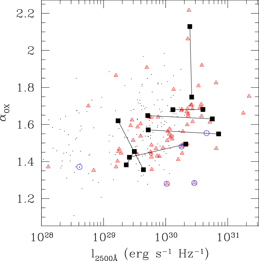
Figure 1.— $\alpha_{\mathrm{ox}}$  vs. optical 2500Å  log luminosity for the binary QSOs (black squares), with pair members linked by black lines. The comparison sample of 264 Chandra-detected SDSS QSOs with $z<1.2$ from Green et al. (2009) is also plotted, for which red triangles indicate spectroscopic redshifts, and blue circles show radio-loud objects.

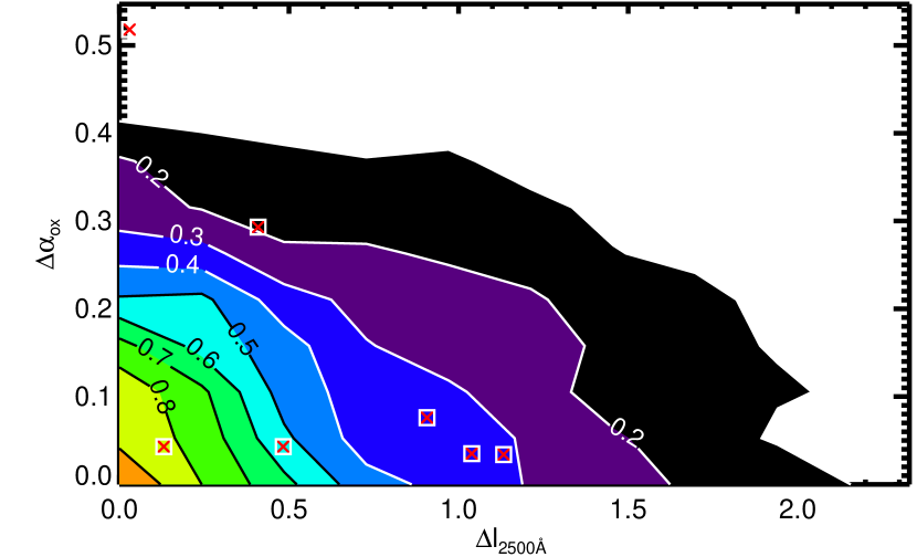
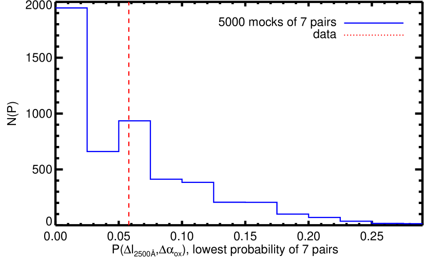
Figure 2.— LEFT: Distributions of $\Delta\,{\alpha_{\mathrm{ox}}}$, $\Delta\,l_{\mathrm{2500\,\AA}}$ for individual quasars and our 7 pairs of close quasars. The contours are the density of 5,000 pairs of quasars drawn at random from the 264 SDSS quasars in the ChaMP. Points are the 7 genuine pairs of quasars discussed in this paper. The most extreme of the 7 data points has a 7% probability of being drawn at random from the distribution of possible pairs of quasars. RIGHT: As our sample represents drawing 7 pairs of quasars, rather than just one pair, we repeat our experiment but testing instead the most improbable pair drawn at random in 5,000 samples of 7 mock pairs. We histogram the value of the contour (i.e. from the left-hand panel) for the most improbable of the 7 mock pairs. The dashed line is for the actual binary quasar sample data.

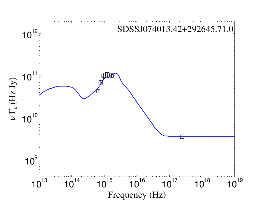
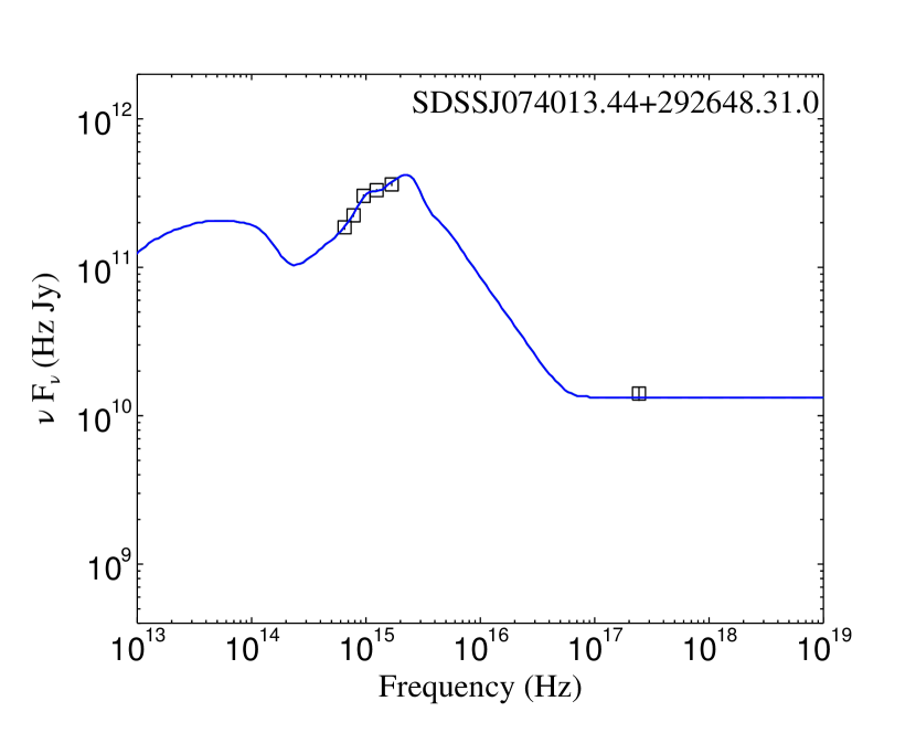
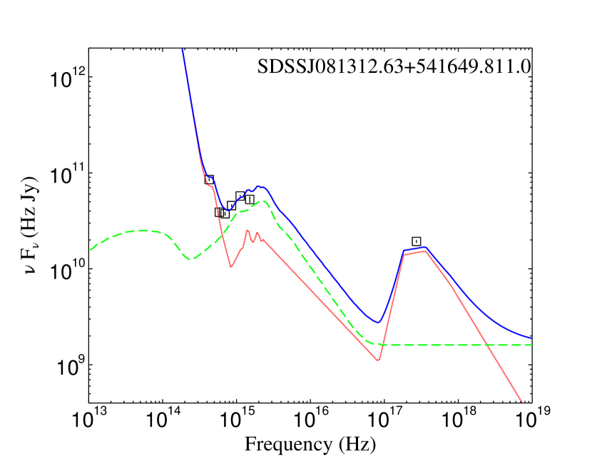
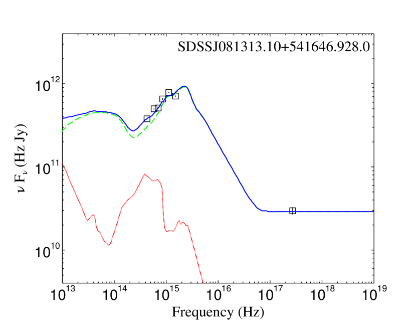
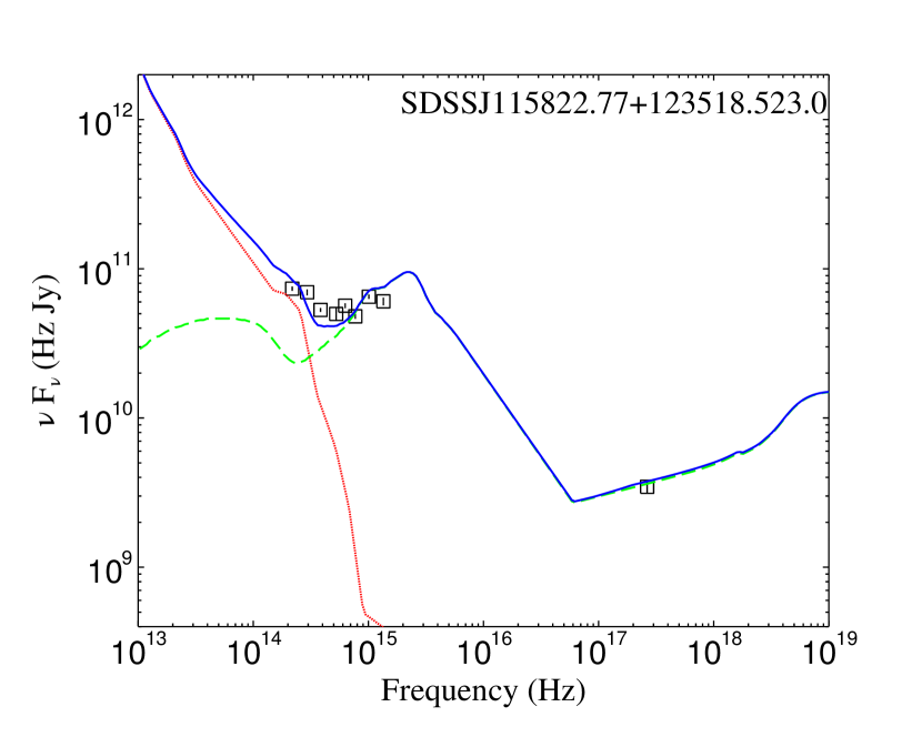
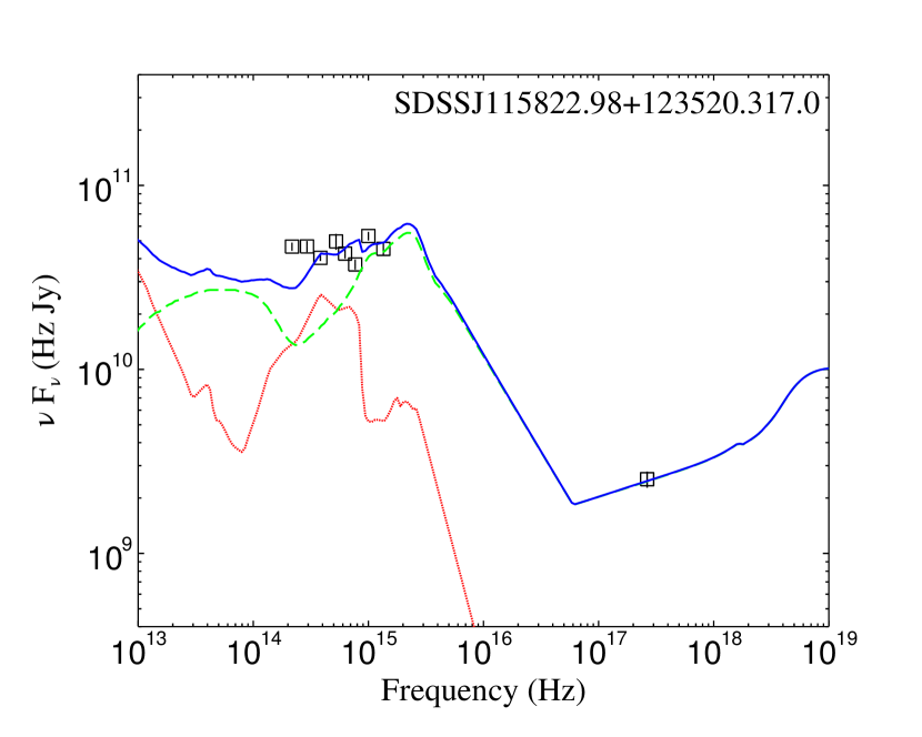
Figure 3.— Near-infrared to X-ray SEDs (Ruiz et al. 2010) in $\nu f_{\nu}$ for each of our quasar pairs. Solid blue lines show the total predicted SED. Green and red lines are the corresponding AGN and starburst templates used, respectively. Parameters for model fits are given in Table 4.

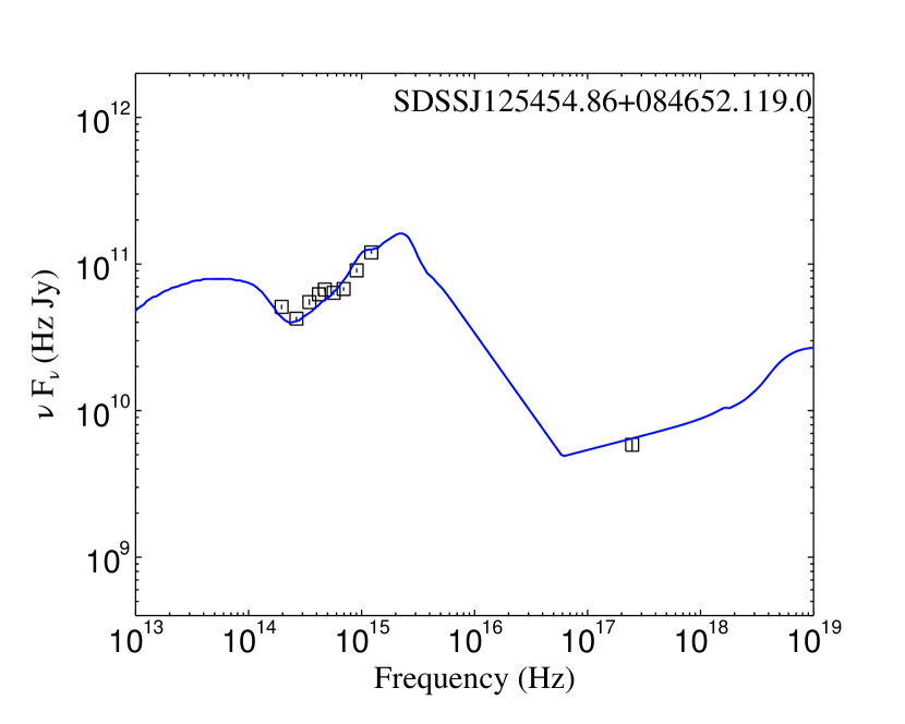
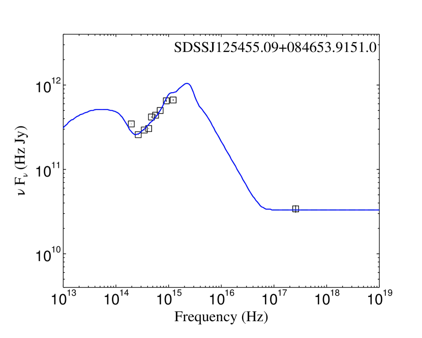
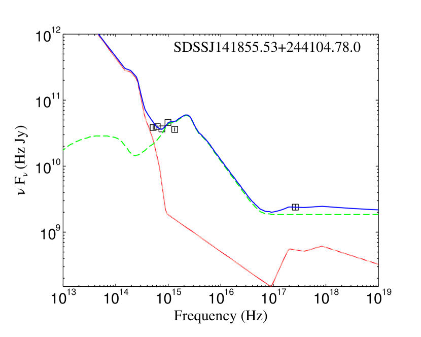
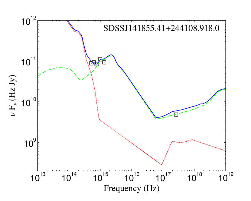
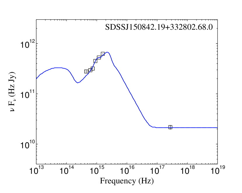
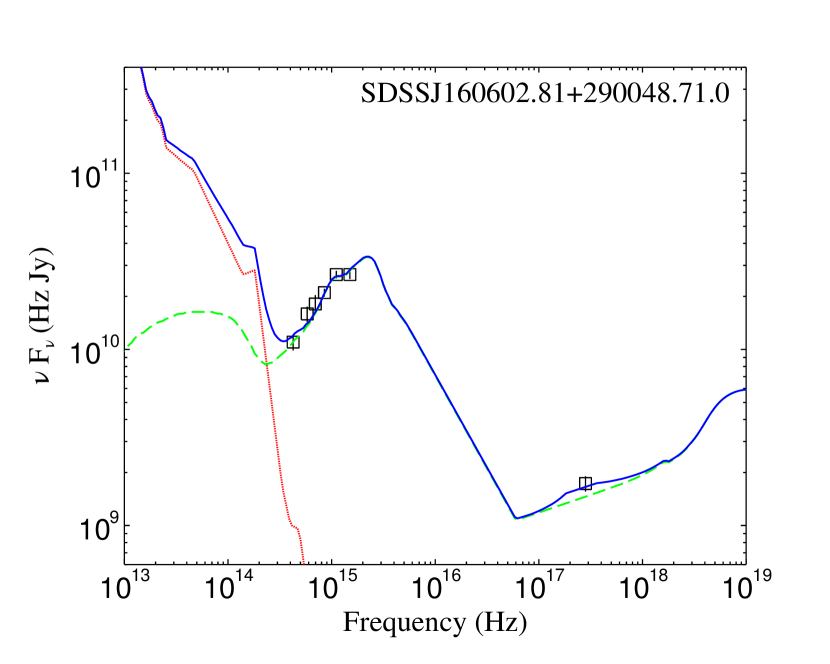
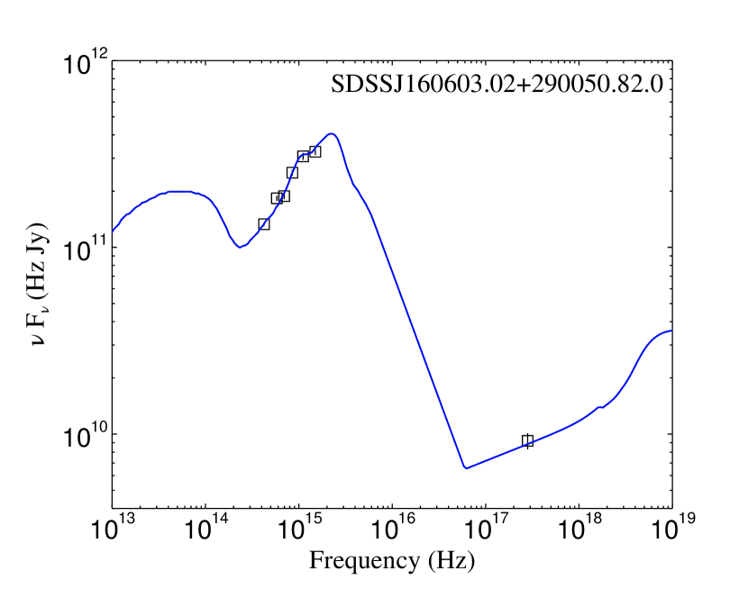
Figure 3.— Near-infrared to X-ray SEDs (Ruiz et al. 2010) in $\nu f_{\nu}$ for each of our quasar pairs. Solid blue lines show the total predicted SED. Green and red lines are the corresponding AGN and starburst templates used, respectively. Parameters for model fits are given in Table 4.

Figure 3.— Near-infrared to X-ray SEDs (Ruiz et al. 2010) in $\nu f_{\nu}$ for each of our quasar pairs. Solid blue lines show the total predicted SED. Green and red lines are the corresponding AGN and starburst templates used, respectively. Parameters for model fits are given in Table 4.

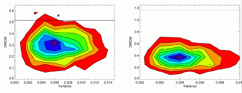
Figure 4.— Test of optical cluster significance. (LEFT) Contours from 10 to 90% in relative frequency show the distance-weighted ($i-z$) color measure (DWCM) vs. its variance for 1,000 random positions within the (2 deg) SDSS field of the QSO pair SDSS J1158+1235, calculated using the DWCM prescription described in § 6.2.2. The asterisk marks the DWCM and its variance calculated at the actual position of the quasar pair SDSS J1158+1235. The expected location ($i-z=0.98$) of the galaxy red sequence at $m^{\ast}$ based on the mean redshift $z\sim 0.878$ of the quasar pair is shown as a solid horizontal line, adopting the red sequence models of Kodama & Arimoto (1997). While the variance is typical ($\sim\,80\%$) for the field, the actual mean color (DWCM) is both unusual and close to the expected red-sequence color. (RIGHT) The DWCM vs. its variance for $(r-i)$ shows that the expected red-sequence value at the midpoint of the QSOs’ positions (asterisk) is entirely typical for random positions in the field, and far from the expected red-sequence color (horizontal line).

Table 1Chandra Close Binary Quasar Sample

Pair Name	ObsID	Exposure	$\theta$	$R_{p}$	Galactic $\mbox{N}_{\mbox{H}}$
		(sec)	(arcsec)	(kpc)	($10^{20}~{}\mbox{cm}^{-2}$)
SDSS J0740+2926	10312	20859	2.6	15.0	4.24
SDSS J0813+5416	10313	30625	5.0	26.9	4.21
SDSS J1158+1235	10314	30827	3.6	17.0	2.07
SDSS J1254+0846	10315	15967	3.8	15.4	1.92
SDSS J1418+2441	10316	29762	4.5	21.0	2.00
SDSS J1508+3328	10317	31317	2.9	16.0	1.51
SDSS J1606+2900	10318	12852	3.5	18.4	3.19

Table 2Chandra Close Binary Quasar Sample

SDSS NAME	$r$ mag	$z$	Counts	$\Gamma_{PL}$	$\Gamma_{PLAbs}$	$N_{H}^{z}~{}$	log $f_{X}$	log $l_{X}$	${\alpha_{\mathrm{ox}}}$
J074013.42+292645.7	19.47	0.978  H	82.4	1.85${}^{+0.20}_{-0.20}$	1.85${}^{+0.26}_{-0.20}$	$<$27	-13.527	25.993	1.583
J074013.44+292648.3	18.27	0.9803 S	288.5	2.24${}^{+0.11}_{-0.11}$	2.24${}^{+0.11}_{-0.11}$	$<$9	-13.044	26.589	1.540
J081312.63+541649.8	20.08	0.7814 K4m	195.7	2.51${}^{+0.15}_{-0.14}$	2.51${}^{+0.15}_{-0.14}$	$<$12	-13.414	26.006	1.426
J081313.10+541646.9	17.18	0.7792 S	2336.8	1.90${}^{+0.06}_{-0.06}$	1.93${}^{+0.04}_{-0.04}$	$<$1	-12.255	27.051	1.460
J115822.77+123518.5	19.85	0.5996 M08	367.7	2.26${}^{+0.10}_{-0.10}$	2.51${}^{+0.19}_{-0.18}$	18${}^{+11}_{-11}$	-13.098	26.017	1.335
J115822.98+123520.3	20.12	0.5957 M08	413.6	2.16${}^{+0.09}_{-0.09}$	2.14${}^{+0.16}_{-0.14}$	$<$9	-13.069	25.999	1.292
J125454.86+084652.1	19.43	0.4401 G	349.5	2.11${}^{+0.10}_{-0.10}$	2.11${}^{+0.10}_{-0.10}$	$<$2	-12.853	25.887	1.355
J125455.09+084653.9	17.08	0.4392 G	1795.5	2.04${}^{+0.04}_{-0.04}$	2.04${}^{+0.04}_{-0.04}$	$<$1	-12.129	26.597	1.431
J141855.41+244108.9	19.21	0.5728 S	864.9	1.94${}^{+0.06}_{-0.06}$	1.99${}^{+0.11}_{-0.10}$	$<$7	-12.692	26.305	1.282
J141855.53+244104.7	20.13	0.5751 M08	33.0	0.72${}^{+0.28}_{-0.28}$	1.6${}^{+0.60}_{-0.54}$	158${}^{+113}_{-87}$	-13.769	25.132	1.575
J150842.19+332802.6	17.80	0.8773 S	1040.9	2.10${}^{+0.06}_{-0.06}$	2.10${}^{+0.06}_{-0.06}$	$<$8	-12.670	26.807	1.514
J150842.21+332805.5	20.19	0.878  H	111.1	2.37${}^{+0.45}_{-0.40}$	2.61${}^{+0.37}_{-0.20}$	$<$27	-13.708	25.860	1.479
J160602.81+290048.7	18.35	0.7701 S	6.1	0.60${}^{+0.71}_{-0.73}$	2.1	$<$0.01	-14.491	24.844	2.129
J160603.02+290050.8	18.25	0.7692 M08	144.1	2.20${}^{+0.43}_{-0.42}$	2.44${}^{+0.17}_{-0.16}$	$<$6	-13.171	26.222	1.611

Table 3Chandra Binary Quasar Sample Near-Infrared Properties

SDSS Name	Exposure	$J_{S}$	err$J_{S}$	$J_{U}$	err$J_{U}$	Y	errY	H	errH	K	errK
J074013.42+292645.7	…	…	…	…	…	…	…	…	…	…	…
J074013.44+292648.3	…	…	…	…	…	…	…	…	…	…	…
J081312.63+541649.8	2610	17.869	0.034	…	…	…	…	…	…	…	…
J081313.10+541646.9	2610	18.744	0.061	…	…	…	…	…	…	…	…
J115822.77+123518.5	900	17.174	0.013	…	…	…	…	17.085	0.050	16.239	0.036
J115822.98+123520.3	900	17.411	0.016	…	…	…	…	17.515	0.074	16.732	0.056
J125454.86+084652.1	1260	18.098	0.061	17.925	0.045	18.424	0.034	17.066	0.022	16.129	0.029
J125455.09+084653.9	1260	16.063	0.010	16.079	0.009	16.505	0.008	15.433	0.006	14.327	0.007
J141855.41+244108.9	…	…	…	…	…	…	…	…	…	…	…
J141855.53+244104.7	…	…	…	…	…	…	…	…	…	…	…
J150842.19+332802.6	630	16.551	0.058	16.629	0.012	…	…	…	…	…	…
J150842.21+332805.5	630	18.473	0.031	18.463	0.063	…	…	…	…	…	…
J160602.81+290048.7	…	…	…	17.398	0.023	…	…	…	…	…	…
J160603.02+290050.8	…	…	…	17.369	0.022	…	…	…	…	…	…

Table 4Quasar Spectral Energy Distribution Fit Results

SDSS Name	log LBol	$J_{AGN}$	$J_{SB}$	$P_{IRX}$	$P_{Bol}$
J074013.42+292645.7	46.362	QSO	…	100/0	100/0
J074013.44+292648.3	46.909	QSO	…	100/0	100/0
J081312.63+541649.8	48.159	QSO	M82	71/29	$<$10/$>$90
J081313.10+541646.9	47.087	QSO	NGC7714	79/21	79/21
J115822.77+123518.5	47.185	LDQSO	IRAS 12112+0305	74/26	$<$10/$>$90
J115822.98+123520.3	45.770	LDQSO	NGC7714	58/42	58/42
J125454.86+084652.1	45.787	LDQSO	…	100/0	100/0
J125455.09+084653.9	46.457	QSO	…	100/0	100/0
J141855.41+244108.9	48.009	LDQSO	IRAS 12112+0305	80/20	$<$10/$>$90
J141855.53+244104.7	47.713	QSO	IRAS 12112+0305	76/24	$<$10/$>$90
J150842.19+332802.6	47.013	QSO	…	100/0	100/0
J150842.21+332805.5	48.127	LDQSO	IRAS 12112+0305	77/23	$<$10/$>$90
J160602.81+290048.7	48.225	LDQSO	M82	68/32	$<$10/$>$90
J160603.02+290050.8	46.641	LDQSO	…	100/0	100/0

References

- Aldcroft & Green (2003) Aldcroft, T. L., & Green, P. J. 2003, ApJ, 592, 710
- Allen et al. (2001) Allen, S. W., et al. 2001, MNRAS, 324, 842
- Avni & Tananbaum (1982) Avni, Y., & Tananbaum, H. 1982, ApJ, 262, L17
- Barkhouse et al. (2006) Barkhouse, W. A., et al. 2006, ApJ, 645, 955
- Bertin (2006) Bertin, E. 2006, SWarp ver. 2.16 User’s Guide (Paris: Terapix), http://terapix.iap.fr/IMG/pdf/swarp.pdf
- Bertin & Arnouts (1996) Bertin, E., & Arnouts, S. 1996, A&AS, 117, 393
- Bianchi et al. (2008) Bianchi, S., Chiaberge, M., Piconcelli, E., Guainazzi, M., & Matt, G. 2008, MNRAS, 386, 105
- Bogdanović et al. (2009) Bogdanović, T., Eracleous, M., & Sigurdsson, S. 2009, ApJ, 697, 288
- Boroson & Lauer (2009) Boroson, T.A. & Lauer, T.R. 2009, Nature, 458, 53
- Cash (1979) Cash, W. 1979, ApJ, 228, 939
- Cheung (2007) Cheung, C. C. 2007, AJ, 133, 2097
- Chornock et al. (2010) Chornock, R., et al. 2010, ApJ, 709, L39
- Cisternas et al. (2011) Cisternas, M., et al. 2011, ApJ, 726, 57
- Civano et al. (2010) Civano, F., et al. 2010, ApJ, 717, 209
- Comerford et al. (2009) Comerford, J. M., et al. 2009a, ApJ, 698, 956
- Croom et al. (2005) Croom, S. M. et al. 2005, MNRAS, 356, 415
- Cutri et al. (2003) Cutri, R. M., et al. 2003, The IRSA 2MASS All-Sky Point Source Catalog, NASA/IPAC Infrared Science Archive. http://irsa.ipac.caltech.edu/applications/Gator/
- Dickey & Lockman (1990) Dickey, J. M., & Lockman, F. J. 1990, Annu. Rev. Astron. Astrophys., 28, 215
- Djorgovski et al. (1987) Djorgovski, S. G., et al. 1987, ApJ, 321, L17
- Djorgovski (1991) Djorgovski, S. 1991, The Space Distribution of Quasars, 21, 349
- Dotti et al. (2009) Dotti, M., Montuori, C., Decarli, R., Volonteri, M., Colpi, M., & Haardt, F. 2009, MNRAS, 398, L73
- Ellison et al. (2010) Ellison, S. L., Patton, D. R., Simard, L., McConnachie, A. W., Baldry, I. K., & Mendel, J. T. 2010, MNRAS, 407, 1514
- Ellison et al. (2008) Ellison, S. L., Patton, D. R., Simard, L., & McConnachie, A. W. 2008, AJ, 135, 1877
- Elvis et al. (1994) Elvis, M., et al., 1994, ApjS, 95, 1
- Fan et al. (2001) Fan, X. et al., 2001, AJ 122, 1833
- Fan et al. (2006) Fan, X., et al. 2006, AJ, 131, 1203
- Ferrarese & Merritt (2000) Ferrarese, L., & Merritt, D. 2000, ApJ, 539, L9
- Fu et al. (2010) Fu, H., Myers, A. D., Djorgovski, S. G., & Yan, L. 2011, ApJ, in press (arXiv:1009.0767)
- Fukugita et al. (1996) Fukugita, M., Ichikawa, T., Gunn, J.E., Doi, M., Shimasaku, K., Schneider, D.P. 1996, AJ, 111, 1748
- Gallagher et al. (2006) Gallagher, S. C., Brandt, W. N., Chartas, G., Priddey, R., Garmire, G. P., & Sambruna, R. M. 2006, ApJ, 644, 709
- Gallagher et al. (2007) Gallagher, S. C., Hines, D. C., Blaylock, M., Priddey, R. S., Brandt, W. N., & Egami, E. E. 2007, ApJ, 665, 157
- Gallo et al. (2008) Gallo, E., Treu, T., Jacob, J., Woo, J.-H., Marshall, P. J., & Antonucci, R. 2008, ApJ, 680, 154
- Gladders & Yee (2000) Gladders, M. D., & Yee, H. K. C. 2000, AJ, 120, 2148
- Green et al. (1995) Green, P. J., et al. 1995, ApJ, 450, 51
- Green et al. (2001b) Green, P. J., Aldcroft, T. L., Mathur, S., Wilkes, B. J., & Elvis, M. 2001, ApJ, 558, 109
- Green et al. (2002) Green, P. J., et al. 2002, ApJ, 571, 721
- Green et al. (2004) Green, P. J., et al. 2004, ApJS, 150, 43
- Green (2005) Green, P. J., Infante, L., Lopez, S., Aldcroft, T. L., & Winn, J. N. 2005, ApJ, 630, 142
- Green et al. (2009) Green, P. J. et al. 2009, ApJ, 690, 644
- Green et al. (2010) Green, P. J., Myers, A. D., Barkhouse, W. A., Mulchaey, J. S., Bennert, V. N., Cox, T. J., & Aldcroft, T. L. 2010, ApJ, 710, 1578
- Greene & Ho (2007) Greene, J. E., & Ho, L. C. 2007, ApJ, 670, 92
- Gültekin et al. (2009) Gültekin, K., et al. 2009, ApJ, 698, 198
- Haggard et al. (2010) Haggard, D., Green, P. J., Anderson, S. F., Constantin, A., Aldcroft, T. L., Kim, D.-W.,
- Hatziminaoglou et al. (2010) Hatziminaoglou, E., et al., 2010, A&A, 518, 33
- Heckman et al. (2004) Heckman, T. M., Kauffmann, G., Brinchmann, J., Charlot, S., Tremonti, C., & White, S. D. M. 2004, ApJ, 613, 109
- Hennawi et al. (2006) Hennawi, J. F., et al. 2006, AJ, 131, 1
- Hennawi et al. (2010) Hennawi, J. et al. 2010, ApJ, 719, 1672
- Hernquist (1989) Hernquist, L. 1989, Nature, 340, 687
- Ho et al. (1997) Ho, L. C., Filippenko, A. V., & Sargent, W. L. W. 1997, ApJ, 487, 568
- Hopkins et al. (2005) Hopkins, P., et al., 2005, ApJ, 630, 705
- Hopkins et al. (2007a) Hopkins, P., et al., 2007a, ApJ, 654, 731
- Hopkins et al. (2008) Hopkins, P. F., Hernquist, L., Cox, T. J., & Kereš, D. 2008, ApJS, 175, 356
- Hopkins et al. (2010) Hopkins, P. F., et al. 2010, ApJ, 724, 915
- Iwasawa et al. (2001) Iwasawa, K., Fabian, A. C., & Ettori, S. 2001, MNRAS, 321, L15
- Kalfountzou et al. (2010) Kalfountzou, E., et al., 2010, MNRAS in press (astro-ph/1005.4353)
- Kauffmann & Haehnelt (2000) Kauffmann, G. & Haehnelt, M. 2000, MNRAS, 311, 576
- Kauffmann et al. (2003) Kauffmann, G., et al. 2003, MNRAS, 346, 1055
- Kochanek et al. (1999) Kochanek, C. S., Falco, E., Munoz, J. A. 1999, ApJ, 510, 590
- Kodama & Arimoto (1997) Kodama, T., & Arimoto, N. 1997, A&Ap, 320, 41
- Komossa et al. (2003) Komossa, S., et al. 2003, ApJ, 582, L15
- Komossa et al. (2008) Komossa, S., Zhou, H., & Lu, H. 2008, ApJL, 678, L81
- Lauer & Boroson (2009) Lauer, T.R. & Boroson, T.A. 2009, ApJ,703, 90
- Liu (2004) Liu, F. K. 2004, MNRAS, 347, 1357
- Liu et al. (2010) Liu, X., Shen, Y., Strauss,
- Lusso et al. (2010) Lusso, E., et al. 2010, A&A, 512, A34
- Lutz et al. (2008) Lutz, D., et al., 2008, ApJ, 684, 853
- Lutz et al. (2010) Lutz, D., et al., 2010, ApJ, 712, 1287
- Martini et al. (2009) Martini, P., Sivakoff, G. R., & Mulchaey, J. S. 2009, ApJ, 701, 66
- Merloni & Heinz (2008) Merloni, A. & Heinz, S. 2008, MNRAS 388, 1011
- Merritt & Ekers (2002) Merritt, D., & Ekers, R. D. 2002, Science, 297, 1310
- Mink (1997) Mink, D. J. 1997, Astronomical Data Analysis Software and Systems VI, 125, 249
- Morrison & McCammon (1983) Morrison, R, McCammon D. 1983, ApJ, 270, 119
- Mortlock et al. (1999) Mortlock, D. J., Webster, R. L., & Francis, P. J. 1999, MNRAS, 309, 836
- Mortlock et al. (2011) Mortlock, D. J., et al. 2011, Nature, 474, 616
- Mukai (1993) Mukai, K. 1993, Legacy, 3, 21
- Mullis et al. (2004) Mullis, C. R., et al. 2004, ApJ, 607, 175
- Myers et al. (2006) Myers, A. D. et al. 2006, ApJ, 638, 622
- Myers et al. (2007a) Myers, A. D., 2007, ApJ, 658, 85
- Myers et al. (2007b) Myers, A. D., 2007, ApJ, 658, 99
- Myers et al. (2008) Myers, A. D., et al. 2008, ApJ, 678, 635
- Porciani et al. (2004) Porciani, C., Magliocchetti, M., & Norberg, P. 2004, MNRAS, 355, 1010
- Richards et al. (2006) Richards et al. 2006, ApJS, 166, 470
- Richards et al. (2009) Richards, G. T., et al. 2009, ApJS, 180, 67
- Ross et al. (2009) Ross, N. P., et al. 2009, ApJ, 697, 1634
- Rudnick et al. (2001) Rudnick, G., et al. 2001, AJ, 122, 2205
- Ruiz et al. (2007) Ruiz, A., et al., 2007, A&A, 471, 775
- Ruiz et al. (2010) Ruiz, A., Miniutti, G., Panessa, F., & Carrera, F. J. 2010, A&A, 515, A99
- Russell et al. (2010) Russell, H. R., Fabian, A. C., Sanders, J. S., Johnstone, R. M., Blundell, K. M., Brandt, W. N., & Crawford, C. S. 2010, MNRAS, 402, 1561
- Ryan et al. (2008) Ryan, R. E., Jr., Cohen, S. H., Windhorst, R. A., & Silk, J. 2008, ApJ, 678, 751
- Saracco et al. (2001) Saracco, P., et al. 2001, A&A, 375, 1
- Schawinski et al. (2009) Schawinski, K., et al., 2009, ApJ, 692, 19
- Schawinski et al. (2010) Schawinski, K., et al. 2010, ApJ, 711, 284
- Shen et al. (2007) Shen Y. et al., 2007, AJ, 133, 2222
- Shen et al. (2010a) Shen, Y., et al. 2010, ApJ, 719, 1693
- Shen et al. (2010b) Shen, Y., Liu, X., Greene, J., & Strauss, M. 2010, arXiv:1011.5246
- Shi et al. (2008) Shi, Y., Rieke, G., Donley, J., Cooper, M., Willmer, C., & Kirby, E. 2008, ApJ, 688, 794
- Shields et al. (2009) Shields, G. A., et al. 2009, ApJ, 707, 936
- Siemiginowska et al. (2010) Siemiginowska, A., et al. 2010, ApJ, 722, 102
- Sillanpaa et al. (1988) Sillanpaa, A., Haarala, S., Valtonen, M. J., Sundelius, B., & Byrd, G. G. 1988, ApJ, 325, 628
- Silverman et al. (2008) Silverman, J. D., et al. 2008, ApJ, 679, 118
- Sivakoff et al. (2008) Sivakoff, G. R., Martini, P., Zabludoff, A. I., Kelson, D. D., & Mulchaey, J. S. 2008, ApJ, 682, 803
- Skrutskie et al. (2006) Skrutskie, M. F., et al. 2006, AJ, 131, 1163
- Smith et al. (2010) Smith, K. L., Shields, G. A., Bonning, E. W., McMullen, C. C., Rosario, D. J., & Salviander, S. 2010, ApJ, 716, 866
- Sobolewska et al. (2011) Sobolewska, M. A., Siemiginowska, A & Gierlinski, M. 2011, MNRAS, 413, 2259
- Soltan (1982) Soltan, A. 1982, MNRAS, 200, 115
- Springel (2005) Springel, V. et al. 2005, Nature, 435, 629
- Staniszewski et al. (2009) Staniszewski, Z., Ade, P. A. R., Aird, K. A., et al. 2009, ApJ, 701, 32
- Steffen et al. (2006) Steffen, A. T., Strateva, I., Brandt, W. N., Alexander, D. M., Koekemoer, A. M., Lehmer, 2006, AJ, 131, 2826
- Strand et al. (2008) Strand, N. E., Brunner, R. J., & Myers, A. D. 2008, ApJ, 688, 180
- Strateva et al. (2003) Strateva, I. V., et al. 2003, AJ, 126, 1720
- Symeonidis et al. (2010) Symeonidis, M., et al., 2010, MNRAS, 403, 1474
- Tang & Grindlay (2009) Tang, S., & Grindlay, J. 2009, ApJ, 704, 1189
- Trichas et al. (2009) Trichas, M., et al., 2009, MNRAS, 399, 663
- Trichas et al. (2010) Trichas, M., et al., 2010, MNRAS, 405, 2243
- Tang et al. (2007) Tang, S. M., Zhang, S. N., & Hopkins, P. F. 2007, MNRAS, 377, 1113
- Valtonen et al. (2011) Valtonen, M. J., Lehto, H. J., Takalo, L. O., & Sillanpää, A. 2011, ApJ, 729, 33
- Vanderlinde et al. (2010) Vanderlinde, K., Crawford, T. M., de Haan, T., et al. 2010, ApJ, 722, 1180
- Villforth et al. (2010) Villforth, C., et al. 2010, MNRAS, 402, 2087
- Vivek et al. (2009) Vivek, M., Srianand, R., Noterdaeme, P., Mohan, V., & Kuriakosde, V. C. 2009, MNRAS, 400, L6
- Wang et al. (2009) Wang, J.-M., Chen, Y.-M., Hu, C., Mao, W.-M., Zhang, S., & Bian, W.-H. 2009, ApJ, 705, L76
- Weinstein et al. (2004) Weinstein, M. A., et al. 2004, ApJS, 155, 243
- Wilkes et al. (1994) Wilkes, B. J. et al. 1994, ApJS, 92, 53
- Wilms et al. (2000) Wilms, J., Allen, A., & McCray, R. 2000, ApJ, 542, 914
- Wright et al. (2010) Wright, E. L., et al. 2010, AJ, 140, 1868
- Wrobel & Laor (2009) Wrobel, J. M., & Laor, A. 2009, ApJ, 699, L22
- Xu & Komossa (2009) Xu, D., & Komossa, S. 2009, ApJ, 705, L20
- Yee & Ellingson (1993) Yee, H. K. C., & Ellingson, E. 1993, ApJ, 411, 43
- York et al. (2000) York, D. G., et al. 2000, AJ, 120, 1579
- Yuan et al. (1998) Yuan, W., Siebert, J., & Brinkmann, W. 1998, A&A, 334, 498
- Zezas et al. (2003) Zezas, A., Ward, M. J., & Murray, S. S. 2003, ApJL, 594, L31