The enigmatic core L1451-mm: a first hydrostatic core? or a hidden VeLLO?

Abstract

We present the detection of a dust continuum source at 3-mm (CARMA) and 1.3-mm (SMA), and ${\rm{}^{12}CO}$ (2–1) emission (SMA) towards the L1451-mm dense core. These detections suggest a compact object and an outflow where no point source at mid-infrared wavelengths is detected using Spitzer. An upper limit for the dense core bolometric luminosity of 0.05 $L_{\odot}$ is obtained. By modeling the broadband SED and the continuum interferometric visibilities simultaneously, we confirm that a central source of heating is needed to explain the observations. This modeling also shows that the data can be well fitted by a dense core with a YSO and disk, or by a dense core with a central First Hydrostatic Core (FHSC). Unfortunately, we are not able to decide between these two models, which produce similar fits. We also detect ${\rm{}^{12}CO}$ (2–1) emission with red- and blue-shifted emission suggesting the presence of a slow and poorly collimated outflow, in opposition to what is usually found towards young stellar objects but in agreement with prediction from simulations of a FHSC. This presents the best candidate, so far, for a FHSC, an object that has been identified in simulations of collapsing dense cores. Whatever the true nature of the central object in L1451-mm, this core presents an excellent laboratory to study the earliest phases of low-mass star formation.

1. Introduction

Star formation takes place in the densest regions of molecular clouds, usually referred to as dense cores. The parental molecular clouds show highly supersonic velocity dispersions, while the dense cores show subsonic levels of turbulence (Goodman et al., 1998; Caselli et al., 2002). Recently, Pineda et al. (2010) showed that this transition in velocity dispersion is extremely sharp and it can be observed in $\rm NH_{3}$ (1,1) (see also Pineda et al. 2011, in prep).

Starless dense cores represent the initial conditions of star formation. Crapsi et al. (2005) identify a sample of starless cores which show a number of signs indicating that they may be “evolved” and thus close to forming a star.

In the earliest phases of star formation a starless core undergoes a gravitational collapse. Increasing central densities will result in an increase in dust optical depth and thus cooling within the core will not be as efficient as in the earliest phases. This increases the gas temperature and generates more pressure. The first numerical simulation to study the formation of a protostar from an isothermal core (Larson, 1969), revealed the formation of a central adiabatic core, defined as a “first hydrostatic core” (hereafter FHSC). This FHSC would then accrete more mass and undergo adiabatic contraction until $\rm H_{2}$ is dissociated, at which point it begins a second collapse until it forms a “second hydrostatic core,” which is the starting point for protostellar objects.

A few FHSC candidates have been suggested in the past. Belloche et al. (2006) present single dish observations of the Cha-MMS1 dense core which combined with detections at 24 and 70 $\mu$m with Spitzer suggest the presence of a first hydrostatic core or an extremely young protostar (see also Belloche et al., 2011). Chen et al. (2010) present SMA observations of the continuum at 1.3-mm and ${\rm{}^{12}CO}$ (2–1) line in the L1448 region located in the Perseus cloud where no Spitzer (IRAC or MIPS) source is detected. They detect a weak continuum source and a well collimated high-velocity outflow is observed in ${\rm{}^{12}CO}$ (2–1). Chen et al. (2010) analyze different scenarios to explain the observations and conclude that a FHSC provide the best case, however, no actual modeling of the interferometric observations is presented. Recently, Enoch et al. (2010) present CARMA 3-mm continuum and deep Spitzer 70 $\mu$m observations of another FHSC candidate (Per-Bolo 58) in the NGC1333 region also located in the Perseus cloud. In these observations they detect a weak source in the 3-mm continuum and 70 $\mu$m. Enoch et al. (2010) simultaneously modeled the broadband SED and the visibilities, allowing them to conclude that the best explanation for the central source is a FHSC. Dunham et al. (2011, submitted) present SMA 1.3-mm observations which reveal a collimated slow molecular outflow using ${\rm{}^{12}CO}$ (2–1) emission.

Another class of low luminosity objects has been identified thanks to Spitzer: Very Low Luminosity Objects (VeLLOs, e.g., Young et al., 2004; Bourke et al., 2005; Dunham et al., 2006), some of which are found within evolved cores (as classified by Crapsi et al., 2005). These objects have low intrinsic luminosities ($L<0.1~{}{L_{\odot}}$) and are embedded in a dense core (di Francesco et al., 2007). As VeLLOs have only recently been revealed by Spitzer (Dunham et al., 2008), it is not yet clear whether these are sub-stellar objects that are still forming, or low-mass protostars in a low-accretion state.

Broadband SED modeling of VeLLOs suggest that these sources can be explained as embedded YSOs with a surrounding disk. In the case of IRAM 04191+1522 (hereafter IRAM 04191), continuum observations using the IRAM Plateau de Bure interferometer (PdBI) were interpreted by Belloche et al. (2002) as produced from the dense core’s inner part without the need for a disk.

Recently, Maury et al. (2010) presented high-resolution PdBI observations towards a sample of 5 Class 0 sources to study the binary fraction in the early stages of star formation. Their sample includes two previously known VeLLOs: L1521-F and IRAM 04191. Dust continuum emission is detected toward both objects, which may arise from either a circumstellar disk or from the inner parts of the envelope. Lack of detailed modeling of the SED or visibilities in these sources makes it hard to distinguish between these two scenarios.

This paper presents observations of L1451-mm, a low-mass core without any associated mid-infrared source in which we have detected compact thermal dust emission and a molecular outflow, along with models constructed to derive the properties of this object. In §2 we discuss previous observations of L1451-mm. In §3 presents data used in this paper. In §4 we present the analysis of the observations and radiative transfer models to reproduce the observed spectral energy distribution (SED) and the continuum visibilities to constrain the physical conditions of the source. Finally, we present our conclusions in §5.

2. L1451-mm

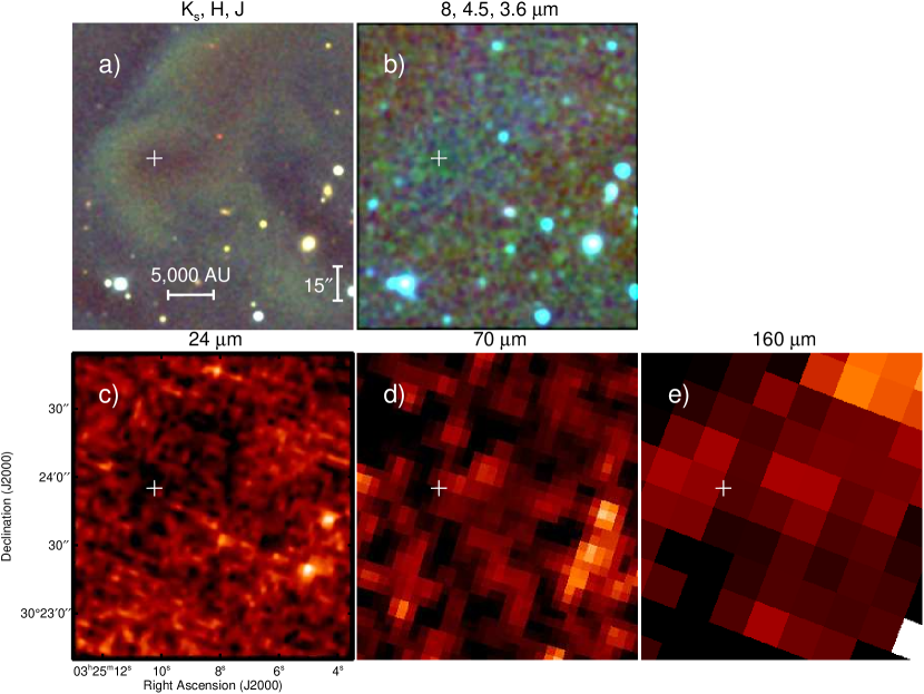
Figure 1.— Summary of observations available towards L1451-mm between 1 and 160$\mu$m. (a) $K_{s}$, $H$ and $J$ three color image, red, green, and blue respectively. The white cross shows the central position observed with the SMA. (b) IRAC-4, -2 and -1 three color image, red, green, and blue respectively. (c) MIPS-1 monochrome, (c) MIPS-2 monochrome; and (d) MIPS-3 monochrome figures. No point source is detected in any of the images.

L1451-mm (also known as Per-Bolo 2; Enoch et al., 2006) is a cold dense core in the L1451 Dark Cloud located in the Perseus Molecular Cloud Complex. Here we assume that Perseus is at a distance of $\sim 250$ pc (Cernis, 1990; Hirota et al., 2008), which is consistent with those used by previous works. L1451-mm is detected in 1.1 mm dust continuum with Bolocam at 31″ resolution, and its estimated mass is 0.36 $M_{\odot}$ from the Gaussian fit by Enoch et al. (2006) with major and minor FWHMs of $33\arcsec$ and $54\arcsec$, respectively. However, the core is too faint to be identified by the SCUBA surveys at 850 $\mu$m of the Perseus Cloud (Hatchell et al., 2005; Kirk et al., 2006; Sadavoy et al., 2010).

Figure 1 presents a summary of the observations pre-dating this work towards L1451-mm. Foster & Goodman (2006) presented deep Near-IR observations ($J$ $H$ $K_{s}$) of L1451-mm which show only heavy obscuration, and no evidence for a point source. Establishing upper limits for this non-detection was complicated by the presence of extended bright structure (i.e., cloudshine) around the edge of L1451-mm. We estimate an upper limit by inserting synthetic stars with a range of magnitudes (in 0.1 magnitude steps) and appropriate FWHM at the central position. We ran Source Extractor (Bertin & Arnouts, 1996) on these synthetic images using a 2.25$\arcsec$ radius aperture and established the input magnitude at which a 3$\sigma$ source was successfully extracted.

This core is classified as “starless” by Enoch et al. (2008), because no point source is detected in Spitzer IRAC and MIPS images (Jørgensen et al., 2006; Rebull et al., 2007). Since the IRAC images do not contain significant extended emission we measured the flux in a 2.5$\arcsec$ radius aperture centered on the central position of L1451-mm with a background annulus of 2.5 to 7.5$\arcsec$ using the IRAF phot routine and applied the aperture correction factor for this configuration from the IRAC instrument handbook. All fluxes measured this way were within 2$\sigma$ of zero (fluxes were both positive and negative). For MIPS we used the smallest aperture with a well-defined aperture correction factor, which is 16$\arcsec$. Both MIPS1 and MIPS2 were consistent with zero flux while MIPS3 was a weak (2.7$\sigma$) detection. A summary of the photometric results is presented in Table 1.

Table 1Photometry of L1451-mm

Filter	Wavelength	Flux	Aperture
	($\mu$m)	(mJy)	(arcsec)
$J$	1.25	$<0.006$	2.25
$H$	1.65	$<0.0048$	2.25
$K_{s}$	2.17	$<0.0099$	2.25
IRAC1	3.6	$<0.048$	2.5
IRAC2	4.5	$<0.012$	2.5
IRAC3	5.8	$<0.060$	2.5
IRAC4	8.0	$<0.030$	2.5
MIPS1	24.0	$<1.5$	16
MIPS2	70.0	$<72$	16
MIPS3	160.	$880\pm 330$	16
IRAM	1200	$70\pm 7$	16.8

Note. — Upper limits used are 3-$\sigma$ limits.

Given the lack of detectable emission at Spitzer wavelengths, and using the correlation between 70$\mu$m and intrinsic YSO luminosity determined by Dunham et al. (2008), an upper limit of $L<1.6\times 10^{-2}\,{L_{\odot}}$ on the luminosity of a source embedded within L1451-mm is determined.

For a given SED, two quantities can be calculated to describe it: bolometric luminosity, $L_{bol}$, and bolometric temperature, $T_{bol}$. The bolometric luminosity is calculated through integration of the SED ($S_{\nu}$) over the observed frequency range,

$$L_{bol}=4\pi\,d^{2}\int S_{\nu}d\nu~{},$$ (1)

while the bolometric temperature is calculated following Myers & Ladd (1993),

$$T_{bol}=1.25\times 10^{-11}\left(\frac{\langle\nu\rangle}{{\rm Hz}}\right)\,{\rm K}~{},$$ (2)

where

$$\langle\nu\rangle=\frac{\int\nu\,S_{\nu}d\nu}{\int S_{\nu}d\nu}~{}.$$ (3)

For L1451-mm, if the upper limits are used as measurements, then we obtain $L_{bol}\leq 0.05\,{L_{\odot}}$ and $T_{bol}\leq 30$ K (see Dunham et al., 2008; Enoch et al., 2009b, for discussions on the uncertainties in calculating $T_{bol}$ and $L_{bol}$). This bolometric luminosity is lower than any of the Class 0 objects studied by Enoch et al. (2009b) in Serpens, Ophiuchus and Perseus Molecular Clouds; and also it is fainter than any of the VeLLOs with (sub-)millimeter wavelength observations studied by Dunham et al. (2008).

Pineda et al. (2011 in prep) present $\rm NH_{3}$ (1,1) and (2,2) line maps observed with the 100-meter Green Bank Telescope. From these observations they derive an almost constant (within a $\approx 1\arcmin$ radius) kinetic temperature, $T_{kin}\approx 9.7$ K, and velocity dispersion, $\sigma_{v}\approx 0.15\,{{\rm km\,s^{-1}}}$, showing no evidence for heating from a central source.

3. Observations

3.1. Single dish continuum observations

Dust continuum observations at 1.2-mm were taken using MAMBO at IRAM 30m telescope, under good weather ($\tau_{1.2mm}=0.1-0.2$). The data reduction was carried out using MOPSI, with parameters optimized for extended sources. The observations are convolved with a 15″ Gaussian kernel, while the flux unit is in Jy per 11″ beam. The rms noise level is 1 mJy per 11″ beam, and the map for the core studied is shown in Figure 2.

3.2. VLA Observations

Observations were carried out with the Very Large Array (VLA) of the National Radio Astronomy Observatory on January 10, 2006 (project AA300). The $\rm NH_{3}$ $(J,K)=(1,1)$ and $(2,2)$ inversion transitions were observed simultaneously (see Table 2 for a summary of the correlator configuration used). At this frequency the primary beam of the antennas is about $1.9\arcmin$. The array was in the compact (D) configuration, the bandwidth was $1.56$ MHz, and the channel separation was 12.2 kHz (corresponding to 0.154 ${\rm km\,s^{-1}}$). This configuration is centered at the main hyperfine component and it also covers the inner pair of satellite lines for $\rm NH_{3}$ (1,1).

Table 2VLA Spectral Setup: 23 GHz Setting

			Resolution	Frequency
Molecule	Transition	Chan.	(${\rm km\,s^{-1}}$)	(GHz)
$\rm NH_{3}$	$(1,1)$	63	0.1544	23.694495
$\rm NH_{3}$	$(2,2)$	63	0.1542	23.722733

The bandpass and absolute flux calibrator was the quasar 0319+415 (3C84) with a calculated flux density of $10.6$ Jy at $1$ cm, and the phase and amplitude calibrator was 0336+323. The raw-data were reduced using CASA image processing software. The signal from each baseline was inspected, and baselines showing spurious data were removed prior to imaging. The images were created using multi-scale clean (scales [8,24,72] arcsec and smallscalebias=0.8) with a robust parameter of $0.5$ and tapering the image with a 8$\arcsec$ Gaussian to increase the signal-to-noise. Each channel was cleaned separately according to the spatial distribution of the emission, using a circular beam of $8\arcsec$. Table 3 lists relevant information on the maps used.

Table 3Parameters of Interferometric Maps

Map	Array	Beam	rms
$\rm NH_{3}$ (1,1)	VLA	8″$\times$8″($0\arcdeg$)	3 m$\rm Jy\,beam^{-1}$  channel-1
$\rm NH_{3}$ (2,2)	VLA	8″$\times$8″($0\arcdeg$)	3 m$\rm Jy\,beam^{-1}$  channel-1
$\rm NH_{2}D$ ($1_{11}$–$1_{01}$)	CARMA	9.2″$\times$7.6″($+72.3\arcdeg$)	90 m$\rm Jy\,beam^{-1}$  channel-1
$\rm N_{2}H^{+}$ (1–0)	CARMA	5.2″$\times$4.3″($-73\arcdeg$)	80 m$\rm Jy\,beam^{-1}$  channel-1
3-mm continuum	CARMA	5.4″$\times$4.8″($-77\arcdeg$)	0.5 m$\rm Jy\,beam^{-1}$
${\rm{}^{12}CO}$ (2–1)	SMA	1.35″$\times$0.96″($+80.9\arcdeg$)	40 m$\rm Jy\,beam^{-1}$  channel-1
1.3-mm continuum	SMA	1.23″$\times$0.88″($+85.6\arcdeg$)	0.5 m$\rm Jy\,beam^{-1}$

3.3. CARMA observations

Continuum observations in the 3-mm window were obtained with CARMA, a 15-element interferometer consisting of nine 6.1-meter antennas and six 10.4-meter antennas, between April and September 2008. The CARMA correlator records signals in three separate bands, each with an upper and lower sideband. We configured one band for maximum bandwidth (468 MHz with 15 channels) to observe continuum emission, providing a total continuum bandwidth of 936 MHz. The remaining two bands were configured for maximum spectral resolution (1.92 MHz per band) to observe $\rm NH_{2}D$ ($1_{11}$–$1_{01}$) and $\rm N_{2}H^{+}$ (1–0) (see Table 4 for the correlator configuration summary). The six main hyperfine components of $\rm NH_{2}D$ fit in the two narrow spectral bands and six of the seven-hyperfine components of $\rm N_{2}H^{+}$ (1–0) were observed, with the highest frequency (isolated) component falling outside the observed frequency range.

The field of view (half-power beam width) of the 10.4-m antennas is $66\arcsec$ at the observed frequencies. Seven point mosaics were made around the center of L1451-mm in CARMA’s D and E-array configurations, giving baselines that range from 8-m to 150-m. Observations of $\rm N_{2}H^{+}$ (but not $\rm NH_{2}D$) were also made in CARMA’s C-array configuration, with projected baselines of 30-m to 350-m. The synthesized beam sizes and position angles (measured counter clockwise from North) are: 5.4″$\times$4.8″ and $-$77$\arcdeg$ (continuum), 5.2″$\times$4.3″ and $-$73$\arcdeg$ ($\rm N_{2}H^{+}$), 9.2″$\times$7.6″ and 72.3$\arcdeg$ ($\rm NH_{2}D$). The largest angular size to which these observations were sensitive is $\sim$40″.

Table 4CARMA Spectral Setup: 3-mm Setting

				Resolution	Frequency
Molecule	Transition	Sideband	Chan.	(${\rm km\,s^{-1}}$)	(GHz)
$\rm NH_{2}D$	$1_{11}$–$1_{01}$	Lower	2$\times$63	0.106	85.9262
$\rm N_{2}H^{+}$	1–0	Upper	2$\times$63	0.098	93.1737

The observing sequence for the CARMA observations was to integrate on a primary and secondary phase calibrator (3C 111 and 0336+323) for 3 minutes each and the science target for 14 minutes. In each set of observations 3C 111 was used for passband calibration and observations of Uranus were used for absolute flux calibration. Based on the repeatability of the quasar fluxes, the estimated random uncertainty in the measured fluxes is $\sigma\simeq 5$%. Radio pointing was done at the beginning of each track and pointing constants were updated at least every two hours thereafter, using either radio or optical pointing routines (Corder et al., 2010). Calibration and imaging were done using the MIRIAD data reduction package (Sault et al., 1995). Table 3 lists relevant information on the maps used.

3.4. SMA observations

The SMA observations were carried out at 1.3-mm (230 GHz) in both compact and extended configuration. The compact array observations were carried out on November 1, 2009, with zenith opacity at 225 GHz of $\sim$0.085. Quasars 3C 84 and 3C 111 were observed for gain calibration. Flux calibration was done with observations of Uranus and Ganymede. Bandpass calibration was done using observations of the quasar 3C 273. The SMA correlator covers 2 GHz bandwidth in each of the two sidebands. Each band is divided into 24 “chunks” of 104 MHz width, which can be covered by varying spectral resolution. The correlator configuration is summarized in Table 5.

The extended array observations were carried out on September 13, 2010, with zenith opacity at 225 GHz of $\sim$0.05. Quasars 3C 84 and 3C 111 were observed for gain calibration. Flux calibration was done with observations of Uranus and Callisto. Bandpass calibration was done using observations of the quasar 3C 454.3. The SMA correlator used the new 4 GHz bandwidth in each of the two sidebands. Each band is divided into 48 “chunks” of 104 MHz width, which can be covered by varying spectral resolution. The correlator configuration is summarized in Table 6.

Both data sets were edited and calibrated using the MIR software package adapted for the SMA. Imaging was performed with the MIRIAD package (Sault et al., 1995), resulting in an angular resolution of 1.23″$\times$0.88$\arcsec$ PA=85.6$\arcdeg$ (using robust weighting parameter of -2) and 1.35″$\times$0.96$\arcsec$ PA=80.9$\arcdeg$ (using robust weighting parameter of 0) for the continuum and ${\rm{}^{12}CO}$ (2–1), respectively. Table 3 lists relevant information on the maps used. The rms sensitivity is $\approx$0.5 m$\rm Jy\,beam^{-1}$ for the continuum, using both sidebands (avoiding the chunk containing the ${\rm{}^{12}CO}$ line), and $\sim$36 m$\rm Jy\,beam^{-1}$ per channel for the line ${\rm{}^{12}CO}$ (2–1) data. The primary beam FWHM of the SMA at these frequencies is about 55$\arcsec$.

Table 5SMA (compact configuration) Spectral Setup: 1.3-mm Setting

				Resolution	Frequency
Molecule	Transition	Chunk	Chan.	(${\rm km\,s^{-1}}$)	(GHz)
LSB
${\rm C^{18}O}$	2–1	s23	512	0.28	219.560357
${\rm{}^{13}CO}$	2–1	s13	256	0.55	220.398684
USB
${\rm{}^{12}CO}$	2–1	s14	256	0.53	230.537964
$\rm N_{2}D^{+}$	3–2	s23	512	0.26	231.321966

Note. — For all other chunks the channels have a resolution of 0.8125 MHz.

Table 6SMA (extended configuration) Spectral Setup: 1.3-mm Setting

				Resolution	Frequency
Molecule	Transition	Chunk	Chan.	(${\rm km\,s^{-1}}$)	(GHz)
LSB
${\rm C^{18}O}$	2–1	s23	128	1.11	219.560357
${\rm{}^{13}CO}$	2–1	s13	128	1.11	220.398684
USB
${\rm{}^{12}CO}$	2–1	s14	256	0.53	230.537964
$\rm N_{2}D^{+}$	3–2	s23	128	1.05	231.321966

Note. — The channels of all other chunks have resolution 0.8125 MHz, except those in chunks s15 and s16 where the resolution is 1.625 MHz.

4. Results

4.1. MAMBO and CARMA continuum

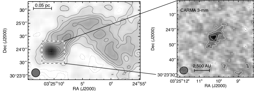
Figure 2.— Left panel shows the MAMBO 1.2 mm dust continuum emission, where there is both a compact central bright object ($S_{peak}=33~{}$m$\rm Jy\,beam^{-1}$) and also less bright and diffuse emission. Black solid contours represent [1, 2, 3, …, 15]$\times$2.5 m$\rm Jy\,beam^{-1}$ levels, and dashed contours are -2.5 and -5 m$\rm Jy\,beam^{-1}$ levels. The dashed rectangle shows the area imaged by CARMA data. Right panel shows the gray scale 3-mm continuum emission map observed with CARMA. Solid contours mark the [2, 3, 5]$\times$0.5 m$\rm Jy\,beam^{-1}$, while negative contours are shown by dotted lines. A faint central source is detected at the center of the image that matches the MAMBO peak position.

The MAMBO dust continuum emission map (left panel of Figure 2) can be decomposed into a bright compact core, and fainter filamentary emission. The compact core peak position is located at $(\alpha,\delta)=$(03:25:10.4, +30:23:56.0). The compact core within 4,200 AU mass is estimated to be 0.3 $M_{\odot}$, where a dust opacity per dust mass of 1.14 cm² g^-1 (Ossenkopf & Henning, 1994), gas-to-dust ratio of 100, and a dust temperature of 10 K are used. The MAMBO derived mass is consistent with the mass previously estimated using Bolocam. In Figure 3 the compact core is compared to the sample of starless cores from Kauffmann et al. (2008), where the fiducial radius of $4,200$ AU is used to compare with previous works (e.g., Motte & André, 2001). suggesting that it is more compact than most starless cores From this comparison we can establish that L1451-mm is in fact quite compact, and therefore dense, suggesting that it is more compact than most starless cores an evolved evolutionary state (see Crapsi et al., 2005).

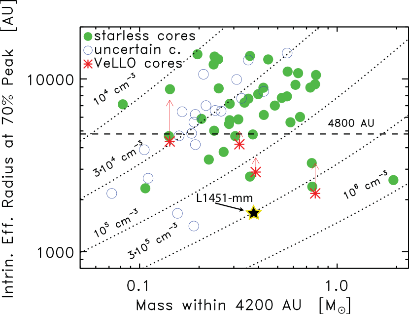
Figure 3.— Relation between the intrinsic radius at 70% peak intensity and the mass within 4200 AU radius from the peak for L1451-mm (show by the solid star), compared to the sample of starless cores and VeLLOs candidates from Kauffmann et al. (2008). Both properties (mass and radius) are derived from MAMBO data. Starless cores with well established and uncertain properties are shown by filled and open circles, respectively. Cores hosting candidate VeLLOs are shown by stars, the radius bias due to internal heating by the central object is indicated by the arrows (see Kauffmann et al., 2008, for details). Curves of constant $\rm H_{2}$ central density are shown by dotted lines. The dashed line indicates the upper radius limit for evolved dense cores, $\leq$4800 AU, suggested by Crapsi et al. (2005).

A faint central source is detected in the CARMA 3-mm continuum map shown in right panel of Figure 2. The continuum emission map is fitted by a Gaussian with a total flux of 10 mJy, while if a point source is fitted a flux of (4$\pm$2) mJy is obtained. A summary of the fits to the CARMA 3-mm continuum are listed in Table 7. The CARMA continuum emission agrees with the MAMBO peak position.

Table 7Results of Fits to CARMA 3-mm continuum image for L1451-mm

	Center		Peak Flux	Size (FWHM)	PA
Source	$\alpha$(J2000)	$\delta$(J2000)	(mJy)	(arcsec)	($\deg$)
Point Source	3:25:10.25	+30:23:55.09	4$\pm$2	$\cdots$	$\cdots$
Gaussian	3:25:10.21	+30:23:55.20	2$\pm$1	(16$\pm$13, 8$\pm$6)	$-$-37$\pm$44

4.2. Molecular lines with VLA and CARMA

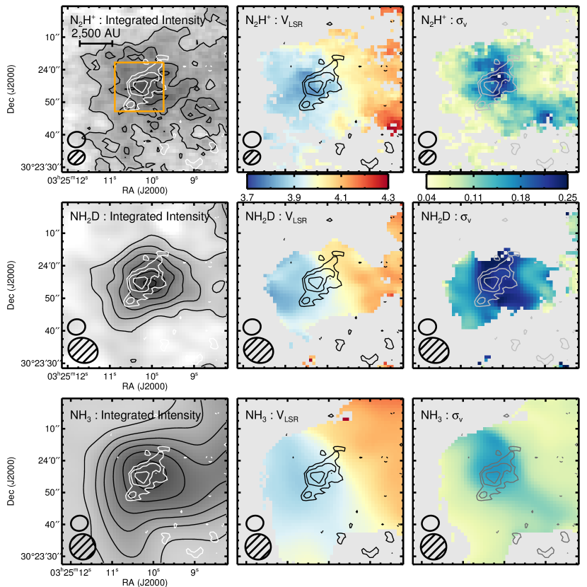
Figure 4.— Top, middle, and bottom rows present results from $\rm N_{2}H^{+}$ (CARMA), $\rm NH_{2}D$ (CARMA), and $\rm NH_{3}$ (VLA) emission line maps, respectively, where all observed hyperfine components are used. Left, middle, and right columns show the integrated intensity, centroid velocity, and velocity dispersion maps, respectively. Left panels also show contours for the integrated intensity at the following levels: [5,15,25] $\rm Jy\,beam^{-1}$ ${\rm km\,s^{-1}}$ for $\rm N_{2}H^{+}$ (top), [5,15,25,35,45,55] $\rm Jy\,beam^{-1}$ ${\rm km\,s^{-1}}$ for $\rm NH_{2}D$ (middle), [12.5,50,87.5,125,162.5,200] m$\rm Jy\,beam^{-1}$ ${\rm km\,s^{-1}}$ for $\rm NH_{3}$ (bottom). The color scales for the velocity (centroid and dispersion) maps are in ${\rm km\,s^{-1}}$. Contours show the CARMA 3-mm continuum emission presented in Figure 2. The synthesized beam for each transition line is shown at the bottom left corner and the CARMA 3-mm continuum beam shown above. The orange box in the upper left panel shows the region imaged using the SMA.

Figure 4 shows the summary of the molecular line transitions observed with CARMA and VLA. In this study we will briefly discuss the kinematics of the region and leave a more in depth study of the core in forthcoming papers (Schnee et al., 2011 in prep., Arce et al., 2011 in prep.). From these observations a centroid velocity and velocity dispersion are obtained by fitting the line profiles (see Rosolowsky et al., 2008, for details). The integrated intensity maps show the extended emission from the core where the peaks match the position of the CARMA continuum emission to within the respective beam size. The centroid velocity maps, for all three lines, show a consistent result with a clear velocity gradient. A gradient is fitted to the centroid velocity map for all three lines, with an average value of $\mathcal{G}=$6.1 km s^-1 pc^-1 and a $-66\arcdeg$ position angle (measured counter clockwise from north), see Table 8 for the individual fit obtained for all three maps. This velocity gradient is larger than those observed in lower angular resolution $\rm NH_{3}$ (1,1) maps (Goodman et al., 1993) or using lower density tracers (Kirk et al., 2010), while velocity gradients of a similar magnitude are obtained with high angular resolution observations of dense gas (Curtis & Richer, 2011; Tanner & Arce, 2011). The velocity dispersion maps show a clear increase towards the center of the map, starting with very narrow lines (close to the thermal values) in the outer regions. The increase in velocity dispersion is more pronounced in the $\rm N_{2}H^{+}$ velocity dispersion map, and the difference can be explained by the higher angular resolution obtained in the $\rm N_{2}H^{+}$ observations.

Table 8Velocity Gradients Fits

Transition	$\mathcal{G}$	PA	$v_{0}$
	(km s-1 pc-1)	(deg)	(${\rm km\,s^{-1}}$)
$\rm N_{2}H^{+}$	$5.6\pm 0.2$	$-84\pm 3$	$3.970\pm 0.002$
$\rm NH_{2}D$	$8\pm 1$	$-83\pm 15$	$3.949\pm 0.009$
$\rm NH_{3}$	$6.24\pm 0.06$	$-65.8\pm 0.7$	$4.0042\pm 0.0006$

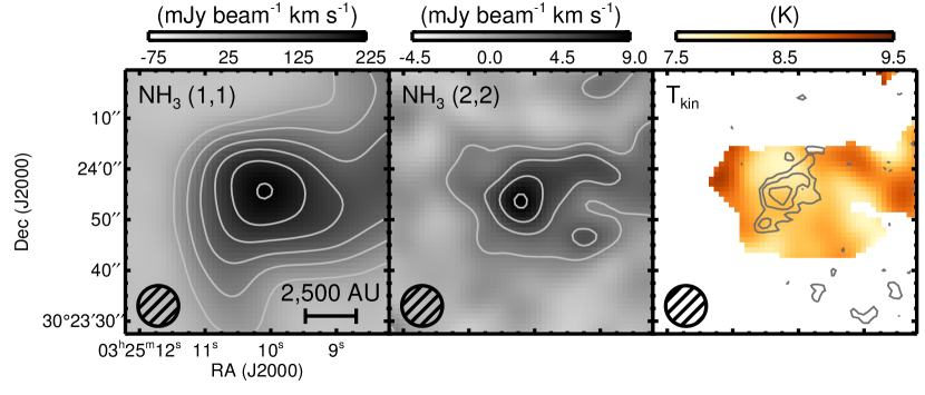
Figure 5.— Left and middle panels show the $\rm NH_{3}$ (1,1) and (2,2) integrated intensity VLA maps of the same region shown in Figure 4 using all the observed hyperfine components. The overlaid contours show the integrated intensity at [2,4,6,…,12] $\times$ 18.12 and 1.09 m$\rm Jy\,beam^{-1}$ ${\rm km\,s^{-1}}$ for $\rm NH_{3}$ (1,1) and (2,2) in the left and middle panels, respectively. The right panel shows the kinetic temperature derived by fitting simultaneously both $\rm NH_{3}$ lines, overlaid with the CARMA 3-mm continuum. The kinetic temperature uncertainties ranges between 0.2 K in the central region up to 0.5 K in the outer region. The kinetic temperature map presents small variations, where there is no increase in temperature at the peak position of the continuum emission.

The $\rm NH_{3}$ (1,1) and (2,2) integrated intensity maps obtained using the VLA are shown in Figure 5, left and middle panels respectively, where all components observed are taken into account. Both lines present a peak coincident with the CARMA continuum peak, and where the $\rm NH_{3}$ (1,1) emission covers a more extended region than the $\rm NH_{3}$ (2,2). However, since the emission $\rm NH_{3}$ (1,1) is fairly extended, the addition of GBT data to provide the zero-spacing is needed to allow a robust temperature determination. The morphology of the $\rm NH_{3}$ and $\rm N_{2}H^{+}$ integrated intensity maps show non-flattened structures, which are drastically different from those seen in young Class 0 sources (e.g., Wiseman et al., 2001; Chiang et al., 2010; Tanner & Arce, 2011). The right panel of Figure 5 presents the derived kinetic temperature obtained from the simultaneous $\rm NH_{3}$ (1,1) and (2,2) line fit, with uncertainties in the temperature determination between 0.2 K, in the central region, up to 0.5 K in the outer regions. Surprisingly, the kinetic temperature map is quite constant, in particular, there is no evidence for an increase in temperature towards the peak continuum position.

4.3. SMA

Figure 6.— Visibilities amplitude as a function of $uv$-distance. The dotted histogram indicates the expected amplitude in the absence of signal. The solid line shows the flux from the point source fit reported in Table 9.

Table 9Results of uv Fits of SMA 1.3-mm continuum data for L1451-mm

	Phase Center		Offset	Peak Flux	Size (FWHM)	PA
Source	$\alpha$(J2000)	$\delta$(J2000)	(arcsec)	(mJy)	(arcsec)	($\deg$)
Point Source (vis. longer than 40$k\lambda$)	3:25:10.21	+30:23:55.3	(0.40, $-$0.23)	27.0$\pm$0.4	$\cdots$	$\cdots$
Gaussian (all vis.)	$\cdots$	$\cdots$	(0.40, $-$0.23)	32.8$\pm$0.6	(0.66$\pm$0.05, 0.45$\pm$0.05)	-88$\pm$8

The visibility amplitude as a function of $uv$-distance for the 1.3-mm continuum is shown in Fig. 6. From this figure we identify two components. An extended component, that is resolved at long baselines, and a compact component that remains unresolved even at the longest baselines (indicated by the horizontal line in Figure 6). This unresolved component is commonly seen towards dense cores containing a central protostar, and it is interpreted as arising from an unresolved central disk (e.g., Jørgensen et al., 2007, 2009). However, in the case of L1451-mm there is no infrared detection of a central protostar.

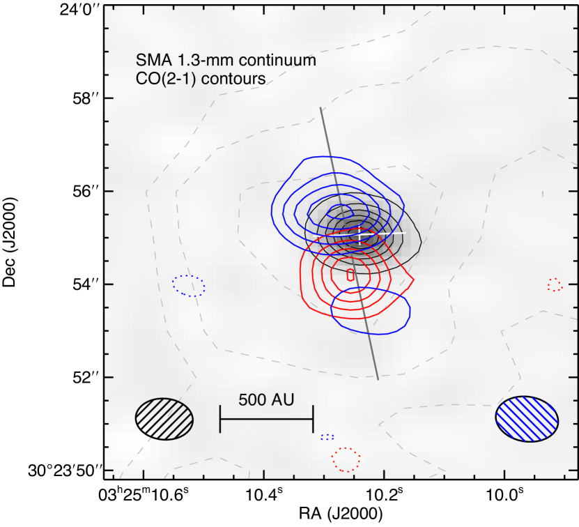
Figure 7.— The greyscale map shows the source detected in the 1.3-mm continuum continuum observed with SMA, with the overlaid black contours at [3,7,11,15,19,23] m$\rm Jy\,beam^{-1}$. Overlaid are the contours for the ${\rm{}^{12}CO}$ (2–1) integrated intensity using the red and blue channels (red and blue channels are taken between 5.3-6.9 ${\rm km\,s^{-1}}$ and 1.9-3.7 ${\rm km\,s^{-1}}$, respectively). Dotted contours denote negative contour levels. Contour levels are drawn at integer multiples of 114 m$\rm Jy\,beam^{-1}$  ${\rm km\,s^{-1}}$. Dashed light grey contours show the CARMA 3-mm continuum emission presented in Figure 2. The white line shows the direction of the Gaussian fit on the uv-plane as reported in Table 9. The gray line is cut for the position-velocity diagram shown in Figure 8. The 1.3-mm continuum ${\rm{}^{12}CO}$ (2–1) emission synthesized beams are shown at bottom left and right corners, respectively.

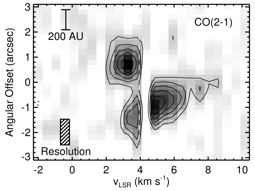
Figure 8.— Position velocity diagram for the SMA ${\rm{}^{12}CO}$ (2–1) data along the gray line shown in Figure 7. Contours drawn start at 0.3 $\rm Jy\,beam^{-1}$ with an increment of 0.24 $\rm Jy\,beam^{-1}$. The dashed vertical line shows the centroid velocity of the dense core, 3.94${\rm km\,s^{-1}}$.

The SMA 1.3-mm continuum map is shown in Figure 7, with red- and blue-shifted ${\rm{}^{12}CO}$ (2–1) emission overlaid. The dust continuum emission clearly shows the central source, also presented in Figure 6. The position of this continuum source coincides with the pixel where the CARMA 3-mm continuum peaks. The orientation of the SMA continuum emission, obtained through a fit of the visibilities and listed in Table 9, is close to the right ascension axis and clearly different from the red- and blue-shifted ${\rm{}^{12}CO}$ emission. The detected ${\rm{}^{12}CO}$ (2–1) emission shows a large velocity dispersion, with spatially separated blue- and red-shifted lobes (see Figure 7). Figure 8 shows the Position Velocity (PV) diagram along the gray line drawn in Figure 7, where the dashed vertical line shows the centroid velocity of the dense core, 3.94 ${\rm km\,s^{-1}}$, which is consistent with the interferometric observations (see Table 8) and the $\rm NH_{3}$ (1,1) data obtained with the GBT at 30$\arcsec$ (Pineda et al. 2011, in prep).

The dust mass of the compact (unresolved) emission is estimated as:

$$M_{1.3~{}mm}=1.3~{}{M_{\odot}}\left(\frac{F_{1.3~{}mm}}{1{\rm Jy}}\right)\left(\frac{d}{200~{}{\rm pc}}\right)^{2}\left(e^{0.36\,(30~{}K/T)}-1\right)~{},$$ (4)

where we assumed optically thin emission and a dust opacity per dust mass ($\kappa_{1.3~{}mm}$) of 0.86 cm² g^-1 (thick ice mantles coagulated at $10^{5}$ cm^-3 from Ossenkopf & Henning, 1994) and a gas-to-dust ratio of 100, see Jørgensen et al. (2007). The flux from the unresolved emission is estimated by fitting a point source to baselines longer than 40 $k\lambda$, as in Jørgensen et al. (2007), and therefore it avoids contamination from the dense core itself. The result of fitting a point source gives a flux of $27.0$ mJy, see Table 9, which implies a mass of

$$M_{1.3~{}mm}=0.024\,{M_{\odot}}$$ (5)

for a temperature of 30 K (as used in Jørgensen et al., 2007). This mass will be used as a first estimate for the circumstellar disk mass (see Jørgensen et al., 2007, for a discussion).

The disk–to–dense core mass ratio, $M_{disk}/M_{dense~{}core}$, is estimated using the disk mass from eq. 5 and the dense core mass. This ratio is low ($\approx$0.1) but comparable to Class 0 objects (Enoch et al., 2011; Jørgensen et al., 2009; Enoch et al., 2009a).

4.4. Simultaneous Fit of Visibilities and Broadband SED

A powerful way to constrain the physical parameters of dense cores and YSOs is by fitting the broadband SED (e.g., Robitaille et al., 2007). In the case of L1451-mm, only detections at 160 and 1200 $\mu$m are available, which makes the broadband SED fit a not well-constrained problem. Here, the information from the 1.3-mm continuum observations (SMA) is extremely important to help discriminate between different physical models (e.g., Enoch et al., 2009a).

In order to compare the continuum emission model with the interferometric observations, the model is sampled in uv-space to match the observations using the uvmodel task in MIRIAD. The synthetic and observed visibilities are both binned in uv-distance (using the uvamp task in MIRIAD), and then they are added as an extra term to the $\chi^{2}$ to minimize,

$$\chi^{2}_{vis}=\sum_{i}\left(\frac{V_{i,obs}-V_{i,model}}{\sigma_{V_{i,obs}}}\right)^{2},$$ (6)

where $V_{i,obs}$ and $V_{i,model}$ are the average observed and synthetic visibilities in the $i$ bin, respectively, while $\sigma_{V_{i,obs}}$ is the uncertainty of the observed average visibility. The $\chi^{2}$ subject to minimization is

$$\chi^{2}=(1-Q)\chi^{2}_{SED}+Q\chi^{2}_{vis},$$ (7)

where $Q$ is an ad-hoc weight used to control how important it is to fit the visibilities compared to the broadband SED. In this case a $Q=0.5$ is used, which gives the same weight to the SED and visibilities fit.

Because of the problem’s high dimensionality, the $\chi^{2}$ minimization is carried out with a genetic algorithm (Johnston et al., 2011), while the model SEDs and visibilities are calculated with a new Monte-Carlo radiation transfer code (Robitaille et al., 2011 in prep), which is based on the radiative transfer code presented by Whitney et al. (2003b). The new code uses raytracing for the thermal emission at sub-mm and mm wavelengths, providing excellent signal-to-noise to fit the long-wavelength SED and visibilities.

Using this fitting program we explore three models with increasing levels of complexity to explain our observations: a) starless isothermal dense core; b) dense core with a YSO and disk at the center; and c) dense core with a central FHSC.

The parameter ranges searched using the genetic algorithm is given in Table 10, a summary of the fit results is shown in Figure 9, and the model parameters are listed in Table 11.

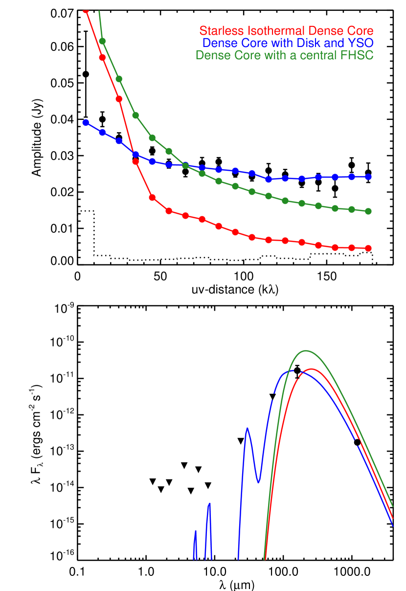
Figure 9.— Summary of best-fit of the broadband SED and dust continuum visibilities for three different models: starless isothermal dense core in red; dense core with a YSO and disk at the center in blue; and dense core with a central FHSC in green. The data are shown in black. The top panel shows the visibilities in filled circles. The bottom panel shows the broadband SED for L1451-mm, where the upper limits are shown by triangles, measurements are shown by filled black circles, and the best model fits are shown by the solid curves.

Table 10Parameter Ranges Searched

Parameter	Description	Value/Range	Sampling
Starless Dense Core
$p$	Exponent of density profile	$-2$ – $0$	linear
$M_{dense~{}core}$	Envelope Mass ($M_{\odot}$)	$10^{-5}$ – $10$	logarithmic
$T_{dust}$	Envelope temperature (K)	$5$ – $30$	linear
$R_{max}$	Envelope outer radius (AU)	$1,000$ – $5,000$	logarithmic
Dense Core with Disk and YSO
$L_{int}$	Intrinsic luminosity ($L_{\odot}$)	$10^{-4}$ – $0.1$	logarithmic
$\dot{M}_{infall}$	Infall rate ($M_{\odot}\,{\rm yr^{-1}}$)	$10^{-9}$ – $10^{-6}$	logarithmic
$R_{env}$	Outer envelope radius (AU)	$1,000$ – $5,000$	logarithmic
$R_{cent}$	centrifugal radius (AU)	$50$ – $1,000$	logarithmic
$R_{disk}$	outer disk radius (AU)	$50$ – $1,000$	logarithmic
$M_{disk}$	Disk Mass ($M_{\odot}$)	$10^{-8}$ – $10^{-3}$	logarithmic
$i$	Viewing Angle ($\deg$)	$0$ – $90$	linear

Starless isothermal dense core

The simplest model consist of a pure isothermal dense core with a density profile $n\propto r^{-p},$ where the exponent, $p$, of the density profile is a free parameter, but constrained to values smaller than $2$. The dense core temperature, $T_{dust}$, and the outer radius, $R_{env}$, are also parameters in the fit, which are listed in Table 11 along with the dense core mass, $M_{env}$. The best model fit for the starless isothermal dense core model is shown in red in Figure 9, where it shows that this model does not provide a good match to the visibilities. If the power-law density exponent is not constrained, then a very steep density profile, $n\propto r^{-2.8}$, can actually match both the SED and visibilities. However, a power-law exponent of $-2.8$ is beyond the range deemed physically reasonable. Because, even though the outer region of starless cores (and cylindrical filaments) can have similar steep density profiles (e.g., Tafalla et al., 2002), in the inner region ($r<$3,000 AU) their density profiles are flat, which is exactly the region we are interested in to produce the compact emission.

Dense Core with a central YSO and disk

The next model fitted is one composed of a dense core with a central YSO and disk. The dense core is modelled as a rotating and infalling envelope (Ulrich, 1976), with outer radius $R_{\rm env}$, total mass $M_{\rm env}$, and infall rate $\dot{M}_{\rm infall}$. The density of the envelope is given in spherical polar coordinates by

$$\rho(r,\theta,\phi)=\rho_{0}^{\rm env}\left(\frac{r}{R_{\rm c}}\right)^{-3/2}\left(1+\frac{\mu}{\mu_{0}}\right)^{-1/2}\left(\frac{\mu}{\mu_{0}}+\frac{2\mu_{0}^{2}R_{\rm c}}{r}\right)^{-1}$$ (8)

where $R_{\rm c}$ is the centrifugal radius, $\mu=\cos{\theta}$, and $\mu_{0}$ is the cosine of the polar angle of a streamline of infalling particles as $r\rightarrow\infty$, which is given by:

$$\mu_{0}^{3}+\mu_{0}\left(\frac{r}{R_{\rm c}}-1\right)-\mu\left(\frac{r}{R_{\rm c}}\right)=0$$ (9)

The normalization constant $\rho_{0}^{\rm env}$ is related to the infall rate by:

$$\rho_{0}^{\rm env}=\frac{\dot{M}_{\rm infall}}{4\pi\left(GM_{*}R_{\rm c}^{3}\right)^{1/2}}~{},$$ (10)

where $M_{*}$ is the mass of the central object. The disk is modeled as a passive flared disk described in cylindrical polar coordinates by

$$\rho(R,z,\phi)=\rho_{0}^{\rm disk}\,\left(\frac{100\,AU}{R}\right)^{\beta-q}\,\exp{\left[-\frac{1}{2}\left(\frac{z}{h(R)}\right)^{2}\right]}$$ (11)

where $\rho_{0}^{\rm disk}$ is defined by the disk mass $M_{\rm disk}$, $q$ is the surface density radial exponent (which we set to $-1$), $\beta$ is the disk flaring power (set to $1.25$), and the disk scale-height $h(R)$ is given by:

$$h(R)=h_{0}\,\left(\frac{R}{100\,AU}\right)^{\beta}.$$ (12)

where $h_{0}$ is the scale-height at 100 AU and it is set to 10 AU.

The viewing angle $i$ is a parameter in the fitting. The central protostar is modeled as an object with an effective surface temperature of 3,000 K and intrinsic luminosity $L_{int}$, where the parameter $L_{int}$ includes the luminosity due to accretion.

The temperature is computed self-consistently with the density using the radiation transfer code, see Whitney et al. (2003b, a, 2004). It assumes a geometry (e.g., Ulrich envelope model with a flared disk), the dust properties, and local thermodynamic equilibrium. Here we use dust opacities of Ossenkopf & Henning (1994) for dust grains with thick ice mantles after $10^{5}$ years of coagulation at a density of $10^{6}$ cm^-3.

The best model parameters are listed in Table 11. This model provides an excellent fit to the visibilities, while the SED fit underestimates the flux at $160\mu m$.

Table 11Best Model Fit Parameters

Model	$L_{int}$	$\dot{M}_{infall}$	$M_{disk}$	$R_{disk}$	Viewing Angle	$M_{dense~{}core}$	$R_{env}$	$T_{dust}$
	($L_{\odot}$)	($M_{\odot}\,{\rm yr^{-1}}$)	($M_{\odot}$)	(AU)	($\deg$)	($M_{\odot}$)	(AU)	(K)
Starless Dense Core	$\cdots$	$\cdots$	$\cdots$	$\cdots$	$\cdots$	$0.353$	$1001$	$10.2$
Dense Core with Disk and YSO	$0.0450$	$7.1\times 10^{-6}$	$0.086$	$107$	$64.9$	$0.146$	$1007$	$\cdots$
Dense Core with central FHSC	$\cdots$	$\cdots$	$\cdots$	$\cdots$	$\cdots$	$0.56$	$2543$	$\cdots$

Given the best fit result we estimate the accretion luminosity, $L_{acc}$, as

$$L_{acc}=\frac{G\,M_{*}\,\dot{M}_{acc}}{R_{*}}~{},$$ (13)

where $M_{*}$ and $R_{*}$ are the protostellar mass and radius, and $\dot{M}_{acc}$ is the accretion rate onto the protostar. Using equation (13) we obtain an accretion luminosity of $6\,{L_{\odot}}$, where we have assumed that the accretion rate is the same as the infall rate,

$$\dot{M}_{acc}=\dot{M}_{infall}=2.4\times 10^{-5}\,\left(\frac{M_{*}}{{M_{\odot}}}\right)^{0.5}{M_{\odot}\,{\rm yr^{-1}}},$$ (14)

the minimum mass of the central object is the mass of the disk, $M_{*}=M_{disk}=0.086\,{M_{\odot}}$, and that the central object might be a young protostar, $R_{*}=3\,{R_{\odot}}$. This expected accretion luminosity is $100$ times higher than what can be kept hidden at the center of the core in the best-fit model, and therefore some of the assumptions must be clearly misrepresenting reality. Another simple estimate that is derived from equation (13) is the accretion rate onto the central object needed to produce the same luminosity of the best model, obtaining $\dot{M}_{acc}=2.45\times 10^{-8}\,{M_{\odot}\,{\rm yr^{-1}}}$ (much lower than the estimated infall rate, $7.1\times 10^{-6}\,{M_{\odot}\,{\rm yr^{-1}}}$). Clearly, in order to make a self-consistent model an extremely low accretion rate must be assumed.

Dense Core with a central FHSC

Another possibility to reconcile the low luminosity observed and the accretion rates expected from the models presented above is to increase the stellar radius, $R_{*}$. There is one object which has been predicted from numerical simulations (Larson, 1969; Masunaga et al., 1998; Masunaga & Inutsuka, 2000; Machida et al., 2008) that is large enough to fit the description: the first hydrostatic core (FHSC).

Masunaga et al. (1998) performed radiation hydrodynamic simulations of a collapsing core until the formation of a FHSC and found that for an initial core of 0.3 $M_{\odot}$ (model M3a), a FHSC of $R_{*}\sim 5\,$AU and $L_{int}\approx 0.03\,{L_{\odot}}$ (including accretion luminosity) is formed. We use the density and temperature profile resulting from this simulation as the input parameter for the radiative transfer code. The mass and radius of the dense core are varied (see Table 11) to find the best match of the observed SED and visibilities, see green points in Figure 9. Notice that this model does not use the same density and temperature profile as used in the dense core with disk and YSO model, and this explains the different SEDs. It is clear that the FHSC model visibilities do not provide as good a match to the observations as the YSO model, however, the FHSC model only have two free parameters compared to the seven free parameters of the YSO model.

4.5. The nature of the ${\rm{}^{12}CO}$ (2–1) emission

If there is no source of heating within the core, then ${\rm{}^{12}CO}$ should freeze-out onto dust grains (e.g., Tafalla et al., 2002). Therefore, the presence of the ${\rm{}^{12}CO}$ (2–1) emission in itself is strongly suggestive of a central heating source. From the $\rm NH_{3}$, $\rm N_{2}H^{+}$ and $\rm NH_{2}D$ centroid velocity maps it is clear that the velocity gradient is in the RA direction while the ${\rm{}^{12}CO}$ emission is more or less perpendicular. Since the orientation of the dust continuum emission detected with SMA is almost perpendicular to the ${\rm{}^{12}CO}$ (2–1) emission, we argue in favor of a central object and outflow system.

The amount of mass needed to keep material at 560 AU with a velocity of 1.3 ${\rm km\,s^{-1}}$ (similar parameters to the ${\rm{}^{12}CO}$ emission) is $\approx 0.53\,{M_{\odot}}$, which is almost twice the total mass in the dense core. Therefore, despite the low velocity seen in the ${\rm{}^{12}CO}$ (2-1) emission this gas is unbound and it is consistent with ${\rm{}^{12}CO}$ (2–1) tracing a slow molecular outflow.

4.6. Outflow Properties

The physical parameters of molecular outflows are typically calculated using both ${\rm{}^{12}CO}$ and ${\rm{}^{13}CO}$ lines (e.g., Arce et al., 2010). Unfortunately, in L1451-mm there are no detections of ${\rm{}^{13}CO}$ (2–1) and we are left to use only the ${\rm{}^{12}CO}$ (2–1) emission to study the high-velocity gas.

A lower limit for the mass entrained by the outflow, $M_{flow}$, is estimated assuming that the ${\rm{}^{12}CO}$ (2–1) emission is optically thin (see details in Appendix A) and with an excitation temperature of $T_{ex}=20$ K. The momentum ($P_{flow}$) and energy ($E_{flow}$) of the outflow along the line of sight are estimated following Cabrit & Bertout (1990),

$$P_{flow} = \sum_{i}M_{out,i}\,|v_{i}-v_{center}|~{},$$ (15)

$$E_{flow} = \frac{1}{2}\sum_{i}M_{out,i}\,|v_{i}-v_{center}|^{2}~{},$$ (16)

where $M_{out,i}$ is the mass in voxel $i$, $v_{center}$ is the velocity of the core, and $v_{i}$ is the velocity of voxel $i$. Also, the outflow characteristic velocity, $v_{flow}$, is calculated as $P_{flow}/M_{flow}$. An upper limit for the lobe size, $R_{lobe}$, is estimated from the (not deconvolved) extension of the red- and blue-shifted ${\rm{}^{12}CO}$ emission ($2\,R_{lobe}$) $\approx 4.5\arcsec$, or $\approx 1,120$ AU at the distance of Perseus. We also calculate the dynamical time, $\tau_{dyn}=R_{lobe}/v_{flow}$, mechanical luminosity, $L_{flow}=E_{flow}/\tau_{dyn}$, force, $F_{flow}=P_{flow}/\tau_{dyn}$, and rate, $\dot{M}_{flow}=M_{flow}/\tau_{dyn}$.

The outflow properties are calculated using only the voxels with signal-to-noise ratio higher than $2$. To avoid contamination in the outflow parameters from the cloud emission the central channel is not used in the calculations, and a second estimate is calculated where the three central channels are removed. The outflow parameters are reported in Table 12, where we notice that the differences between the quantities calculated using both methods are small.

The outflow properties presented in Table 12 show an extremely weak outflow in L1451-mm. However, when compared to the outflow found towards L1014 by Bourke et al. (2005) both $P_{flow}$ and $E_{flow}$ are close to the lower limits estimated using similar assumptions.

Table 12Summary of Outflow Properties

Property
Mass ($M_{\odot}$)	$1.2\times 10^{-5}$ ($8.4\times 10^{-6}$)
Momentum ($M_{\odot}$ ${\rm km\,s^{-1}}$)	$1.7\times 10^{-5}$ ($1.4\times 10^{-5}$)
Energy (ergs)	$3.1\times 10^{38}$ ($3.0\times 10^{38}$)
Luminosity ($L_{\odot}$)	$1.3\times 10^{-6}$ ($1.6\times 10^{-6}$)
Force ($M_{\odot}$ ${\rm km\,s^{-1}}$ yr-1)	$8.3\times 10^{-9}$ ($9.3\times 10^{-9}$)
Characteristic Velocity (${\rm km\,s^{-1}}$)	$1.3$ ($1.7$)
Dynamical Time (yr)	$2.0\times 10^{3}$ ($1.6\times 10^{3}$)
Outflow rate ($M_{\odot}\,{\rm yr^{-1}}$)	$6\times 10^{-9}$ ($5\times 10^{-9}$)

Note. — Properties are calculated without the central channel, while the values in parentheses are calculated without the 3 central channels.

The dynamical time is consistent with the FHSC estimated lifetime (e.g., Machida et al., 2008).

Recent three-dimensional radiation magneto hydrodynamics (RMHD) simulations of the dense core collapse (Machida et al., 2008; Tomida et al., 2010b; Commerçon et al., 2010) show that when the FHSC is formed a slow outflow can be driven even before the existence of a protostar (see also Tomisaka, 2002; Banerjee & Pudritz, 2006). In these simulations, the outflow that is generated is poorly collimated and typically has maximum velocity of 3 ${\rm km\,s^{-1}}$– very similar to the observed outflow in L1451-mm. In contrast, theoretical models (Shang et al., 2007; Pudritz et al., 2007) and observations (e.g., Arce et al., 2007) indicate that outflows from young protostars are highly collimated and exhibit velocities of a few tens of ${\rm km\,s^{-1}}$ although outflows from VeLLOs display lower velocities (André et al., 1999; Bourke et al., 2005).

The properties of the L1451-mm molecular outflow are consistent with a picture where a first hydrostatic core is the driving source of the poorly collimated and slow outflow observed.

5. Discussion

The detection of an unresolved source of continuum in the CARMA and SMA observations strongly suggests the presence of a central source of radiation and/or a disk. Moreover, the simultaneous fit of the broadband SED and the continuum visibilities rules out the possibility of explaining the observations without a central source (either a YSO or a FHSC). From the SED modeling it appears feasible to hide the central YSO even at 70$\mu$m, but it also requires an extremely inefficient or episodic accretion process. This might be consistent with the results obtained by Enoch et al. (2009b); Dunham et al. (2010) and Offner & McKee (2011), where episodic accretion is argued to explain the low luminosity of YSOs observed by Spitzer.

If the unresolved emission observed with the SMA is interpreted as a disk (as done by Jørgensen et al., 2007), then the disk mass is already $\sim$10% of the dense core mass, which is similar to the disk mass found in class 0 objects (e.g., Enoch et al., 2011, 2009a; Maury et al., 2010), although Belloche et al. (2002) shows evidence for a small disk in the young protostar IRAM 04191 ($M_{disk}<10^{-3}{M_{\odot}}$ and $M_{core}\approx 1.5\,{M_{\odot}}$). These studies of Class 0 objects suggests that the assembly of mass to form a disk starts very early on.

A slow molecular outflow is detected in the ${\rm{}^{12}CO}$ (2–1) line, see Sec. 4.5 and 4.6. Its orientation is almost perpendicular to the velocity gradient seen in dense gas tracers observed with VLA and CARMA ($\rm NH_{3}$, $\rm N_{2}H^{+}$ and $\rm NH_{2}D$), and despite the low velocity the gas is unbound. The properties presented in Table 12 place it as the weakest outflow found so far, with the lowest energy and momentum measured. Unfortunately, we have no estimate of the outflow inclination angle and therefore some of the outflow parameters might be underestimated. If the outflow is close to the plane of the sky, then the outflow velocity would be faster but it still could be consistent with a slow outflow driven by a FHSC depending on how large is the correction. This, however, would imply that the outflow extension is the one measured in the data, and therefore the outflow would have a shorter dynamical time and low degree of collimation. On the other hand, if the outflow is nearly in the line-of-sight, then the outflow velocity is similar to the 1.5 ${\rm km\,s^{-1}}$ measured from the data. However, the outflow extension would be much larger implying a longer dynamical time, which might be similar to those predicted by Tomida et al. (2010a) for FHSCs in recent numerical simulations. Therefore, constraining the inclination angle (e.g., through observations of the outflow cavity as in Huard et al., 2006) would provide important insight regarding the outflow and by extension to the central object.

For all the reasons listed above, we claim that a central source of radiation (either a YSO or a FHSC) must be present within L1451-mm. The lack of sensitive observations at mid-infrared wavelengths restricts our ability to carry out a more detailed modeling of this object. From our best-fit models we predict that L1451-mm should be detected by the Herschel Gould Belt Survey (André & Saraceno, 2005), similar to the observations by Linz et al. (2010). Therefore, those observations will provide a definitive answer regarding the luminosity of the central source and give more constraints to the modeling.

One way to explain our observations is by having a first hydrostatic core at the center of the dense L1451-mm core, instead of a YSO. The simultaneous fit of both visibilities and broadband SED shows that a FHSC can also provide a good fit to the observations, with the advantage of having an accretion luminosity consistent with the observations. The presence of a slow and poorly collimated outflow further supports this scenario. It is for these reasons that we propose L1451-mm to be a FHSC candidate.

Future observations of L1451-mm with interferometers using a more extended configuration and/or different frequencies will probe the currently unresolved continuum emission. We expect that such observations will provide a constraint on the origin of the emission (i.e., disk or first hydrostatic core). And, if the disk is confirmed, then a comparison with more evolved disks can be carried out. Moreover, observations of ${\rm{}^{12}CO}$ (3–2) would provide an estimate of the gas temperature, and therefore a good test to confirm that the ${\rm{}^{12}CO}$ emission is generated by an outflow (where the gas is usually warm).

It is very important to note that three out of the four known FHSC candidates are found in the same molecular cloud (Enoch et al., 2010; Chen et al., 2010). We compare this number to the expected number of FHSC in Perseus assuming a constant star formation rate, which can be estimated as

$$N_{FHSC}=N_{Class~{}0}\frac{\tau_{FHSC}}{\tau_{Class~{}0}}~{}.$$ (17)

We estimate the FHSC lifetime to be $\sim 10^{3}$ yr (e.g., Machida et al., 2008), the number of Class 0 sources in Perseus is $20-35$ (Hatchell et al., 2007; Enoch et al., 2009b), and the Class 0 lifetime is $2-5\times 10^{5}$ yr (Visser et al., 2001; Hatchell et al., 2007; Enoch et al., 2009b). Finally, the expected number of FHSC in Perseus is $\leq 0.2$ objects (similar results are obtained using statistics for Class I objects, e.g., Evans et al., 2009), and therefore, if all three candidates are confirmed, either Perseus is in an extremely peculiar epoch (e.g., a recent burst on the star formation rate) or this stage is longer than previously predicted by numerical simulations. A longer lifetime for the FHSC stage, up to $10^{4}$ yrs, has recently been suggested by Tomida et al. (2010a) for FHSCs formed in low-mass dense cores ($\sim 0.1$ $M_{\odot}$).

6. Summary

We present IRAM 30-m, CARMA, VLA, and SMA observations of the isolated low-mass dense core L1451-mm in the Perseus Molecular Cloud. No point source is detected towards the center of the core in NIR and Spitzer observations; however, a dust continuum source is identified in both CARMA and SMA continuum maps. Upper limits on the bolometric luminosity and temperature, $L_{bol}$ and $T_{bol}$, of 0.05 $L_{\odot}$ and $30$ K are estimated. Also, ${\rm{}^{12}CO}$ (2–1) emission is observed towards L1451-mm suggestive of a slow and poorly collimated outflow. Modeling the broadband SED and observed visibilities at 1.3-mm confirms the need for a YSO or a First Hydrostatic Core (FHSC) to explain the observations. However, more high-resolution observations are needed to distinguish between these two scenarios.

Although YSO and FHSC models are almost indistinguishable, the FHSC scenario seems more likely from the data at hand (and thus we may call L1451-mm a FHSC candidate).

Finally, if all current FHSC candidates are confirmed, then an important revision of the FHSC lifetime must be carried out, which may include modifications of the numerical simulations (e.g., Tomida et al., 2010a).

Appendix A Calculation of CO column density

If the levels of the molecule are populated following a Boltzmann distribution of temperature $T_{ex}$, then the column density can be expressed as,

$$N_{J} = \frac{8\pi\nu^{3}}{c^{3}}\frac{g_{J}}{g_{J+1}}\frac{1}{A_{J+1\rightarrow J}}\frac{\int\tau\,dv}{\left(1-e^{-h\nu/kT_{ex}}\right)}$$

$$N_{J} = 93.28\left(\frac{2J+1}{2J+3}\right)\frac{\nu^{3}}{A_{J+1\rightarrow J}}\frac{\int\tau\,dv}{\left(1-e^{-T_{0}/T_{ex}}\right)}\,$$ (A1)

where $g_{J}=(2J+1)$ is the statistical weight of level $J$ for a linear rotor molecule, $\nu$ is the transition frequency in units of GHz, $A_{J+1\rightarrow J}$ is the spontaneous emission coefficient in s^-1, $\tau$ is the transition optical depth, the velocity is in ${\rm km\,s^{-1}}$, and

$$T_{0}\equiv\frac{h\,\nu}{k}\,.$$ (A2)

In the case of ${\rm{}^{12}CO}$ (2–1), we use $\nu=230.538\,{\rm GHz}$ and $A_{2\rightarrow 1}=6.91\times 10^{-7}\,{\rm s}^{-1}$ (obtained from Leiden Atomic and Molecular Database), and therefore $T_{0}=11.0641~{}{\rm K}$.

Using the equation of radiative transfer to relate the observed emission, $T_{R}$, with excitation temperature, $T_{ex}$, and background temperature, $T_{cmb}$, we obtain:

$$T_{R} = T_{0}\left[\frac{1}{(e^{T_{0}/T_{ex}}-1)}-\frac{1}{(e^{T_{0}/T_{cmb}}-1)}\right]\left(1-e^{-\tau}\right)$$

$$\int T_{R}\,dv = T_{0}\left[\left(e^{T_{0}/T_{ex}}-1\right)^{-1}-\left(e^{T_{0}/T_{cmb}}-1\right)^{-1}\right]\int\tau\,dv~{},$$ (A3)

where optically thin emission is assumed.

Combining equations (A1) and (A3), the column density of the level $J$ can be calculated as,

$$N_{J} = 93.28\left(\frac{2J+1}{2J+3}\right)\frac{\nu^{3}}{A_{J+1\rightarrow J}}\frac{\int T_{MB}\,dv}{\left(1-e^{-T_{0}/T_{ex}}\right)T_{0}\left[\left(e^{T_{0}/T_{ex}}-1\right)^{-1}-\left(e^{T_{0}/T_{cmb}}-1\right)^{-1}\right]}$$

$$N_{1}({{\rm{}^{12}CO}}) = 9.924\times 10^{14}\frac{\int T_{MB}\,dv}{\left(1-e^{-11.06/T_{ex}}\right)11.06\left[\left(e^{11.06/T_{ex}}-1\right)^{-1}-\left(e^{11.06/T_{cmb}}-1\right)^{-1}\right]}\ {\rm cm^{-2}},$$ (A4)

where equation (A4) gives the column density of the level $J=1$ of ${\rm{}^{12}CO}$ using the ${\rm{}^{12}CO}$ (2–1) transition emission.

The total column density of ${\rm{}^{12}CO}$ is calculated as

$$N({{\rm{}^{12}CO}})=\frac{Z}{g_{J}e^{-E_{J}/k\,T_{ex}}}N_{J}({{\rm{}^{12}CO}})=\frac{Z}{(2J+1)}e^{J(J+1)B\,h/k\,T_{ex}}N_{J}({{\rm{}^{12}CO}})~{},$$ (A5)

where $B$ is the rotation constant for a linear rotor ($B=57.635968$ GHz for ${\rm{}^{12}CO}$), and $Z$ is the partition function, which can be approximated as $Z\approx k\,T_{ex}/(h\,B)$. Therefore, in the case of ${\rm{}^{12}CO}$ $J=1$ we obtain,

$$N({{\rm{}^{12}CO}})=1.2\times 10^{14}\,\frac{T_{ex}/11.06}{\left(e^{11.06/T_{ex}}-1\right)^{-1}-\left(e^{11.06/T_{cmb}}-1\right)^{-1}}\frac{e^{5.53/T_{ex}}\,\int T_{MB}\,dv}{\left(1-e^{-11.06/T_{ex}}\right)}\ {\rm cm^{-2}},$$ (A6)

which when combined with a ${\rm{}^{12}CO}$ abundance with respect to $\rm H_{2}$, $[{{\rm{}^{12}CO}}/{\rm H_{2}}]=10^{-4}$, provides an estimate of the total column density of $\rm H_{2}$.

The final conversion between column density and mass is done using

$$M=2.71\times 10^{-8}\left(\frac{N({{\rm{}^{12}CO}})}{10^{14}\,{\rm cm^{-2}}}\right)\left(\frac{[{\rm H_{2}}/{{\rm{}^{12}CO}}]}{10^{4}}\right)\left(\frac{d}{250\,{\rm pc}}\right)^{2}\left(\frac{A_{sky}}{\rm arcsec^{2}}\right)\left(\frac{\mu}{2.3}\right){M_{\odot}}\,,$$ (A7)

where $A_{sky}$ is the area on the sky used to calculate $N({{\rm{}^{12}CO}})$, and $\mu$ is the mean molecular weight.

References

- André et al. (1999) André, P., Motte, F., & Bacmann, A. 1999, ApJ, 513, L57
- André & Saraceno (2005) André, P., & Saraceno, P. 2005, in ESA Special Publication, Vol. 577, ESA Special Publication, ed. A. Wilson, 179–184
- Arce et al. (2010) Arce, H. G., Borkin, M. A., Goodman, A. A., Pineda, J. E., & Halle, M. W. 2010, ApJ, 715, 1170
- Arce et al. (2007) Arce, H. G., Shepherd, D., Gueth, F., Lee, C.-F., Bachiller, R., Rosen, A., & Beuther, H. 2007, in Protostars and Planets V, ed. B. Reipurth, D. Jewitt, & K. Keil, 245–260
- Banerjee & Pudritz (2006) Banerjee, R., & Pudritz, R. E. 2006, ApJ, 641, 949
- Belloche et al. (2002) Belloche, A., André, P., Despois, D., & Blinder, S. 2002, A&A, 393, 927
- Belloche et al. (2006) Belloche, A., Parise, B., van der Tak, F. F. S., Schilke, P., Leurini, S., Güsten, R., & Nyman, L. 2006, A&A, 454, L51
- Belloche et al. (2011) Belloche, A., et al. 2011, A&A, 527, A145+
- Bertin & Arnouts (1996) Bertin, E., & Arnouts, S. 1996, A&AS, 117, 393
- Bourke et al. (2005) Bourke, T. L., Crapsi, A., Myers, P. C., Evans, II, N. J., Wilner, D. J., Huard, T. L., Jørgensen, J. K., & Young, C. H. 2005, ApJ, 633, L129
- Cabrit & Bertout (1990) Cabrit, S., & Bertout, C. 1990, ApJ, 348, 530
- Caselli et al. (2002) Caselli, P., Benson, P. J., Myers, P. C., & Tafalla, M. 2002, ApJ, 572, 238
- Cernis (1990) Cernis, K. 1990, Ap&SS, 166, 315
- Chen et al. (2010) Chen, X., Arce, H. G., Zhang, Q., Bourke, T. L., Launhardt, R., Schmalzl, M., & Henning, T. 2010, ApJ, 715, 1344
- Chiang et al. (2010) Chiang, H., Looney, L. W., Tobin, J. J., & Hartmann, L. 2010, ApJ, 709, 470
- Commerçon et al. (2010) Commerçon, B., Hennebelle, P., Audit, E., Chabrier, G., & Teyssier, R. 2010, A&A, 510, L3+
- Corder et al. (2010) Corder, S. A., Wright, M. C. H., & Carpenter, J. M. 2010, in Society of Photo-Optical Instrumentation Engineers (SPIE) Conference Series, Vol. 7733, Society of Photo-Optical Instrumentation Engineers (SPIE) Conference Series
- Crapsi et al. (2005) Crapsi, A., Caselli, P., Walmsley, C. M., Myers, P. C., Tafalla, M., Lee, C. W., & Bourke, T. L. 2005, ApJ, 619, 379
- Curtis & Richer (2011) Curtis, E. I., & Richer, J. S. 2011, MNRAS, 410, 75
- di Francesco et al. (2007) di Francesco, J., Evans, II, N. J., Caselli, P., Myers, P. C., Shirley, Y., Aikawa, Y., & Tafalla, M. 2007, in Protostars and Planets V, ed. B. Reipurth, D. Jewitt, & K. Keil, 17–32
- Dunham et al. (2008) Dunham, M. M., Crapsi, A., Evans, II, N. J., Bourke, T. L., Huard, T. L., Myers, P. C., & Kauffmann, J. 2008, ApJS, 179, 249
- Dunham et al. (2010) Dunham, M. M., Evans, N. J., Terebey, S., Dullemond, C. P., & Young, C. H. 2010, ApJ, 710, 470
- Dunham et al. (2006) Dunham, M. M., et al. 2006, ApJ, 651, 945
- Enoch et al. (2009a) Enoch, M. L., Corder, S., Dunham, M. M., & Duchêne, G. 2009a, ApJ, 707, 103
- Enoch et al. (2009b) Enoch, M. L., Evans, N. J., Sargent, A. I., & Glenn, J. 2009b, ApJ, 692, 973
- Enoch et al. (2008) Enoch, M. L., Evans, II, N. J., Sargent, A. I., Glenn, J., Rosolowsky, E., & Myers, P. 2008, ApJ, 684, 1240
- Enoch et al. (2010) Enoch, M. L., Lee, J., Harvey, P., Dunham, M. M., & Schnee, S. 2010, ApJ, 722, L33
- Enoch et al. (2006) Enoch, M. L., et al. 2006, ApJ, 638, 293
- Enoch et al. (2011) —. 2011, ApJS, 195, 21
- Evans et al. (2009) Evans, N. J., et al. 2009, ApJS, 181, 321
- Foster & Goodman (2006) Foster, J. B., & Goodman, A. A. 2006, ApJ, 636, L105
- Goodman et al. (1998) Goodman, A. A., Barranco, J. A., Wilner, D. J., & Heyer, M. H. 1998, ApJ, 504, 223
- Goodman et al. (1993) Goodman, A. A., Benson, P. J., Fuller, G. A., & Myers, P. C. 1993, ApJ, 406, 528
- Hatchell et al. (2007) Hatchell, J., Fuller, G. A., Richer, J. S., Harries, T. J., & Ladd, E. F. 2007, A&A, 468, 1009
- Hatchell et al. (2005) Hatchell, J., Richer, J. S., Fuller, G. A., Qualtrough, C. J., Ladd, E. F., & Chandler, C. J. 2005, A&A, 440, 151
- Hirota et al. (2008) Hirota, T., et al. 2008, PASJ, 60, 37
- Huard et al. (2006) Huard, T. L., et al. 2006, ApJ, 640, 391
- Johnston et al. (2011) Johnston, K. G., Keto, E., Robitaille, T. P., & Wood, K. 2011, MNRAS, 836
- Jørgensen et al. (2009) Jørgensen, J. K., van Dishoeck, E. F., Visser, R., Bourke, T. L., Wilner, D. J., Lommen, D., Hogerheijde, M. R., & Myers, P. C. 2009, A&A, 507, 861
- Jørgensen et al. (2006) Jørgensen, J. K., et al. 2006, ApJ, 645, 1246
- Jørgensen et al. (2007) —. 2007, ApJ, 659, 479
- Kauffmann et al. (2008) Kauffmann, J., Bertoldi, F., Bourke, T. L., Evans, II, N. J., & Lee, C. W. 2008, A&A, 487, 993
- Kirk et al. (2006) Kirk, H., Johnstone, D., & Di Francesco, J. 2006, ApJ, 646, 1009
- Kirk et al. (2010) Kirk, H., Pineda, J. E., Johnstone, D., & Goodman, A. 2010, ApJ, 723, 457
- Larson (1969) Larson, R. B. 1969, MNRAS, 145, 271
- Linz et al. (2010) Linz, H., et al. 2010, A&A, 518, L123+
- Machida et al. (2008) Machida, M. N., Inutsuka, S., & Matsumoto, T. 2008, ApJ, 676, 1088
- Masunaga & Inutsuka (2000) Masunaga, H., & Inutsuka, S. 2000, ApJ, 531, 350
- Masunaga et al. (1998) Masunaga, H., Miyama, S. M., & Inutsuka, S. 1998, ApJ, 495, 346
- Maury et al. (2010) Maury, A. J., et al. 2010, A&A, 512, A40+
- Motte & André (2001) Motte, F., & André, P. 2001, A&A, 365, 440
- Myers & Ladd (1993) Myers, P. C., & Ladd, E. F. 1993, ApJ, 413, L47
- Offner & McKee (2011) Offner, S. S. R., & McKee, C. F. 2011, ApJ, 736, 53
- Ossenkopf & Henning (1994) Ossenkopf, V., & Henning, T. 1994, A&A, 291, 943
- Pineda et al. (2010) Pineda, J. E., Goodman, A. A., Arce, H. G., Caselli, P., Foster, J. B., Myers, P. C., & Rosolowsky, E. W. 2010, ApJ, 712, L116
- Pudritz et al. (2007) Pudritz, R. E., Ouyed, R., Fendt, C., & Brandenburg, A. 2007, Protostars and Planets V, 277
- Rebull et al. (2007) Rebull, L. M., et al. 2007, ApJS, 171, 447
- Robitaille et al. (2007) Robitaille, T. P., Whitney, B. A., Indebetouw, R., & Wood, K. 2007, ApJS, 169, 328
- Rosolowsky et al. (2008) Rosolowsky, E. W., Pineda, J. E., Foster, J. B., Borkin, M. A., Kauffmann, J., Caselli, P., Myers, P. C., & Goodman, A. A. 2008, ApJS, 175, 509
- Sadavoy et al. (2010) Sadavoy, S. I., et al. 2010, ApJ, 710, 1247
- Sault et al. (1995) Sault, R. J., Teuben, P. J., & Wright, M. C. H. 1995, in Astronomical Society of the Pacific Conference Series, Vol. 77, Astronomical Data Analysis Software and Systems IV, ed. R. A. Shaw, H. E. Payne, & J. J. E. Hayes, 433–+
- Shang et al. (2007) Shang, H., Li, Z., & Hirano, N. 2007, Protostars and Planets V, 261
- Tafalla et al. (2002) Tafalla, M., Myers, P. C., Caselli, P., Walmsley, C. M., & Comito, C. 2002, ApJ, 569, 815
- Tanner & Arce (2011) Tanner, J. D., & Arce, H. G. 2011, ApJ, 726, 40
- Tomida et al. (2010a) Tomida, K., Machida, M. N., Saigo, K., Tomisaka, K., & Matsumoto, T. 2010a, ApJ, 725, L239
- Tomida et al. (2010b) Tomida, K., Tomisaka, K., Matsumoto, T., Ohsuga, K., Machida, M. N., & Saigo, K. 2010b, ApJ, 714, L58
- Tomisaka (2002) Tomisaka, K. 2002, ApJ, 575, 306
- Ulrich (1976) Ulrich, R. K. 1976, ApJ, 210, 377
- Visser et al. (2001) Visser, A. E., Richer, J. S., & Chandler, C. J. 2001, MNRAS, 323, 257
- Whitney et al. (2004) Whitney, B. A., Indebetouw, R., Bjorkman, J. E., & Wood, K. 2004, ApJ, 617, 1177
- Whitney et al. (2003a) Whitney, B. A., Wood, K., Bjorkman, J. E., & Cohen, M. 2003a, ApJ, 598, 1079
- Whitney et al. (2003b) Whitney, B. A., Wood, K., Bjorkman, J. E., & Wolff, M. J. 2003b, ApJ, 591, 1049
- Wiseman et al. (2001) Wiseman, J., Wootten, A., Zinnecker, H., & McCaughrean, M. 2001, ApJ, 550, L87
- Young et al. (2004) Young, C. H., et al. 2004, ApJS, 154, 396