Supernova-driven gas accretion in the Milky Way

Abstract

We use a model of the Galactic fountain to simulate the neutral-hydrogen emission of the Milky Way Galaxy. The model was developed to account for data on external galaxies with sensitive H I data. For appropriate parameter values, the model reproduces well the H I emission observed at Intermediate Velocities. The optimal parameters imply that cool gas is ionised as it is blasted out of the disc, but becomes neutral when its vertical velocity has been reduced by $\sim 30$ per cent. The parameters also imply that cooling of coronal gas in the wakes of fountain clouds transfers gas from the virial-temperature corona to the disc at $\sim 2\,{M_{\odot}\,\rm yr}^{-1}$. This rate agrees, to within the uncertainties with the accretion rate required to sustain the Galaxy’s star formation without depleting the supply of interstellar gas. We predict the radial profile of accretion, which is an important input for models of Galactic chemical evolution. The parameter values required for the model to fit the Galaxy’s H I data are in excellent agreement with values estimated from external galaxies and hydrodynamical studies of cloud-corona interaction. Our model does not reproduce the observed H I emission at High Velocities, consistent with High Velocity Clouds being extragalactic in origin. If our model is correct, the structure of the Galaxy’s outer H I disc differs materially from that used previously to infer the distribution of dark matter on the Galaxy’s outskirts.

1 Introduction

Independent estimates of the baryon content of the Universe are provided by the theory of primordial nucleosynthesis (e.g. Pagel, 1997) and studies of the inhomogeneity of the cosmic microwave background (CMB) (e.g. Spergel et al., 2007). The resulting baryon density proves to exceed by a factor $\sim 10$ that accounted for by the stars and observed interstellar medium (ISM) of galaxies (Prochaska & Tumlinson, 2009). This dissonance suggests that most baryons are in intergalactic space. A fraction around 30% of these baryons may comprise ionised gas associated with the $local$ Ly$\alpha$ forest (Penton et al., 2004). The rest is still missing, and probably comprises the warm-hot medium (WHIM) that is believed to permeate most of intergalactic space. In this picture, spiral galaxies, like more massive structures such as galaxy clusters, should be embedded in massive coronae of gas at the virial-temperature. These coronae should typically extend to a few hundred kiloparsecs from galaxy centres (Fukugita & Peebles, 2006). The observational quest for this medium is ongoing (Bregman, 2007), and there is some debate as to whether the observational constraints are compatible with the cosmological predictions or not (Rasmussen et al., 2009; Anderson & Bregman, 2010, 2011).

Cosmological coronae constitute a virtually infinite source of gas to feed star formation in galaxy discs. In fact several lines of evidence indicate that gas accretion from the intergalactic medium (IGM) plays an important role in galaxy evolution (Sancisi et al., 2008). Studies of the stellar content of the Milky Way’s disc show that the Star Formation Rate (SFR) in the solar neighborhood has declined by a factor of only $2-3$ over the past 10 Gyr (Twarog, 1980; Rocha-Pinto et al., 2000; Cignoni et al., 2008; Aumer & Binney, 2009). The slowness of the decline in the SFR suggests that the Galaxy’s meagre stock of cold gas is constantly replenished. This suggestion is reinforced by the scarcity of metal-poor G dwarfs, which arises naturally if the Galaxy constantly accretes metal-poor gas (Pagel & Patchett, 1975; Chiappini et al., 1997). Finally, studies of the evolution of the cosmic SFR and thus the rate of gas consumption across the Hubble time show that at any time galaxies must have accreted gas at a rate close to their SFR (Hopkins et al., 2008; Bauermeister et al., 2010).

While it is widely agreed that the WHIM contains the bulk of the baryons, and that disc galaxies sustain their star formation by accreting from the WHIM, there is no consensus at to how they accrete gas. Some authors have argued that cooling occurs spontaneously within WHIM coronae as a consequence of thermal instability (Maller & Bullock, 2004), producing cold clouds similar to the Galactic high velocity clouds (Wakker & van Woerden, 1997). However, linear perturbation analysis shows that in a corona stratified in a galactic potential, buoyancy can very efficiently suppress these instabilities (Malagoli et al., 1987; Balbus & Soker, 1989). Recently, Binney et al. (2009) employed Malagoli et al.’s method to study the growth of thermal instabilities in cosmological coronae typical of spiral galaxies with different masses. They found that in each case, the combination of buoyancy and thermal conduction totally suppresses the growth of thermal perturbations. Nipoti (2010) studied the growth of such perturbations in a more realistic rotating corona, and reached similar conclusions. These results were confirmed by Joung et al. (2011) using hydrodynamical simulations based on adaptive mesh refinement. They are also broadly consistent with the findings of the numerical simulations presented by Kaufmann et al. (2009), which show that a corona must have a peculiarly flat profile of specific entropy to produce cold clouds. However, Kaufmann et al.’s simulations did not include thermal conduction, and Binney et al. (2009) found that conduction suppresses perturbations in flat-entropy coronae. It appears therefore rather unlikely that instabilities can grow anywhere in WHIM coronae to form clouds that will eventually feed the star formation in the disc.

If coronae were thermally unstable, one would expect to find them studded with clouds of cool gas. Searches of ever-increasing sensitivity have been undertaken for H I clouds around external galaxies. These searches have consistently failed to discover massive H I clouds at large distances from galaxies, even in galaxy groups (Lo & Sargent, 1979; Pisano et al., 2007; Irwin et al., 2009). Deep surveys in H I emission such as HIPASS and ALFALFA, indicate that massive bodies of H I are always associated with stars and thus constitute the ISM of a galaxy (Doyle et al., 2005; Saintonge et al., 2008).

What sensitive observations of nearby galaxies have revealed is that star-forming galaxies hold significant quantities of H I one or more kiloparsecs above their discs (van der Hulst & Sancisi, 1988; Fraternali et al., 2002; Oosterloo et al., 2007). This gas rotates around the centre of the galaxy but at lower speed than the gas in the disc, and there are indications that it has a net component of velocity inwards (Fraternali et al., 2002; Barbieri et al., 2005).

Since the temperature of H I has to be lower than the virial temperature by at least a factor 100, this H I cannot be kept off the disc by pressure forces, but must be moving essentially ballistically. Numerical simulations of the impact of supernovae on galactic discs predict that most of the gas ejected from the disc by a superbubble should indeed be much cooler than the virial temperature (Melioli et al., 2008). Observationally, there are strong indications that in both the Milky Way and external galaxies H I has been blasted out of the disc by supernova-powered superbubbles – prominent extraplanar H I clouds occur near regions of the disc in which the surface density of H I is depressed and there are massive young stars (Boomsma et al., 2008; Pidopryhora et al., 2007). Another indication that star formation gives rise to extraplanar H I is the observation that galaxies such as NGC 891 with unusually large SFRs also hold anomalously large fractions of their H I as extraplanar gas. Consequently, there is strong evidence that extraplanar H I is gas that has been blasted out of the disc by supernova-powered superbubbles, and is orbiting in the galaxy’s gravitational field. That is, extraplanar H I constitutes a galactic fountain.

Fraternali & Binney (2006, 2008, hereafter FB06, FB08) modelled galactic fountains with and without accretion from the surrounding environment, and applied their models to NGC 891 and NGC 2403. They found that the kinematics of the extra-planar gas – rotational lag with respect to the disc and global inflow – could only be explained once accretion from the corona was included. Moreover, the accretion rate required to explain the observed kinematics turned out to be very close to the SFR in these galaxies. An aspect of this work that did not make sense physically was the assumption that as a cloud of H I moved through the virial-temperature corona, its mass had to increase as a result of accreting coronal gas. Since the cooling time of the corona greatly exceeds the time required for each parcel of coronal gas to flow past the cloud, accretion should not take place.

Marinacci et al. (2010) investigated the interaction between the H I clouds of the fountain and the ambient corona using 2D hydrodynamical simulations. They found that as the cloud moves, gas is stripped off it and mixed with the much hotter coronal gas. If the metallicity and pressure of the mixed gas is high enough, radiative cooling is fast and the mixture cools to $\sim 10^{4}\,{\rm K}$ within a dynamical time. Then the gradually eroding H I cloud trails a wake of cold gas behind it, and the total mass of H I increases with time, just as the models of FB08 required. Marinacci et al. (2010) suggested that this is the mechanism by which gas is transferred from the WHIM to star-forming discs.

Our location within the disc of the Milky Way affords us a radically different view of the local disc/corona interaction from views we have of such interactions in external galaxies. Extraplanar gas was first observed around the Milky Way in the form of High Velocity Clouds (HVCs) (e.g. Oort, 1966). For decades after the discovery of HVCs, their distances and hence masses remained controversial (e.g. Blitz et al., 1999; de Heij et al., 2002). In the last decade it has been established that the original HVCs are either associated with other galaxies (the Magellanic Clouds or M31) or they lie within about $10\,$kpc from the Galactic disc and consequently have small masses (Wakker et al., 2007; Wakker et al., 2008). However, the HVCs represent only the tip of the iceberg of extraplanar gas: most of this gas should be detected at Intermediate Velocities, and indeed at such velocities there is abundant H I emission (Marasco & Fraternali, 2011, hereafter MF11). Part of this emission constitutes the Intermediate Velocity Clouds (IVCs), bright complexes with disc-like metallicity located around $\sim 2\,{\rm kpc}$ from the Sun, which have been regarded as nearby Galactic fountain clouds (Wakker, 2001).

MF11 defined a kinematic model of the Galaxy’s H I layer and used it to simulate the H I datacube of the Leiden-Argentine-Bonn (LAB) survey of Galactic H I emission (Kalberla et al., 2005). This model reproduced well the Galactic emission at intermediate velocities, including the IVCs, which are interpreted as a local manifestation of a more global phenomenon. In this paper we ask whether we can obtain better-fitting datacubes by replacing the kinematic model of MF11 with the dynamical model that FB06 and FB08 developed to account for observations of external galaxies. In Section 2 we describe the model we will be using, which is an updated version of that described in FB08, and explain how we evaluate the fit between a model datacube and that of the LAB survey. In Section 3.1 we investigate whether the ${\rm H}\,{\small\rm I}$ thick disc of the Milky Way can be produced by a pure galactic fountain. Then in Section 3.2 we present evidence that this fountain interacts with the ambient coronal gas. In Section 4 we use our model to infer the large-scale structure of the Galaxy’s H I halo, and argue that there is a fundamental distinction between HVCs, which have an extragalactic origin, and Intermediate Velocity Clouds, which are dominated by fountain gas. In Section 5 we show that our model’s parameter values are remarkably consistent with results from earlier studies of (a) small-scale hydrodynamical simulations of turbulent mixing, and (b) analysis of data for external galaxies. Section 6 sums up and looks to the future.

2 The model

We set up a galactic fountain model for the Milky Way by integrating orbits of gas clouds in the Galactic potential. The latter has been constructed using the standard decomposition into a bulge, stellar and gaseous discs, and a dark-matter halo. The physical parameters and functional forms for the various components have been taken from Binney & Tremaine (2008, Model II, p. 113).

The clouds are ejected from the disc into the halo, and we follow their orbits until they return to the disc as described in FB06. The probability of ejection at speed $v$ at angle $\theta$ with respect to the vertical direction is

$$P(v,\theta)\propto\exp\left(-{v^{2}\over 2h_{\rm v}^{2}\cos^{2\Gamma}\theta}\right),$$ (1)

where $h_{\rm v}$ is a characteristic velocity and $\Gamma$ is a constant that determines the extent to which clouds are ejected perpendicular to the disc. Here we treat $h_{\rm v}$ as a free parameter but adopt $\Gamma=5$ from FB06 – such a large value of $\Gamma$ implies strong collimation of ejecta towards the normal to the plane by cool gas near the plane. The integration is performed in the $(R,z)$ plane and then spread through the Galaxy by assuming azimuthal symmetry. The number of clouds ejected as a function of radius is proportional to the SFR density at that radius (see Section 2.2). Other parameters and properties of the model are as described in FB06 except for some updates to the model that are specified in the following subsections.

2.1 Phase-change

We follow the orbits of gas that leaves the disc at relatively low temperatures ($\lower 3.01385pt\hbox{$\;\stackrel{{\scriptstyle\textstyle<}}{{\sim}}\;$}10^{4}\,{\rm K}$) after being swept up in the expansion of a superbubble that is powered by multiple supernova explosions. The virial-temperature gas filling the bubble is presumed to contain negligible mass and to merge with the pre-existing coronal gas. In the Milky Way, emission from the H I halo occurs mainly at negative line-of-sight velocities (van Woerden et al., 1985). This observation suggests that the neutral gas is seen mainly as it descends to the plane, so a significant fraction of the ejected gas must be ionised, and indeed from their 3D kinematic models of the galactic halo MF11 estimated that the rising clouds are $\sim 60$ per cent ionised. If we are to compare our models with the LAB survey of neutral gas, we have to find a way to estimate the fraction of a cloud that is ionised at each part of its orbit.

FB06 built models with and without phase-change, the latter having the whole orbit “visible” as H I gas, the former only the descending part. Here we refine this treatment as follows. We assume that a cloud ejected from the disc with a kick velocity $v_{\rm kick}$ will become visible (i.e. neutral) only when

$$v_{z}(t)\!<\!v_{z,0}(1-f_{\rm ion}),$$ (2)

where $v_{z}$ is the vertical component of the cloud’s velocity, $v_{z,0}\!=\!v_{\rm kick}\times\cos\theta$ and $0\!\leq\!f_{\rm ion}\!\leq\!1$ is a free parameter that regulates the “visibility” of the cloud. If $f_{\rm ion}\!=\!1$, the fountain cloud is neutral only for negative values of $v_{z}$ (i.e. in the descending part of the orbit), while if $f_{\rm ion}=0$, the cloud will always be visible. We infer the correct value of $f_{\rm ion}$ from the data cube (see Sections 3.1 and 3.2).

2.2 Star-Formation Law

We assume that the strength of the supernova feedback, i.e. the number of gas clouds ejected per surface element, is proportional to the local SFR. Given that our model is axisymmetric, we require an estimate of the SFR as a function of $R$. In FB06 and FB08 that was estimated from the surface density of neutral plus molecular gas using the Schmidt-Kennicutt law (Schmidt, 1959; Kennicutt, 1998). The SFR was then set to zero beyond a certain cut-off radius. Here, we refine this procedure as follows. We use a sample of galaxies with known radial trends of gas surface density and SFR density and derive a star-formation law for molecular gas. We then use this law to obtain the Milky Way’s SFR as a function of $R$ from the axisymmetrised surface density of molecular gas given in Binney & Merrifield (1998).

Figure 1: Star formation rate densities vs gas surface densities, both for molecular gas (filled triangles) and neutral atomic gas (crosses); from the sample of nearby galaxies studied by Leroy et al. (2008). The points come from an azimuthal averages at different radii over the galactic discs of $17$ galaxies. The curve shows the power law fit described in the text.

Fig. 1 is a plot of SFR density versus the molecular gas density. The filled triangles show data points for galaxies in the sample of Leroy et al. (2008) that have stellar masses above $10^{9}M_{\odot}$. Each point refers to an azimuthal average at the given radius. The scatter in the relation between gas density and SFR is remarkably small considering that the points come from very different galaxies. We fitted these points with a power law of the form:

$$\Sigma_{\rm SFR}=A\left({\Sigma_{\rm H_{2}}\over\,{M}_{\odot}\,{\rm pc}^{-2}}\right)^{N},$$ (3)

where $\Sigma_{\rm SFR}$ and $\Sigma_{\rm H_{2}}$ are, respectively, the SFR and the molecular gas density. We find

$$A = 10.8\pm 2.3\times 10^{-4}\,{M_{\odot}\,\rm yr}^{-1}\,{\rm kpc}^{-2}$$

$$N = 0.85\pm 0.04\ .$$ (4)

The slope of this relation is very different from the standard Schmidt-Kennicutt law, mainly because we are considering only molecular gas (see also Krumholz et al., 2011). Including H I would increase the slope to about $1.3-1.4$, however the average H I surface density correlates very little with the SFR density – see the grey crosses in Fig. 1 and Kennicutt et al. (2007). Therefore, given that the distribution of molecular gas in the disc of the Milky Way is known reliably, we prefer to obtain the SFR density from equation (3). Our results do not depend strongly on the SF law.

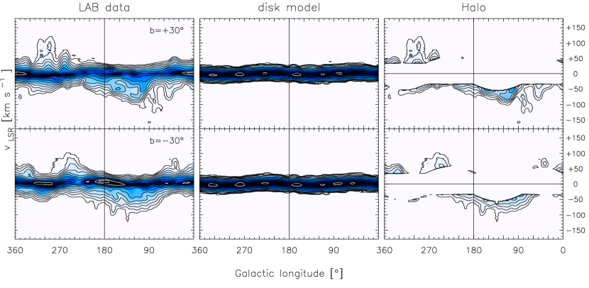
Figure 2: Longitude-velocity diagrams at latitudes $\pm 30^{\circ}$ above and below the mid-plane of the Galaxy. Left panels: LAB survey. Middle panel: disc model used throughout this paper. Right panel: LAB survey after the region of the disc has been removed, the remaining emission is used to compared our models with the data. Each datacube is smoothed to $8^{\circ}$ resolution. Contour levels in brightness temperature range from $0.04\,{\rm K}$ to $81.92\,{\rm K}$ scaling by a factor $2$.

2.3 Supernova-driven gas accretion

The pure galactic fountain model described above is modified to include interaction with the coronal gas according to FB08. We assume that the main mechanism at work is that described by Marinacci et al. (2010): the Kelvin-Helmholtz instability generates a turbulent wake behind each cloud in which material stripped from the cloud mixes with coronal gas, enhancing the metallicity and density of the latter and substantially decreasing its cooling time. As a consequence, part of the corona condenses into the wake and the mass of “cold” gas increases. The combined mass of cold gas in the cloud and the wake grows with distance along the cloud’s path through the halo very much as proposed by FB08. We demonstrate this quantitatively in Section 5.1.

Condensation in the wake modifies the kinematics of the cold gas in a way that depends on the kinematics of the corona. The latter is not known a priori, but must be strongly influenced by this interaction because the portion of the corona that interacts with fountain clouds does not contain much mass, and the interaction has been taking place throughout the disc’s lifetime. FB08 considered the effect of the drag between the clouds and the corona and concluded that, if there were no exchange of gas between the clouds and the corona, ram pressure between the cloud and the corona would force the corona to corotation with the cold gas in a time shorter than the fountain’s dynamical time. In reality much of the coronal gas that acquires momentum from a fountain cloud subsequently condenses in the cloud’s wake, so the momentum that is transferred to the coronal gas is in the end not lost by the whole body of cool gas. Marinacci et al. (2011) studied the transfer of momentum between fountain clouds and the corona in hydrodynamical simulations and found that there is a net transfer of momentum to the corona until the speed at which the clouds move through the corona falls to $50-100\,{\rm km\,s}^{-1}$, depending on the physical properties of the system. Below this threshold speed, net momentum transfer to the corona ceases as a result of coronal gas cooling in the cloud’s wake. In view of the short timescale on which ram-pressure can change the rotation rate of the corona, it is natural to assume that the corona has reached the velocity at which all the angular momentum imparted by ram pressure is subsequently recovered through condensation of coronal gas in the wake. Thus we assume that the rotation velocity of the corona is

$$v_{\phi}(R,z)=\sqrt{R\frac{\partial\Phi(R,z)}{\partial R}}-v_{\rm lag},$$ (5)

where $\Phi(R,z)$ is the potential of the Galaxy and $v_{\rm lag}=75\,{\rm km\,s}^{-1}$ is the (constant) velocity offset between clouds and corona at which condensation recaptures angular momentum transferred by ram pressure.

In this picture, the mass of cold gas (cloud$+$wake) associated with any cloud increases as

$$\dot{m}=\alpha m,$$ (6)

where $\alpha$ is the condensation rate, while the combined effect of condensation and drag decreases the velocity centroid of the cold gas at a rate (FB08)

$$\dot{v}=-\left(\alpha+\frac{1}{t_{\rm drag}\left(1+t/t_{\rm drag}\right)}\right)(v-v_{\phi})$$ (7)

where $t_{\rm drag}$ is the time at which the relative velocity between the cold gas and the corona halves due to the drag only. Since $t_{\rm drag}\!\propto\!|v-v_{\phi}|^{-1}\!\sim\!v_{\rm lag}^{-1}$, the drag efficiency decreases as the kinematics of the corona approaches that of the disc. We assumed a constant value for $t_{\rm drag}$ of $800\,{\rm Myr}$, according to the results of Marinacci et al. (2011) for $|v-v_{\phi}|=75\,{\rm km\,s}^{-1}$ (see Section 5.1), and we fitted the parameter $\alpha$. As we see below (Section 3.2), in order to reproduce the data we need $\alpha\!>\!1/t_{\rm drag}$, i.e. the condensation is the dominant process at work, while the drag plays only a secondary role. Note that fixing $t_{\rm drag}$ at $800\,{\rm Myr}$ implies that we are considering clouds with masses and sizes similar to those of Marinacci et al.’s simulations ($\sim 10^{4}\,{M}_{\odot}$, $100\,{\rm pc}$).

2.4 Comparison with the data

The comparison between the models and the data is performed by building model datacubes that resemble the LAB datacube (see FB06 and MF11). After each timestep of the integration, the positions and velocities of the particles are projected along the line of sight of an observer located in the mid-plane of the Galaxy, at a radius $R_{0}=8.5\,{\rm kpc}$, and moving at a circular speed $v_{\rm LSR}=220\,{\rm km\,s}^{-1}$. Using the same gas density for each cloud, we construct from these positions and velocities an artificial datacube. The artificial datacube is smoothed to $8^{\circ}$ resolution and then compared with the LAB datacube at the same resolution. The comparison is performed only in the portion of $(l,b,v_{\rm LOS})$ space to which the thin disc should not contribute. Following Wakker (1991), we use the deviation velocity $v_{\rm DEV}$ to identify this region. We model the footprint of the thin disc as described in MF11 and exclude data with $|v_{\rm DEV}|<35\,{\rm km\,s}^{-1}$. We also excluded the H I emission of the Magellanic Clouds and Stream, the Stream’s Leading Arm, the GCP complex, the Outer Arm and all external galaxies. In the following we refer to the surviving part of $(l,b,v_{\rm LOS})$ space as the halo region. The total model flux in the halo region is normalized to the corresponding LAB flux. This step fixes the mass of the H I halo.

Although the quantitative comparison between models and data is done only in the halo region, in all the plots of this paper a thin disc has been added for presentation purposes. This disc has a density profile taken from Binney & Merrifield (1998) and a scale-height taken from Kalberla et al. (2007). The velocity dispersion decreases linearly from $12\,{\rm km\,s}^{-1}$ in the Galactic centre to $6\,{\rm km\,s}^{-1}$ at $R_{0}$, and it remains constant at larger radii.

The leftmost column of Fig. 2 shows two longitude-velocity ($l,v$) plots at latitudes $\pm 30^{\circ}$ extracted from the LAB survey. The middle column of the same figure shows our model disc and the rightmost column shows the emission in the halo region of the LAB datacube. All the plots are centered at the anti-centre ($l\!=\!180^{\circ})$. Note that our cut is rather conservative and there should be no contamination from disc emission in the halo region.

In the application of the model to external galaxies, the fountain clouds have been modelled as point particles because individual clouds, with typical sizes $\sim 100\,{\rm pc}$, were unresolved in the data (FB06). In the Milky Way nearby clouds and their wakes will be resolved, so we have to check at each time step whether the combined emission of a cloud and its wake is resolved at the angular resolution of the data. If the emission is resolved, we spread the flux in a circular region around its centre. The flux density is assumed to decrease Gaussianly with distance from the centre, with FWHM equal to the apparent size of the cloud and its wake. Given that the data are used at $8^{\circ}$ resolution, a cloud and its wake are resolved only if their distance is smaller than $700\times\frac{D_{\rm cl}}{100\,{\rm pc}}\,{\rm pc}$, where $D_{\rm cl}$ is the system’s lengthscale. According to the simulations of Marinacci et al. (2010), turbulent wakes have sizes of $1-2\,{\rm kpc}$, so they will be resolved out to distances of about $10\,{\rm kpc}$. The pattern of emission from a cloud and its wake is quite elongated, having axis ratio $\sim 0.5$, but the long axis of the emission is randomly orientated, so our circular Gaussian smoothing should provide an adequate representation of the total emission from an ensemble of clouds. We tested the effect of resolution by increasing $D_{\rm cl}$ up to $2\,{\rm kpc}$ and found that the model datacube looked just like a smoothed version of that produced with smaller values of $D_{\rm cl}$. In the following we use models with small clouds, $D_{\rm cl}=200\,{\rm pc}$, for which the datacube can be computed significantly more quickly.

Once we have a model datacubes at the same resolutions and with the same total flux as the LAB datacube, we compare them quantitatively by calculating the residuals between them. This calculation is performed by adding up the differences between the models and the data, pixel by pixel, in the halo region. We used absolute differences, squared differences and also weighted residuals, i.e. $|$data$-$model$|/$(data$+$model). The residuals are calculated for a set of models with different input parameters such as the kick velocities $h_{\rm v}$ of the fountain clouds, and the model with the smallest residuals is our “best model”. In the following section we describe our best pure fountain model and our best fountain $+$ condensation model, showing that the latter provides a better description of the Galaxy’s H I data.

3 Results

3.1 A pure galactic fountain

Figure 3: Residuals between models and data as a function of $f_{\rm ion}$ for the pure galactic fountain with $h_{\rm v}=70\,{\rm km\,s}^{-1}$, evaluated using absolute differences (solid line), squared differences (short-dashed line) and weighted differences (long-dashed lines). All residuals have been divided by their respective minimum.

In a pure galactic fountain, the angular momentum of clouds is constant and orbits depend only on the characteristic kick velocity $h_{\rm v}$ of the clouds. However, the shape of the model datacube is also affected by the ionised fraction $f_{\rm ion}$, which has to be treated as a freely variable parameter.

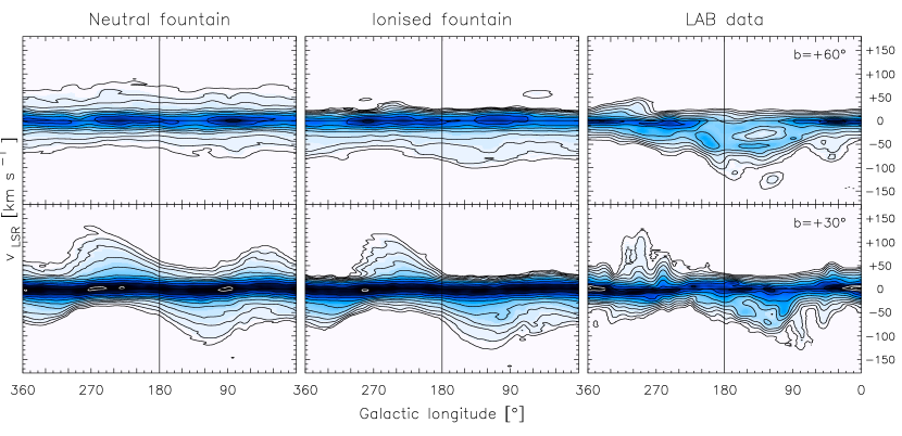
Figure 4: Longitude-velocity ($l,v$) diagrams at $b\!=\!60^{\circ}$ (top panels) and $b\!=\!30^{\circ}$ (bottom panels). First column: pure fountain model without phase-change ($f_{\rm ion}=0$); second column: best pure fountain model ($f_{\rm ion}=1$); third column: the LAB data. Each datacube is smoothed to $8^{\circ}$ resolution. Contour levels in brightness temperature range from $0.04\,{\rm K}$ to $81.92\,{\rm K}$ scaling by a factor $2$.

We have calculated the residuals for $h_{\rm v}$ in the range $(30,120)\,{\rm km\,s}^{-1}$ and $f_{\rm ion}$ between $0$ and $1$. The weighted and non-weighted residuals give different results but the confidence contours overlap for $h_{\rm v}\simeq 70\,{\rm km\,s}^{-1}$ and $f_{\rm ion}=1$. In Fig. 3 we show the normalized residuals as a function of $f_{\rm ion}$ for $h_{\rm v}\!=\!70\,{\rm km\,s}^{-1}$. Clearly the differences between models and data decrease as $f_{\rm ion}$ approaches $1$, regardless of the method of comparison. The mass of the H I halo derived for this model is $M_{\rm halo}=5.2\times 10^{8}M_{\odot}$. Here and below the halo masses are estimated by excluding fountain clouds at $|z|\!<\!0.4\,{\rm kpc}$, which is roughly the blowout height of a superbubble (see Spitoni et al., 2008). Taking into account also clouds at heights $0.2\!<\!|z|\!<\!0.4\,{\rm kpc}$, the H I halo mass would become $M_{\rm halo}=7.2\times 10^{8}M_{\odot}$.

Fig. 4 shows two representative $l,v$ diagrams (centred on the anticentre) at latitudes $b\!=\!60^{\circ}$ and $b\!=\!30^{\circ}$ for: the best pure galactic fountain model (middle column); the same model without phase-change (left column); the data (right column). The difference between the two models is striking, especially at higher latitudes. The $l,v$ plots for the neutral ($f_{\rm ion}=0$) fountain are rather symmetric with respect to the zero velocity line. In the ionised fountain by contrast, the gas appears systematically located at negative velocities. This effect is a consequence of clouds of the ionised fountain being visible only as they fall back to the disc. The data clearly display this preference for more negative than positive velocities.

The leftmost column in Fig. 6 shows additional $l,v$ diagrams for the best pure fountain model. It reproduces the most prominent features, so it gives a good description of the data. It is interesting to compare Fig. 6 with Fig. 6 of MF11, which shows the prediction of an optimised kinematic model. In several locations the dynamical model fits the data better than the best kinematic model of MF11. For example, at latitudes $b=\pm 15^{\circ}$ the superiority of the present model is very clear in the central regions of the Galaxy, $0^{\circ}<l<60^{\circ}$ and $300^{\circ}<l<360^{\circ}$. At latitudes $b=\pm 30^{\circ}$, the superiority is clear at $l\sim 270^{\circ}$ ($-90^{\circ}$ in MF11).

The kinematic model was built under the assumption that the scaleheight and kinematic parameters of the halo (rotation velocity gradient, vertical and radial velocities) are independent of radius. Although the assumption is restrictive, the model has been fitted to the data by freely varying these quantities, regardless of their dynamical plausibility. The fact that a dynamical model with only two free parameters fits the data better is remarkable, and strongly supports the idea that the H I halo of the Milky Way is produced by supernova feedback from the Galactic disc.

Table 1: Best galactic fountain models for the Milky Way.

Fountain model	$h_{\rm v}$	$M_{\rm HI}^{~{}~{}~{}a}$	$M_{\rm HI+HII}^{~{}~{}~{}~{}~{}~{}~{}~{}~{}a}$	$f_{\rm ion}$	$\alpha$	$M_{\rm accr}$	Residualsc
	($\,{\rm km\,s}^{-1}$)	($\,{M}_{\odot}$)	($\,{M}_{\odot}$)		(Gyr-1)	($\,{M_{\odot}\,\rm yr}^{-1}$)
Neutral (pure)	$70^{b}$	$4.6\times 10^{8}$	$4.6\times 10^{8}$	$0.0^{b}$	$0.0^{b}$	0.0	1.60
Ionised (pure)	70	$5.2\times 10^{8}$	$10.4\times 10^{8}$	$1.0$	$0.0^{b}$	0.0	1.48
With corona condensation	70	$2.7\times 10^{8}$	$3.0\times 10^{8}$	0.3	6.3	1.6	1.26

^a estimated above $400\,{\rm pc}$ from the plane; ^b fixed; ^c calculated as absolute differences, the closer to 1 the better the fit.

3.2 Including the condensation of the corona

Figure 5: Contour plots of residuals between models with corona condensation and data evaluated in the parameter space ($\log(\alpha)$,$f_{\rm ion}$) for $h_{\rm v}=70\,{\rm km\,s}^{-1}$. Different panels compare models and data in different ways, as labelled on bottom. In each panel all values have been divided by the respective minimum. The fourth panel is the sum of the previous three, divided by the resulting minimum. Contour levels at $1.005,1.01,1.02,1.05$.

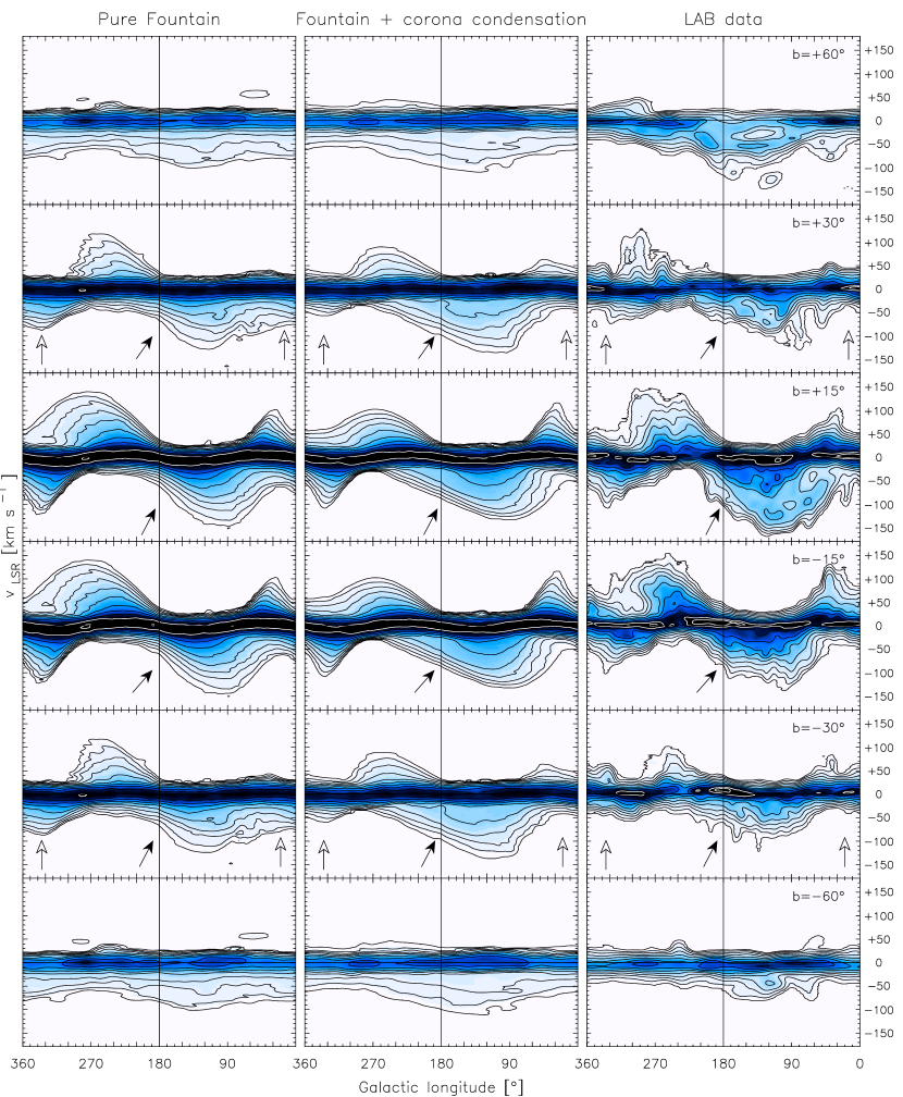
Figure 6: $l,v$ slices at 6 different latitudes indicated at the top right corner of the rightmost plots. First column: best pure Galactic fountain; second column: best fountain with condensation of the corona; third column: the LAB data. Each datacube is smoothed to $8^{\circ}$ resolution. Contour levels in brightness temperature range from $0.04\,{\rm K}$ to $81.92\,{\rm K}$ scaling by a factor $2$. The arrows show regions where radial motions are present and the model with coronal condensation reproduces the data better than the pure fountain model, see text.

The best pure fountain model described above is extreme in that it requires the full ionisation of ejected clouds and a large mass of the gaseous halo (see Table 1). Moreover there are several locations in the datacube where the model systematically fails to reproduce the data in detail. The arrows in Fig. 6 indicate such regions. In these regions radial motions are important. For instance filled arrows show the region around the anticentre, $150^{\circ}<l<250^{\circ}$, where the data, almost at every latitude, have a broader distribution in velocity than the pure fountain model. Gas in this region is flowing towards the centre of the Galaxy from beyond the Solar circle. In a pure galactic fountain, orbits seldom move in this way (FB06) and independently of the ionised fraction they do not produce much emission in the marked region.

We now show that including the interaction between clouds and the corona as described in Section 2.3 substantially improves this situation. The interaction is parametrised by the specific condensation rate $\alpha$. The larger $\alpha$ is, the faster gas condenses from the corona, the greater the rotational lag of the H I, and the more prominent is inward radial motion of H I (see FB08).

Now the residuals between the data and the models are minimised by varying three parameters ($h_{\rm v},f_{\rm ion},\alpha$). We assume that condensation and drag are suppressed close to the Galactic plane ($|z|<0.4\,{\rm kpc}$). A full analysis of this three-dimensional parameter space would be too expensive computationally, so we explore only the space ($\alpha$,$f_{\rm ion}$) and fix the kick velocities at three values: $h_{\rm v}=60$, $70$ and $80\,{\rm km\,s}^{-1}$. For each value of $h_{\rm v}$ we build a map of the residuals between models and data by varying the other parameters in the ranges $0<f_{\rm ion}<1$ and $-3<\log(\alpha/\,{\rm Gyr}^{-1})<-1.67$ with a step of $0.033$ in both directions. This map is then smoothed to the resolution of $0.1\times 0.1$ in order to minimise the stochastic effects due to the probability distribution function (eq. 1) used to build our models. As in the case of a pure fountain, different residuals give different results. Regardless of $\alpha$ and $f_{\rm ion}$, absolute and squared differences have lower values for $h_{\rm v}=80\,{\rm km\,s}^{-1}$, while relative residuals favour $h_{\rm v}=60\,{\rm km\,s}^{-1}$. Hence we set our kick velocity in the middle and focus on models with $h_{\rm v}=70\,{\rm km\,s}^{-1}$.

The first three panels in figure 5 show the residual maps obtained with $h_{\rm v}=70\,{\rm km\,s}^{-1}$ for different types of residuals. In each panel all values are divided by the respective minimum, thus they are dimensionless and $\geq 1$. Combining these three panels we obtain the fourth (rightmost) panel, which is the sum of the previous three divided by the resulting minimum, which occurs at $f_{\rm ion}=0.3$ and $\log(\alpha)=-2.2$ (so $\alpha=6.3\,{\rm Gyr}^{-1}$). For this best model the mass of the H I halo is $2.7\times 10^{8}M_{\odot}$. Table 1 lists the parameters.

The middle column of Fig. 6 shows that the model with coronal condensation reproduces the emission near the anticentre better than the pure fountain model. The open arrows (latitudes $b=\pm 30^{\circ}$) indicate other regions where the inclusion of coronal condensation improves the fit to the data. These are regions in which H I is flowing out from the inner disc, and the pure fountain provides too much emission.

For our best-fitting value of $\alpha$, the condensation rate of coronal gas into the clouds’ wakes is $\dot{M}=1.6\,{M_{\odot}\,\rm yr}^{-1}$. Correcting this value for the He content increases the condensation rate to $2.3\,{M_{\odot}\,\rm yr}^{-1}$. This value is remarkably close to the Galaxy’s SFR, which we assume to be $\sim 3\,{M_{\odot}\,\rm yr}^{-1}$ (Diehl et al., 2006), of which $\sim 1\,{M_{\odot}\,\rm yr}^{-1}$ should be accounted for by gas ejected from stars in the disc. We consider it highly significant that $\dot{M}$ deduced from an H I survey should agree so well with that required to sustain the SFR, which is obtained without reference to H I.

The exact value of the condensation rate $\dot{M}$ depends on several factors. An important parameter is the value of $v_{\rm lag}$ (eq. 5), which regulates the rotation of the corona and therefore the efficiency of both the drag ($t_{\rm drag}\propto v_{\rm lag}^{-1}$) and the condensation (Marinacci et al., 2011). However, experiments show that the dependence of $\dot{M}$ on the adopted value of $v_{\rm lag}$ is not strong: ($v_{\rm lag}=50\,{\rm km\,s}^{-1},\,t_{\rm drag}=1200\,{\rm Myr})$ yields $\dot{M}=2.8\,{M_{\odot}\,\rm yr}^{-1}$ ($3.9\,{M_{\odot}\,\rm yr}^{-1}$ when corrected for He), while ($v_{\rm lag}=100\,{\rm km\,s}^{-1},\,t_{\rm drag}=600\,{\rm Myr}$) yields $\dot{M}=1.0\,{M_{\odot}\,\rm yr}^{-1}$ ($1.4\,{M_{\odot}\,\rm yr}^{-1}$ when corrected for He). It is interesting to note that $\dot{M}$ depends very little on the criterion used to minimise the residuals. Although the three criteria yield rather different values for the best-fitting $\alpha$ (see Fig. 5), $\dot{M}$ only varies between 1.5 and 1.7$\,{M_{\odot}\,\rm yr}^{-1}$ given that the halo masses also vary between the three models.

Our parametrisation assumes that $\alpha$ is spatially constant. Fortunately, the density of the corona should not vary too much in the regions where the interaction with the fountain is efficient (Marinacci et al., 2011), so spatial variation of $\alpha$ is not expected to give significantly different results.

On the whole, the dynamical modelling of the Galactic H I halo performed in this work is a success. The results are consistent with the conclusions MF11 drew from their kinematic models. They found negative values for both the average vertical and the radial velocities of the halo material, and deduced that ejected clouds must be partially ionised (but in a fraction larger than our current determination). Our dynamical analysis identifies these properties as arising from the sharing of angular momentum with gas accreted from the lagging corona. Finally, our Galactic fountain is dynamically sustainable. It requires a rate of kinetic-energy injection equal to $6.2\times 10^{39}{\rm erg}\,{\rm s}^{-1}$, which with a supernova rate SNR$\,=0.03\,{M_{\odot}\,\rm yr}^{-1}$ and an energy per supernova of $1\times 10^{51}{\rm erg}$ corresponds to an efficiency of about 0.7%.

4 Properties of the Galactic H I layer

Now that we have a model that reproduces all the main features of the LAB datacube, we can investigate in detail the physical properties of the Galaxy’s extraplanar H I layer.

4.1 Rotation versus height

Figure 7: Rotational velocities for the H I layer of the Milky Way at different heights from the plane (thin lines), compared to the disc rotation curve (thick line). The velocities are derived from our best mixing fountain model by taking the weighted average of $v_{\rm\phi}$ at that $(R,z)$ location.

Fig. 7 shows the rotation curve of the Galaxy’s extra-planar gas at different distances from the plane as a function of $R$. These values were derived from our best model by simply taking the weighted mean of the azimuthal components of the velocities of the particles at different heights. As expected, the halo gas is lagging the rotation of the disc (black curve). Roughly 50% of this lag is due to gravity (FB06) whilst the other half is produced by a combination of the interaction with the corona and the phase-change. At $R_{0}$ the gradient is about $-14.3\pm 1.1\,{\rm km\,s}^{-1}\,{\rm kpc}^{-1}$ in excellent agreement with the average value derived in the inner regions of the Milky Way by MF11 ($-15\pm 4\,{\rm km\,s}^{-1}\,{\rm kpc}^{-1}$), which also coincides with the value derived for NGC 891 by Oosterloo et al. (2007).

4.2 Thickness of the H I layer

A second fundamental property of the Galaxy’s H I halo is its thickness. To obtain it we fitted the vertical density profiles in our models at different radii with exponential functions. Fig. 8 shows the (exponential) scale-height of the H I halo of our best model as a function of $R$. The thickness increases with $R$ because the gravitational restoring force to the plane diminishes outwards (FB06). The halo density decreases abruptly for $R\!>\!14\,{\rm kpc}$, so its thickness cannot be reliably determined at larger radii. The shape of the scaleheight as a function of R is partially due to the assumption of our model that the kick velocity $h_{\rm v}$ does not change with radius (for a discussion see FB06). In the inner Galaxy there has long been evidence for a population of H I clouds extending up to $\sim 1\,{\rm kpc}$ above the midplane (Lockman, 1984, 2002; Ford et al., 2010). Marasco & Fraternali (2011) assumed a constant thickness for the halo and derived a value of $1.6\,{\rm kpc}$ using a $\rm{sech}^{2}$ formula, which corresponds to $\sim 800\,{\rm pc}$ for an exponential function. This value agrees well with the average of the scaleheights plotted in Fig. 8.

Figure 8: Scale-height as a function of $R$ for our best halo model including condensation of the coronal gas.

Kalberla et al. (2007) studied the vertical structure of the Galaxy’s H I layer on the assumption that the layer is in hydrostatic equilibrium. Using this assumption, they inferred that while at $R_{0}$ the H I layer extends only a few hundred parsecs from the plane, at $R\simeq 35\,{\rm kpc}$ the vertical structure of the H I layer can be fitted by a Gaussian distribution with scale height $2.5\,{\rm kpc}$. Thus they deduced a very extended H I layer with strong flaring. They also inferred the existence of a massive ring of dark matter between $R=13$ and $18.5\,{\rm kpc}$. The assumption of hydrostatic equilibrium leads, however, to models that fail to match the data correctly (see Barnabè et al., 2006; Marinacci et al., 2010). If Kalberla et al. (2007) had used the prediction of a fountain model for the distribution of H I near $R_{0}$ rather than a model based on hydrostatic equilibrium, they would have come to different conclusions regarding the radii responsible for each quantity of emission in the H I datacube. Consequently, the distribution of the matter and the structure of the H I flare in the Milky Way should be re-derived. While this topic merits further work, our comparisons of the fountain model with the data yield no compelling evidence for substantial flaring of the H I layer much beyond $R\sim 15\,{\rm kpc}$.

4.3 Accretion and circulation of gas

Figure 9: Hydrogen flow as function of $R$ predicted by our best model with condensation of the corona. Inflows (outflows) are represented by positive (negative) values. Top panel: net flow ($\hbox{inflow}-\hbox{outflow}$) produced by the Galactic fountain. Bottom panel: accretion of pristine gas from the corona onto the disc. The global accretion rate is $1.6\,{M_{\odot}\,\rm yr}^{-1}$.

Infall of metal-poor gas to the star-forming disc is an essential ingredient of current models of the Galaxy’s chemical evolution (e.g. Chiappini et al., 2001; Schönrich & Binney, 2009). The predictions of such models depend to a significant extent on the radial profile of the infall, but hitherto there has been no credible way of determining this profile. The prediction of our model for this profile is shown in Fig. 9 (bottom panel). The curve shows the pristine gas that, condensing from the corona onto the fountain cloud wakes, follows the cloud orbits back to the disc. The shape of the accretion profile is due to the variation of the mass outflow and the orbital time with radius. At $R\la 3\,{\rm kpc}$ the specific accretion rate essentially vanishes because the orbits of the fountain clouds are confined within few hundred of parsecs from the disc (see Fig. 8). It then rises to a peak at $R\simeq 9\,{\rm kpc}$ as in this region both the orbital time and the star formation are sufficiently high. At $R>9\,{\rm kpc}$ the accretion rate falls again due to the low level of star formation at these radii, and drops to about zero beyond $R=13\,{\rm kpc}$. The integral of this curve over the disc surface gives a global accretion rate of $\dot{M}=1.6\,{M_{\odot}\,\rm yr}^{-1}$. Note that the peak in the accretion rate lies well beyond the peak in the Milky Way’s SFR, which occurs around $R\!=\!4\,{\rm kpc}$. This implies the need for a redistribution of gas in the disc, the study of which is beyond the scope of the present paper (but see for instance Schönrich & Binney, 2009; Spitoni & Matteucci, 2011).

The top panel of Fig. 9 shows the net flow (H I+H II) as function of $R$, obtained as the difference between the rate at which gas arrives at a given radius and the rate at which supernovae eject gas from that radius. The net flow profile differs from the accretion profile because fountain clouds do not fall back onto the disc at the same radius they are ejected from. As $R$ increases, the orbits of fountain clouds start to get an inward component because of the interaction with the corona, thus clouds land at smaller and smaller radii. In particular, most of the clouds ejected at $11\!<\!R\!<\!15\,{\rm kpc}$ fall back onto the disc at $6\!<\!R\!<\!11\,{\rm kpc}$. As a consequence, a ‘draining region’ forms at $11\!<\!R\!<\!15\,{\rm kpc}$, while inside this annulus the amount of gas falling onto the disc significantly exceeds the outflowing counterpart: about $70\%$ of this inflow comes from the condensation of the corona, the remaining part is due to the described gas circulation. On the whole, the fountain circulation contributes to $76\%$ of the halo mass, while the accreted gas is $24\%$. This latter is similar to that derived by FB08 for NGC 891 and NGC 2403 ($\sim 10-20\%$).

4.4 HVCs and IVCs

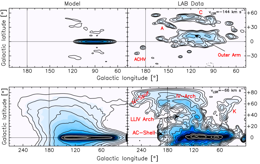
Figure 10: Channel maps at $v_{\rm LSR}\!=\!-144\,{\rm km\,s}^{-1}$ (top) and $v_{\rm LSR}\!=\!-66\,{\rm km\,s}^{-1}$ (bottom) for our best model with coronal condensation (left panels) and the LAB data (right panels). Both model and data are smoothed to $4^{\circ}$ resolution. Contour levels in brightness temperature range from $0.04\,{\rm K}$ to $81.92\,{\rm K}$ scaling by a factor $2$. Some of the high and intermediate-velocity complexes are labelled (see text).

At large line-of-sight velocities the H I emission in the halo region of our Galaxy is dominated by the HVCs, the emission from which lies in rather isolated outlying regions of $(l,b,v)$ space delimited by $|v_{\rm DEV}|>90\,{\rm km\,s}^{-1}$ (van Woerden et al., 2004). The upper panels in Fig. 10 compare the emission predicted by our best model (left panel) near $v_{\rm LSR}\!=\!-144\,{\rm km\,s}^{-1}$ with what is actually observed. In the observational data, three main islands of emission are apparent. At $b>30^{\circ}$ we see Complexes A and C, which have no real counterparts in the model. Similarly emission at $l\ga 180^{\circ}$ associated with the Anticentre High-Velocity Cloud (ACHV) has no counterpart in the model. It is well known that the metallicity of most HVCs, in particular Complexes A and C is much lower than that of gas in the disc, which strongly suggests that they come from outside the Galaxy (see Wakker, 2001). Moreover, assuming a distance of $10\,{\rm kpc}$ for both Complexes A and C (van Woerden et al., 2004; Thom et al., 2008) gives for these objects heights from the midplane of $6-8\,{\rm kpc}$. To produce emission so far from the plane, we would need a kick velocity $h_{\rm v}\gtrsim 150\,{\rm km\,s}^{-1}$. A model with $h_{\rm v}$ so large completely fails to reproduce the data globally. In summary, HVCs such as Complexes A and C are almost certainly extragalactic in origin and our model is quite correct not to reproduce them. The rate at which the Galaxy accretes gas from infalling HVCs is $\sim 0.2\,{M_{\odot}\,\rm yr}^{-1}$ (Sancisi et al., 2008), an order of magnitude lower than our estimate of the rate of accretion via the fountain $+$ corona condensation mechanism.

The main body of emission in the upper right panel of Fig. 10 forms a large island that straddles the plane. Its summit lies at $(l,b)=(120^{\circ},15^{\circ})$ and is labelled “Outer Arm”. This feature is thought to arise from the warp of the H I disc. Our model (left panel) does not include a warp in the disc, so apart from two horns of very faint emission either side of the plane, its emission is confined in a thin region around the plane.

The lower panels of Fig. 10 show predicted (left) and observed (right) emission at much lower heliocentric velocities ($v_{\rm LSR}\!\simeq\!-66\,{\rm km\,s}^{-1}$) than the upper panel. At such Intermediate Velocities (IVCs are classically defined to be at $35\,{\rm km\,s}^{-1}\!<\!|v_{\rm DEV}|\!<\!90\,{\rm km\,s}^{-1}$) the model is seen to reproduce the global structure of the data very well. Moreover, some of the IVCs that contribute to this emission have been shown to have a distance from the Sun of $\la 3\,{\rm kpc}$ and disc-like metallicities (van Woerden et al., 2004), consistent with their being fountain clouds. In the lower-right panel of Fig. 10 several IVCs are visible (IV-Arch, IV-Spur, LLIV-Arch, AC-Shell, Complex K), mainly at positive latitudes. The emission of our model is smoother than the data, but apart from that it is consistent with the existence of all the IVCs.

The classical IVCs shown in the lower right panel of Fig. 10 must be just the most conspicuous members of a large population of IVCs that collectively comprise the H I halo (see also MF11). By assuming azimuthal symmetry, our model suppresses much of the noise inherent in observing a population of discrete clouds. In principle one could hope with a more sophisticated model to reproduce the statistical properties of this noise, but there is no particular merit in reproducing individual IVCs, which will just be the chance, and ephemeral, products of individual bursts of star formation.

If IVCs contain a mixture of metal-rich gas ejected from the disc and gas condensed from the rather metal-poor corona, the metallicities of these clouds should be intermediate between those of the disc and corona. Since the fraction of accreted material is $\sim 24\%$ of the whole halo mass, the IVCs should be somewhat more metal-poor than the disc.

5 Discussion

5.1 Analytic approximation vs hydrodynamical simulations

In Section 2.3 we pointed out that our assumption of exponential growth of the mass of the cold gas is qualitatively similar to that observed by Marinacci et al. (2010) in their hydrodynamical simulations of cold clouds travelling through a hot medium. Here we show that this agreement is quantitatively sound.

The points in the upper panel of Fig. 11 show the mass of coronal gas that has $T<3\times 10^{4}\,{\rm K}$ in the simulations of Marinacci et al. (2011); the units are fractions of the initial mass of the cloud. The curve shows the mass accreted by a particle that after $38\,{\rm Myr}$ starts to accrete according to equation (6) with the growth rate set to the value, $\alpha=6.3\,{\rm Gyr}^{-1}$, determined by our fits to the LAB datacube (Table 1). The fit in Fig. 11 between the curve and the data points from Marinacci et al. (2010) is excellent. We interpret the delay by $38\,{\rm Myr}$ before accretion starts as the time required for cold gas from the cloud to mix with the coronal gas plus the time required for the coronal gas to cool to $T<3\times 10^{4}\,{\rm K}$.

Figure 11: Top panel: The square points show the mass of coronal gas that condensed into the cloud wake as a function of time extracted from the simulations of Marinacci et al. (2011). Bottom panel: The square points show the velocity centroid of cold gas in the simulations of Marinacci et al. (2011), the dashed curve shows the prediction in case of drag ($t_{\rm drag}=800\,{\rm Myr}$) without condensation. In each panel the solid curves show the predictions of the inelastic collision+drag recipe used in this work (equation 7).

The points in the lower panel of Fig. 11 show the velocity of the cold-gas centroid in the simulations of Marinacci et al. (2011). The dashed line shows the evolution of the velocity if the cloud were a rigid body that experienced hydrodynamical drag as described in FB06 with $t_{\rm drag}\!=\!800\,{\rm Myr}$. This line fits the data from Marinacci et al. (2011) well until $t\simeq 20\,{\rm Myr}$. At later times the full thick curve shows the prediction for the combined effects of drag and condensation, obtained from equation (7) using again $\alpha=6.3\,{\rm Gyr}^{-1}$. The required condensation rate is very similar than that predicted by the simulations.

It is remarkable that detailed hydrodynamical simulations yield a value of the accretion rate $\alpha$ that agrees so well with the value we obtained by fitting the H I datacube because the only connection between these two determinations is the underlying physics of turbulence. It is true that to obtain the agreement we did have to choose a value for the delay between the start of a hydrodynamical simulation and the onset of effective cooling. Some delay is inevitable because the hydrodynamical simulations start with unrealistically spherical clouds and no wake. More realistic initial conditions for the dynamics of gas expelled from the disc by a superbubble would yield a time shorter than $30-40\,{\rm Myr}$ for steady accretion to become established.

The simulations of Marinacci et al. (2011) last only 60 Myr; new simulations that also include gravity are now being carried out (Marinacci et al., in preparation). These show that the cold gas (cloud $+$ wake) falls back to the disc in rather coherent structures with sizes of $1-1.5\,{\rm kpc}$ and after times also larger than 60 Myr and comparable to the ballistic travel times.

While our choice of temperature threshold at $T=3\times 10^{4}\,{\rm K}$ for gas to become visible as H I is somewhat arbitrary, experimenting with different temperature thresholds we found that the trends of mass and velocity are perfectly comparable with the one shown here (F.  Marinacci, private communication).

In conclusion, the analytical treatment of an inelastic collision between fountain particles and ambient gas proposed by FB08 and adopted here is quantitatively supported by the numerical simulations of Marinacci et al. (2011). The system of cloud $+$ turbulent-wake accretes mass and looses specific momentum in the way predicted by the analytical formula. Remarkably the rate at which this process occurs in the simulations is the same as the rate we estimated by fitting models to the LAB survey data.

5.2 Comparison to other galaxies

FB06 and FB08 applied the model discussed here to two external galaxies, the Milky Way-like NGC 891, and the M33-like NGC 2403. For the former the kick velocities necessary to reproduce the data were in the range $70-90\,{\rm km\,s}^{-1}$ depending on the shape of the potential and the extent and type of gas accretion considered. For NGC 2403 the data could be reproduced with values of the initial kick velocity from $75\,{\rm km\,s}^{-1}$ down to about $50\,{\rm km\,s}^{-1}$. Thus the value of $70\,{\rm km\,s}^{-1}$ that minimises the residuals in the Milky Way is fully consistent with those needed to produced the H I halos of other galaxies. As discussed in FB06, these velocities are also consistent with hydrodynamical simulations of superbubble expansion (e.g. Mac Low et al., 1989).

The accretion parameters $\alpha$ estimated by FB08 for NGC 891 and NGC 2403 are a factor $3-7$ lower than that found here for the Milky Way. This would imply shorter timescales for the condensation of the ambient gas in the Milky Way. However, the value of $\alpha$ is linked to the rotational velocity assumed for the corona where it interacts with the fountain. FB08 assumed that the fountain gas interacted with a static ambient medium, which maximised the effect of the process. Had we considered such a configuration for our corona we would have found a condensation parameter $\alpha=2.5\,{\rm Gyr}^{-1}$. In this case $t_{\rm drag}\sim 300$, which implies that the drag dominates over the condensation. However, as explained in Section 2.3, a static (non-rotating) corona is not a realistic possibility.

6 Conclusions

Just as in the 1980s photometry of external galaxies proved the key to making sense of star counts within our Galaxy (Bahcall & Soneira, 1980), so it is natural to turn to studies of the H I distributions of external galaxies for help in interpreting the Galaxy’s H I datacube. In this paper we have investigated the extent to which the latter can be understood using a model of the extraplanar H I that emerged from observations of external galaxies such as NGC 891 and NGC 2403. In this model clouds of relatively cool gas are ejected from the plane by supernova-driven superbubbles and subsequently orbit over the disc on near ballistic trajectories whilst weakly interacting with the virial-temperature coronal gas through which they move. The interaction with the coronal gas is through a combination of ram-pressure drag and accretion of gas that cools in the cloud’s wake. As a result of this accretion, more gas returns to the plane than left it.

In light of recent developments, we modified the model slightly before applying it to the Galaxy. The principal modifications were (a) to allow for rotation of the corona, and (b) to change the rule for determining the SFR from one based on total gas density to one based on the density of molecular gas alone. Neither modification arises from a desire to fit data for the Galaxy better; (a) reflects an improved understanding of the hydrodynamics of cloud-corona interaction, and (b) arises from better data for external galaxies. A task for the future is to reanalyse the data for external galaxies using our present model.

Our model has three adjustable parameters, the characteristic velocity of cloud ejection $h_{\rm v}$, the specific accretion rate of clouds $\alpha$, and a dimensionless parameter $f_{\rm ion}$, which determines where along its trajectory the cloud’s gas, which is initially photoionised, becomes visible as H I. To fit the data we require $h_{\rm v}\simeq 70\,{\rm km\,s}^{-1}$, regardless of the assumptions we make about the values of $\alpha$ and $f_{\rm ion}$.

At high Galactic latitudes, the observations show a clear bias towards negative velocities, and from this fact it follows that $f_{\rm ion}$ has to be larger than zero. If we set $\alpha=0$, thus excluding accretion from the corona, we obtain a reasonable fit to the data with $f_{\rm ion}=1$, so clouds become neutral only when they start to move back towards the plane.

Permitting $\alpha$ to be non-zero yields fits to the data that are improved in small but significant ways. In particular, with $\alpha>0$, more emission is predicted at negative velocities at low latitudes and $l=180^{\circ}$. Also less emission is predicted at negative velocities and $|l|\simeq\pm 10^{\circ}$ and $|b|\simeq 30^{\circ}$. Both these changes arise from an increase in the extent of global inflow of the H I, and they improve the fit to the data. Moreover, with $\alpha\neq 0$ the optimum value of $f_{\rm ion}$ is reduced from unity to $0.3$, so clouds become neutral about $30$ percent of the way to their highest point above the plane. Our best-fitting model has $\alpha=6.3\,{\rm Gyr}^{-1}$, which implies that $1.6\,{M_{\odot}\,\rm yr}^{-1}$ of hydrogen is accreted from the corona. Including the He content, this value rises to $2.3\,{M_{\odot}\,\rm yr}^{-1}$. This accretion rate is in excellent agreement with estimates of the accretion rate required to sustain the Galaxy’s current rate of star formation without depleting its rather meagre stock of interstellar gas.

Unfortunately, two problems prevent us from tightly constraining the value of $\alpha$. The first is that it is inferred from some quite subtle features in the H I datacube. The second is that the optimum value of $\alpha$ depends on the value adopted for $v_{\rm lag}$, the equilibrium difference in the rotation velocities of the H I halo and the corona. When $v_{\rm lag}$ is raised to $100\,{\rm km\,s}^{-1}$, the optimum value of $\alpha$ decreases to $4.0\,{\rm Gyr}^{-1}$, which corresponds to an accretion rate of $1.0\,{M_{\odot}\,\rm yr}^{-1}$ ($1.4\,{M_{\odot}\,\rm yr}^{-1}$ including the He content).

Fig. 10 illustrates how successfully the model simulates H I emission at Intermediate Velocities – the simulation is probably as perfect as it can be without reproducing individual superbubbles. By contrast, the model does not reproduce emission at High Velocities, presumably because HVCs are extragalactic in origin.

We find remarkable agreement between the optimum values of the model’s parameters and the values found in earlier work. In particular, our value of $h_{\rm v}$ lies within the ranges of values found for NGC 891 and NGC 2403, and although our value for $\alpha$ is higher than that found for NGC 891 this difference can be traced to different assumptions regarding the rotation of the corona here and in the work of FB08 on NGC 891. Our value of $\alpha$ does beautifully reproduce the results of a simulation by Marinacci et al. (2011) of the hydrodynamics of cloud-corona interaction. Our value $dv_{\phi}/dz\simeq-14.3\,{\rm km\,s}^{-1}\,{\rm kpc}^{-1}$ for the vertical gradient of the halo’s mean-streaming velocity agrees perfectly with the value ($\sim-15\,{\rm km\,s}^{-1}\,{\rm kpc}^{-1}$) determined for NGC 891. These quantitative agreements between studies that use either radically different methodologies or data inspires confidence that our underlying physical picture is correct.

If we accept the fundamental soundness of the model, we can from it infer the three-dimensional structure of the H I halo, which is otherwise unknown. We find that the halo contains $\sim 3.0\times 10^{8}\,{M}_{\odot}$ of gas, of which $2.7\times 10^{8}\,{M}_{\odot}$ is neutral, in agreement with the value of $3.2^{+1.0}_{-0.9}\times 10^{8}\,{M}_{\odot}$ estimated by MF11. Its vertical scaleheight increases roughly linearly with radius from $\sim 250\,{\rm pc}$ at $R=3\,{\rm kpc}$ to $2\,{\rm kpc}$ at $R=14\,{\rm kpc}$. At larger radii the scaleheight falls along with the local SFR. This H I halo is neither in hydrostatic equilibrium nor strictly in circular rotation: an analysis of the data that is nevertheless based on the assumption of hydrostatic equilibrium and circular motion will yield a misleading structure for the H I disc, especially the flare. This structure will in turn lead to false conclusions about the distribution of matter required to gravitationally confine the H I disc (see Sect. 4.2). The rate per unit area at which the halo deposits coronal gas on the disc increases roughly linearly from near zero at $R=3\,{\rm kpc}$ to a peak at $R=9\,{\rm kpc}$ and then falls roughly linearly to near zero at $R=13\,{\rm kpc}$. Models of the chemical evolution of the disc need the accretion profile as an input, and it will be interesting to discover how the predictions of such models change when the present accretion profile is adopted.

References

- Anderson & Bregman (2010) Anderson M. E., Bregman J. N., 2010, ApJ, 714, 320
- Anderson & Bregman (2011) Anderson M. E., Bregman J. N., 2011, ApJ, 737, 22
- Aumer & Binney (2009) Aumer M., Binney J. J., 2009, MNRAS, 397, 1286
- Bahcall & Soneira (1980) Bahcall J. N., Soneira R. M., 1980, ApJL, 238, L17
- Balbus & Soker (1989) Balbus S. A., Soker N., 1989, ApJ, 341, 611
- Barbieri et al. (2005) Barbieri C. V., Fraternali F., Oosterloo T., Bertin G., Boomsma R., Sancisi R., 2005, A&A, 439, 947
- Barnabè et al. (2006) Barnabè M., Ciotti L., Fraternali F., Sancisi R., 2006, A&A, 446, 61
- Bauermeister et al. (2010) Bauermeister A., Blitz L., Ma C., 2010, ApJ, 717, 323
- Binney & Merrifield (1998) Binney J., Merrifield M., 1998, Galactic astronomy
- Binney et al. (2009) Binney J., Nipoti C., Fraternali F., 2009, MNRAS, 397, 1804
- Binney & Tremaine (2008) Binney J., Tremaine S., 2008, Galactic Dynamics: Second Edition. Princeton University Press
- Blitz et al. (1999) Blitz L., Spergel D. N., Teuben P. J., Hartmann D., Burton W. B., 1999, ApJ, 514, 818
- Boomsma et al. (2008) Boomsma R., Oosterloo T. A., Fraternali F., van der Hulst J. M., Sancisi R., 2008, A&A, 490, 555
- Bregman (2007) Bregman J. N., 2007, ARA&A, 45, 221
- Chiappini et al. (1997) Chiappini C., Matteucci F., Gratton R., 1997, ApJ, 477, 765
- Chiappini et al. (2001) Chiappini C., Matteucci F., Romano D., 2001, ApJ, 554, 1044
- Cignoni et al. (2008) Cignoni M., Tosi M., Bragaglia A., Kalirai J. S., Davis D. S., 2008, MNRAS, 386, 2235
- de Heij et al. (2002) de Heij V., Braun R., Burton W. B., 2002, A&A, 392, 417
- Diehl et al. (2006) Diehl R., Halloin H., Kretschmer K., Lichti G. G., Schönfelder V., Strong A. W., von Kienlin A., Wang W., Jean P., Knödlseder J., Roques J., Weidenspointner G., Schanne S., Hartmann D. H., Winkler C., Wunderer C., 2006, Nature, 439, 45
- Doyle et al. (2005) Doyle M. T., Drinkwater M. J., Rohde D. J., Pimbblet K. A., Read M., Meyer M. J., Zwaan M. A., Ryan-Weber E., Stevens J., Koribalski B. S., Webster R. L., Staveley-Smith L., Barnes D. G., Howlett M., Kilborn V. A., Waugh M., Pierce M. J., 2005, MNRAS, 361, 34
- Ford et al. (2010) Ford H. A., Lockman F. J., McClure-Griffiths N. M., 2010, ApJ, 722, 367