Biomolecular transitions: efficient computation of pathways, free energies, and rates

Divesh Bhatt and Ivet Bahar

Abstract

We present an efficient method to compute transition rates between states for a two–state system. The method utilizes the equivalence between steady–state flux and mean first passage rate for such systems. More specifically, the procedure divides the configurational space into smaller regions and equilibrates trajectories within each region efficiently. The equilibrated conditional probabilities between each pair of regions lead to transition rates between the two states. We apply the procedure to a non–trivial coarse–grained model of a 70 residue section of the calcium binding protein, calmodulin. The procedure yields a significant increase in efficiency compared to brute–force simulations, and this efficiency increases dramatically with a decrease in temperature.

1 Introduction

Biomolecular processes frequently involve conformational transitions. Some examples of such biomolecular transitions occur during substrate binding, protein folding, and motion of molecular motors. An understanding of the pathways for these transitions is crucial in determining how these processes work, and what are the possible intermediates along the pathways. For example, there is a significant focus on understanding the protein–ligand binding process in order to determine the extent to which the presence of ligands influence the conformation change in protein.^{1, 2}

In a significant number of studies, transitions between two states are of interest. Transitions between a unique folded state and unfolded “state” of a protein, and conformational transitions between the apo and holo conformations of an enzyme are examples of such two–state problems. Indeed, experimental transition rates are also reported between two states (for example, transitions between open and closed conformations of adenylate kinase³). In this manuscript, we focus on presenting a methodology for studying the transitions and computing the associated rates efficiently in such two–state problems.

Studying biomolecular transitions in atomistic detail via computational techniques is difficult due to timescales involved ($>$ ms, typically). Several techniques are used for circumventing such large timescales for biomolecular transitions. These range from approximate methods such as targeted and steered molecular dynamics,^{4, 5, 6} to rigorous nudged elastic band (NEB)^{7, 8, 9, 10} and related methods.^{11, 12, 13, 14, 15} The use of an extra driving force in targeted and steered MD precludes the determination of correct transition rates for the unperturbed system, whereas the above noted rigorous methods focus on the determination of a minimum energy path for transition and not the transition rates.

Coarse graining is another approach to study transitions. Coarse–grained network models have been used to study conformational transitions efficiently,^{16, 17, 18, 19, 20, 21} however, it is not possible to obtain transition rates consistent with the particular network model directly. Brute–force and path–sampling simulations have also been used with coarse–grained models to determine transition rates and pathways. These methods give rigorous path ensembles and transition rates, provided that statistical sampling of the relevant configuration space is possible.

The goal of this manuscript is to present an efficient method of computing statistically rigorous transition rates (and accurate transition paths) for a given forcefield, given approximate transition paths between two states. The initial transition paths may be generated via faster coarse–grained models and/or elevated temperatures (and, hence, approximate paths for the desired model and temperature). Subsequently, the regions around structures along the transition paths are equilibrated and inter-bin transition fluxes are computed, leading to transition rates between the two end states.

The manuscript is organized as follows. First, we discuss in detail the procedure and highlight the underlying concepts. Then, we describe the non-trivial system we simulate as a test case. This is followed by detailed results. Next, we discuss the efficiency of the procedure. Finally, we give the conclusions obtained.

2 Method

We first discuss the underlying ideas behind our approach, followed by details on the implementation.

The crucial point that we exploit in our approach is the equivalence between steady state flux from one state to another (say, from state A to state B) and the mean first passage rate (or, inverse mean first passage time, MFPT). from state A to state B, provided that a trajectory that enters state B is immediately fed back into state A.²² This equivalence is given by

$$\mathrm{SS_{flux}(A\rightarrow B)}=\frac{1}{\mathrm{MFPT(A\rightarrow B)}}.$$ (1)

We compute the flux from one state to another while maintaining the states at equilibrium (equilibrium is a special steady state). Thus, our approach relies on establish of such an equilibrium, and the calculation of fluxes.

We begin by realizing that a small region of the relevant configuration space is faster to equilibrate than the whole (relevant) configuration space. Thus, the main procedural idea is to equilibrate “small” regions of the configuration space and compute transition probabilities from such a region to other regions. If the trajectories in a region of configuration space are distributed according to the equilibrium distribution, the transition probabilities out of that region into neighboring regions are stationary. This self–evident property follows from the stationarity of the equilibrium distribution itself.

The ratio of transition probabilities between two well–equilibrated regions gives the ratio of equilibrium populations of the two regions. In other words, if $p(j,\Delta t|i,0)$ represents the transition probability from state $i$ to state $j$ in time $\Delta t$,

$$\frac{N_{i}}{N_{j}}=\frac{p(j,\Delta t|i,0)}{p(i,\Delta t|j,0)},\quad\mathrm{0}<\Delta t<\infty$$ (2)

where $N_{i}$ is the equilibrium population of state $i$. The equality is valid for all values of $\Delta t$, since the (statistically averaged) probability fluxes between two states must balance each other exactly for observations at all time increments (equilibrium state is unperturbed). Figure 1 show a schematic of a two-dimensional system. Once the equilibrium probability distribution within a region is reached (irrespective of other regions), the transition probability from that region is stationary. Because we use eq 1, $\Delta t\ll{\mathrm{M}FPT}$ to approximate immediate feedback.

Thus, the procedure is as follows: divide the relevant configuration space into smaller regions, establish equilibrium within such a region and compute transition probabilities between regions, compute populations of these regions and combine them into two final states, and calculate transition rates (via equilibrium fluxes) between the two states. We discuss each of these steps in greater detail below.

2.1 Division of relevant configuration space

First, we discuss how the relevant configuration space is divided into regions. For transition between different protein conformations (or states) the relevant part of the configuration space lie along the transition path(s) between the two states. Similarly, folding pathway(s) define the relevant part for equivalent problems in folding.

For a large variety of models, the generation of these transition pathways itself is a challenge. To address this issue, coarse–grained models or elevated temperatures can be used to generate approximate transition pathways and the regions can be defined by Voronoi constructions around the structures along these pathways. Among coarse–grained models, network models have shown significant success in determining these transition paths quickly, and are good candidates for identifying structures along the transition pathways.

Subsequently, simulations using the model of interest can be started from these identified structures to equilibrate trajectories in the Voronoi regions around these structures.

2.2 Equilibrium within a region

We desire equilibration within a region and achieve this using the above mentioned property of the system at equilibrium: a system once established at equilibrium will remain at equilibrium. Thus, if a trajectory leaves a region from a point and is immediately fed back into that same point in that region, equilibrium will be maintained. As $\Delta t\rightarrow 0$, this procedure corresponds to marking the exit points on the surface of a region and using these points as entry points for trajectories back into the region.

2.2.1 Efficient attainment of equilibrium within a region

The procedure mentioned above establishes equilibrium within a region after the molecular relaxation time within the region. However, this relaxation time itself is often substantial. Thus, in this section, we discuss additional steps that “enhance” the establishment of equilibration within the region.

Firstly, we realize that the “brute–force” approach to establishing equilibrium within a region is to originate a multitude of trajectories with equal weights from the reference structure for the Voronoi region. In contrast, we utilize an adaptive procedure, that is based on enhanced steady–state path sampling.²³ In particular, transition probabilities between bins (plus the requirement of total probability being unity) can be used to estimate populations within each bin (as shown in eq 2, except, now, for bins within a region).

We start $N$ trajectories with equal weights ($=1/N$) from the reference structure, propagate the trajectories for a short simulation time, feed any trajectory that escapes the Voronoi region back into the region, as discussed above, and calculate the distribution of trajectories as a function of distance from the reference structure. Then, we compute the mean and variance of this distribution, and accordingly divide the region into $M$ bins. Subsequently, we perform combining and splitting of trajectories as done in the weighted ensemble method to obtain $N/M$ trajectories in each bin (with, possibly, different weights).^{25, 24} The subsequent steps of the procedure are enumerated below.

1. Propagated each trajectory for a time $\Delta t$, and compute the new distribution of the trajectories (after feeding back any trajectories that left the Voronoi region).
2. Compute transition probabilities between bins within a Voronoi region, estimate populations in each bin, and reassign weights to trajectories in each bin based on the population estimate in that bin.
3. Recompute mean and variance of the distribution of trajectories as a function of distance from the reference structure for that Voronoi region, and recompute new $M$ bins.
4. Split and combine trajectories within a bin such that each bin has $N/M$ trajectories.

Steps 1–4 are repeated until a criteria for convergence, discussed below, is satisfied.

2.2.2 Convergence within a Voronoi region

Upon equilibration within a Voronoi bin, all transition probabilities from that bin attain stationary values. Thus, a natural test for convergence within a bin is when the distribution of transition probabilities from a bin stops evolving. In particular, we check Kullback–Leibler (KL) divergence²⁶ of block-averaged distributions of previous blocks from the current block. KL divergence between a “true” distribution $p_{ij}$ (e.g., transition probability from state $i$ to state $j$), and an approximation $q_{ij}$ is defined by

$$D_{i}^{\mathrm{KL}}=\sum_{j}p_{ij}\ln\frac{p_{ij}}{q_{ij}}.$$ (3)

In the current context, we take the true distribution as the average in the current block, and $q_{ij}$ as transition probabilities in previous blocks. If several of the previous block averages differ by a small value from the current block average, convergence is assumed, and the stationary transition probabilities between different Voronoi regions are subsequently accumulated for averaging.

2.3 Transition probabilities between regions

Transition probabilities out of an equilibrated region are computed by monitoring the conditional probabilities, $p(j,\Delta t|i,0)$. The time increment $\Delta t$ is arbitrary in the sense that the populations (cf. eq 2) are independent of it. However, for a large value of $\Delta t$, $p(j,\Delta t|i,0)\sim N_{j}$ (the equilibrium distribution itself), and there is no dynamical information present at this extreme.

In essence, $\Delta t$ is the time interval at which an observation as to whether the system is in state $j$ is made. And the chosen value represents the “granularity” of time. We reiterate that eq 2 is valid at equilibrium for any value of $\Delta t$ (however, the use of eq 1 to calculate subsequent rates dictates that $\Delta t\ll{\mathrm{M}FPT}$).

2.4 Populations of regions

The equilibrium probability distribution in each region can be computed from the transition probabilities (as shown in eq 2, followed by subsequent normalization). Repeated multiplication of an arbitrary starting probability distribution in the Voronoi regions by the stochastic transition matrix leads to a stationary distribution of populations in each Voronoi region.

There is variability associated with the transition probabilities generated from finite–length simulations, and this variability must be mirrored in the stochastic matrix. We generate averages of the transition rates for $B$ blocks. If the relevant space is divided into $R$ regions and each of the $B$ blocks forms a unique stochastic transition matrix, the total number of transition matrices is $B^{R}$.

In principle, populations of the regions must be calculated for each of these $B^{R}$ matrices individually, giving rise to $B^{R}$ sets of populations. For the current application, we choose $B=4$ and $R=36$, making it practically impossible to do such an explicit computation. Instead, we perform sequential multiplications by randomly selected transition matrices from the set to estimate populations of regions. As we show below, this leads to a robust convergence of population estimates after a relatively small number of such multiplication steps.

2.5 Rate computation between states

In this section, we elaborate on the computation of rates between states associated with biomolecular transitions. We address the following issues: the determination of appropriate states using the Voronoi regions, and the determination of transition rates between those states.

2.5.1 Determination of the two states

We combine the Voronoi regions such that there are two states left after the combination. In particular, we perform a simulated–annealing Monte Carlo to combine regions such that the two obtained states lead to the minimization of flux between the states. This corresponds to determining the highest free energy barrier that divides the configurational space into two states.

The Monte Carlo sampling proceeds as follows. First, a state is chosen at random, followed by random selection of a region (except for the two end regions that are permanently assigned the states) in that state. The state that the region belongs to is attempted to be switched. The switch is successful if it leads to decrease in the overall flux between the two states. Otherwise, the switch is accepted with a probability given by $exp(-\alpha\Delta f)$ (where $\Delta f$ is the change in the flux, and $\alpha$ is a scaling constant). The assignments of regions to states that lead to the minimum in flux via this simulated annealing procedure defines the two states.

2.5.2 Determination of transition rates between states

Our procedure explicitly establishes equilibrium (both probabilities and fluxes) between states. To obtain steady–state flux from state A to state B (corresponding to a feedback as required by eq 1), we divide the equilibrium flux from state A to state B by the population of state A. This is appropriate because a system at equilibrium can always be decomposed into two steady states with such feedbacks.²⁷ Equation 1, then, gives the transition rates (1/MFPT) from state A to state B.

Similar to the computation of state populations from $B^{R}$ possible instances of the transition matrix, we compute equilibrium fluxes between the two states via random selections of the instances of the transition matrix.

3 System and simulation details

As a proof of principle, we use a a coarse–grained model for calmodulin and study the equilibrium populations of regions along the transition paths and the rates between its two states (PDB id: 1CLL and 1CFD).

We use a double-Go alpha–carbon model,^{28, 29, 20, 30} and propagate the system via a Cartesian Monte Carlo (MC) simulation: at each step, a random residue is selected and a displacement move is attempted (and accepted or rejected based on the Metropolis criterion³¹). Further, we do not use any additional force to facilitate the transition – the system evolves via natural dynamics as described by MC.

Intermediate structures along the transition path are identified from an actual transition trajectory obtained by running a short simulation (note: this trajectory can also be obtained by using a fast method such as ANM) at an elevated temperature. In all, we use a total of 34 intermediate structures to construct Voronoi bins around them. Subsequently, 1000 trajectories started from these intermediate structures, and the enhanced equilibrium attainment procedure, described above, is used to equilibrate the system. Further, the new Voronoi bin of each trajectory after 10000 MC steps is noted ($\Delta t=10000$ MC steps). If a trajectory has left its original region after 10000 MC steps, it is fed back in the exact same location from which it was started in that region (as noted above, this allows the region to relax to equilibrium). The process is repeated till the transition probabilities to other regions reaches a (statistical) stationary value, as determined by eq 3, indicating that the equilibrium distribution if reached within that region.

The stationary transition probabilities are, then, used to calculate the fractional populations of all the regions via matrix multiplication for 50,000 steps. The state definitions are determined using results for $T=0.45$ (the same state definition is used for both temperatures), using MC simulated annealing for $10^{6}$ steps. Finally, equilibrium fluxes between the states are computed for $10^{6}$ random instances of the transition matrix.

4 Results

4.1 Equilibration within each Voronoi region

The crucial requirement is the equilibration of trajectories within a region. Thus, we first discuss this aspect. In particular, we look at the distribution of trajectories within each region (trajectories in each region are initialized at its reference structure).

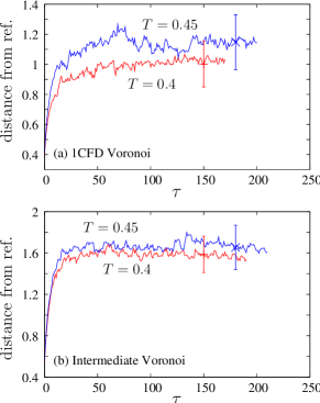
Figure 3: Convergence of trajectories in Voronoi bins as functions of time increment $\tau$. Panel (a) shows, for two different temperatures, the distance of trajectories in the 1CFD bin from the 1CFD structure. Panel (b) shows similar results for an intermediate structure. The spread associated with the trajectories in a bin is also depicted at one specific $\tau$. ($\tau=10000$ MC steps).

Figure 3 shows the convergence of trajectories for two of the regions (1CFD and an intermediate). Clearly, convergence is reached at both the temperatures with increasing time increment, $\tau$. In all the cases, the trajectories within a region spread a substantial distance away from each reference structure, with the effect being more pronounced at higher temperature. Further, the spread of trajectories is greater at the higher temperature.

One important point that emerges from Figure 3 is that time required for equilibration within a bin is similar at the two temperatures. This is due to the use of probability adjustment procedure as described in Section 2.2.1: without the use of such a procedure, it takes significantly more time to equilibrate within a region at a lower temperature (data not shown). This observation of similar equilibration times at the two temperatures has a profound significance: the computational times to obtain steady state rates between two states at the two different temperatures are similar. This is in sharp contrast to brute-force sampling to determine steady state rates.

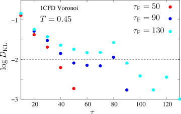
Figure 4: Convergence of transition rates from the 1CFD Voronoi region to other regions as a function of time. KL divergence (eq 3) from the final block (averaged over 10 $\tau$) is compared with the KL divergence from previous blocks. The figure shows such a comparison for three different instances of the final block ($\tau_{\mathrm{F}}$). The reference line for $D_{\mathrm{KL}}=10^{-2}$ is also shown.

Beyond equilibration within a region, we explicitly seek a convergence of transition probabilities between each pair of regions. A measure for this convergence is discussed above in Section 2.2.2. Figure 4 shows $D_{\mathrm{KL}}$ for the trajectories in the 1CFD Voronoi bin for three different instances of the final block averaged values of the transition rates. Clearly, as $D_{\mathrm{KL}}$ is computed after longer times, more and more previous block averages are similar ($D_{\mathrm{KL}}<10^{-2}$) to the corresponding final block averages. For the 1CFD region shown in Figure 4, four previous block averages give transition rates with $D_{\mathrm{KL}}<10^{-2}$ for the green symbols. “Production” transition probabilities are, then, computed for further 60 $\tau$.

The convergence of transition probabilities is robust with regards to block size: when blocks of $20\tau$ are used, identical results are obtained.

4.2 Transition probabilities

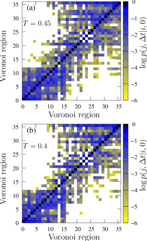
Figure 5: Transition probabilities between each pair of regions – (a) $T=0.45$, and (b) $T=0.4$, for $1\tau=10000$ MC steps.

Equilibrated transition probabilities are key towards computing populations of regions and transition rates between states. The final averaged transition probabilities between regions are shown in Figure 5 for the two temperatures. Two distinct blocks of regions emerge from each panel of Figure 5, indicating a clear two-state decomposition of the sampled conformational space. Further, as expected, the transition probabilities are more diffuse at the higher temperature.

Using these transition probabilities, we, then, compute the population of each region as described in Section 2.4, followed by a combination of regions into a total of two states.

4.3 Populations of regions and combination into states

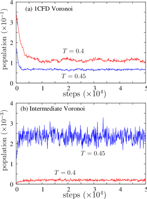
Figure 6: Rapid convergence, at $T=$ 0.45 and 0.4, of fractional population in each state (shown for (a) 1CFD Voronoi region, and (b) an intermediate Voronoi region) upon sequential application of randomly selected stochastic matrices.

Successive multiplications of an arbitrary initial distribution of populations by a stochastic matrix lead to (rapidly) converged estimates of populations of the regions. Since we have a distribution of stochastic matrices (due to estimated errors in the transition probabilities), we obtain fluctuating values of region populations, as shown in Figure 6 for two of the regions. However, since the different estimates of the stochastic matrix are similar (reasonable statistical precision and converged transition probabilities), the distribution of fractional populations around the mean is fairly narrow.

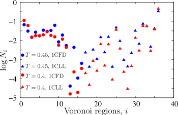
Figure 7: Comparison of fractional populations of different Voronoi regions at two different temperatures. The two extreme regions, $i=1$ and $i=36$ represent 1CFD and 1CLL regions, respectively. Other regions (shown by circles and triangles) belonging to either of the two states (1CFD and 1CLL states) are shown by identical symbols.

Figure 7 shows the averaged populations of different regions for both the temperatures. Clearly, the two end states (regions 1 and 36, corresponding to 1CLL and 1CFD, respectively) show the high populations, whereas intermediate regions far from both 1CLL and 1CFD show low populations. A combination of regions into states, as discussed in Section 2.5.1, leads to the identification of each region with one of the two states (as shown by different symbols, circles and triangles, in Figure 7).

As temperature increases, we expect fractional populations to become more diffuse: population from basins is redistributed into intermediate structures. Clearly, a comparison of populations of each region at the two temperatures in Figure 7 shows that the two end regions show a higher population at the lower temperature, whereas for intermediate regions, the population is higher at the higher temperature.

Another feature that emerges from Figure 7 is the apparent “roughness” of the free energy (negative of the ordinate in Figure 7) surface in the 1CFD state as compared to the 1CLL state. A related feature is that the regions in the two states that are closest to the transition region(s) between the two states show higher populations than regions further inside a state (compare region 16 with region 15, for example), suggesting that the free energy surface shows an apparent local minimum near the transition. However, it is not possible to assert these observations conclusively since the volumes of the Voronoi regions may not be equal.

A summation of populations of regions gives the state populations. At $T=0.45$, the 1CLL state has a fractional population of 0.34. A Similar value (0.35) is obtained at $T=0.4$.

4.4 Transition rates between states

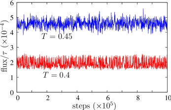
Figure 8: Comparison of fluxes between 1CFD and 1CLL states as a function of sequential random selection of the stochastic transition matrices. The distribution of flux values gives an indication of the confidence region for each flux.

Populations of regions, combination of regions into states, and transition probabilities lead to the computation of transition flux between the two states (cf. Section ). Figure 8 shows the transition fluxes between the two states (symmetric) for the two temperatures. Again, we obtain a distribution of fluxes that are fairly close to the mean values. Further, as expected, the fluxes between the two states are higher at $T=0.45$.

The computed transition rates between the two states are reported in Table 1. Decreasing the temperature from $0.45$ to $0.4$ decreased the transition rate by approximately a factor of 2 in either direction.

5 Discussion

5.1 Efficiency compared to brute–force simulations

The main aim of this manuscript is to present an efficient method to compute transition rates for a two–state system. Thus, in this section, we compare the time required for computing transition rates via this method with an estimate of time required via brute–force simulations.

The total number of Monte Carlo steps required comprise of mainly the time required to establish equilibrium and the time for production runs for transition probabilities in each region (the generation of initial path(s) at elevated temperatures, or via fast network models is a small fraction of this time, and the time for matrix multiplications for computing populations of regions and, subsequently, rates is negligible). Since we use a thousand trajectories in each region, the total number of MC steps are approximately $5\times 10^{10}$, at either temperature.

For establishing equilibrium via brute force throughout the configurational space, there must be several traversals of a trajectory between the two structures. The transition rates (based on MC steps) from the 1CLL structure to the vicinity of 1CFD structure were computed by Zhang et al.²⁴ at $T=0.45$ and $T=0.4$ to be $7\times 10^{-11}$ and $8\times 10^{-12}$, respectively. (We emphasize that these transition rates are from one structure to the vicinity of another structure and not from one state to the other: they cannot be compared directly). The mean first passage times from 1CLL to the vicinity of 1CFD are, thus, $1.4\times 10^{10}$ and $1.3\times 10^{11}$ MC steps at $T=0.45$ and $T=0.4$, respectively. Clearly, if several such passages are required in both directions, brute–force simulations are significantly less efficient than the method discussed in this manuscript. Further, the efficiency of brute-force simulations is dramatically decreased at lower temperatures, in contrast to the method presented.

5.2 Contrast with Markov models and applicability

The method presented here bears some similarities to Markov models^{32, 33} that are used to study transitions between states. However, there is an important distinction. In Markovian analysis, several microstates (similar to regions in the present work) are combined, based on rates between them, to form macrostates. Subsequently, the rates between the macrostates can be computed based on rates (or, transition probabilities) between the microstates. The combination into Markovian macrostates allows one to consider only the rates between states, and not the equilibration within a state.

In contrast, the use of the equivalence between steady–state flux and the mean first passage rate in the current work allows for the relaxation of the Markovian condition. Instead, the computed rates by the current method are steady–state rates for the situation when steady state is established by feeding the trajectories that enter into the target state immediately back into the starting state (and the feedback is such that the equilibrium distribution in the initial state is maintained). Thus, in effect, the computed rates are equilibrium rates between the two states.

Two aspects emerge from the preceding discussion - both due to the equivalence of steady–state flux and mean first passage rate. First, the feedback must be immediate for this relation to be exactly valid. In contrast, $\tau\equiv\Delta t=10000$ MC steps above. However, if the two states are separated by a barrier, any trajectories that enter a different state between two updates, separated by $\tau$, are unlikely to escape the new state during a $\tau$ interval. Thus, we expect that relation to be valid for range of $\tau$. We emphasize that the presence of such a barrier does not necessarily imply that either state behaves in a Markovian fashion within the $\tau$ interval: the time for equilibration within either state may be significantly more than $\tau$ without affecting the validity of the current approach.

The second aspect is that the explicit use of the equivalence restricts the use of the approach to two–state problems. However, as mentioned in the Introduction, such two–state problems are encountered very frequently.

6 Conclusions

In this manuscript, we present a method to compute transition rates between states for two–state systems that are frequently encountered in enzyme kinetics and protein–folding studies. The crucial idea we employ is the equivalence between steady–state flux and the mean first passage transition rate, and that the division of the configurational space into smaller regions allows for a faster equilibration within a region. We find that an adaptive enhancement procedure greatly facilitates equilibration within a region, allowing for an efficient computation of conditional transition probabilities between regions. Further, this adaptive enhancement procedure is not substantially affected by a decrease in temperature, making the procedure increasingly efficient (when compared to brute–force simulations) as the temperature is decreased. This leads to an efficient calculation of state populations and transition rates even as the temperature is decreased.

Figure 1: A schematic of division of the relevant configuration space into Voronoi regions (e.g., any point inside region $i$ is closer to the structure defining region $i$ (represented by a solid circle) than to the structure defining any other region. Two such regions are explicitly labeled with transition probabilities between them depicted.

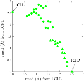
Figure 2: Structures used to construct Voronoi bins along a putative transition pathway between the two crystal structures of calmodulin (1CLL and 1CFD) plotted as rmsd from the two structures. The circles represent structures that are closer to 1CLL, whereas the triangles represent structures closer to 1CFD. The two known crystal structures (1CFD and 1CLL) are also shown labeled.

Table 1: Transition rates between the two states.

$T$	1CLL to 1CFD (/MC step)	1CFD to 1CLL (/MC step)
0.45	$1.3\times 10^{-7}$	$7.0\times 10^{-8}$
0.4	$5.5\times 10^{-8}$	$3.0\times 10^{-8}$

References

- 1 Hammes, G. G., Y.-C. Chang, and T. G. Oas. 2009. Conformational selection or induced fit: A flux description of reaction mechanism. Proc. Natl. Acad. Sci. 106:13737–13741.
- 2 Weikl, T. R., and C. von Deuster. 2009. Selected-fit versus induced-fit protein binding: Kinetic differences and mutational analysis. Proteins. 75:104–110.
- 3 Hanson, J. A., K. Duderstadt, L. P. Watkins, S. Bhattacharyya, J. Brokaw, and J.-W. Chu. 104. Illuminating the mechanistic roles of enzyme conformational dynamics. Proc. Natl. Acad. Sci. 46:18055–18060.
- 4 Schlitter, J., M. Engels, P. Kruger, E. Jacoby, and A. Wollmer. 1993. Targeted molecular–dynamics simulation of conformational change – application to the t–r transition in insulin. Mol. Simul. 10:291–309.
- 5 Ma, J., and M. Karplus. 1997. Molecular switch in signal transduction: Reaction paths of the conformational changes in ras p21. Proc. Natl. Acad. Sci. 94:11905–11910.
- 6 Apostolakis, J., P. Ferrara, and A. Caflisch. 1999. Calculation of conformational transitions and barriers in solvated systems: Application to alanine dipeptide in water. J. Chem. Phys. 110:2099–2108.
- 7 Elber, R. 1987. A method for determining reaction paths in large molecules – application to myoglobin. Chem. Phys. Lett. 139:375.
- 8 Ulitsky, A. 1990. A new technique to calculate steepest descent paths in flexible polyatomic systems. J. Chem. Phys. 92:1519.
- 9 Fischer, S., and M. Karplus. 1992. Conjugate peak refinement – an algorithm for finding reaction paths and accurate transition states in systems with many degrees of freedom. Chem. Phys. Lett. 194:252.
- 10 Sevick, E. M., A. T. Bell, and D. N. Theodorou. 1993. A chain of states method for investigating infrequent event processes occurring in multistate, multidimensional systems. J. Chem. Phys. 98:3196.
- 11 Gillilan, R. E., and K. R. Wilson. 1992. Shadowing, rare events, and rubber bands – a variational verlet algorithm for molecular dynamics. J. Chem. Phys. 97:1757.
- 12 Elber, R., A. Ghosh, A. Cardenas, and H. Stern. 2004. Bridging the gap between long time trajectories and reaction pathways. Adv. Chem. Phys. 126:123.
- 13 Passerone, D., M. Ceccarelli, and M. Parrinello. 2003. A concerted variational strategy for investigating rare events. J. Chem. Phys. 118:2025.
- 14 Olender, R., and R. Elber. 1996. Calculation of classical trajectories witha very large time step: Formalism and numerical examples. J. Chem. Phys. 105:9299.
- 15 Pan, A. C., D. Sezer, and B. Roux. 2008. Finding transition pathways using the string method with swarms of trajectories. J. Phys. Chem. B. 112:3432–3440.
- 16 Temiz, N. A., E. Meirovitch, and I. Bahar. 2004. Escherichia coli adenylate kinase dynamics: Comparison of elastic network model modes with mode-coupling n-15-nmr relaxation data. Prot. Struct. Func. Bioinfor. 57:468–480.
- 17 Maragakis, P., and M. Karplus. 2005. Large amplitude conformational change in proteins explored with a plastic network model: Adenylate kinase. J. Mol. Biol. 352:807–822.
- 18 Whitford, P. C., O. Miyashita, Y. Levy, and J. N. Onuchic. 2007. Conformational transitions of adenylate kinase: Switching by cracking. J. Mol. Biol. 366:1661–1671.
- 19 Chennubhotla, C., and I. Bahar. 2007. Signal propagation in proteins and relation to equilibrium fluctuations. PLoS Comput. Biol. 3:1716–1726.
- 20 Chu, J. W., and G. A. Voth. 2007. Coarse-grained free energy functions for studying protein conformational changes: A double-well network model. Biophys. J. 93:3860–3871.
- 21 Yang, Z., P. Majek, and I. Bahar. 2009. Allosteric transitions of supramolecular systems explored by network models: Application to chaperonin groel. PLOS Comp. Biol. 5:e1000360.
- 22 Hill, T. L. 1989. Free Energy Transduction and Biochemical Cycle Kinetics. Dover Publications, New York.
- 23 Bhatt, D., B. W. Zhang, and D. Zuckerman. 2010. Steady–state simulations using weighted ensemble path sampling. J. Chem. Phys. 133:014110.
- 24 Zhang, B. W., D. Jasnow, and D. M. Zuckerman. 2007. Efficient and verified simulation of a path ensemble for conformational change in a united-residue model of calmodulin. Proc. Natl. Acad. Sci. 104:18043–18048.
- 25 Huber, G. A., and S. Kim. 1996. Weighted–ensemble brownian dynamics simulations for protein association reactions. Biophys. J. 70:97–110.
- 26 Kullback, S., and R. A. Leibler. 1951. On information and sufficiency. Ann. Math. Stat. 22:79–86.
- 27 Bhatt, D., and D. M. Zuckerman. 2011. Beyond microscopic reversibility: Are observable nonequilibrium processes precisely reversible? J. Chem. Theory Comput. :ASAP.
- 28 Zuckerman, D. M. 2004. Simulation of an ensemble of conformational transitions in a united–residue model of calmodulin. J. Phys. Chem. B. 108:5127–5137.
- 29 Best, R. B., Y.-G. Chen, and G. Hummer. 2005. Slow protein conformational dynamics from multiple experimental structures: The helix/sheet transition of arc repressor. Struct. 13:1755–1763.
- 30 Levy, Y., S. S. Cho, T. Shen, J. N. Onuchic, and P. G. Wolynes. 2005. Symmetry and frustration in protein energy landscapes: A near degeneracy resolves the rop dimer-folding mystery. Proc. Natl. Acad. Sci. 102:2373–2378.
- 31 Metropolis, N., A. W. Rosenbluth, M. N. Rosenbluth, A. H. Teller, and E. Teller. 1953. Equation of state calculations by fast computing machines. J. Chem. Phys. 21:1087–1092.
- 32 Ozkan, S. B., K. A. Dill, and I. Bahar. 2002. Fast-folding protein kinetics, hidden intermediates and the sequential stabilization model. Protein Sci. 11:1958–1970.
- 33 Chodera, J. D., N. Singhal, W. C. Swope, V. S. Pande, and K. A. Dill. 2007. Automatic discovery of metastable states for the construction of markov models of macromolecular conformational dynamics. J. Chem. Phys. 126:155101.