Inserting physics associated with the transverse polarization of the quarks into a standard Monte Carlo generator, without touching the code itself.

Abstract

The transverse polarization of a quark is a degree of freedom that is not taken into account in the most commonly used Monte Carlo generators. For the case $e^{+}e^{-}$ $\rightarrow$ $hadrons$ I show that it is possible to use these generators to simulate processes where the parent quark and antiquark are transversely polarized and the fragmentation process is affected by this polarization. The key point is that it is possible to obtain this without touching the generator code at all. One only works on the parton-level and hadron-level outputs that the Monte Carlo code has produced, modifying them in a correlated way. A group of techniques is presented to obtain this, matching the most obvious needs of a user (in particular: reproducing a pre-assigned final distribution). As an example these methods are applied to modify Pythia-generated events to obtain a nonzero Collins function and a consequent $cos(\Phi_{1}+\Phi_{2})-$asymmetry of pion pairs.

1 Introduction

A great effort covering several decades has been devoted to developing full-purpose MonteCarlo codes (e.g. [1, 2, 3], see [4] for a more general review) for high-energy hard processes. However, the most known codes do not allow for simulation of effects like azimuthal asymmetries in SIDIS, in $e^{+}e^{-}$ $\rightarrow$ hadrons, in Drell-Yan processes etc, i.e. those processes where the transverse spin of the quark has a relevance (for an overview of this field, see the proceedings [5], and the reviews [6] and [7]).

Although it is possible to modify a Monte Carlo generator in such a way to produce such asymmetries, the perspective of touching the core of such complicate codes is surely a nightmare for most of the people that are potentially interested in. What I present here is a set of techniques aimed at introducing (transverse) spin physics in a generator without touching it at all. Of course one needs writing patches of code, but these use the parton level and hadron level outputs of the generator as an input, and are completely independent (small) programs.

In this work, I will consider $e^{+}e^{-}$ $\rightarrow$ hadrons. I will start from events generated by Pythia-8 [1]. I need to modify Pythia outputs in such a way that:

(i) In the hard vertex $e^{+}e^{-}$ $\rightarrow$ $q\bar{q}$, transverse polarizations are added to the quark and to the antiquark, and the correlated distribution of spins and momenta is coherent with the known matrix elements.

(ii) The momenta of the final hadrons in each hemisphere (quark hemisphere and antiquark hemisphere) are modified in a way that is correlated with the transverse spin of the parent quark. The modification must be under our full control, i.e. we should be able to obtain exactly what we want to obtain. This may mean a fragmentation function with pre-assigned form, or the implementation of a model.

I will describe some techniques to implement the previous requirements. As an example, I will apply them to modify pion final momenta so to have them distributed according with the sum of an unpolarized and a Collins fragmentation function[8]. Although here I just want to show an example of application of these simulation techniques, the chosen case is of special interest, since the Collins function has a relevant role in the extraction of information on the transverse polarization of the nucleon[9], there are models for it [10, 11, 12], and it appears in asymmetries measured in SIDIS [13, 14, 15] and $e+e^{-}$ $\rightarrow$ $hadrons$ [18].

As a consequence of a nonzero Collins function, the correlated distribution of pions detected in opposite hemispheres is expected to present a $cos(\Phi_{1}+\Phi_{2})$ asymmetry in the sum of the azimuthal angles of the pions [16] (see section VIII of [17] for details). This will be confirmed by an analysis of the events generated by Pythia and modified as suggested here.

I will not try to reproduce the detailed physical outputs of the recent measurement of this quantity at Belle [18, 19], because this is just an exercise and the aim of this work is to present a more general group of techniques. Once the individual hadron tracks have been modified in a physically motivated way, other azimuthal asymmetries could be generated in a set of simulated events, like the $cos(2\phi)-$asymmetry (see [17] and [19]), or dihadron-dihadron correlations [20, 21], or even asymmetries associated with a larger number of particles[22].

Let me name NPMC the “non polarized” MonteCarlo code whose outputs have to be modified by the external patches.

The two main steps, corresponding to previous (i) and (ii) are:

Step (1): Take a $q\bar{q}$ pair produced in the hard vertex by the NPMC and “stick” a pair of reciprocally independent random transverse spins, in such a way that the correlated spin-momentum distribution agrees with the polarized quark-lepton squared matrix element. Transverse spins are assumed to be classical fixed-length vectors with one degree of freedom (the angle in the plane that is normal to the quark momentum).

This step is the critical point of the method. It needs to be demonstrated that it is feasible. One thing is to sort both momenta and spins according with a joint distribution, and another thing is first sorting momenta according with the spin-averaged distribution (that is done by the NPMC), and next dividing the sorted events into fairly distributed spin subsets (that is done by us). Section 2 is devoted to this.

Step (2): Modify the (final or intermediate) hadronic momenta so to reproduce the effect of an assigned quark-spin-dependent fragmentation function. Alternatively, one could like to implement a physical model that is behind this fragmentation function.

Here the underlying assumption is that azimuthal effects are a $small$ distortion of a final particle distribution that is mainly determined by the physics implemented in the NPMC. There are two classes of techniques that may be exploited: “distortion”, and “filtering” techniques. In distortion techniques the individual particle properties in a given event are modified. These techniques exploit each event produced by the NPMC. In filtering techniques only a subset of the events produced by the NPMC is accepted.

Filtering may be expensive, when many NPMC-events are needed to obtain one final event. It may be necessary when we think that the additional physical processes affect quantities like the final pion multiplicity, or the general structure of the event. If we do not expect this to be the case, distortion techniques are preferable.

In section 3, I show the effect of two possible distortion techniques in producing a nonzero Collins function for the pions.

A $cos(\Phi_{1}+\Phi_{2})-$asymmetry involving pions of the opposite hemispheres is a synthesis of the presence of Collins functions on both sides, and of the spin correlations between the quark and antiquark produced in the hard vertex. So, if things in the steps (1) and (2) have been properly performed it must be present. Section 4 is devoted to show that this is the case, i.e. that a $cos(\Phi_{1}+\Phi_{2})-$asymmetry is present in a set of Pythia-events modified by the presented techniques.

2 Step 1: Hard vertex and spin

In most MonteCarlo codes for high-energy physics, the starting point is the hard scattering process at parton level. Once a hard scattering event has been sorted according with some probability, both later and previous cascading processes are generated.

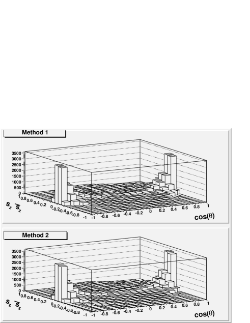
Figure 1: Event distribution as a function of the quark-lepton angle $\theta$ and of the components of spins of the quark and antiquark along the lepton axis.

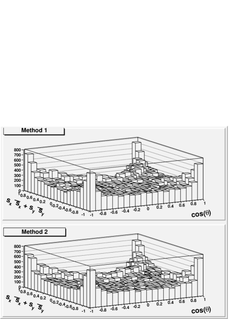
Figure 2: Event distribution as a function of the quark-lepton angle $\theta$ and of the components of spins of the quark and antiquark on the plane normal to the lepton axis (see the next figure for the individual contributions of $x$ and $y$ terms).

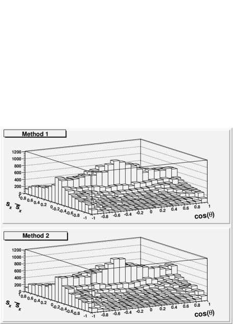
Figure 3: Event distribution as a function of the quark-lepton angle $\theta$ and of the components of spins of the quark and antiquark along the $x-$axis (the corresponding $y-$distribution is equal).

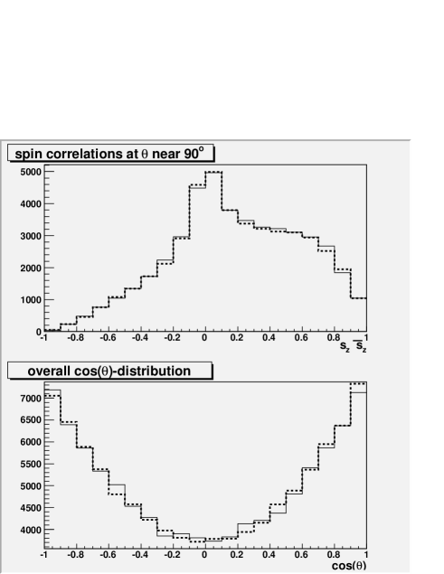
Figure 4: Upper panel: $s_{z}\bar{s}_{z}-$distribution integrated over the $cos(\theta)-$range $(-0.5,0.5)$. Lower panel: the $cos(\theta)-$distribution, summed over spins. The continuous line is obtained with Method 1, the dotted line with Method 2.

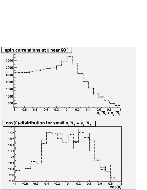
Figure 5: Upper panel: $s_{x}\bar{s}_{x}+s_{y}\bar{s}_{y}-$distribution integrated over the $cos(\theta)-$range $(-0.5,0.5)$. Lower panel: the $cos(\theta-)$distribution, for $-0.2$ $<$ $s_{x}\bar{s}_{x}+s_{y}\bar{s}_{y}$ $<$ $0.2$. The continuous line is obtained with Method 1, the dotted line with Method 2.

In the case of $e^{+}e^{-}$ $\rightarrow$ $hadrons$, the (parton level) cross section for the hard scattering process $e^{+}e^{-}$ $\rightarrow$ $q\bar{q}$ with transversely-polarized quarks, and with the leptons on the $z-$ axis, is (see Appendix):

$$W_{pol}(\hat{N},\vec{s},\vec{\bar{s}})\ =\ {1\over 4}\Bigg{(}[1\ +\ cos^{2}(\theta)](1\ +\ s_{z}\bar{s}_{z})\$$

$$-\ sin^{2}(\theta)(s_{x}\bar{s}_{x}\ +\ s_{y}\bar{s}_{y})\Bigg{)}$$ (1)

where $\hat{N}$ is a versor of the quark momentum ($-\vec{N}$ is the corresponding one for the antiquark), $\theta$ is the angle between the lepton and quark axes ($cos(\theta)$ $=$ $\hat{N}\cdot\hat{z}$) and $\vec{s}$, $\vec{\bar{s}}$ are transverse polarization vectors. “Transverse” means “transverse to the (anti)quark 3-momenta”. Since the quark momentum is not aligned with the electron momentum, the transverse spin has a nonzero $s_{z}$ component, i.e. a component along the electron-positron beam axis. This must not be confused with the helicity or with the longitudinal spin of the quark.

This cross section was already reported in [23] where it was applied to the Drell-Yan process in the context of the Panda experiment[24]. The two cross sections present a different form because they are expressed in different reference frames, but they are the same.

If the polarization components are averaged away, we get the known result

$$W_{nopol}(\hat{N})\ \propto\ 1\ +\ cos^{2}(\theta).$$ (2)

The most known and used MonteCarlo codes implement this equation for the lepton-quark vertex, adding further $O(\alpha_{s}^{n})$ hard processes in the partonic showers.

If we had to write from the very beginning a complete MonteCarlo generator including transverse polarizations of the quark and antiquark, we could imagine two ways of sorting momenta $and$ spins of the quark and of the antiquark (generically: “quarks”).

Method 1) The momenta and the spins of the quarks are jointly sorted according with the probability law eq.1.

Method 2) First, the momenta of the quarks are sorted accordingly with eq.2, and next the polarizations are sorted in such a way to get the distribution 1 for the joint set of variables $\hat{N},\vec{s},\vec{\bar{s}}$.

The former one is the right one in general (if correctly implemented). The latter method allows for splitting the generation process into two steps, one of which may be performed by an NPMC and the other one by our additional code patches. I will show that in the case interesting us it produces the same results of method 1.

To apply Method 2 here I take a quark-antiquark pair whose momenta have been sorted with probability $W_{nopol}(\hat{N})$, and sort their spins according with the distribution

$$D(\hat{N},\vec{s},\vec{\bar{s}})\ =\ {{W_{pol}(\hat{N},\vec{s},\vec{\bar{s}})}\over{W_{nopol}(\hat{N})}}\ \rightarrow\ W_{pol}(\hat{N},\vec{s},\vec{\bar{s}})$$ (3)

subject to the conditions

$$\vec{s}\cdot\hat{N}=\vec{\bar{s}}\cdot\hat{N}\ =\ 0,$$

$$|\vec{s}|\ =\ 1,\ |\vec{\bar{s}}|\ =\ 1.$$ (4)

In eq.3, in general, $D$ requires the denominator $W_{nopol}$. In this peculiar case it may be removed since we sort a variable that is absent in this denominator.

For method 1 the implementation is more straightforward. Events are sorted according with the probability distribution eq. 1, subject to the condition 4.

In the set of figures 1$-$5 the distributions of some variables and of their correlations are reported, calculated with both Method 1 and 2. These show that Method 1 and 2 produce the same results.

Since the full distribution shows a strong correlation between $\theta$ and $s_{z}\bar{s}_{z}$ on one side, and between $\theta$ and $s_{x}\bar{s}_{x}+s_{y}\bar{s}_{y}$ on the other side, the scatter plot of these pairs of variables is shown in figs. 1-2. These figures report the distribution of 100,000 events in the $(cos\theta,A)-$plane, where $A$ is $s_{z}\bar{s}_{z}$ (fig.1), $s_{x}\bar{s}_{x}+s_{y}\bar{s}_{y}$ (fig.2), $s_{x}\bar{s}_{x}$ (fig.3).

The other figures show slices/integrals of the previous distributions. In fig.4 (upper panel) I report the $s_{z}\bar{s}_{z}$-distribution integrated over $-0.5$ $<$ $cos(\theta)$ $<$ $0.5$. This region is relevant for the Collins effect that is suppressed for $|cos(\theta)|$ near 1. In the lower panel the spin-integrated $cos(\theta)-$distribution is reported. It reproduces the $1+cos^{2}(\theta)$ shape within 5 %. In fig.5 (upper panel) I report the distribution of $s_{x}\bar{s}_{x}+s_{y}\bar{s}_{y}$ integrated over $-0.5$ $<$ $cos\theta)$ $<$ $0.5$. In the lower panel the distribution is the one of $cos(\theta)$ for the integration range $-0.2$ $<$ $s_{x}\bar{s}_{x}+s_{y}\bar{s}_{y}$ $<$ $0.2$. In the last case, the larger (fluctuating) discrepancies between the distributions obtained by the two methods have statistical origin, and are due to the relatively small number of events in each bin.

Concluding this part, I may claim that Methods 1 and 2 give similar results, so it is licit to apply the polarization stage of method 2 to events sorted by some independent generator that does not include spins.

3 Step 2: Reasonable choices for the distortion methods

Now we need to modify the transverse momenta of the final hadrons in such a way to reproduce an assigned distribution, that is correlated with the quark polarization. In an attempt to be as comprehensive as possible, I propose and test two classes of methods, that I name “product” and “convolution”. These should fit the most obvious requirements.

In this section, I apply these methods to a set of 2-momenta that are gaussian-distributed in the $xy-$plane with center of the distribution in the origin. They are supposed to be the transverse momenta of a set of final hadrons, originating from a parent quark that is directed along $+\hat{z}$ and has polarization $+\hat{x}$. After testing the distorting methods on this simplified set, in the next section they will be applied to a set of Pythia events.

Let $F_{0}(K_{T})$ be the undistorted momentum distribution, that depends on $\vec{K}_{T}$ via $|\vec{K}_{T}|$ only. It depends on the longitudinal fraction $Z$ (not explicitly reported) and is proportional to the fragmentation function $D_{1}(q\rightarrow h;Z,K_{T})$, where $q$ is one or a group of quark flavors and $h$ is one or a group of hadron species. $F_{0}$ is normalized to 1, while $D_{1}$ is normalized to the total hadron multiplicity in the subset of events $q$ $\rightarrow$ $h$.

Let $G(\vec{K}_{T})$ be a distorting factor, that introduces azimuthal asymmetries in the $xy-$plane. It may depend on $Z$, but I do not write this explicitly.

Product techniques: the final distribution has the form

$$F(\vec{K}_{T})\ =\ F_{0}(K_{T})\ G(\vec{K}_{T}).$$ (5)

Convolution techniques: the final distribution has the form

$$F(\vec{K}_{T})\ =\ \int d\vec{k}_{T}d\vec{q}_{T}\delta(\vec{K}_{T}\ -\ \vec{k}_{T}\ -\ \vec{q}_{T})\ F_{0}(K_{T})\ G(\vec{q}_{T}).$$ (6)

or, more in general,

$$F(\vec{K}_{T})\ =\ \int d\vec{k}_{T}d\vec{q}_{T}\delta(\vec{K}_{T}\ -\ \vec{k}_{T}\ -\ \vec{q}_{T})$$

$$\ F_{0}(K_{T})\ G(\vec{K}_{T},\vec{q}_{T}).$$ (7)

The latter form is not strictly a convolution, but I will use this name anyway. Sometimes, a starting model suggests a form like in eq.6, but some constraint on $\vec{K}_{T}+\vec{q}_{T}$ (when sorting $\vec{q}_{T}$) may remove the full independence of $G(\vec{q}_{T})$ from $K_{T}$.

The product form allows an easy implementation of parametrizations of the form

$$D_{1}(z.K_{T})\ \Big{(}1\ +\ {{H(z,\vec{K}_{T})}\over{D_{1}(z,K_{T})}}\Big{)}.$$ (8)

The convolution form is more flexible to implement physical models, since it treats the final hadron momentum as a sum of momenta with independent physical origin.

3.1 Implementation: the product case

To implement the product form I have chosen an algorithm belonging to the Metropolis-Hastings family [25, 26]:

1) I start with an “undistorted” event $\vec{K}_{T}$.

2) A shift $\vec{q}_{T}$ is sorted (flat distribution) inside a circle of radius $R_{q}$.

3) The “shift probability” is

$$P(\vec{K}_{T},\vec{K}_{T}+\vec{q}_{T})\ \equiv\ {{F(\vec{K}_{T}+\vec{q}_{T})}\over{F(\vec{K}_{T})}}$$ (9)

If this quantity is $>$ $1$, the step to the new point $\vec{K}_{T}+\vec{q}_{T}$ is performed. If it is not, an accept/reject procedure is set. As a consequence, with probability $P(\vec{K}_{T},\vec{K}_{T}+\vec{q}_{T})$ the step is performed, and with probability $1-P(\vec{K}_{T},\vec{K}_{T}+\vec{q}_{T})$ the step is not performed.

4) As a result, we have a new point $\vec{K}_{T}^{\prime}$ that either coincides with $\vec{K}_{T}$ or with $\vec{K}_{T}+\vec{q}_{T}$.

5) The sequence 2-4 is repeated starting with the value $\vec{K}_{T}^{\prime}$ instead of $\vec{K}_{T}$. A new point $\vec{K}_{T}^{\prime\prime}$ is selected.

6) The sequence 2-4 may be performed $N$ times.

Comments:

For $N$ $=$ 1 and for a small admitted displacement $\vec{q}_{T}$ the final distribution is similar to the starting one $F_{0}(K_{T})$.

For $N$ $=$ 10 the final distribution coincides with $F(\vec{K}_{T})$ whichever the starting distribution was (e.g. one may choose $\vec{K}_{T}$ $=$ 0 fixed). So the joint choice of $N$ and $F_{0}(K_{T})$ must be clever, in those cases where one does not know precisely the distribution of the undistorted events.

3.2 Implementation: the convolution case

The implementation of the convolution method is more straightforward. In general terms, to get a distribution of the form $h(X)$ $\equiv$ $\int dx\int dyf(x)g(y)\delta(X-x-y)$ the steps are

1) Sort $x$ according with $f(x)$.

2) Sort $y$ according with $g(y)$.

3) Sum $x$ and $y$.

This may work to produce both a distribution of the form eq. 6, and one of the form eq. 7.

3.3 The examples of fig.6

As an example I have chosen, both for the undistorted distribution, and for the distortion factors, some shapes that simplify much the computational work (in particular, imposing that the distorting factors are zero in some parts of the phase space). Apart for this, they do not present any special lack of generality.

In the examples of fig.6, as an undistorted and axially symmetric distribution $F_{0}(K_{T})$ I have chosen the gaussian

$$F_{0}(K_{T})\ =\ exp[-(K_{x}^{2}+K_{y}^{2})/(2k_{1}^{2})]$$ (10)

with $k_{1}$ $=$ 0.5 GeV/c.

For the product case I have applied eq. 5 with

$$G(\vec{K}_{T})\ =\$$

$$\bigg{(}1\ +\ \alpha K_{y}exp[-(K_{x}^{2}+K_{y}^{2})/(2k_{2}^{2})]\bigg{)}$$

when this expression is $>$ 0, and

(11)

$$G(\vec{K}_{T})\ =\ 0.$$

(12)

when it is negative.

For the example in fig.6 $\alpha$ $=$ 0.75 and $k_{2}$ $=$ 4 GeV/c $>>$ $k_{1}$. At any step, the shift $\vec{q}_{T}$ is sorted with $q_{x}$ $=$ 0 and $|q_{y}|$ $<$ 1 GeV/c. I have used $N$ $=$ 10 steps, but already with 5 steps the final results converges towards the final required distribution.

For the convolution case I have used

$$G(\vec{q}_{T})\ =\ \alpha\ q_{y}\ exp[-(q_{x}^{2}+q_{y}^{2})/(2k_{3}^{2})]\ for\ q_{y}\ >\ 0,$$

$$G(\vec{q}_{T})\ =\ 0\ for\ q_{y}\ <\ 0.$$

(13)

with $\alpha$ $=$ 0.5 and $k_{3}$ $=$ 0.1 GeV/c. These parameters are chosen so that the convolution produces a shift that is similar to the product case. The choices $k_{2}$ $>>$ $k_{1}$ (product case), and $k_{3}$ $<<$ $k_{1}$ (convolution case) lead to a similar result, i.e. avoiding that the final distribution is much broader than the starting one. This permits us to appreciate the shifting effect, that in fig. 6 is highlighted by vertical lines showing the average point of each distribution.

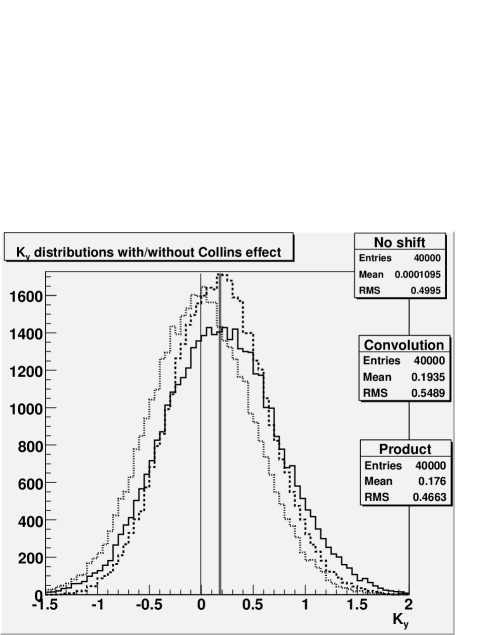
Figure 6: Distribution of 40,000 events obtained by sorting a gaussian distribution w.r.t. $\vec{k}_{T}$ (fine-dotted curve), and next by shifting events according to either the convolution method (continuous) or the product method (coarse-dotted). Vertical lines show the average point of each distribution (the two averages of the shifted events practically overlap).

4 Example: A $cos(\Phi_{1}+\Phi_{2})-$asymmetry in the complete event

As an example, the two described track-distortion methods, with the same parameters as in fig.6 are applied to produce a $cos(\Phi_{1}+\Phi_{2})$ nonzero term in the distribution of pion pairs generated by Pythia in the conditions of the Belle experiment in the sub-$b\bar{b}$ energy range, at $Q$ $=$ 10.0 GeV (Belle has performed measurements in this range, and at a slightly higher $Q$ at the $b\bar{b}$ threshold[19]).

To apply the previous methods to events produced by Pythia some further complications are needed. I do not give details on these points since they just require standard operations like frame rotations and vector projections. What is done is (1) the distortion of the hadron transverse momentum is produced in a frame where the parent quark (or antiquark) momentum and spin are along the $z$ and $x$ axes (this reproduces the situation analyzed in the previous section), (2) for the specific data analysis (i.e. extraction of the $cos(\Phi_{1}+\Phi_{2})-$distribution) each resulting hadron momentum is transferred to a frame where the lepton-quark scattering plane coincides with the a coordinate plane.

The Pythia-generated events are selected by the additional condition Thrust $>$ 0.8. This excludes three-jet events, and in the case of $Q$ slightly over 10 GeV (i.e. over the value used here) it would exclude events of $b\bar{b}-$kind (see the discussion in [19]). This cutoff is important, because the momentum-spin correlation calculated in the Appendix of the present work refers to “light” quarks, i.e. fermions for which it is licit to assume helicity conservation in the vector-fermion vertex. At $Q$ $=$ 10 GeV we have to include events starting from $u\bar{u}$, $d\bar{d}$ $s\bar{s}$ and $c\bar{c}$ pairs. In the collision c.m. frame, the quark energy is 5 GeV. The charm mass is $\approx$ 1.27 GeV/c². For this quark the first order correction to the UR relation $E$ $=$ $P$ is $m^{2}/2E$ $\approx$ 160 MeV $<<$ $E$, so the helicity nonconserving terms have small relevance. If gluon radiation processes with a large $p_{T}$ were included in the hard photon-quark vertex, the spin-momentum correlations would not be exactly as in eq. 1 (e.g. the quark momentum would be modified by a non-collinear gluon radiation, and the large quark virtuality would affect helicity conservation in the photon vertex). All these processes are excluded by the request Thrust $>$ 0.8.

According with e.g. [17] in presence of nonzero Collins functions on both sides one expects a cross section of the form

$${{d\sigma}\over{dz_{1}dz_{2}d\Omega_{1}d\Omega_{2}}}\ \propto\ \Big{[}1\ +\ cos^{2}(\theta)\Big{]}D(z_{1})D(z_{2})\$$

$$+\ sin(\theta)cos(\Phi_{1}+\Phi_{2})C(z_{1})C(z_{2}).$$ (14)

The angle $\theta$ is the lepton-quark polar angle. $\Phi_{1,2}$ are the angles of the pion transverse momenta w.r.t. the lepton-quark scattering plane. $D(z_{1,2})$ and $C(z_{1,2})$ are the unpolarized and Collins fragmentation functions with opposite hemisphere pions with longitudinal fractions $z_{1}$ and $z_{2}$.

Since this is just an example of application, I have not attempted reproducing the recently measured values for this quantity at Belle[18, 19]. Rather, I have reported the output corresponding to the distribution shifts reported in fig.6, including the “no-shift” case to have an estimator of the fake asymmetries due to the statistics and to the cutoffs.

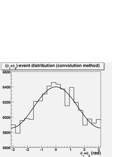
Figure 7: Distribution of the angle $\Phi_{1}+\Phi_{2}$, where the angles $\Phi_{i}$ are the azimuthal angles (see text) of two opposite-hemisphere pions. The individual pion tracks are deflected according with the convolution method. The fitting curve is $\propto$ $1+A\ cos(\Phi_{1}+\Phi_{2})$, with $A$ $=$ 0.04 $\pm$ 0.004.

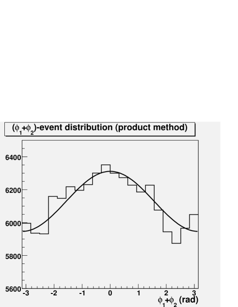
Figure 8: Distribution of the angle $\Phi_{1}+\Phi_{2}$, as in fig.7. The individual pion tracks are here deflected according with the product method. The fitting curve is $\propto$ $1+A\ cos(\Phi_{1}+\Phi_{2})$, with $A$ $=$ 0.03 $\pm$ 0.004.

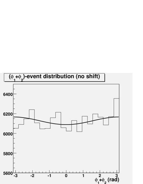
Figure 9: Distribution of the angle $\Phi_{1}+\Phi_{2}$, as in fig.7. The individual pion tracks are not deflected at all, i.e. they are the original trajectories as simulated by Pythia. The fitting curve is $\propto$ $1+A\ cos(\Phi_{1}+\Phi_{2})$, with $A$ $=$ $-$0.006 $\pm$ 0.004.

The three figures 7, 8, 9 show the distribution of 135,000 pion pairs vs $cos(\Phi_{1}+\Phi_{2})$ in Belle conditions. Each event has Thrust $>$ 0.8, and each individual pion has $z$ $>$ 0.1, and $cos(\alpha$ $>$ 0.8, where $\alpha$ is the angle w.r.t. the quark axis (in an attempt of precisely fitting the experimental data, one should include further cuts and use the Thrust axis instead of the quark axis). A “pair” is composed of two pions (regardless of their charge) belonging to different hemispheres.

The produced histograms have been fitted by the Root-Migrad package[27] with curves of the form $B[1+A\ cos(\Phi_{1}+\Phi_{2})]$. The data are divided into 40 equal-range bins, and $B$ $=$ 6130 $\pm$ 20 is the average number of events per bin. $A$ has size 3-4 %, compared to a statistical error 0.4 % and to a zero-asymmetry value 0.6 % (extracted from the last figure, where no azimuthal effect is included).

The chosen form of the spin-dependent fragmentation functions is aimed at simplifying the implementation of the presented examples. I have not considered a dependence of the azimuthal effects on the longitudinal fractions. I have not considered the flavor dependence of the spin-dependent fragmentation functions. I have only considered spin effects on pions. To include different functional forms, a dependence on $z$, flavor differentiation, azimuthal effects on other hadron species (like kaons), would be a matter of more program lines, but would not issue any further challenge.

The same procedure could have been applied to an intermediate state hadron that decayed into two hadrons like e.g. a $\rho$. Then the two decay hadrons would present an extra fragmentation function of the kind $H_{\perp}$ (see [28], [29]). On the other side, to produce a function of the kind $H^{<}$ ([28], [29], in $e^{+}e^{-}$ $\rightarrow$ $hadrons$ it has been measured by [30]) modifications should be applied to the $relative$ momentum of the two final hadrons. These are straightforward generalizations of the work presented here. Another possible application is the production of polarized $\Lambda/\bar{\Lambda}$ [31]. In this case one would sort a spin for this hadron correlated with the quark spin, and sort new momenta for the decay products according with the assigned spin.

5 Conclusions

I have started this work from events of the class $e^{+}e^{-}$ $\rightarrow$ $hadrons$, generated by an ordinary Monte Carlo code where the transverse polarizations of the quarks are not taken into account.

A set of techniques have been presented to build code patches that do not touch the Monte Carlo generator itself, but rather modify its outputs, both at parton and hadron level.

The first aim of these modifications is attributing a transverse spin to the quark and to the antiquark pair produced in the hard vertex, in such a way to get a physically sound distribution for the correlated set of quark momenta and spins produced in the hard vertex. To reach this, $e^{+}e^{-}$ events with production of polarized quarks have been generated according to a known and general method. Next, an alternative two-step method for generating similar events has been tested, where in the first step an unpolarized quark and an unpolarized antiquark are produced in the lepton annihilation, and in the second step both are polarized without touching the previously sorted momenta. I have shown that the two methods produce the same distributions. This means that it is licit to take an unpolarized quark-antiquark pair produced from an external generator and attribute a pair of polarizations to it according to the second step of the two-step method.

The second aim is to slightly modify the transverse momenta of the produced hadrons, in a way that is related to the spin of the parent quark or antiquark, and controllable. “Controllable” may mean two alternative possibilities: Either that a given physical model is implemented, or that we know the form of the momentum distribution, or of the fragmentation function, that we want to obtain. Two classes of techniques have been presented, namely “product” and “convolution” techniques. The former group is suitable for producing final distributions according with fragmentation functions of the form $D(1+H/D)$, where $D$ is the unpolarized fragmentation function and $H$ a spin-dependent term, like e.g. a Collins function. The “convolution” techniques are more appropriate for those cases where a model predicts that the final moment is a convolution of two contributions, one due to the unpolarized physics, and the other one to polarization-related effects.

As a test case, this has been applied to modification of a set of Pythia events, so to produce an azimuthal asymmetry that derives from the combined effect of the Collins functions of two opposite-produced pions. This was just a test case, the range of possible applications is quite large.

As a final and due observation, I remark that the events produced by the methods described here, working on Pythia outputs, are $not$ Pythia events. They are modifications of Pythia events.

Acknowledgments

This work is a “side effect” of a long series of thorough discussions with Alessandro Bacchetta, on the physics of the fragmentation functions and on the tools to analyze them.

6 Appendix: Polarized quark $-$ unpolarized lepton contraction $H^{\mu\nu}(s_{y},\bar{s_{y}})L_{\mu\nu}$

For the procedure described in section 2 we need the contraction

$$q^{4}W\ \equiv\ H^{\mu\nu}L_{\mu\nu}$$ (15)

of the quark-level hadronic and lepton tensors in the processes $l^{+}l^{-}$ $\rightarrow$ $q\bar{q}$, where the final pair is constituted by a transverse-polarized quark and antiquark. This will be calculated for purely massless quarks and leptons, in the center of mass frame of the reaction.

Eq.15 gives, for assigned momenta of the electrons, the joint probability for sorting the momenta and the spins of the quark and the antiquark. In a lepton annihilation process, $q$ has no probabilistic role since it is fixed.

In ref. [23] (see the Appendix of that work) the $q^{4}W$ factor was already calculated for the reversed process $q\bar{q}$ $\rightarrow$ $l^{+}l^{-}$, aimed at the Drell-Yan application. The invariant result is the same in both cases, however relevant differences appear when one rewrites it in the reference frame where the transverse spins need to be generated. The present case is simpler than the Drell-Yan one and requires no approximations, since the leptons are always on the $z-$axis, and the polarized quark and antiquark are exactly back-to-back. Because of this, the transverse spins of the quark and of the antiquark are orthogonal to the same axis. The 4-vector associated to the quark spin is orthogonal to the 4-momenta of the quark and of the antiquark. The former orthogonality is always true, the latter only for back-to-back pairs.

I use the shortened notation for traces

$$T[..]\ \equiv\ {1\over 4}Tr[..].$$ (16)

I use the definitions of the Berestevskij-Lifsits-Pitaevskij book [32] (better known as the 4th book of the Landau-Lifsitz Course in Theoretical Physics). As the only exception to this, I indicate $k_{\mu}\gamma^{\mu}$ with the widespread notation $\kern 1.99997ptk\kern-4.49997pt/$ instead of using $\hat{k}$ as was done in that book.

6.1 The case of unpolarized quarks

If the quarks are unpolarized, we simply have

$$H_{unpol}^{\mu\nu}\ \equiv\ T[\kern 1.99997ptk\kern-4.49997pt/\gamma^{\mu}\kern 1.99997pt\bar{k}\kern-5.0pt/\gamma^{\nu}]\ =\ \{k^{\mu},\bar{k}^{\nu}\}\ -\ (k\cdot\bar{k})g^{\mu\nu}$$

$$=\ \{k^{\mu},\bar{k}^{\nu}\}\ -\ {q^{2}\over 2}g^{\mu\nu}$$ (17)

and

$$L^{\mu\nu}\ \equiv\ \{p^{\mu},\bar{p}^{\nu}\}\ -\ {q^{2}\over 2}g^{\mu\nu}$$ (18)

where braces indicate symmetric dyadic product. The contraction of the two is faster using

$$\{k_{\mu},\bar{k}_{\nu}\}\{p^{\mu},\bar{p}^{\nu}\}\ =\ 2\ [(kp)(\bar{k}\bar{p})\ +\ (k\bar{p})(\bar{k}p)],$$ (19)

$$\Big{(}\{k_{\mu},\bar{k}_{\nu}\}\ -\ (k\bar{k})g_{\mu\nu}\Big{)}\ g^{\mu\nu}\ =\ 0.$$ (20)

We get

$$q^{4}W_{unpol}\ \equiv\ T[\kern 1.99997ptk\kern-4.49997pt/\gamma^{\mu}\kern 1.99997pt\bar{k}\kern-5.0pt/\gamma^{\nu}]\ T[\kern 1.99997ptp\kern-5.0pt/\gamma_{\mu}\kern 1.99997pt\bar{p}\kern-5.0pt/\gamma_{\nu}]\ \ =\$$

$$2\ [(kp)(\bar{k}\bar{p})\ +\ (k\bar{p})(\bar{k}p)].$$ (21)

I extract a factor $q$ from each vector:

$$k^{\mu}\ \equiv\ (q/2)N^{\mu},\ p^{\mu}\ \equiv\ (q/2)n^{\mu},...$$ (22)

In a center of mass frame of the partonic process, the 3-vectors $\vec{N}$, $\vec{n}$ etc are unitary vectors. I get

$$W_{unpol}\ \ =\ {1\over 8}\ [(Nn)(\bar{N}\bar{n})\ +\ (N\bar{n})(\bar{N}n)].$$ (23)

A more familiar way to write this may be

$$W_{unpol}\ \ =\ {1\over 4}\ [1\ +\ cos^{2}(\theta)].$$ (24)

where $\theta$ is the angle between the lepton and quark directions in the partonic center of mass frame.

6.2 polarized quarks

In the case of polarized (anti)quark, we need to substitute

$$\kern 1.99997ptk\kern-4.49997pt/\ \rightarrow\ \kern 1.99997ptk\kern-4.49997pt/(1-\gamma^{5}\kern 1.99997pts\kern-5.0pt/)$$ (25)

where $s^{\mu}$ is the polarization 4-vector for the quark, respecting the exact 4-dimensional constraint $(sk)$ $=$ 0. If each spin is exactly transverse to the corresponding momentum, then also $\vec{s}\cdot\vec{k}$ $=$ 0.

The relation between $s^{\mu}$ and the polarization in a rest frame $\vec{\sigma}$ is, for massive particles,

$$s_{0}\ =\ \sigma_{L}|\vec{k}|/m,\ s_{L}\ =\ \sigma_{L}E/m,\ \vec{s}_{T}\ =\ \vec{\sigma}_{T}$$ (26)

and evidently it creates problems for $m$ $\approx$ 0, unless the longitudinal component is strictly zero. However, when the previous expressions are used to write the density matrix eq.25 in terms of the rest frame polarizations, $E/m-$terms cancel and we may check that the density matrix is free from mass singularities:

$$\kern 1.99997ptk\kern-4.49997pt/(1-\gamma^{5}\kern 1.99997pts\kern-5.0pt/)\ =\ \kern 1.99997ptk\kern-4.49997pt/[1-\gamma^{5}(\pm\sigma_{L}+\vec{\sigma}_{T}\cdot\gamma_{T})].$$ (27)

($\pm$ differentiates particles and antiparticles).

Although it is not the aim of this particular work, it is useful to consider what would be the outcome for longitudinally polarized quarks, with helicities $h$ and $\bar{h}$:

$$W_{unpol}\ \rightarrow\ W_{h,\bar{h}}\ =\$$

$$(1-h\bar{h})W_{unpol}\ \propto\ (1-h\bar{h})[1\ +\ cos^{2}(\theta)].$$ (28)

This is a predictable and known result for massless fermions: pairs with the same helicity are suppressed since they have opposite longitudinal spins in the c.m., i.e. total longitudinal spin zero. This cannot be transferred immediately to the transverse spin, since any helicity component is composed by 50 % $\pm$ components along any chosen transverse axis. In addition, the $1+cos^{2}(\theta)$ factor is a composition of $Y_{00}$ and $Y_{10}$ eigenfunctions of the orbital angular momentum along the $z-$axis, not along a transverse axis. So, while eq.28 could be guessed from the very beginning, a statement like “the transverse spins of the pair are mostly parallel” has not a solid $a$ $priori$ justification.

The full trace for polarized quarks is

$$H_{s,\bar{s}}^{\mu\nu}\ \equiv\ T[\kern 1.99997ptk\kern-4.49997pt/\gamma^{\mu}(1-\gamma^{5}\kern 1.99997pts\kern-5.0pt/)\kern 1.99997pt\bar{k}\kern-5.0pt/\gamma^{\nu}(1-\gamma^{5}\kern 1.99997pt\bar{s}\kern-5.0pt/)]$$ (29)

that excluding $O\bigg{(}(\gamma^{5})^{1}\bigg{)}$ terms (these would lead to an antisymmetric tensor, that is useless when contracted with the symmetric tensor of the unpolarized leptons) reduces to

$$H_{s,\bar{s}}^{\mu\nu}\ \equiv\ T[\kern 1.99997ptk\kern-4.49997pt/\gamma^{\mu}\kern 1.99997pt\bar{k}\kern-5.0pt/\gamma^{\nu}]\ +\ T[\kern 1.99997ptk\kern-4.49997pt/\gamma^{\mu}\gamma^{5}\kern 1.99997pts\kern-5.0pt/\kern 1.99997pt\bar{k}\kern-5.0pt/\gamma^{\nu}\gamma^{5}\kern 1.99997pt\bar{s}\kern-5.0pt/]$$ (30)

$$=\ T[\kern 1.99997ptk\kern-4.49997pt/\gamma^{\mu}\kern 1.99997pt\bar{k}\kern-5.0pt/\gamma^{\nu}]\ -\ T[\kern 1.99997ptk\kern-4.49997pt/\gamma^{\mu}\kern 1.99997pts\kern-5.0pt/\kern 1.99997pt\bar{k}\kern-5.0pt/\gamma^{\nu}\kern 1.99997pt\bar{s}\kern-5.0pt/].$$ (31)

Next I use the reduction formula

$$T(abcdef)\ =\ g^{ab}T(cdef)-g^{ac}T(bdef)+$$

$$+\ g^{ad}T(bcef)-g^{ae}T(bcdf)+g^{af}T(bcde)$$ (32)

(with the obvious notation $T(ab...)$ $\equiv$ $T[\gamma^{a}\gamma^{b}...]$). For any of the remaining traces we have the better known relation

$$T(abcd)\ =\ g^{ab}g^{cd}-g^{ac}g^{bd}+g^{ad}g^{bc}$$ (33)

The composition of eqs. 32 and 33 produces 15 terms. Applied to the second term of eq. 31, two of these terms contain the products $(sk)=0$ and $(\bar{s}\bar{k})=0$ and are dropped.

In the specific case of the transverse spins for a back-to-back $q\bar{q}$ pair we also have $(\bar{s}k)=0$ and $(s\bar{k})=0$. So most terms are dropped and we are left with

$$\Bigg{(}[1-(s\bar{s})]\cdot H^{\mu\nu}_{unpol}\ -\ {q^{2}\over 2}\{s^{\mu},s^{\nu}\}\Bigg{)}$$ (34)

After contracting the hadron tensor with the (unpolarized) lepton tensor, the final result is

$$W_{s_{T}\bar{s_{T}}}\ =\ {1\over 4}\Bigg{(}[1\ +\ cos^{2}(\theta)](1\ +\ s_{z}\bar{s}_{z})\$$

$$-\ sin^{2}(\theta)(s_{x}\bar{s}_{x}\ +\ s_{y}\bar{s}_{y})\Bigg{)}$$ (35)

Here I have used eq.24. The appearance of nonzero $s_{z}$, $\bar{s}_{z}$ terms should not confuse about the transverse nature of the considered spins. These terms appear because the $z-$axis is parallel to the lepton momentum, not to the quark momentum.

The $s_{i}\bar{s}_{i}-$terms may have two different origins in the previous invariant equations: from terms like $(s\bar{s})$, and from terms like $(sp)(\bar{s}\bar{p})$. When passing to 3-dimensional components, both terms change sign. The former because $(s\bar{s})$ $\rightarrow$ $-(\vec{s}\cdot\vec{\bar{s}})$. The latter term presents two such changes of sign, and a third due to the opposite space parts of $p_{\mu}$ and $\bar{p}_{\mu}$.

References

References

- [1] T. Sjostrand, S. Mrenna, and P. Skands, Comp.Phys.Comm.178 852 (2008).
- [2] G. Ingelman, A. Edin and J. Rathsman, Comp. Phys. Commun. 101 (1997) 108.
- [3] S. Gieseke, A. Ribon, M. H. Seymour, P. Stephens, and B. Webber, JHEP 02 (2004) 005
- [4] A. Buckley et al, “General purppose event-generators for LHC physics”, arXiv:1101.2599.
- [5] Proceeding of the workshop “Transversity 2008”, Ferrara 2008, Italy, Eds. G. Ciullo, M. Contalbrigo, D. Hasch and P. Lenisa.
- [6] V. Barone, A. Drago and Ph.G. Ratcliffe, Phys.Rept. 359 (2002) 1.
- [7] V. Barone, F. Bradamante, and A. Martin, Prog.Part.Nucl.Phys. 65 (2010) 267.
- [8] J. C. Collins, Nucl. Phys. B396 (1993) 161.
- [9] M. Anselmino, M. Boglione, U. D’Alesio, A. Kotzinian, F. Murgia, A. Prokudin, and C. Turk, Phys.Rev. D75 (2007) 054032.
- [10] A. Bacchetta, R. Kundu, A. Metz, and P.J. Mulders, Journal-ref: Phys.Lett. B506 (2001) 155.
- [11] L. P. Gamberg, G. R. Goldstein, and K. A. Oganessyan, Phys. Rev. D68, 051501
- [12] D. Amrath, A. Bacchetta, and A. Metz Journal-ref: Phys.Rev. D71 (2005) 114018
- [13] A. Airapetian et al. [Hermes Collaboration], Phys. Rev. Lett. 94, 012002 (2005), hep-ex/0408013.
- [14] M. Alekseev et al, [Compass Collaboration] Phys.Lett.B673 (2009) 127.
- [15] M. Alekseev et al, [Compass Collaboration] Phys. Lett. B673, 127 (2009)
- [16] D. Boer, R. Jakob, and P.J. Mulders, Nucl.Phys.B504:345-380,1997
- [17] D. Boer, Nucl. Phys.B806 (2009) 23.
- [18] R. Seidl et al. [Belle Collaboration], Phys. Rev. Lett. 96 (2006) 232002.
- [19] R. Seidl et al. [Belle Collaboration], Phys. Rev. D78 (2008) 032011.
- [20] D. Boer, R. Jakob, and M. Radici, Phys.Rev. D67 (2003) 094003.
- [21] A. Bacchetta, A. Courtoy, and M. Radici, arXiv:1104.3855.
- [22] A.V. Efremov, L. Mankiewicz and N.A. Törnqvist, Phys. Lett. B284 (1992) 394.
- [23] A. Bianconi, Eur. Phys. J. A 45 (2010) 301.
- [24] PANDA collaboration, L.o.I. for the Proton-Antiproton Darmstadt Experiment (2004), http://www.gsi.de/documents/DOC-2004-Jan-115-1.pdf.
- [25] N. Metropolis, A.W. Rosenbluth, M.N. Rosenbluth, A.H. Teller, E. Teller, Journal of Chemical Physics 21 (1953) 1087.
- [26] W.K. Hastings, Biometrika 57 (1970) 97.
- [27] R. Brun et al, “Root: a data analysis framework” http://root.cern.ch/.
- [28] A. Bianconi, S. Boffi, R. Jakob, and M. Radici, Phys.Rev. D62 (2000) 034008.
- [29] A. Bianconi, S. Boffi, R. Jakob, and M. Radici, Phys.Rev. D62 (2000) 034009.
- [30] A. Vossen et al [Belle Collaboration], arXiv:1104.2425.
- [31] M. Anselmino, M. Boglione and F. Murgia, Phys. Lett. B 481 (2000) 253.
- [32] V.B. Berestetskij, E.M. Lifsits, L.P. Pitaevskij, “Reljativitskaja kvantovaja teorija”, Mir Edictions, Moscow, 1978.