Mismatch and resolution in compressive imaging

ABSTRACT

Highly coherent sensing matrices arise in discretization of continuum problems such as radar and medical imaging when the grid spacing is below the Rayleigh threshold as well as in using highly coherent, redundant dictionaries as sparsifying operators.

Algorithms (BOMP, BLOOMP) based on techniques of band exclusion and local optimization are proposed to enhance Orthogonal Matching Pursuit (OMP) and deal with such coherent sensing matrices.

BOMP and BLOOMP have provably performance guarantee of reconstructing sparse, widely separated objects independent of the redundancy and have a sparsity constraint and computational cost similar to OMP’s.

Numerical study demonstrates the effectiveness of BLOOMP for compressed sensing with highly coherent, redundant sensing matrices.

Keywords. Model mismatch, compressed sensing, coherence band, gridding error, redundant dictionary.

1. INTRODUCTION

Model mismatch is a fundamental issue in imaging and image processing³. To reduce mismatch error, it is often necessary to consider measurement matrices that are highly coherent and redundant. Such measurement matrices lead to serious difficulty in applying compressed sensing (CS) techniques.

Let us consider two examples: discretization in analog imaging and sparse representation of signals.

Figure 1: Sensors are distributed in an aperture of linear size $A$ on the left ($z=0$) and the point sources of unknown locations are distributed on the target plane on the right ($z=L$).

Consider remote sensing of point sources as depicted in figure 1. Let the noiseless signal at the point $r$ on the sensor plane emitted by the unit source at $\xi$ on the target plane be given by the paraxial Green function

$$G(r,\xi) = {e^{i\omega L}\over 4\pi L}\times{\exp{\left(i\omega|r-\xi|^{2}\over 2L\right)}}$$ (1)

$$= {e^{i\omega L}\over 4\pi L}\exp{\left(i\omega r^{2}\over 2L\right)}{\exp{\left(-i\omega r\xi\over L\right)}}\exp{\left(i\omega\xi^{2}\over 2L\right)}$$

where $\omega$ is the wavenumber. Suppose that $s$ point sources of unknown locations $\xi_{j}$ and strengths $c_{j},j=1,...,s$ emit simultaneously. Then the signals received by the sensors $l,l=1,...,N$ are

$$y_{l}=\sum_{j=1}^{s}c_{j}G(r_{l},\xi_{j})+n_{l},\quad l=1,\ldots,N$$ (2)

where $n_{l}$ are external noise.

To cast eq. (2) in the form of finite, discrete linear inversion problem let ${\mathcal{G}}=\{p_{1},\ldots,p_{M}\}$ be a regular grid of spacing $\ell$ smaller than the minimum distance among the targets. Consequently, each grid point has at most one target within the distance $\ell/2$. Write $\mathbf{x}=(x_{j})\in\mathbb{C}^{M}$ with

$$x_{j}=\exp{\left(i\omega p_{j}^{2}\over 2L\right)}c_{j^{\prime}}$$

whenever $p_{j}$ is within $\ell/2$ from some target $j^{\prime}$ and zero otherwise. When a target is located at the midpoint between two neighboring grid points, we can associate either grid point with the target.

Let the data vector $\mathbf{b}=(b_{l})\in\mathbb{C}^{N}$ be defined as

$$b_{l}=N^{-1/2}{4\pi Le^{-i\omega L}}e^{-i\omega r^{2}\over 2L}y_{l}$$ (3)

and the measurement matrix be

$${\mathbf{A}}=\begin{bmatrix}{\mathbf{a}}_{1}&\ldots&{\mathbf{a}}_{M}\end{bmatrix}\in\mathbb{C}^{N\times M}$$ (4)

with

$${\mathbf{a}}_{j}={1\over\sqrt{N}}\left({\exp{\left(-i\omega r_{k}p_{j}\over L\right)}}\right)\in\mathbb{C}^{N},\quad j=1,...,M.$$ (5)

After proper normalization of noise we rewrite the problem in the form

$${\mathbf{A}}\mathbf{x}+{\mathbf{e}}=\mathbf{b}$$ (6)

where the error vector ${\mathbf{e}}=(e_{k})\in\mathbb{C}^{N}$ is the sum of the external noise $\mathbf{n}=(n(t_{k}))$ and the discretization or gridding error ${\mathbf{d}}=(\delta_{k})\in\mathbb{C}^{N}$ due to approximating the locations by the grid points in ${\mathcal{G}}$. Obviously the discretization error decreases as the grid spacing $\ell$ decreases. The discretization error, however, depends nonlinearly on the objects and hence is not in the form of either additive or multiplicative noise.

We shall consider in this paper only random sampling over an aperture $\alpha$ satisfying the Rayleigh criterion¹

$$\alpha\geq{L\lambda\over\ell}$$ (7)

where $\lambda=2\pi/\omega$ is the wavelength. This sets the limit of the resolution

$$\ell\geq{L\lambda\over\alpha}\equiv\ell_{R}$$ (8)

whose right hand side shall be referred to as the Rayleigh length (RL).

To reduce the gridding error, consider the fractional grid with spacing

$$\ell=\ell_{R}/F$$ (9)

for some large integer $F\in\mathbb{N}$ called the refinement factor. The relative gridding error $\|{\mathbf{d}}\|_{2}/\|\mathbf{b}\|_{2}$ is roughly inversely proportional to the refinement factor.

On the other hand, a large refinement factor leads to difficulty in applying compressed sensing techniques. A practical indicator of the CS performance is the mutual coherence

$$\mu({\mathbf{A}})=\max_{k\neq l}{|\left\langle{\mathbf{a}}_{k},{\mathbf{a}}_{l}\right\rangle|\over|{\mathbf{a}}_{k}||{\mathbf{a}}_{l}|},$$ (10)

which increases with $F$ as the near-by columns of the sensing matrix become highly correlated. Indeed, for $F=1$ , $\mu({\mathbf{A}})$ decays like $\mathcal{O}(N^{-1/2})$ while for $F>1$ $\mu({\mathbf{A}})=\mathcal{O}(1)$.

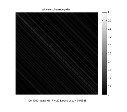
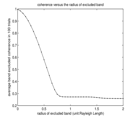
Figure 2: Left: The coherence pattern $[\mu(j,k)]$ of a $100\times 4000$ matrix (5) with $F=20$. Right: A semi-cross section of the coherence band averaged over 100 independent realizations of (4).

Figure 2 shows the coherence pattern from the one-dimensional setting. In two or three dimensions, the coherent pattern is more complicated because the coherence band corresponds to the higher dimensional neighborhood.

More generally, coherent bands can arise in sparse and redundant representation by overcomplete dictionaries. Following Duarte and Baraniuk⁵ we consider the following CS problem

$$\mathbf{b}={\mathbf{\Phi}}\mathbf{y}+{\mathbf{e}}$$ (11)

with a $N\times R$ i.i.d Gaussian matrix ${\mathbf{\Phi}}$ where the signal $\mathbf{y}$ is represented by a redundant dictionary ${\mathbf{\Psi}}$. For example, suppose the sparsifying dictionary is the over-sampled, redundant DFT frame

$$\Psi_{k,j}=\frac{1}{\sqrt{R}}e^{-2\pi i\frac{(k-1)(j-1)}{RF}},\quad k=1,...,R,\quad j=1,...,RF.$$ (12)

where $F$ is the redundancy factor. Writing $\mathbf{y}={\mathbf{\Psi}}\mathbf{x}$ we have the same form (6) with ${\mathbf{A}}={\mathbf{\Phi}}{\mathbf{\Psi}}$. The coherence bands of ${\mathbf{\Psi}}$ and ${\mathbf{A}}$ have the similar structure as shown in Figure 2.

Without extra prior information besides the object sparsity, the CS techniques can not guarantee to recover the objects. The additional prior information we impose here is that the objects are sufficiently separated with respect to the coherence band (see below for details). And we propose modified versions of Orthogonal Matching Pursuit (OMP) for handling highly coherent measurement matrices.

The rest of the paper is organized as follows. In Section 2, we introduce the algorithm, BOMP, to deal with highly coherent measurement matrices and states a performance guarantee for BOMP. In Section 3, we introduce another technique, Local Optimization, to enhance BOMP’s performance and state the performance guarantee for the resulting algorithm, BLOOMP. In Section 4, we present numerical results for the two examples discussed above and compare the existing algorithms with ours. We conclude in Section 5.

2. BAND-EXCLUDED OMP (BOMP)

The first technique that we introduce to take advantage of the prior information of widely separated objects is called Band Exclusion and can be easily embedded in the greedy algorithm, Orthogonal Matching Pursuit (OMP).

Let $\eta>0$. Define the $\eta$-coherence band of the index $k$ as

$$B_{\eta}(k)=\{i\ |\ \mu(i,k)>\eta\},$$ (13)

and the secondary coherence band as

$$B^{(2)}_{\eta}(k) \equiv B_{\eta}(B_{\eta}(k))=\displaystyle\cup_{j\in B_{\eta}(k)}B_{\eta}(j)$$ (14)

Embedding the technique of coherence band exclusion in OMP yields the following algorithm.

Algorithm 1. Band-excluded Orthogonal Matching Pursuit (BOMP)

Input: ${\mathbf{A}},\mathbf{b},\eta>0$

Initialization: $\mathbf{x}^{0}=0,\mathbf{r}^{0}=\mathbf{b}$ and $S^{0}=\emptyset$

Iteration: For $n=1,...,s$

1) $i_{\rm max}=\hbox{arg}\max_{i}|\left\langle\mathbf{r}^{n-1},{\mathbf{a}}_{i}\right\rangle|,i\notin B^{(2)}_{\eta}(S^{n-1})$

2) $S^{n}=S^{n-1}\cup\{i_{\rm max}\}$

3) $\mathbf{x}^{n}=\hbox{arg}\min_{\mathbf{z}}\|{\mathbf{A}}{\mathbf{z}}-\mathbf{b}\|_{2}$ s.t. supp(${\mathbf{z}}$) $\in S^{n}$

4) $\mathbf{r}^{n}=\mathbf{b}-{\mathbf{A}}\mathbf{x}^{n}$

Output: $\mathbf{x}^{s}$.

We have the following performance guarantee for BOMP⁸.

Theorem 1.

Let $\mathbf{x}$ be $s$-sparse. Let $\eta>0$ be fixed. Suppose that

$$B_{\eta}(i)\cap B^{(2)}_{\eta}(j)=\emptyset,\quad\forall i,j\in\hbox{supp}(\mathbf{x})$$ (15)

and that

$$\eta(5s-4)\frac{x_{\text{max}}}{x_{\text{min}}}+\frac{5\|{\mathbf{e}}\|_{2}}{2x_{\text{min}}}<1$$ (16)

where

$$x_{\text{max}}=\max_{k}|x_{k}|,\quad x_{\text{min}}=\min_{k}|x_{k}|.$$

Let $\hat{\mathbf{x}}$ be the BOMP reconstruction. Then $\hbox{supp}(\hat{\mathbf{x}})\subseteq B_{\eta}(\hbox{supp}(\mathbf{x}))$ and moreover every nonzero component of $\hat{\mathbf{x}}$ is in the $\eta$-coherence band of a unique nonzero component of $\mathbf{x}$.

Remark 1.

In the case of the matrix (5), if every two indices in ${\hbox{supp}(\mathbf{x})}$ is more than one RL apart, then $\eta$ is small for sufficiently large $N$, cf. Figure  2.

When the dynamic range ${x_{\text{max}}}/{x_{\text{min}}}=\mathcal{O}(1)$, Theorem 1 guarantees approximate recovery of $\mathcal{O}(\eta^{-1})$ sparsity pattern by BOMP. Since $\eta=\mathcal{O}(N^{-1/2})$ for $N\gg 1$, the sparsity constrain by (16) has the same order of magnitude as the condition for OMP’s performance⁴ in the presence of noise.

The main difference between (16) and the OMP result lies in the role played by the dynamic range $x_{\text{max}}/x_{\text{min}}$ which is absent in the condition for OMP’s performance. Numerical evidence points to the sensitive dependence of BOMP’s performance on dynamic range (Figure 4).

Remark 2.

Condition (15) means that BOMP has a resolution length no worse than 3 $\ell_{R}$ independent of the refinement factor. Numerical experiments show that BOMP can resolve objects separated by close to 1 $\ell_{R}$ when the dynamic range is close to 1.

3. BAND-EXCLUDED, LOCALLY OPTIMIZED OMP (BLOOMP)

We now introduce the second technique, the Local Optimization (LO), to improve the performance of BOMP.

LO is a residual-reduction technique applied to the current estimate $S^{k}$ of the object support. To this end, we minimize the residual ${\|{\mathbf{A}}\hat{\mathbf{x}}-\mathbf{b}\|_{2}}$ by varying one location at a time while all other locations held fixed. In each step we consider $\hat{\mathbf{x}}$ whose support differs from $S^{n}$ by at most one index in the coherence band of $S^{n}$ but whose amplitude is chosen to minimize the residual. The search is local in the sense that during the search in the coherence band of one nonzero component the locations of other nonzero components are fixed. The total number of search is $\mathcal{O}(s^{2}F)$. The amplitudes of the improved estimate is carried out by solving the least squares problem. Because of the local nature of the LO step, the computation is not expensive.

Algorithm 2. Local Optimization (LO)

Input:${\mathbf{A}},\mathbf{b},\eta>0,S^{0}=\{i_{1},\ldots,i_{k}\}$.

Iteration: For $n=1,2,...,k$.

1) $\mathbf{x}^{n}=\hbox{arg}\,\,\min_{{\mathbf{z}}}\|{\mathbf{A}}{\mathbf{z}}-\mathbf{b}\|_{2},\quad\hbox{supp}({\mathbf{z}})=(S^{n-1}\backslash\{i_{n}\})\cup\{j_{n}\},$ $j_{n}\in B_{\eta}(\{i_{n}\})$.

2) $S^{n}=\hbox{supp}(\mathbf{x}^{n})$.

Output: $S^{k}$.

We now give a condition under which LO does not spoil the BOMP reconstruction⁸.

Theorem 2.

Let $\eta>0$ and let $\mathbf{x}$ be a $s$-sparse vector such that (15) holds. Let $S^{0}$ and $S^{k}$ be the input and output, respectively, of the LO algorithm.

If

$$x_{\rm min}>(\varepsilon+2(s-1)\eta)\left({1\over 1-\eta}+\sqrt{{1\over(1-\eta)^{2}}+{1\over 1-\eta^{2}}}\right)$$ (17)

and each element of $S^{0}$ is in the $\eta$-coherence band of a unique nonzero component of $\mathbf{x}$, then each element of $S^{k}$ remains in the $\eta$-coherence band of a unique nonzero component of $\mathbf{x}$.

Embedding LO in BOMP gives rise to the Band-excluded, Locally Optimized Orthogonal Matching Pursuit (BLOOMP).

Algorithm 3. Band-excluded, Locally Optimized Orthogonal Matching Pursuit (BLOOMP)

Input: ${\mathbf{A}},\mathbf{b},\eta>0$

Initialization: $\mathbf{x}^{0}=0,\mathbf{r}^{0}=\mathbf{b}$ and $S^{0}=\emptyset$

Iteration: For $n=1,...,s$

1) $i_{\rm max}=\hbox{arg}\max_{i}|\left\langle\mathbf{r}^{n-1},{\mathbf{a}}_{i}\right\rangle|,i\notin B^{(2)}_{\eta}(S^{n-1})$

2) $S^{n}=\hbox{LO}(S^{n-1}\cup\{i_{\rm max}\})$ where LO is the output of Algorithm 2.

3) $\mathbf{x}^{n}=\hbox{arg}\min_{\mathbf{z}}\|{\mathbf{A}}{\mathbf{z}}-\mathbf{b}\|_{2}$ s.t. supp(${\mathbf{z}}$) $\in S^{n}$

4) $\mathbf{r}^{n}=\mathbf{b}-{\mathbf{A}}\mathbf{x}^{n}$

Output: $\mathbf{x}^{s}$.

Corollary 1.

Let $\hat{\mathbf{x}}$ be the output of BLOOMP. Under the assumptions of Theorems 1 and 2, $\hbox{supp}(\hat{\mathbf{x}})\subseteq B_{\eta}(\hbox{supp}(\mathbf{x}))$ and moreover every nonzero component of $\hat{\mathbf{x}}$ is in the $\eta$-coherence band of a unique nonzero component of $\mathbf{x}$.

Even though we can not improve the performance guarantee for BLOOMP, in practice the LO technique greatly enhances the success probability of recovery with respect to noise stability and dynamic range. Moreover, if Corollary 1 holds, then for all practical purposes we have the residual bound for the BLOOMP reconstruction $\hat{\mathbf{x}}$

$$\|\mathbf{b}-{\mathbf{A}}\hat{\mathbf{x}}\|_{2}\leq c\|{\mathbf{e}}\|_{2},\quad c\sim 1.$$ (18)

4. NUMERICAL RESULTS

We test the algorithms, BOMP and BLOOMP, on the two examples discussed in the Introduction.

For the first example (4)-(6), we use the refinement factor $F=20$. For the objects $\mathbf{x}$, we use 10 randomly phased and located objects, separated by at least 3 $\ell_{R}$. The noise is the i.i.d. Gaussian noise ${\mathbf{e}}\sim N(0,\sigma^{2}I)$.

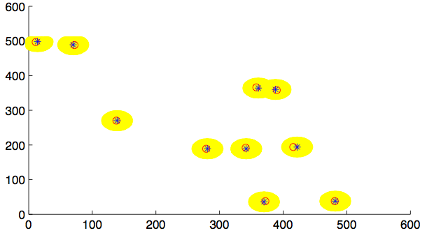
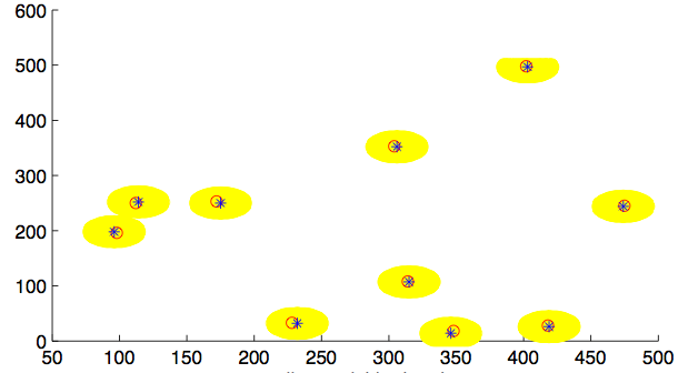
Figure 3: Two instances of BOMP reconstruction: red circles are the exact locations, blue asterisks are recovered locations and the yellow patches are the coherence bands around the objects.

Figure 3 shows two instances of reconstruction by BOMP in two dimensions. The recovered objects (blue asterisks) are close to the true objects (red circles) well within the coherence bands (yellow patches).

For the rest of simulations, we show the percentage of successes in 100 independent trials. A reconstruction is counted as a success if every reconstructed object is within 1 $\ell_{R}$ of the object support. This is equivalent to the criterion that the Bottleneck distance between the true support and the reconstructed support is less than 1 $\ell_{R}$. The result is shown in Figure 4. With 10 objects of dynamic range $5$, BLOOMP requires the least number of measurements, followed by BOMP and then OMP, which does not achieve high success rate even with 100 measurements (left panel). With 100 measurements ($N=100$) and $1\%$ noise, BLOOMP can handle dynamic range up to 120 while BOMP and OMP can handle dynamic range about 5 and 1, respectively.

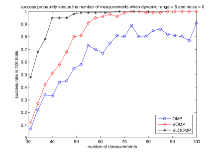
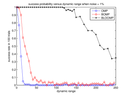
Figure 4: Success rate versus number of measurements (left, dynamic range 5, zero noise) and dynamic range (right, $1\%$ noise) for OMP, BOMP and BLOOMP.

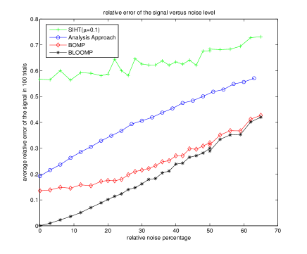
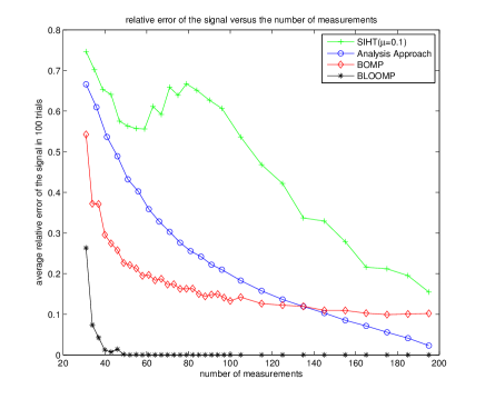
Figure 5: Relative errors versus relative noise (left) and number of measurements (right, zero noise) for dynamic range 10.

For the second example (11)-(12), we test, in addition to our algorithms, the method proposed by Duarte and Baraniuk⁵ and the analysis approach of frame-adapted Basis Pursuit^2,6.

The algorithm, Spectral Iterative Hard Thresholding (SIHT)⁵, assumes the model-based RIP which, in spirit, is equivalent to the assumption of well separated support in the synthesis coefficients and therefore resembles closely to our approach.

While SIHT is a synthesis method like BOMP and BLOOMP, the frame-adapted BP

$$\text{min}\|{\mathbf{\Psi}}^{\star}{\mathbf{z}}\|_{1}\qquad\text{ s.t }\|{\mathbf{\Phi}}{\mathbf{z}}-\mathbf{b}\|_{2}\leq\|{\mathbf{e}}\|_{2},$$ (19)

is the analysis approach⁶. Candès et al.² have established a performance guarantee for (19) provided that the measurement matrix ${\mathbf{\Phi}}$ satisfies the frame-adapted RIP:

$$(1-\delta)\|{\mathbf{\Psi}}{\mathbf{z}}\|_{2}\leq\|{\mathbf{\Phi}}{\mathbf{\Psi}}{\mathbf{z}}\|_{2}\leq(1+\delta)\|{\mathbf{\Psi}}z\|_{2},\quad\|{\mathbf{z}}\|_{0}\leq 2s$$ (20)

for a tight frame ${\mathbf{\Psi}}$ and a sufficiently small $\delta$ and that the analysis coefficients ${\mathbf{\Psi}}^{*}\mathbf{y}$ are sparse or compressible.

Instead of the synthesis coefficients $\mathbf{x}$, however, the quantities of interest are $\mathbf{y}$. Accordingly we measure the performance by the relative error $\|\hat{\mathbf{y}}-\mathbf{y}\|_{2}/\|\mathbf{y}\|_{2}$ averaged over 100 independent trials. In each trial, 10 randomly phased and located objects (i.e. $\mathbf{x}$) of dynamic range 10 and i.i.d. Gaussian ${\mathbf{\Phi}}$ are generated. We set $N=100,R=200,F=20$ for test of noise stability and vary $N$ for test of measurement compression.

As shown in Figure 5, BLOOMP is the best performer in noise stability (left panel) and measurement compression (right panel). BLOOMP requires about 40 measurements to achieve nearly perfect reconstruction while the other methods require more than 200 measurements. Despite the powerful error bound established in [2], the analysis approach (19) needs more than 200 measurements for accurate recovery because the analysis coefficients ${\mathbf{\Psi}}^{*}\mathbf{y}$ are typically not sparse. Here redundancy $F=20$ produces about $2F=40$ highly coherent columns around each synthesis coefficient and hence ${\mathbf{\Psi}}^{*}\mathbf{y}$ has about $400$ significant components. In general, the sparsity of the analysis coefficients is at least $2sF$ where $s$ is the sparsity of the widely separated synthesis coefficients and $F$ is the redundancy. Thus according to the error bound of [2] the performance of the analysis approach (19) would degrade with the redundancy of the dictionary.

To understand the superior performance of BLOOMP in this set-up let us give an error bound using (18) and (20)

$$\|{\mathbf{\Psi}}(\mathbf{x}-\hat{\mathbf{x}})\|_{2}\leq{1\over 1-\delta}\|{\mathbf{A}}(\mathbf{x}-\hat{\mathbf{x}})\|_{2}\leq{1\over 1-\delta}\|\mathbf{b}-{\mathbf{e}}-{\mathbf{A}}\hat{\mathbf{x}}\|_{2}\leq{1+c\over 1-\delta}\|{\mathbf{e}}\|_{2}$$ (21)

where $\hat{\mathbf{x}}$ is the output of BLOOMP. This implies that the reconstruction error of BLOOMP is essentially determined by the external noise, consistent with the left and right panels of Figure 5, and is independent of the dictionary redundancy if Corollary 1 holds. In comparison, the BOMP result appears to approach an asymptote of nonzero ($\sim 10\%$) error. This demonstrates the effect of local optimization technique in reducing error. The advantage of BLOOMP over BOMP, however, disappears in the presence of large external noise (left panel).

5. CONCLUSION

We have proposed algorithms, BOMP and BLOOMP, for sparse recovery with highly coherent, redundant sensing matrices and have established performance guarantee that is redundancy independent. These algorithms have a sparsity constraint and computational cost similar to OMP’s. Our work is inspired by the redundancy-independent performance guarantee recently established for the MUSIC algorithm for array processing.⁷

Our algorithms are based on variants of OMP enhanced by two novel techniques: band exclusion and local optimization. We have extended these techniques to various CS algorithms, including Lasso, and performed systematic tests elsewhere⁸.

Numerical results demonstrate the superiority of BLO-based algorithms for reconstruction of sparse objects separated by above the Rayleigh threshold.

Acknowledgements. The research is partially supported in part by NSF Grant DMS 0908535.

References

- [1] Born, M. and Wolf, E., [Principles of Optics], 7-th edition, Cambridge University Press, 1999.
- [2] Candès, E.J. Eldar, Y.C., Needell, D and Randall, P., “Compressed sensing with coherent and redundant dictionaries,” Appl. Comput. Harmon. Anal. 31 (1), 59–73 (2011)
- [3] Chi, Y., Pezeshki, A., Scharf, L. and Calderbank, R., “Sensitivity to basis mismatch in compressed sensing,” International Conference on Acoustics, Speech, and Signal Processing (ICASSP). Dallas, Texas, Mar. 2010.
- [4] Donoho, D.L., Elad, M. and Temlyakov, V.N., “Stable recovery of sparse overcomplete representations in the presence of noise,” IEEE Trans. Inform. Theory 52, 6-18 (2006).
- [5] Duarte, M.F. and Baraniuk, R.G., “Spectral compressive sensing,” preprint, 2010.
- [6] Elad, M., Milanfar, P. and Rubinstein, R., ” Analysis versus synthesis in signal prior,” Inverse Problems 23, 947-968 (2007).
- [7] Fannjiang, A., ”The MUSIC algorithm for sparse objects: a compressed sensing analysis,” Inverse Problems 27, 035013 (2011).
- [8] Fannjiang, A. and Liao, W., ”Coherence pattern-guided compressive sensing with unresolved grids,” arXiv:1106.5177