Atmospheres of Hot Super-Earths

Abstract

Hot super-Earths likely possess minimal atmospheres established through vapor saturation equilibrium with the ground. We solve the hydrodynamics of these tenuous atmospheres at the surface of Corot-7b, Kepler 10b and 55 Cnc-e, including idealized treatments of magnetic drag and ohmic dissipation. We find that atmospheric pressures remain close to their local saturation values in all cases. Despite the emergence of strongly supersonic winds which carry sublimating mass away from the substellar point, the atmospheres do not extend much beyond the day-night terminators. Ground temperatures, which determine the planetary thermal (infrared) signature, are largely unaffected by exchanges with the atmosphere and thus follow the effective irradiation pattern. Atmospheric temperatures, however, which control cloud condensation and thus albedo properties, can deviate substantially from the irradiation pattern. Magnetic drag and ohmic dissipation can also strongly impact the atmospheric behavior, depending on atmospheric composition and the planetary magnetic field strength. We conclude that hot super-Earths could exhibit interesting signatures in reflection (and possibly in emission) which would trace a combination of their ground, atmospheric and magnetic properties.

1 Introduction

Hot super-Earths are an emerging class of exoplanets. CoRot 7b, Kepler 10b and 55 Cnc-e are currently the only well-characterized, transiting members of this new class (Leger et al. 2009; Batalha et al. 2011; Fischer et al. 2008; Winn et al. 2011; Demory et al. 2011) but observational trends suggest that many more hot super-Earths will be discovered and characterized in the future (e.g., Howard et al. 2011; Borucki et al. 2011).

Structural and evolutionary considerations suggest that hot super-Earths are rocky planets which have lost their original volatile atmospheres, and possibly even some of their rocky material, via atmospheric erosion (Valencia et al. 2010). Indeed, a hot rocky super-Earth will retain a minimal atmosphere that is continuously replenished via vapor saturation equilibrium with the ground (Schaefer & Fegley 2009; Leger et al. 2011) and is thus perpetually subject to erosion. Hot super-Earths are also expected to be tidally-locked to their parent stars. Under these conditions, large temperature and surface pressure differences will exist between the day and the night sides of these planets. By contrast with the majority of known planetary atmospheres, which have a well distributed atmospheric mass around the planet, an unusual circulation regime will thus develop at the surface of hot super-Earths, with powerful winds dynamically redistributing atmospheric mass via exchanges with the ground.

Understanding the atmospheric behavior of hot super-Earths is important for the interpretation of direct observational data and because it informs evolutionary considerations such as atmospheric erosion. In this Letter, we study the unusual hydrodynamics of the atmosphere of hot super-Earths, using a simple model inspired by related work on Io (Ingersoll et al. 1985). In §2, we describe our model hypotheses, equations and method of solution. Our main results are presented in §3. We conclude by discussing some potential implications of our work in §4.

2 Model

2.1 Hypotheses

We consider hot super-Earths that are tidally-locked to their parent stars and thus possess permanent day and night sides. We treat the atmosphere as a continuous fluid that is hydrostatically bound to the planet. The fluid approximation is justified, even if only marginally so in the most tenuous regions described by our solutions, where one runs out of atmosphere near the planetary day-night terminator. For simplicity, we ignore rotation and Coriolis effects in our analysis, so that point symmetry around the substellar point can be assumed. Comparing the rotation timescale ($1/\Omega$) for the three super-Earths of interest with the advection time across a planetary radius ($r/V$) we find Rossby numbers $\sim 2$ for the typical velocities $\sim$ km/s obtained in our solutions. It is thus reasonable to neglect rotation as a first approximation but improved models may need to account for it.

The atmospheric composition that results from vapor saturation equilibrium with the ground on a hot super-Earth is a priori unknown. The analysis of Schaefer & Fegley (2009) for such sublimating atmospheres suggests that monatomic sodium is the dominant constituent on a hot super-Earth with a bulk silicate earth composition, prior to any fractional loss. According to their analysis, this is also the case with the largest overall atmospheric mass (surface pressures). Therefore, without loss of generality, we adopt a pure sodium composition in our models, so as to maximize atmospheric effects in the solutions, and we comment on the consequences of adopting other compositions. Since the atmospheres of interest are tenuous, typically $100$ mbar or much less, we assume that the absorption optical depths in the thermal and the visible are negligibly small ($\ll 1$). Non-radiative considerations, in particular dynamics and exchanges with the ground, will then determine the thermodynamical state of the atmosphere.

We postulate, and verify a posteriori, that latent heat exchanges with the atmosphere have at most a small effect on the surface energy budget, which is dominated by radiative fluxes. We therefore assume that the ground temperature, $T_{s}$, can be obtained by simple radiative balance for the permanent dayside: $T_{s}=(T_{sub}-T_{as})\cos^{1/4}\theta+T_{as}$ for $\theta<85\char 23\relax$, where $\theta$ is the angle away from the substellar point, $T_{sub}$ is the substellar temperature, and $T_{as}$ is the antistellar temperature. For $85\char 23\relax\leq\theta<110\char 23\relax$, we assume that the temperature decreases linearly with $\theta$ to $T_{as}=50$ K, a value which may be reasonable on the basis of geothermal heating of the nightside (Leger et al. 2011), with little consequences on our results. The substellar surface temperature is evaluated simply as $T_{sub}=T_{\star}\sqrt{R_{\star}/D}$, where $T_{\star}$ and $R_{\star}$ are the stellar effective temperature and radius, $D$ is the planet-star orbital separation and a negligible albedo is assumed.

2.2 Equations

Our formalism is directly inspired from that used by Ingersoll et al. (1985) for the study of a frost atmosphere on Io. Indeed, we validated our implementation by reproducing the results for Io first, before moving on to super-Earths. Like Ingersoll et al. (1985), we consider that strong vertical exchanges in the thin, turbulent atmosphere justify the use of vertically-integrated equations for the conservation of atmospheric mass, momentum and energy. Assuming that the velocity and the entropy per unit mass (for a dry adiabat) are constant with height in the atmosphere, the governing equations for the pressure, temperature and velocity at the base of the atmosphere can be written (see Ingersoll et al. 1985 for details):

$$\frac{1}{rg\ \sin\theta}\frac{d}{d\theta}\left(VP\ \sin\theta\right)\ =\ mE,$$ (1)

$$\frac{1}{rg\ \sin\theta}\frac{d}{d\theta}\left[\left(V^{2}\ +\ \beta C_{p}T\right)\ P\ \sin\theta\right]\ =\ \frac{1}{rg\ \tan\theta}\beta C_{p}TP\ +\ \tau,$$ (2)

$$\frac{1}{rg\ \sin\theta}\frac{d}{d\theta}\left[\left(\frac{V^{2}}{2}\ +\ C_{p}T\right)VP\ \sin\theta\right]\ =\ Q,$$ (3)

where $r$ is the planetary radius and $g$ is the planet’s surface gravity. The three unknowns of the atmospheric flow are the velocity, $V$, the pressure, $P$, and the temperature, $T$, at the base of the atmosphere. The thermodynamic parameter $\beta={\cal R/(R}\ +\ C_{p})$, where ${\cal R}=k_{\rm B}/m$ is the gas constant and $C_{p}$ is the specific heat at constant pressure. For sodium, with a mean molecular weight $\mu=23$ and a mass per atom $m=\mu m_{\rm H}$, we adopt the monatomic values $C_{p}=904$ J K^-1 kg^-1 and $\beta=0.286$.

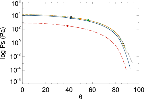
Figure 1: Atmospheric pressure (in Pascal) as a function of the angular distance from the substellar point. Blue solid, red long-dashed and black dotted lines show the results for a sodium atmosphere on 55 Cnc e, Corot-7b, 55 and Kepler-10b, respectively. Solutions with magnetic effects for Kepler-10b are also shown with yellow dash-dotted ($T_{drag}=10^{4}$ s) and green short-dashed ($T_{drag}=5\times 10^{3}$ s) lines. Dots represent the sonic point location.

$E$, $\tau$, and $Q$ are the rates per unit area of molecules, momentum and energy transferred to the atmosphere by exchange with the ground. These fluxes, which are mediated by a boundary layer of negligible vertical extent at the base of the atmosphere, are governed by sublimation/condensation processes, flow advection, and turbulent exchanges by eddies. Our implementation of these surface-atmosphere boundary layer exchanges follows closely that adopted by Ingersoll et al. (1985). The net flux of sublimating/condensating molecules is proportional to the difference between the vapor pressure $P_{v}$ of the surface and the atmospheric pressure $P$, so that $E\ =\ {(P_{s}\ -\ P)}/({v_{s}\sqrt{2\pi}})$, where $v_{s}=(kT_{s}/m)^{1/2}$ is the molecular thermal speed at the surface. We approximate the vapor pressure curve of sodium by fitting the sodium curve for the bulk silicate atmosphere model shown in Figure 1 of Schaefer & Fegley (2009) with the formula $P_{s}(T_{s})=A\exp(-B/T_{s})$. We adopt $A=10^{9.6}$ Pa and $B=38,000$ K.

The fluxes $Q$ and $\tau$ depend linearly on the quantities being transported, with the same transfer coefficients $w_{s}$ and $w_{a}$. Energy gains from the surface are proportional to the enthalpy per unit of mass at the surface, $C_{p}T_{s}$, while losses scale as the sum of the kinetic energy and enthalpy per unit mass, $(V^{2}/2\ +\ C_{p}T)$. For momentum, gains from the surface are zero, while losses are proportional to $V$. This leads to the formulation

$$\tau\ =\ -\rho_{s}w_{a}V,$$ (4)

$$Q\ =\ \rho_{s}w_{s}C_{p}T_{s}\ -\ \rho_{s}w_{a}(V^{2}/2\ +\ C_{p}T),$$ (5)

where $\rho_{s}=mP_{s}/(k_{b}T_{s})$ is the density in the boundary layer. Two different contributions are included in the definition of the transfer coefficients $w_{a}$ and $w_{d}$. First, the contribution from the mean flow normal to the surface is proportional to $E$ and is represented by the velocity $V_{e}=mE/\rho_{s}$. Second, the contribution from turbulent eddies is obtained from turbulent boundary layer results in the case $E=0$. We adopt the same expressions for the transfer coefficients $w_{a}$ and $w_{d}$ as Ingersoll et al. (1985). Finally, where needed, we use Sutherland’s ideal gas formula to evaluate the dynamic viscosity of the atmospheric gas: $\eta\ =\ \eta_{0}({T_{s}}/{T_{0}})^{3/2}({T_{0}+C})/({T_{s}+C})$, with $\eta_{0}=1.8\times 10^{-5}$ kg m^-1 s^-1, $T_{0}=291$ K and $C=120$ K. We have verified that our results do not strongly depend on details of the viscosity law adopted.

In sufficiently ionized regions, magnetic drag and ohmic dissipation can influence atmospheric flows on hot super-Earths, if these planets possess strong enough magnetic fields (Gaidos et al. 2010; Tachinami et al. 2011; Driscoll & Olson 2011). Here, we build on the recent understanding gained in the context of hot giant exoplanet atmospheres (Batygin & Stevenson 2010; Perna et al. 2010a,b; Menou 2011). Assuming induced electric currents that are confined to the thin atmosphere of hot super-Earths, magnetic drag and ohmic dissipation may be included in the simplest possible way as additional, vertically-integrated contributions to the fluxes of momentum and energy received by the atmosphere, through linear terms proportional to the inverse of a representative magnetic drag time, $T_{drag}$. Therefore, in models including magnetic effects, we add contributions to $\tau$ and $Q$ which act to brake the winds and heat up the atmosphere according to:

$$\tau_{\rm mag}\ =\ -\frac{PV}{gT_{drag}},~{}~{}~{}Q_{\rm mag}\ =+\frac{PV^{2}}{gT_{drag}}.$$ (6)

Adopting a magnetic field strength $B=1$ G, detailed estimates of the resistivity ($\eta$) based on the formalism described in Menou (2011) yield drag times $T_{drag}~{}\propto\eta/B^{2}$ that vary greatly over the planet for a sodium atmosphere. Drag times can be much shorter than a typical advection time, $r/V$, in the vicinity of the hot substellar point, but they can become negligibly large in poorly-ionized regions where $T\mathrel{\hbox to0.0pt{\lower 4.0pt\hbox{\hskip 1.0pt$\sim$}\hss}\raise 1.0pt\hbox{$<$}}1000$ K. Changing the assumed composition to a less easily ionized atom, e.g. from Na to Mg (another possibly abundant constituent; Schaefer & Fegley 2009), can also lead to dramatically reduced magnetic effects. Therefore, rather than exploring magnetic effects in detail here, we illustrate their consequences below by presenting two idealized models for Kepler 10-b with spatially uniform values of $T_{drag}=10^{4}$ and $5\times 10^{3}$ s, which have been chosen to match the typical advection time in our solutions with velocities $\sim$ km/s.

2.3 Method of Solution

We solve our set of differential and auxiliary equations for the unknowns $P,\ T,\ V$ with a relaxation method (specifically, the algorithm described in Hameury et al. 1998). Special care must be taken when integrating these equations because the solution goes through a sonic point at an unspecified angle, $\theta_{s}$. To find $\theta_{s}$, we define $\theta$ as a fourth variable on a numerical domain describing the subsonic region only and we apply physically sensible boundary conditions on this domain.

At the substellar point, $V(\theta=0)=0$ is imposed for symmetry and $T(\theta=0)=T_{sub}$. The transonic solution must have a well-behaved value of $dV/d\theta$ at the sonic point, which provides the two additional boundary conditions needed on the subsonic domain. Noting that the following first-order differential equation is satisfied by the velocity,

$$CpP\left(T-\frac{V^{2}}{{\cal R}}\right)\frac{dV}{d\theta}=\left(\frac{1}{\beta}-\frac{1}{2}\right)mgrV^{2}E-\frac{rgV\tau}{\beta}+rgQ-\frac{C_{p}TPV}{\tan\theta},$$ (7)

requiring a smooth sonic transition leads to the two boundary conditions at $\theta=\theta_{s}$:

$$V=\sqrt{{\cal R}T},\ \ \ P=gr\tan\theta\times\frac{{\cal R}}{C_{p}}\left(\frac{Q}{V^{3}}-\frac{\tau}{\beta V^{2}}+\left(\frac{1}{\beta}-\frac{1}{2}\right)\frac{mE}{V}\right).$$

Our initial guesses for the relaxation method are based on the analytical solutions of Ingersoll (1989), adapted to our super-Earth problem. Once $\theta_{s}$ and the solution on the subsonic domain are known, using a small extrapolation across the sonic point, the integration can proceed in the supersonic domain using a simple Euler method. The integration is stopped when the pressure is so low that the fluid approximation ceases to be valid.

3 Results

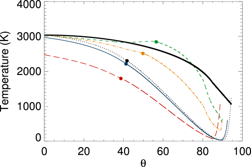
Figure 2: Temperature (in K) at the base of the atmosphere as a function of the angular distance from the substellar point. Same notation as in Fig. 1. A black thick solid line also traces the surface temperature profile adopted in the Kepler 10b models.

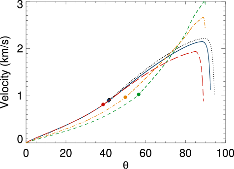
Figure 3: Velocity (in km/s) at the base of the atmosphere as a function of the angular distance from the substellar point. Same notation as in Fig. 1.

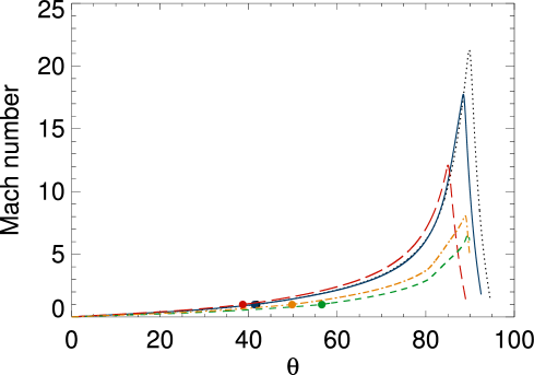
Figure 4: Mach number of the atmospheric flow as a function of the angle from the substellar point. Same notation as in Fig. 1.

We solve the hydrodynamics of sodium atmospheres at the surface of CoRot-7b, Kepler 10b and 55 Cnc-e (see Table 1 for the specific parameters adopted). Figures 1-4 show the pressure, temperature, velocity and Mach number obtained for the base of the atmosphere, as a function of the angular distance from the substellar point. In each figure, large dots indicate the location of the sonic points. Solutions are shown as red long-dashed lines for CoRot-7b, black dotted lines for Kepler 10b and blue solid lines for 55 Cnc-e. In addition, two solutions illustrating magnetic effects for Kepler 10-b are shown as a yellow dash-dotted line ($T_{drag}=10^{4}$ s) and a green short-dashed line ($T_{drag}=5\times 10^{3}$ s). Finally, a thick black solid line in Figure 2 shows the ground temperature in the Kepler 10-b model, for comparison with the atmospheric temperatures.

Ignoring magnetic effects, our atmospheric solutions for the three hot super-Earths share many similarities. CoRot 7-b is essentially a cooler, more tenuous version of Kepler 10b and 55 Cnc-e. This similarity stems from the strong control that vapor saturation equilibrium exerts on the atmospheric flow, via the exponential dependence of pressure on surface temperature, with a comparatively small influence for other model parameters such as planetary radius or surface gravity.

In these atmospheric flows, winds are accelerated by conversion of thermal and gravitational potential energy into kinetic energy. Supersonic speeds are reached at $\theta_{s}\sim 40$ deg. Atmospheric pressures remain close to the local saturation values, within tens of % or so, over most of the flow, with stronger deviations in the end region at $\theta\mathrel{\hbox to0.0pt{\lower 4.0pt\hbox{\hskip 1.0pt$\sim$}\hss}\raise 1.0pt\hbox{$>$}}80$ deg. Distinct regions of atmospheric sublimation ($E>0$) and condensation ($E<0$) roughly correspond to the subsonic and the supersonic regions of the flow, respectively. Beyond $\theta\sim 85$-$90$ deg, where the atmosphere becomes very tenuous, viscous drag becomes very strong and the flow quickly transitions into a regime where kinetic energy is returned into thermal and gravitational energy. Large Mach numbers are achieved before the atmospheric flow effectively comes to a halt. These flow properties are generally consistent with the ones described by Ingersoll et al. (1985) for a sulfur dioxyde frost atmosphere on Io, despite the vastly different thermodynamic regime realized on hot super-Earths. Therefore, we expect these results to hold rather generally for hot super-Earths, including for different atmospheric compositions, even if a reduced angular extent of the flow (limited by strong viscous drag) can be expected for less massive atmospheres.

Magnetic effects complicate this picture significantly. Magnetic drag slows down the winds in the subsonic region, as expected, but larger wind speeds are ultimately reached in the supersonic region. This delayed acceleration can be understood as resulting from the additional thermal and gravitational energy made available to the flow by significant ohmic heating, especially around and beyond the sonic point (compare the temperature profiles of models with and without magnetic effects in Fig. 2). The atmospheric solutions with uniform values of $T_{drag}=10^{4}$ and $5\times 10^{3}$ s for Kepler-10b differ significantly from each other and the unmagnetized case, showing that magnetic effects can have a strong impact on the flow. One should remember that our treatment of these effects remains greatly idealized: magnetic drag may preferentially act on the zonal component of the flow for a dipolar planetary field and the magnitude of this drag (and ohmic dissipation) will vary exponentially with atmospheric temperature (e.g., Menou 2011). The large range of temperatures realized on hot super-Earths suggests a strongly magnetic atmospheric flow near the substellar point and a largely unmagnetized flow far from it (where $T\mathrel{\hbox to0.0pt{\lower 4.0pt\hbox{\hskip 1.0pt$\sim$}\hss}\raise 1.0pt\hbox{$<$}}1000$ K). These important considerations are not addressed by our models.

Our solutions justify a posteriori the use of a fixed surface temperature profile, controlled by radiative fluxes. The evaporation rate peaks at a few $10^{24}$ m^-2 s^-1 at the substellar point, drops to zero near the sonic point and reaches minimal values of minus a few $10^{23}$ m^-2 s^-1 around $\theta\sim 60$ deg. Given a latent heat of sublimation ${\cal{L}_{\rm sub}}\sim 10^{5}$-$10^{6}$ J kg^-1 for atmospheric compositions of interest (e.g., Valencia et al. 2010), we estimate deviations from the radiative temperature profile due to latent heat effects which are at most $\sim$ a few % at the substellar point. They can be neglected in view of other sources of uncertainties in the model.

4 Discussion and Conclusion

According to our solutions, the range of atmospheric temperatures and pressures realized on the day-side of a hot super-Earth is vast. Rather than a pure composition like sodium, it is likely that such an atmosphere would also include minor constituents which are subject to condensation into clouds, as discussed by Schaefer & Fegley (2009). The diverse range of thermodynamic conditions in the atmosphere across the dayside opens the possibility for the formation of many different classes of clouds. If some of these clouds are thick and reflective enough, they could dominate the planetary albedo properties of a hot super-Earth, given surface albedos of only $\sim 0.1$ (Leger et al. 2011). This may lead to interesting signatures in the reflected light from a hot super-Earth, if for instance strong albedo variations occur across the planetary dayside. A large enough albedo from clouds ($\mathrel{\hbox to0.0pt{\lower 4.0pt\hbox{\hskip 1.0pt$\sim$}\hss}\raise 1.0pt\hbox{$>$}}0.1$) would also generate variations in the surface irradiation pattern, which would imprint an additional signature in the dayside thermal emission of the planet. Excitingly, the measurable optical phase curve of Kepler 10b could eventually reveal such signatures (Batalha et al. 2011).

Our results show that, even for a relatively massive sodium atmosphere, the powerful winds which carry sublimating mass away from the substellar point on a hot super-Earth are unable to establish a significant atmosphere beyond the planetary day-night terminator. This conclusion impacts atmospheric erosion scenarios. Traditional assumptions of spherical symmetry and of an atmosphere at rest are poorly justified for hot super-Earths. While magnetized wind scenarios favor atmospheric loss from the polar regions (e.g., Adams 2011; Trammel et al. 2011), where there can be little atmosphere according to our models, it can also be the case that atmospheric temperatures in the polar regions are low enough that magnetic coupling can be neglected. Furthermore, at surface pressures $\mathrel{\hbox to0.0pt{\lower 4.0pt\hbox{\hskip 1.0pt$\sim$}\hss}\raise 1.0pt\hbox{$<$}}10^{-2}$-$10^{-4}$ Pa, which are reached near the terminator in our solutions, the most tenuous part of the atmosphere may become transparent to UV irradiation (Valencia et al. 2010), which would presumably stall erosion.

We conclude by noting that the sublimation/condensation rates obtained in our solutions suggest the possibility of substantial planetary resurfacing by atmospheric transport. The global atmospheric circulation carries mass from the substellar region to a region centered around $\theta\sim 50$-$70$ deg, where net condensation occurs. Over Gyr timescales, this process could impact the atmospheric composition by preferentially transporting some (sublimating) constituents relative to others and, ultimately, coupling the availability of volatiles at the substellar point to internal geodynamic redistribution processes. In principle, strong resurfacing may also influence the tidal response of the rocky planet by gradually modifying its gravitational moments, if condensation occurs beyond the angular extent of the dayside magma ocean (e.g., Leger et al. 2011). Detailed calculations will be needed to evaluate the magnitude of these effects.

Parameter	Kepler-10b	Corot-7b	55 Cnc e
Stellar effective temperature, $T_{\star}$ (K)	5630	5250	5370
Stellar radius, $R_{\star}$ (m)	$7.3\times 10^{8}$	$5.7\times 10^{8}$	$8.0\times 10^{8}$
Orbital distance, D (m)	$2.5\times 10^{9}$	$2.6\times 10^{9}$	$2.3\times 10^{9}$
Planetary radius, r (m)	$9.0\times 10^{6}$	$10.1\times 10^{6}$	$12.8\times 10^{6}$
Planetary surface gravity, g (m s-2)	22.2	27.1	19.6
Planetary substellar temperature, $T_{sub}$ (K)	3040	2470	2970

Table 1: Parameters for Hot Super-Earth Models.

References

- (1) Adams, F. C. 2011, ApJ 730, 27
- (2)
- (3) Batalha, N. M. et al. 2011, ApJ 729, 27
- (4)
- (5) Batygin, K. & Stevenson, D. J. 2010, 714, L238
- (6)
- (7) Borucki, W. J. et al. 2011, ApJ 736, 19
- (8)
- (9) Demory, B.-O. et al. 2011, A&A submitted, arXiv:1105.0415
- (10)
- (11) Driscoll, P. & Olson, P. 2011, Icarus 213, 12
- (12)
- (13) Fischer, D. A. et al. 2008, ApJ 675, 790
- (14)
- (15) Gaidos, E., Conrad, C. P., Manga, M. & Hernlund, J. 2010, ApJ 718, 596
- (16)
- (17) Hameury, J.-M. et al. 1998, MNRAS 298, 1048
- (18)
- (19) Ingersoll, A. P. 1989, Icarus, 81, 298 313
- (20)
- (21) Ingersoll, A. P., Summers, M. E. & Schlipf S. G. 1985, Icarus, 64, 375 390
- (22)
- (23) Leger, A. et al. 2009, A&A 506, 287
- (24)
- (25) Leger, A. et al. 2011, Icarus 213, 11
- (26)
- (27) Menou K. 2011, ApJ submitted, arXiv:1108.3592
- (28)
- (29) Perna, R., Menou, K. & Rauscher, E., 2010a, ApJ 719, 1421
- (30)
- (31) Perna, R., Menou, K. & Rauscher, E., 2010b, ApJ 724, 313
- (32)
- (33) Schaefer L. & Fegley J. B. 2009 ApJ 703, L113
- (34)
- (35) Showman, A. P. & Polvani, L. M. 2011, ApJ 738, 71
- (36)
- (37) Trammel, G. B., Arras, P. & Li, Z.-Y. 2011, ApJ 728, 152
- (38)
- (39) Tachinami, C., Senshu, H. & Ida, S. 2011, ApJ 726, 70
- (40)
- (41) Valencia, D., Ikoma, M., Guillot, T. & Nettelmann, N. 2010 A&A 516, 20
- (42)
- (43) Winn J. N. et al. 2011, arXiv:1104.5230
- (44)