On the Eigenvalue Density of the non-Hermitian Wilson Dirac Operator

Abstract

We find the lattice spacing dependence of the eigenvalue density of the non-Hermitian Wilson Dirac operator in the $\epsilon$-domain. The starting point is the joint probability density of the corresponding random matrix theory. In addition to the density of the complex eigenvalues we also obtain the density of the real eigenvalues separately for positive and negative chiralities as well as an explicit analytical expression for the number of additional real modes.

Introduction.

In the past two decades, there has been an increasing interest in non-Hermitian random matrix theory (RMT) RMT1 . To name a few applications, quantum chaos in open systems SSS , dissipative systems DIS and QCD at finite chemical potential ST . Some features of the model we are considering also occur in the condensed matter system analyzed in Ref. RL .

The connection between the infrared limit of QCD and RMT has been well understood in the continuum limit since the early 90’s ShuVer93 . It is based on the universality of chiral RMT in the microscopic limit (or $\epsilon$ domain) ADMN97 with chiral RMT described by the same chiral Lagrangian as QCD. The main advantage of RMT is the availability of powerful methods to derive analytical results, and recently this approach was applied to QCD at finite lattice spacing osborn ; DSV10 ; ADSV10b ; SplVer11 . It was shown that the $\epsilon$ limit of the chiral Lagrangian for the Wilson Dirac operator $D_{\rm W}$ ShaSin98 ; BRS04 can be obtained from an equivalent RMT. Discretization effects of the spectrum of $D_{\rm W}$ have been studied directly by means of chiral Lagrangians Sha06 ; necco ; DSV10 ; ADSV10b ; SplVer11 , but using RMT methods will enable us to obtain results that were not accessible previously.

The aim of this paper is to obtain analytical results for the eigenvalue density of $D_{\rm W}$ for the RMT model proposed in Ref. DSV10 . We consider the quenched case.

RMT.

We consider the random matrix theory DSV10 ,

$$D_{\rm W} = \left(\begin{array}[]{cc}aA&W\\ -W^{\dagger}&aB\end{array}\right)$$ (3)

distributed by

$$P(D_{\rm W})\propto\exp\left[-\frac{n}{2}(\textrm{tr}A^{2}+\textrm{tr}B^{2})-n\textrm{tr}WW^{\dagger}\right].$$ (4)

The matrices $A$ and $B$ are Hermitian $n\times n$ and $(n+\nu)\times(n+\nu)$ matrices, respectively, and the entries of $W$ are complex and independent. In the microscopic limit, with $n\to\infty$ at fixed rescaled eigenvalues $\widehat{z}=2nz$ and lattice spacing $\widehat{a}^{2}=na^{2}/2$, the spectral properties of this RMT become universal and agree with Wilson chiral perturbation theory in the same limit (with $n$ identified as the volume of space-time) apart from the squared trace terms BRS04 ; Sha06 . The finite integer $|\nu|\leq n$ is the index of the Dirac operator and is kept fixed.

The matrix $D_{\rm W}$ is $\gamma_{5}=\textrm{diag}(\leavevmode\hbox{\small 1\kern-3.8pt\normalsize 1}_{n},-\leavevmode\hbox{\small 1\kern-3.8pt\normalsize 1}_{n+\nu})$-Hermitian, i.e. $D_{\rm W}^{\dagger}=\gamma_{5}D_{\rm W}\gamma_{5}$. Therefore its eigenvalues are either real or come in complex conjugate pairs. The $\nu$ generic zero modes at $a=0$ become the generic real modes of $D_{\rm W}$ at finite lattice spacing. Furthermore, $D_{\rm W}$ may have $2n-2l$ additional real eigenvalues which appear when a pair of complex eigenvalues collides with the real axis.

In Refs. DSV10 ; ADSV10b ; SplVer11 ; AkeNag11 the technically simpler case of the Hermitian Wilson Dirac operator $D_{5}=\gamma_{5}D_{\rm W}$ was studied. Although spectra of $D_{5}$ have been studied in the lattice literature Luscher , only the eigenvalues of $D_{\rm W}$ are directly related to chiral symmetry breaking which is our main motivation to study its spectral properties.

The joint probability distribution (jpd).

To preserve the $\gamma_{5}$-Hermiticity of $D_{\rm W}$ we can only quasi-diagonalize $D_{\rm W}$ by a non-compact unitary matrix $U\in\textrm{U}(n,n+\nu)$,

$$D_{\rm W}=UXU^{-1}\ \textrm{and}\ X=\left(\begin{array}[]{cccc}x_{1}&0&0&0\\ 0&x_{2}&y_{2}&0\\ 0&-y_{2}&x_{2}&0\\ 0&0&0&x_{3}\end{array}\right).$$ (9)

In contrast to the diagonalization of a Hermitian matrix such as $D_{5}$, the matrix $X$ may only be quasi-diagonal where $x_{1}$, $x_{2}$, $y_{2}$ and $x_{3}$ are diagonal matrices of dimension $n-l$, $l$, $l$ and $n-l+\nu$ with $0\leq l\leq n$ the number of complex conjugate pairs. The complex eigenvalues are given by $(z,z^{*})=(x_{2}+\imath y_{2},x_{2}-\imath y_{2})$. The ensemble $D_{\rm W}$ decomposes into $n+1$ disjoint sets of quasi-diagonal matrices (9) with a fixed number of real eigenvalues. The joint probability density of the $2n+\nu$ eigenvalues $Z=(z_{1{\rm r}},\ldots,z_{n{\rm r}},z_{1{\rm l}},\ldots,z_{n+\nu,{\rm l}})\in\mathbb{C}^{2n+\nu}$ can be obtained by integrating over $U$. This calculation will be discussed in detail elsewhere. We only give the result for $\nu\geq 0$ which is not a restriction because of the symmetry $\nu\rightarrow-\nu$. The jpd is given by

$$p(Z)\propto\Delta_{2n+\nu}(Z)\det\left[\begin{array}[]{c}\left\{g_{2}(z_{a{\rm r}},z_{b{\rm l}})\right\}\underset{1\leq b\leq n+\nu}{\underset{1\leq a\leq n}{\ }}\\ \left\{z_{b{\rm l}}^{a-1}g_{1}(z_{b{\rm l}})\right\}\underset{1\leq b\leq n+\nu}{\underset{1\leq a\leq\nu}{\ }}\end{array}\right],$$ (12)

$$g_{1}(z)=\sqrt{\frac{n}{2\pi a^{2}}}\exp\left[-\frac{n}{2a^{2}}x^{2}\right]\delta(y),$$ (13)

$$g_{2}(z_{1},z_{2})=\sqrt{\frac{n^{3}}{4\pi a^{2}(1+a^{2})}}\frac{z_{1}^{*}-z_{2}^{*}}{|z_{1}-z_{2}|}$$

$$\times \left[\exp\left[-\frac{n(x_{1}+x_{2})^{2}}{4a^{2}}-\frac{n(y_{1}-y_{2})^{2}}{4}\right]\delta^{(2)}(z_{1}-z_{2}^{*})\right.$$

$$+ \left.\frac{1}{2}\exp\left[-\frac{n}{4a^{2}}(x_{1}+x_{2})^{2}+\frac{n}{4}(x_{1}-x_{2})^{2}\right]\right.$$

$$\times \left.{\rm erfc}\left[\frac{\sqrt{n(1+a^{2})}}{2a}|x_{1}-x_{2}|\right]\delta(y_{1})\delta(y_{2})\right],$$

$$\equiv g_{2\,{\rm c}}(z_{1})\delta^{(2)}(z_{1}-z_{2}^{*})+g_{2\,{\rm r}}(x_{1},x_{2})\delta(y_{1})\delta(y_{2}),$$

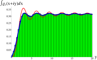
Figure 1: The projection of $\rho_{\rm c}$ onto the imaginary axis for $\nu=1$ and $\widehat{a}=1/\sqrt{8}$. The Monte Carlo simulation (histogram, bin size=0.4) contains 200000 matrices with $n=50$. This simulation nicely confirms our analytical result (blue curve) and shows the deviations from the $\widehat{a}=0$ result (red curve).

where ${\rm erfc}$ is the complementary error function and $\delta^{(2)}(x+\imath y)=\delta(x)\delta(y)$. Due to $\gamma_{5}$ the permutation group $\mathfrak{S}(2n+\nu)$ is broken to $\mathfrak{S}(n)\times\mathfrak{S}(n+\nu)$ which reflects itself in the product of the Vandermonde determinant $\Delta_{2n+\nu}(Z)$ and the other determinant in Eq. (13). The expansion of the delta functions yields the jpd for each of the $n+1$ subsets with a fixed number of complex eigenvalue pairs. The two-point distribution $g_{2}$ splits into one term for the real eigenvalues $g_{2{\rm r}}$ and one for the complex conjugated pairs $g_{2{\rm c}}$ as it is also known for the real Ginibre ensemble and its chiral counterpart Gin .

The eigenvalue densities

for the real and complex eigenvalues can be obtained by integrating over all eigenvalues except one. The spectral density can be decomposed into the density of real modes, $\rho_{\rm r}$ for positive chirality ($\langle\psi|\gamma_{5}|\psi\rangle>0$), $\rho_{\rm l}$ for negative chirality ($\langle\psi|\gamma_{5}|\psi\rangle<0$), and the density of complex pairs, $\rho_{\rm c}$,

$$\int p(Z)\prod_{z_{j}\neq z_{1{\rm r}}}d[z_{j}] = \rho_{\rm r}(x_{1{\rm r}})\delta(y_{1{\rm r}})+\frac{\rho_{\rm c}(z_{1{\rm r}})}{2},$$ (14)

$$\int p(Z)\prod_{z_{j}\neq z_{1{\rm l}}}d[z_{j}] = \rho_{\rm l}(x_{1{\rm l}})\delta(y_{1{\rm l}})+\frac{\rho_{\rm c}(z_{1{\rm l}})}{2}.$$ (15)

Note that the chirality reflects the conventions of the RMT. By expanding the first row of the determinant in Eq. (13) and re-expressing the additional factors from $\Delta_{2n+\nu}(Z)$ as $N_{\rm f}=2$ partition functions we obtain

$$\rho_{\rm c}(z) = g_{2{\rm c}}(z)(z-z^{*})Z_{N_{\rm f}=2}^{\nu}(z,z^{*};a),$$ (16)

$$\rho_{\rm r}(x) = \int_{\mathbb{R}}g_{2{\rm r}}(x,x^{\prime})(x-x^{\prime})Z_{N_{\rm f}=2}^{\nu}(x,x^{\prime};a)dx^{\prime}.$$ (17)

A similar factorized structure was found in Ref. Splittorff:2003cu .

Expanding the first column of the determinant and integrating over all eigenvalues except $z_{1l}$, we find the same expression for $\rho_{\rm c}$ and the density $\rho_{\rm l}$ of the real modes originating from $g_{2}$ (using Eq. (6)). However, there is an additional contribution to $\rho_{\rm r}$ due to the last $\nu$ rows which gives the distribution of chirality over the real eigenvalues

$$\rho_{\chi}=\rho_{\rm l}-\rho_{\rm r}.$$ (18)

Additional rows of some of the determinants have to be expanded to express them into known partition functions. We have checked for $\nu=1$ and $\nu=2$ that the result agrees with previously derived expressions DSV10 ; SplVer11 .

In the microscopic limit, the partition functions in Eqs. (16) and (17) can be expressed in terms of integrals over $\textrm{U}(2)$. They can be simplified using the eigenvalues of the $\textrm{U}(2)$-matrices as integration variables resulting in

$$\rho_{\rm c}\left(\frac{z}{2n}\right) = \frac{e^{-x^{2}/8\widehat{a}^{2}}|y|}{(2\pi)^{5/2}2\widehat{a}}\int_{[0,2\pi]^{2}}e^{x(\cos\varphi_{1}+\cos\varphi_{2})-4\widehat{a}^{2}(\cos^{2}\varphi_{1}+\cos^{2}\varphi_{2})}{\rm sinc}[y(\cos\varphi_{1}-\cos\varphi_{2})]\cos\nu(\varphi_{1}+\varphi_{2})D\varphi_{k},$$ (19)

$$\rho_{\rm r}\left(\frac{x}{2n}\right) = \frac{1}{16\pi^{2}}\int_{[0,2\pi]^{2}}\frac{\exp[\Delta_{1}^{2}-\Delta_{2}^{2}]{\rm erf}\left[\Delta_{1},\sqrt{2}\Delta_{1}\right]-\exp[\Delta_{2}^{2}-\Delta_{1}^{2}]{\rm erf}\left[\Delta_{2},\sqrt{2}\Delta_{2}\right]}{\cos\varphi_{1}-\cos\varphi_{2}}\cos\nu(\varphi_{1}+\varphi_{2})D\varphi_{k},$$ (20)

$$\rho_{\chi}\left(\frac{x}{2n}\right) = \frac{(-1)^{\nu}}{16\pi\widehat{a}^{2}}\int_{\mathbb{R}^{2}}\frac{e^{-((s_{1}-x)^{2}+(s_{2}+ix)^{2})/16\widehat{a}^{2}}}{s_{1}-\imath s_{2}}s_{1}^{\nu}\left[s_{1}K_{\nu+1}(s_{1})I_{\nu}(\imath s_{2})+\imath s_{2}K_{\nu}(s_{1})I_{\nu+1}(\imath s_{2})\right]\frac{\delta^{(\nu-1)}(s_{1})}{(\nu-1)!}ds_{1}ds_{2}.$$ (21)

The functions ${\rm sinc}$, ${\rm erf}$, $I_{l}$, $K_{l}$ and $\delta^{(l)}$ are the sinus cardinalis, the generalized incomplete error function

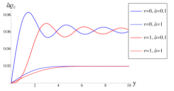
Figure 2: Along the imaginary axis the difference of $\rho_{\rm c}$ for different $\nu$ is much clearer at small $\widehat{a}$ (solid curves) than at large $\widehat{a}$ (dashed curves) where they are almost the same.

(${\rm erf}(b,c)={\rm erf}(c)-{\rm erf}(b)$), modified Bessel function of the first and second kind and the $l$-th derivative of the Dirac delta function, respectively. The integration measure is induced by the invariant $\textrm{U}(2)$ measure, $D\varphi_{k}=$ $\sin^{2}((\varphi_{1}-\varphi_{2})/2)d\varphi_{1}d\varphi_{2}$ and $\Delta_{j}=2\widehat{a}\left(\cos\varphi_{j}-{x}/{8\widehat{a}^{2}}\right)$. Because of the $\delta$-function only the algebraic singular part of the $K_{\nu}$ contributes to $\rho_{\chi}$ (which was already obtained in Refs. DSV10 ; SplVer11 ). The distribution $\rho_{\chi}$ vanishes for $\nu=0$ and can be obtained from the generating function for the eigenvalue density of $\gamma_{5}(D_{W}+m)$. DSV10 Comparisons of the analytical results with simulations of the random matrix model (3) are shown in Figs. 1 and 4. The normalizations are chosen such that the integral over $\rho_{\chi}$ is equal to $\nu$. The other constants are already fixed by this choice.

For small increasing $\widehat{a}$ the complex eigenvalues move parallel to the real axis according to a Gaussian distribution with a width of $2\widehat{a}$ (See Fig. 3). Therefore the density of the projection of these eigenvalues on the imaginary axis is very close to the $\widehat{a}=0$ result. For large $\widehat{a}$ the distribution of the real parts of the complex eigenvalues develops a box-like shape from $-8\widehat{a}^{2}$ to $8\widehat{a}^{2}$ which can be derived from a saddle point approximation of Eq. (19) (See Fig. 3) and the oscillations disappear (See Fig. 2). Along the imaginary axis $\rho_{\rm c}(\widehat{a}\gg 1)$ becomes $\widehat{a}^{-2}{\rm erf}(y/4\widehat{a})$.

Near the real axis $\rho_{\rm c}$ behaves as $y^{\nu+1}$ for small $\widehat{a}$ but is linear in $y$ for $\widehat{a}$ large enough (See Fig. 2). In the continuum limit it peaks around the imaginary axis and eventually gets the form of the continuum microscopic eigenvalue density.

Real modes.

For a Wilson Dirac operator with index $\nu$ there are at least $\nu$ real modes. The additional real modes result when complex conjugate eigenvalue pairs enter the real axis. The average number of these modes follows from the integral

$$N_{\rm add}=2\int_{\mathbb{R}}\rho_{\rm r}\left(\frac{x}{2n}\right)dx\hskip 85.35826pt$$ (22)

$$=\int_{[0,2\pi]^{2}}\frac{1-e^{-2\widehat{a}^{2}(\cos\varphi_{1}-\cos\varphi_{2})^{2}}}{8\pi^{2}\sin^{2}((\varphi_{1}+\varphi_{2})/2)}\cos\nu(\varphi_{1}+\varphi_{2})d\varphi_{1}d\varphi_{2}.$$

In the limits for small and large lattice spacing we find

$$N_{\rm add}\propto\left\{\begin{array}[]{cl}\widehat{a}^{2(\nu+1)},&\widehat{a}\ll 1,\\ \widehat{a},&\widehat{a}\gg 1.\end{array}\right.$$ (25)

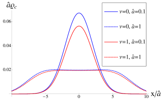
Figure 3: The distribution $\rho_{\rm c}$ along a parallel axis to the x-axis (here at $y=40\widehat{a}^{2}$) is Gaussian shaped for small $\widehat{a}$ (solid curves) and develops a plateau for large lattice spacing (dashed curves).

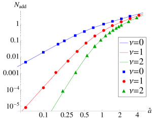
Figure 4: Log-log-plot of the additional real eigenvalues versus $\widehat{a}$ for various $\nu$. The number of matrices and its size vary in this plot for the Monte Carlo simulations (symbols). The statistical error of the numerics varies between $0.1\%$ and $10\%$ around the analytic result (solid curves).

This is shown in Fig. 4. For large lattice spacing the contribution to $N_{\rm add}$ becomes independent of the index $\nu$ whereas for sufficiently small lattice spacing only $\nu=0$ contributes significantly.

For small lattice spacing, the distribution $\rho_{\rm r}$ has a Gaussian shape with a width of $2\widehat{a}$, and for $\widehat{a}\gg 1$, it develops a plateau with sharp edges at $\pm 8\widehat{a}^{2}$, cf. Fig. 6. The height of $\rho_{\rm r}$ at the origin scales like $\widehat{a}^{2\nu+1}$ for small lattice spacing and like $\widehat{a}^{-1}$ for large $\widehat{a}$.

The distribution of chirality over the real eigenvalues $\rho_{\chi}$ is shown in Fig. 6. For small $\widehat{a}$ we observe the spectral density of the $\nu$-dimensional Gaussian unitary ensemble. For large lattice spacing it deforms into a curve with two peaks at $\pm 8\widehat{a}^{2}$ that up to an overall normalization is independent of $\nu$ and evolves into inverse square root singularities for $\widehat{a}\to\infty$.

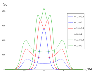
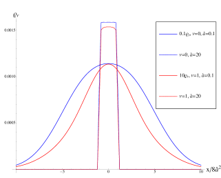
Figure 5: For small lattice spacing (solid curves) the distribution $\rho_{\chi}$ is given by the GUE (See the legend for the values of the index and the lattice spacing). For $\widehat{a}\gg 1$ (dashed curves) the shape becomes $\nu$-independent with two peaks at $\pm 8\widehat{a}^{2}$ that behave as $1/\sqrt{(8\widehat{a}^{2})^{2}-x^{2}}$ for $\widehat{a}\gg 1$.

Figure 6: The eigenvalue distribution $\rho_{\rm r}$ has a Gaussian shape for small $\widehat{a}$ (solid lines) but becomes box like with increasing lattice spacing (dashed curves). Notice that $\rho_{\rm r}$ for ($(\nu,\widehat{a})=(0,0.1)$) and ($(\nu,\widehat{a})=(1,0.1)$) is one order larger and one order smaller than shown in the diagram.

Conclusions.

Discretization effects become strong for $\widehat{a}\approx 0.5$. The oscillations of the spectral density in the continuum limit are no longer visible while the density of the complex eigenvalues develops a plateau with a width of $16\widehat{a}^{2}$. In terms of physical parameters, $\widehat{a}=\widetilde{a}\sqrt{W_{8}V}$, with $W_{8}$ a low energy constant ADSV10b and $V$ the volume of space time, we have the condition that $\widetilde{a}\ll 1/\sqrt{W_{8}V}$ to be close to the continuum limit.

In the regime of small lattice spacing, $\widehat{a}\approx 0.1$, the width of the distribution of the complex eigenvalues is given by $\sigma=2\widetilde{a}\sqrt{W_{8}/V}/\Sigma$ whereas the spacing of the projection of these eigenvalues onto the imaginary axis is equal to $\Delta\lambda=\pi/\Sigma V$. We thus have that $\sigma/\Delta\lambda=2\widehat{a}/\pi$, which allows us to extract a numerical value for $W_{8}$ from lattice simulations.

An important result is that the number of additional real modes is strongly suppressed for large $\nu$. This implies that for large volumes when most configurations have an index $|\nu|>0$, additional real modes are not much of a problem for lattice QCD simulations with Wilson fermions provided that $W_{8}a^{2}V\ll 1$.

References

• (1) J. Feinberg, A. Zee, Nucl. Phys.  B 504, 579 (1997); B. A. Khoruzhenko, H. J. Sommers, The Oxford Handbook of Random Matrix Theory, (2011).
• (2) Y. V. Fyodorov, H. J. Sommers, JETP LETTERS 63, 1026 (1996).
• (3) E. Gudowska-Nowak, G. Papp, J. Brickmann, Chem. Phys. 232, 247 (1998).
• (4) M. A. Stephanov, Phys. Rev. Lett.  76, 4472 (1996); G. Akemann, Int. J. Mod. Phys.  A22, 1077-1122 (2007).
• (5) M. S. Rudner, L. S. Levitov, Phys. Rev. Lett. 102, 065703 (2009).
• (6) E. V. Shuryak, J. J. M. Verbaarschot, Nucl. Phys.  A560, 306-320 (1993).
• (7) G. Akemann, P. H. Damgaard, U. Magnea, S. Nishigaki, Nucl. Phys.  B487, 721-738 (1997).
• (8) J. C. Osborn, Phys. Rev.  D83, 034505 (2011).
• (9) P. H. Damgaard, K. Splittorff and J. J. M. Verbaarschot, Phys. Rev. Lett.  105, 162002 (2010).
• (10) G. Akemann, P. H. Damgaard, K. Splittorff, J. J. M. Verbaarschot, PoS LATTICE2010, 079 (2010); PoS LATTICE2010, 092 (2010); Phys. Rev. D 83, 085014 (2011).
• (11) K. Splittorff, J. J. M. Verbaarschot, [hep-lat/1105.6229], (2011).
• (12) G. Akemann, T. Nagao, [math-ph/1108.3035], (2011).
• (13) S. R. Sharpe and R. L. Singleton, Phys. Rev.  D 58, 074501 (1998).
• (14) G. Rupak and N. Shoresh, Phys. Rev.  66, 054503 (2002).
• (15) S. R. Sharpe, Phys. Rev.  D 74, 014512 (2006).
• (16) S. Necco, A. Shindler, JHEP 1104, 031 (2011).
• (17) L. Del Debbio, L. Giusti, M. Lüscher, R. Petronzio and N. Tantalo, JHEP 0602, 011 (2006); JHEP 0702, 056 (2007).
• (18) G. Akemann, E. Kanzieper, J. Stat. Phys. 129, 1158 (2007); G. Akemann, M. Kieburg, M. J. Phillips, J. Phys. A 43, 375207 (2010).
• (19) K. Splittorff, J. J. M. Verbaarschot, Nucl. Phys.  B683, 467-507 (2004).