Decoherence-free evolution of time-dependent superposition states of two-level systems and thermal effects

Abstract

In this paper we detail some results advanced in a recent letter [Phys. Rev. Lett. 102, 073008 (2009) ] showing how to engineer reservoirs for two-level systems at absolute zero by means of a time-dependent master equation leading to a nonstationary superposition equilibrium state. We also present a general recipe showing how to build nonadiabatic coherent evolutions of a fermionic system interacting with a bosonic mode and investigate the influence of thermal reservoirs at finite temperature on the fidelity of the protected superposition state. Our analytical results are supported by numerical analysis of the full Hamiltonian model.

I Introduction

The purpose of the engineering reservoir program Poyatos is to protect a specific state against the decoherence stemming from the natural coupling between a quantum system and the reservoir. To engineer a reservoir, a given system, whose state is to be protected, is compelled to engage in additional interactions besides that with the natural reservoir. The engineering reservoir technique is then applied to make these additional interactions prevail, modifying the dissipative Liouvillian in a specific way that drives the system to the desired equilibrium with the engineered reservoir. Rightly connected to the engineering Hamiltonian program Fabiano , the reservoir engineering has been developed for trapped ions Ions ; Matos and atomic two-level ($TL$) systems Atoms . Recently, under the assumption of a squeezed engineered reservoir, a way to observe the adiabatic geometric phase acquired by a protected state has been proposed Carollo2006a ; Carollo2006c ; Yin 2007 under the assumption of an adiabatic evolution of the system-reservoir parameters. It is worth mentioning recent results on the possibility to drive an open many-body quantum system into a given pure state by an appropriate design of the system-reservoir coupling Diehl1 ; Diehl2 .

In this paper we detail the general recipe presented in Ref.PRLFabiano09 showing how to build nonadiabatic coherent evolutions of a two-level ion trapped into a leaky cavity, in contrast with the applications of the engineering reservoir technique which require adiabatic conditions Carollo2006a ; Carollo2006c ; Yin 2007 . Furthermore, we show how to implement the proposal of Ref. Carollo2006b for controlling the slow changes of a protected $TL$ system through the parameters of the engineered reservoir. We also investigate the influence of thermal reservoirs at finite temperature on the fidelity of the protected superposition state.

This paper is organized as follows. In Section II we briefly present the engineering reservoir program, including the advances presented in Ref. PRLFabiano09 . In Section III we show in details a general recipe to engineer reservoirs for a fermionic system interacting with a bosonic mode. As an application we derive an effective reservoir for a time-dependent superposition state of the internal degrees of freedom of an ion trapped into a leaky cavity. In Section IV we present numerical results supporting our approximations and an analysis of the temperature effects on the protected time-dependent superposition. Finally, in Section V we present our conclusions.

II The extended engineering reservoir program

Before we present the technique to protect superpositions of quantum states evolving nonadiabatically, we review basics results concerning the engineering reservoir program. To this end, we focus our attention on a system interacting with a reservoir, both system and reservoir being modeled by harmonic oscillators. The coupling, as usual, is assumed to be linear in position-position. From this model one can deduce a master equation, obtained by tracing over the reservoir variables, to study the evolution of the single harmonic oscillator. By driving the system with external fields and/or allowing the system to interact with additional systems, each one possessing its own reservoir, it is possible to obtain, through some approximations, an effective master equation which is the starting point to protect a given state by means of engineered reservoirs, as we detail in the following.

II.1 Protection of a stationary quantum state

The master equation describing the evolution of the density operator $\rho$ of a given system coupled with its natural reservoir in the interaction picture and at zero temperature is

$$\overset{\cdot}{\rho}=\frac{\Gamma}{2}\left(2a\rho a^{\dagger}-a^{\dagger}a\rho-\rho a^{\dagger}a\right),$$ (1)

where $a^{\dagger}$ ($a$) is the creation (annihilation) operator in the Fock states of the system. As it is well known, the only steady state resulting from Eq.(1) is the vacuum $\left|0\right\rangle$, which is an eigenstate of the annihilation operator with zero eigenvalue: $a\left|0\right\rangle=\alpha\left|0\right\rangle$, $\alpha=0$. The main goal of the standard engineering reservoir Poyatos is to obtain, in the interaction picture and at zero temperature, an effective master equation in the form

$$\overset{\cdot}{\rho}=\frac{\Gamma}{2}\left(2\mathcal{O}\rho\mathcal{O}^{\dagger}-\mathcal{O}^{\dagger}\mathcal{O}\rho-\rho\mathcal{O}^{\dagger}\mathcal{O}\right),$$ (2)

where $\Gamma$ is the effective decay rate of the engineered reservoir which is coupled to the quantum system in a specific way characterized by the time-independent system operator $O$. Proceeding in analogy with Eq.(1), the only pure steady state of this system is the eigenstate $\left|\psi\right\rangle$ of the operator $O$ with null eigenvalue, ensuring that there is no further eigenstate $\left|\phi\right\rangle$ of $O$ such that $\left[\mathcal{O},\mathcal{O}^{\dagger}\right]\left|\phi\right\rangle=0$. As a consequence, $\left|\psi\right\rangle$ is the asymptotic state of the system Matos .

II.2 Protection of a time-dependent quantum state

The Ref. PRLFabiano09 adds an improvement on the engineering reservoir program by allowing to remove the adiabatic constraint in the decoherence-free evolution mentioned above. To understand this simple, yet effective improvement, here we review the theory developed in Ref. PRLFabiano09 . Consider the engineered time-dependent master equation in the interaction picture

$$\overset{\cdot}{\rho} =-i\left[H\left(t\right),\rho\right]+\frac{\Gamma}{2}\left[2\mathcal{O}\left(t\right)\rho\mathcal{O}^{\dagger}\left(t\right)-\mathcal{O}^{\dagger}\left(t\right)\mathcal{O}\left(t\right)\rho\right.$$

$$\left.-\rho\mathcal{O}^{\dagger}\left(t\right)\mathcal{O}\left(t\right)\right],$$ (3)

where the Hermitian Hamiltonian $H\left(t\right)$ must be engineered aiming to synthesize —without adiabatic impositions— the desired time-dependence of the operator $\mathcal{O}\left(t\right)=R\left(t\right)\mathcal{O}_{R}R^{{\dagger}}\left(t\right)$, with $\overset{\cdot}{\mathcal{O}}_{R}=0$, $R\left(t\right)=T\exp\left(-i\int_{0}^{t}H\left(t^{\prime}\right)dt^{\prime}\right)$, and $T$ being the time-ordering operator. Such a relation between $\mathcal{O}\left(t\right)$ and $R(t)$ justifies the above mentioned intimate connection between both programs of engineering Hamiltonians and reservoirs; in fact, the reservoir engineering technique relies on engineered Hamiltonians. We stress that we have achieved the time evolution of Eq. (3) in a particular way that the engineered Hamiltonian $H\left(t\right)$ prompts the specific operator $O\left(t\right)$ and its protected evolving eigenstate $\left|\psi\left(t\right)\right\rangle$ (with null eigenvalue). The key feature to be noted here is that, through the unitary transformation $R\left(t\right)$, we recover the time-independent form of the master equation:

$$\overset{\cdot}{\rho_{R}}=\frac{\Gamma}{2}\left(2\mathcal{O}_{R}\rho_{R}\mathcal{O}_{R}^{\dagger}-\mathcal{O}_{R}^{\dagger}\mathcal{O}_{R}\rho_{R}-\rho_{R}\mathcal{O}_{R}^{\dagger}\mathcal{O}_{R}\right).$$ (4)

Therefore, the protected stationary state, $\left|\psi_{R}\right\rangle$ ($\mathcal{O}_{R}\left|\psi_{R}\right\rangle=0$), turns out to be a nonstationary state $\left|\psi(t)\right\rangle=R\left(t\right)\left|\psi_{R}\right\rangle$ in the original interaction picture of (3), where $H\left(t\right)=i\overset{\cdot}{R}(t)R^{{\dagger}}(t)$. Getting rid of the adiabatic constraints, we are thus allowed to manipulate the evolution of the protected state $\left|\psi(t)\right\rangle$ through appropriate engineered Hamiltonian and reservoir. It is worth mention that the time dependence of the protected state is closely related to the properties of $H(t)$ and $O\left(t\right)$. If $\left[H(t),\mathcal{O}\left(t\right)\right]=\left[i\overset{\cdot}{R}(t)R^{{\dagger}}(t),\mathcal{O}\left(t\right)\right]=i$ $\overset{\cdot}{\mathcal{O}}\left(t\right)=0$, then it is straightforward to see that $\left|\psi(t)\right\rangle=\left|\psi_{R}\right\rangle$, i.e., $\left|\psi(t)\right\rangle\,$is stationary apart from a global phase factor.

Next we develop a general theory of reservoir engineering for a system interacting with a bosonic mode, i. e., we show how to use the bosonic decay to build up the general master equation (2). Then we apply this theory to protect quantum states of a $TL$ system, showing how to obtain an effective interaction between this system and a cavity mode which leads to the desired state protection mechanism.

III Reservoir engineering for a fermionic system interacting with a dissipative bosonic field

The starting point to develop a general theory of reservoir engineering for a fermionic system (from now on ”the system”) interacting with a dissipative bosonic field is the engineered effective Hamiltonian

$$H_{eff}=\lambda_{eff}\left(\mathfrak{O}a^{\dagger}+\mathfrak{O}^{\dagger}a\right),$$ (5)

where $a^{\dagger}$ ($a$) is the creation (annihilation) operator of the bosonic field, while $\mathfrak{O}$ and $\mathfrak{O}^{\dagger}$ are operators associated with the system whose state we wish to protect, and $\lambda_{eff}\$is the effective coupling between the bosonic mode and the system. As an example, some of us showed how to build up bimodal interactions in cavity quantum electrodynamics using three- or two-level atoms Fabiano . We note that the interaction (5) is a bilinear form similar to the interaction of a bosonic field with a natural reservoir which leads to the well-know Liouvillian describing the amplitude damping mechanism. Thus, the engineered interaction (5) must generate an effective dissipative Liouvillian which competes with the natural one. When the engineered decay rate is significantly larger than the natural one, the effective dissipative Liouvillian will govern the dynamics of the system.

Once achieved the important step of building the interaction between the system of interest and the quantized bosonic mode, we now add the dissipative mechanism of the bosonic mode through the master equation

$$\overset{\cdot}{\rho^{(sa)}} =-i\left[H_{eff},\rho^{(sa)}\right]$$

$$+\frac{\kappa}{2}\left(2a\rho^{(sa)}a^{\dagger}-a^{\dagger}a\rho^{(sa)}-\rho^{(sa)}a^{\dagger}a\right),$$ (6)

written in the same representation we obtained $H_{eff}$; the factor $\kappa$ stands for the natural decay rate of the bosonic mode and the supra index in $\rho^{(sa)}$ indicates its dependence from both the field ($a$) and system ($s$) operators. From the above equation we straightforwardly derive the evolution equation for the matrix elements $\rho_{nm}^{(s)}=\left\langle n\right|\rho^{(sa)}\left|m\right\rangle$ in the Fock basis:

$$\overset{\cdot}{\rho}_{n,m}^{(s)} =-i\lambda_{eff}\left[\sqrt{n}\mathfrak{O}\rho_{n-1,m}^{(s)}+\sqrt{n+1}\mathfrak{O}^{\dagger}\rho_{n+1,m}^{(s)}\right.$$

$$\left.-\left(\sqrt{m+1}\rho_{n,m+1}^{(s)}\mathfrak{O}+\sqrt{m}\rho_{n,m-1}^{(s)}\mathfrak{O}^{\dagger}\right)\right]$$ (7)

$$+\kappa\sqrt{\left(n+1\right)\left(m+1\right)}\rho_{n+1,m+1}^{(s)}-\frac{\kappa}{2}\left(n+m\right)\rho_{n,m}^{(s)}.$$

To engineer the reservoir, we assume that the decay constant $\kappa$ of the bosonic mode is significantly larger than the effective coupling $\lambda_{eff}$ in Eq. (7). This condition is easily achieved for cavities with low quality factor $Q=\omega/\kappa$, where $\omega$ is the bosonic mode frequency. Together with the good approximation of a reservoir at zero temperature, this regime enables to consider only the matrix elements $\rho_{mn}^{(s)}$ inside the subspace $\left\{\left|0\right\rangle\text{,}\left|1\right\rangle\right\}$ of Fock states. Actually, Eq. (7) can very well be described by the set of equations

$$\overset{\cdot}{\rho}_{0,0}^{(s)}=-i\lambda_{ef}\left(\mathfrak{O}^{\dagger}\rho_{1,0}^{(s)}-\rho_{0,1}^{(s)}\mathfrak{O}\right)+\kappa\rho_{1,1}^{(s)},$$ (8)

$$\overset{\cdot}{\rho^{(s)}}_{1,0}=\left(\overset{\cdot}{\rho}_{0,1}\right)^{\dagger}=-i\lambda_{ef}\left(\mathfrak{O}\rho_{0,0}^{(s)}-\rho_{1,1}\mathfrak{O}\right)-\frac{\kappa}{2}\rho_{1,0}^{(s)},$$ (9)

$$\overset{\cdot}{\rho}_{1,1}^{(s)}=-i\lambda_{ef}\left(\mathfrak{O}\rho_{0,1}^{(s)}-\rho_{1,0}^{(s)}\mathfrak{O}^{\dagger}\right)-\kappa\rho_{1,1}^{(s)},$$ (10)

which are similar to those written in the atomic basis in the reservoir engineering program for trapped ions Matos . The strong decay rate $\kappa$ enables the adiabatic elimination of the elements $\rho_{01}$ and $\rho_{11}$ from the equations above. The formal adiabatic elimination is equivalent to assume $\overset{\cdot}{\rho^{(s)}}_{1,0}\simeq 0$, allowing us to write $\rho_{1,0}^{(s)}=-i2\frac{\lambda_{ef}}{\kappa}\left(\mathfrak{O}\rho_{0,0}^{(s)}-\rho_{1,1}\mathfrak{O}\right)$. We can thus eliminate both $\rho_{1,0}^{(s)}$ and $\widetilde{\rho}_{0,1}^{(s)}$ from the dynamics of the diagonal elements of the density matrix by substituting them in the above equations. Since $\rho_{0,0}^{(s)}+\rho_{1,1}^{(s)}\simeq\rho^{(s)}\equiv\rho_{sys}$, the reduced density operator for the system of interest thus results

$$\overset{\cdot}{\rho_{sys}}=\frac{\Gamma_{eng}}{2}\left(2\mathfrak{O}\rho_{sys}\mathfrak{O}^{{\dagger}}-\mathfrak{O}^{\dagger}\mathfrak{O}\rho_{sys}-\rho_{sys}\mathfrak{O}^{\dagger}\mathfrak{O}\right)\text{,}$$ (11)

where $\Gamma_{eng}=4\lambda_{eff}^{2}/\kappa$ represents the effective decay rate corresponding to the engineered reservoir. With this result we can easily see that the reservoir engineering technique depends basically on the manipulation of the interaction between the bosonic mode and the system whose state we wish to protect.

The two kinds of master equations presented above, (2) and (3), may be recovered through Eq. (11) by identifying the operator $\mathfrak{O}$ with $O$ and $O_{R}$, respectively. Such correspondence is established when the operator $O$ is written in the usual interaction picture, while $O_{R}$ is written in an arbitrary representation where it is stationary and Eq. (3) remains valid. Below we show how to engineer a reservoir which allows to protect an arbitrary evolving superposition state of the internal degrees of freedom of a trapped ion/atom without the adiabatic constraints.

III.1 Engineering reservoirs for a two-level system in a leaky cavity

To implement the ideas discussed in the previous Section, we use a two-level ($TL$) system (s) characterized by the transition frequency $\omega_{0}$ between the ground $\left|g\right\rangle$ and excited $\left|e\right\rangle$ states. This system can be either a $TL$ neutral atom in a dipole trap rempe-kimble or a $TL$ ion in a harmonic trap with frequency $\nu$ blatt . The transition $\left|g\right\rangle$ $\leftrightarrow$ $\left|e\right\rangle$ is driven by a classical field of frequency $\omega_{c}$, with coupling strength $\Omega_{c}$. The $TL$ system is made to interact with a cavity mode field ($a$) of frequency $\omega_{a}$ under the Jaynes-Cummings Hamiltonian with Rabi frequency $g$. Assuming the case of a two-level trapped ion, the Hamiltonian modelling this system is given, within the rotating-wave approximation ($RWA$), by

$$H=\omega_{a}a^{\dagger}a+\omega_{0}\sigma_{z}/2+\nu b^{\dagger}b+\left\{g\cos\left(\overrightarrow{k}.\overrightarrow{x}\right)a\sigma_{eg}\right.$$

$$\left.+\Omega_{c}\operatorname*{e}\nolimits^{i\left(\overrightarrow{k}_{c}.\overrightarrow{x}+\phi_{c}-\omega_{c}t\right)}\sigma_{eg}+\mathrm{H{.c.}}\right\},$$ (12)

where $b^{\dagger\text{ }}$($b$) is the creation (annihilation) operator of the vibrational mode whose position operator is $\overrightarrow{x}=(b^{\dagger}+b)/\sqrt{2m\nu}\widehat{x}$, $m$ being the ionic mass and $\widehat{x}$ the unit vector along the vibrational direction. The wave vectors $\overrightarrow{k}$ and $\overrightarrow{k}_{c}$ stand for the cavity mode and the classical amplification field (with relative phase $\phi_{c}$), respectively, while $\sigma_{rs}\equiv\left|r\right\rangle\left\langle s\right|$ ($r$ and $s$ labeling the states $g$ or $e$). The vibrational mode is decoupled from the remaining degrees of freedom of our model by assuming the wave vectors $\overrightarrow{k}$ and $\overrightarrow{k}_{c}$ to be perpendicular to $\overrightarrow{x}$; otherwise, a sufficiently small Lamb-Dicke parameter keeps the motional state almost unchanged. Under this assumption we arrive at the Hamiltonian

$$H=\omega_{a}a^{\dagger}a+\frac{\omega_{0}}{2}\sigma_{z}+\left\{ga\sigma_{eg}+\Omega_{c}\operatorname{e}^{i\left(\phi_{c}-\omega_{c}t\right)}\sigma_{eg}+\mathrm{H{.c.}}\right\}\text{,}$$ (13)

which will be the starting point for our purposes. In the following, we show how to engineer reservoirs suitable for obtaining nonadiabatic evolutions of the internal ionic states.

III.1.1 Nonadiabatic Evolution

To engineer the appropriate interaction between the $TL$ ion and the cavity mode we apply the unitary transformation given by $U_{1}=\exp\left[-i\left(\omega_{a}a^{\dagger}a+\omega_{c}\sigma_{z}/2\right)t\right]$, leading to the Hamiltonian

$$H_{1}=\frac{\Delta_{c}}{2}\sigma_{z}+\left[\left(\left|\Omega_{c}\right|\operatorname{e}^{i\phi_{c}}+g\operatorname{e}^{-i\delta_{a}t}a\right)\sigma_{eg}+\mathrm{H{.c.}}\right],$$

with $\Delta_{c}=\omega_{0}-\omega_{c}$ ($\delta_{a}=\omega_{a}-\omega_{c}$) being the detuning between the atomic transition (cavity mode) and the laser field. Moving to another frame of reference defined by the unitary transformation $U_{2}=\exp\left\{-i\left[\left(\Delta_{c}/2\right)\sigma_{z}+\left|\Omega_{c}\right|\left(\sigma_{eg}\operatorname{e}^{i\phi_{c}}+\sigma_{ge}\operatorname{e}^{-i\phi_{c}}\right)\right]t\right\},$ the foregoing calculations are significantly simplified. This procedure leads to the Hamiltonian

$$H_{2} =g\operatorname{e}^{-i\delta_{a}t}a\left[\lambda\left(\sigma_{++}-\sigma_{--}\right)+\right.$$

$$\left.\lambda_{+-}\operatorname{e}^{i2\xi t}\sigma_{+-}+\lambda_{-+}\operatorname{e}^{-i2\xi t}\sigma_{-+}\right]\operatorname{e}^{-i\phi_{c}}+\mathrm{H{.c.}}\text{,}$$ (14)

where $\lambda=\sqrt{4-\chi^{2}}/4$, $\lambda_{\pm\mp}=\mp\left(2\pm\chi\right)/4$, and $\xi=\sqrt{\left|\Omega_{c}\right|^{2}+\Delta_{c}^{2}/4}$. The atomic operators are defined by $\sigma_{\pm\pm}=\left|\pm\right\rangle\left\langle\pm\right|$, with $\left|\pm\right\rangle=\frac{1}{2}\left(\sqrt{2\pm\chi}\left|e\right\rangle\pm\operatorname{e}^{-i\phi_{c}}\sqrt{2\mp\chi}\left|g\right\rangle\right)$ and $\chi=\Delta_{c}/\xi$. By assuming a large detuning between the cavity mode and the laser field, such that $\delta_{a}\gg g$, together with the additional choice $\delta_{a}=-2\xi$, we obtain under the RWA the effective Hamiltonian

$$H_{eff}=g_{eff}\left(\operatorname{e}^{i\phi_{c}}\sigma_{+-}a^{\dagger}+\operatorname{e}^{-i\phi_{c}}\sigma_{-+}a\right),$$ (15)

with $g_{eff}=g\left(1-\chi/2\right)/2$. The effective coupling thus depends on the parameter $\chi$, whose value follows from the laser detuning $\Delta_{c}$ which must be significantly smaller than the Rabi frequency $\Omega_{c}$.

Next, observing that $\chi\in\left[-2,2\right]$, we focus on the values $\chi\ll 2$ which allow for an effective coupling of the same order of the atom-cavity field coupling, i.e., $g_{eff}\left(\chi\right)\sim g$. Once achieved the building of the interaction between the two-level system and the cavity mode, we now take into account their interaction with a thermal reservoir at temperature $T=0K$ through the master equation

$$\overset{\cdot}{\widetilde{\rho}^{(sa)}} =-i\left[H_{eff},\widetilde{\rho}^{(sa)}\right]$$

$$+\frac{\kappa}{2}\left(2a\widetilde{\rho}^{(sa)}a^{\dagger}-a^{\dagger}a\widetilde{\rho}^{(sa)}-\widetilde{\rho}^{(sa)}a^{\dagger}a\right)$$ (16)

$$+\frac{\gamma}{2}\left(2\widetilde{\sigma}_{ge}\widetilde{\rho}^{(sa)}\widetilde{\sigma}_{eg}-\widetilde{\sigma}_{ee}\widetilde{\rho}^{(sa)}-\widetilde{\rho}^{(sa)}\widetilde{\sigma}_{ee}\right),$$

where again the supra index in $\widetilde{\rho}^{(sa)}$ denotes the density operator for both system and field and the tilde is used to describe the operators in the same representation of $H_{eff}$, i.e., $\widetilde{\mathcal{O}}=U_{2}^{\dagger}U_{1}^{\dagger}OU_{1}U_{2}$. Here the constants $\kappa$ and $\gamma$ are the decay rates of the cavity mode and the TL system, respectively. Now, except by the superoperator describing the decay of the two-level system, we can see that Eq. (16) is equivalent to Eq. (6), with $\lambda_{eff}=g_{eff}$ and $\mathfrak{O}=\operatorname{e}^{i\phi_{c}}\sigma_{+-}$ . As described above, assuming a strong decay rate $\kappa$ we can adiabatically eliminate the cavity mode variables. This procedure is needed to make clear what is the asymptotically protected atomic superposition. Then, the dynamics of the reduced density operator for the $TL$ system results to be ($\widetilde{\rho}^{(s)}\equiv\widetilde{\rho}_{at}$)

$$\overset{\cdot}{\widetilde{\rho}}_{at}\simeq\frac{\Gamma_{eng}}{2}\left(2\sigma_{+-}\widetilde{\rho}_{at}\sigma_{-+}-\sigma_{--}\widetilde{\rho}_{at}-\widetilde{\rho}_{at}\sigma_{--}\right)+\widetilde{\mathcal{L}}\widetilde{\rho}_{at}\text{,}$$ (17)

so that $\Gamma_{eng}=4g_{eff}^{2}/\kappa$ represents the effective damping of the engineered reservoir and $\widetilde{\mathcal{L}}\widetilde{\rho}_{at}$ is the last term in the r.h.s. of Eq. (16) after tracing over the cavity field variables. Note that the operator $\sigma_{+-}$ and consequently the protected state $\left|+\right\rangle$ ($\sigma_{+-}\left|+\right\rangle=0$), exhibit no temporal dependences in the convenient representation where we have described the evolution (17). However, as we shall see in the following, a coherent nonadiabatic evolution is recovered in the interaction picture, where $\left|+\left(t\right)\right\rangle=UU_{1}U_{2}\left|+\right\rangle$ and $U=\exp\left[i\left(\omega_{a}a^{\dagger}a+\omega_{0}\sigma_{z}/2\right)t\right]$, even under spontaneous decay, provided that $\gamma\ll\Gamma_{eng}$. Here we note that the combined unitary operations $UU_{1}U_{2}$ act on the Hilbert space of the atom and the mode. However, once we are interested in the two-level system only and since the field and atomic operators commute with each other, we are omitting, for convenience, the corresponding state of the mode.

Ideal case: In the ideal case where $\gamma=0$, the solution of Eq. (17) leads to the $TL$ steady state $\widetilde{\rho}_{at}=$ $\left|+\right\rangle\left\langle+\right|$. By returning to the interaction picture we thus obtain $\rho_{at}=\left|+\left(t\right)\right\rangle\left\langle+\left(t\right)\right|$, where

$$\left|+\left(t\right)\right\rangle=\frac{1}{2}\left(\sqrt{2+\chi}\left|e\right\rangle+\operatorname{e}^{-i\Phi(t)}\sqrt{2-\chi}\left|g\right\rangle\right),$$ (18)

with $\Phi(t)=\phi_{c}-\Delta_{c}t$. This state describes a nonadiabatic evolution that depends on the detuning $\Delta_{c}$ between the atomic transition and the classical field. Note that under the restriction $\chi\ll 2$ imposed above, the states around the north pole of the Bloch sphere are not allowed steady states.

Nonideal case: To appreciate the robustness of the present reservoir engineering technique, it is necessary to take into account the damping stemming from the natural reservoir when $\gamma\neq 0$. Here we will consider the reservoir at zero temperature. The effect of finite temperature in the fidelity of the protected state will be analyzed in the next Section. For convenience, we will analyze such effects in the frame on which we have defined $H_{1}$. To this end, we use $\widetilde{\rho}_{at}=U_{2}^{\dagger}\rho_{at}U_{2}$ in Eq. (17), which can thus be written as

$$\overset{\cdot}{\rho_{at}} =-i\left[\xi\left(\sigma_{++}-\sigma_{--}\right),\rho_{at}\right]$$

$$+\frac{\Gamma_{eng}}{2}\left(2\sigma_{+-}\rho_{at}\sigma_{-+}-\sigma_{--}\rho_{at}-\rho_{at}\sigma_{--}\right)$$ (19)

$$+\frac{\gamma}{2}\left(2\sigma_{ge}\rho_{at}\sigma_{eg}-\sigma_{ee}\rho_{at}-\rho_{at}\sigma_{ee}\right)\text{.}$$

By projecting Eq. (19) on the atomic basis we find the following set of equations corresponding to the matrix elements $\rho_{at}^{++}\equiv\left\langle+\right|\rho_{at}\left|+\right\rangle$ , $\rho_{at}^{+-}\equiv\left\langle+\right|\rho_{at}\left|-\right\rangle$, and $\rho_{at}^{-+}\equiv\left\langle-\right|\rho_{at}\left|+\right\rangle$:

$$\overset{\cdot}{\rho}_{at}^{++} =\left.\Gamma_{eng}+\widetilde{\gamma}\left(\chi^{2}-2\right)-\left[\Gamma_{eng}+2\widetilde{\gamma}\left(\chi^{2}+4\right)\right]\rho_{at}^{++}\right.$$

$$\left.-\widetilde{\gamma}\chi\sqrt{4-\chi^{2}}\left(\rho_{at}^{+-}+\rho_{at}^{-+}\right)\right.\text{,}$$

$$\overset{\cdot}{\rho}_{at}^{+-} =\left.\widetilde{\gamma}\left(\chi^{2}-2\right)-2\widetilde{\gamma}\chi\sqrt{4-\chi^{2}}\rho_{at}^{++}\right.$$

$$\left.-\left[\frac{\Gamma_{eng}}{2}+2\widetilde{\gamma}\left(\chi^{2}-12\right)-i2\xi\right]\rho_{at}^{+-}\right.$$

$$\left.+\widetilde{\gamma}\sqrt{4-\chi^{2}}\rho_{at}^{-+}\right.\text{,}$$

with $\widetilde{\gamma}=\gamma/16$. Imposing the condition $\overset{\cdot}{\rho}_{at}=0$, we can also determine the asymptotic solutions for $\rho_{at}^{++}$ and $\rho_{at}^{+-}$, greater simplified considering a large cooperative parameter $\mathcal{C}=g^{2}/\gamma\kappa\simeq\Gamma_{eng}/\gamma\gg 1$, given by

$$\rho_{++} =1-\epsilon_{++}\text{ ,}$$

$$\rho_{+-} =-i\epsilon_{+-}\text{,}$$

where $\epsilon_{++}=\left(\gamma/\Gamma_{eng}\right)\left[\left(2+\chi\right)/8\right]^{2}$ and $\epsilon_{+-}=\gamma/4g_{eff}$. Under the condition $\Gamma_{eng}/\gamma\gg 1$, we see that both $\epsilon_{++}$ and $\epsilon_{+-}$ are much smaller than unity. Actually, taking into account the noise effects introduced by the reservoir, the steady state is approximately described by $\rho_{at}\simeq\left|+\right\rangle\left\langle+\right|$. The net effect of the noise introduced by the atomic decaying mechanism is computed through the fidelity

$$\mathcal{F}=\mathrm{Tr}\left[\left|+\right\rangle\left\langle+\right|\rho_{at}\right]=1-\epsilon_{++}\text{.}$$

The approximation leading to Eq. (19) is better as higher the decay rate $\kappa$; however, for the dynamics of the $TL$ system to be driven by the engineered reservoir, the magnitude of $\kappa$ must be chosen within the restriction $\mathcal{C}\gg 1$. Within the optical regime Hood , for example, where $g\simeq 7\times 10^{8}$ s^-1 and $\gamma\simeq 2\times 10^{7}$ s^-1, we obtain for a cavity decay constant $\kappa\simeq 3g$, the strength $\kappa/\gamma\simeq 10$ and a fidelity around $96\%$. Therefore, under the excellent approximation $\epsilon_{++}\ll 1$ and reversing the unitary transformation $R(t)$, the state $\left|+\right\rangle$, written in the interaction picture Eq. (18) allows for a nonadiabatic coherent evolution of a $TL$ system under spontaneous decay, which can be manipulated through the parameter $\Delta_{c}$. Such an evolution corresponds to flips in the atomic states, representing trajectories on different planes parallel to the equator on the Bloch sphere, governed by the Hamiltonian $H=\Omega_{c}\sigma_{eg}\operatorname*{e}\nolimits^{-i(\Delta_{c}t-\phi_{c})}+H.c.$.

IV Numerical results and temperature effects

To validate the approximations carried out in the previous Section, we proceed to numerically evaluate the full Hamiltonian Eq. (13), in the interaction picture, taking into account the thermal reservoir for both the atom and the field, such that

$$\overset{\cdot}{\rho^{(sa)}} =-i\left[V,\rho^{(sa)}\right]$$

$$+\frac{\kappa\left(\overline{n}_{a}+1\right)}{2}\left(2a\rho^{(sa)}a^{\dagger}-a^{\dagger}a\rho^{(sa)}-\rho^{(sa)}a^{\dagger}a\right)$$

$$+\frac{\kappa\overline{n}_{a}}{2}\left(2a^{\dagger}\rho^{(sa)}a-aa^{\dagger}\rho^{(sa)}-\rho^{(sa)}aa^{\dagger}\right)$$

$$+\frac{\gamma\left(\overline{n}_{s}+1\right)}{2}\left(2\sigma_{ge}\rho^{(sa)}\sigma_{eg}-\sigma_{ee}\rho^{(sa)}-\rho^{(sa)}\sigma_{ee}\right)$$

$$+\frac{\gamma\overline{n}_{s}}{2}\left(2\sigma_{eg}\rho^{(sa)}\sigma_{ge}-\sigma_{gg}\rho^{(sa)}-\rho^{(sa)}\sigma_{gg}\right)\text{,}$$ (20)

where

$$V=ga\sigma_{eg}\operatorname{e}^{-i\delta_{a}t}+\Omega_{c}\sigma_{eg}\operatorname{e}^{i\left(\phi_{c}-\Delta_{c}t\right)}+\mathrm{H{.c.}}\text{,}$$

and $\overline{n}_{a}$ and $\overline{n}_{s}$ are the average number of thermal photons for the bosonic field and atomic reservoirs, respectively.

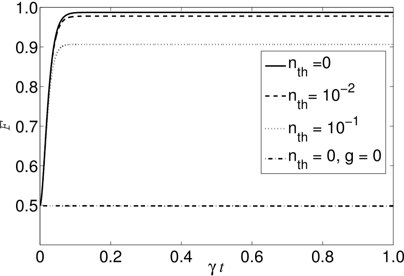
Figure 1: Evolution of the numerically computed fidelity for both cases of absolute zero (solid line) and finite temperature, with the average number of thermal photons $\overline{n}=0.01$ (dashed line) and $\overline{n}=0.1$ (dotted line). The constant value $\mathcal{F}=0.5$ indicated by the dashed-dotted line refers to the case where the coupling $g$ between the atomic system and the cavity mode is null.

We emphasize that, differently from the master equation (16) which has been derived under the RWA approximation leading to the effective Hamiltonian (15), the above master equation (20) describes exactly the dynamics of the whole system thus allowing us to quantify the errors introduced by our approximations – RWA in Eq. (15) and adiabatic elimination of the field variables in Eq. (17). Since we are assuming the atomic frequency near the resonance with the cavity field frequency, both their reservoirs will have the same average thermal photons, such that from now on we take $\overline{n}_{a}$ $=$ $\overline{n}_{s}$. By projecting the above equation in the Fock $\left\{\left|n\right\rangle\right\}$ and electronic $\left\{\left|e\right\rangle,\left|g\right\rangle\right\}$ bases, we are lead to an infinity set of coupled equations for the matrix elements. To solve numerically this system of infinity coupled differential equations we must truncate the Fock basis somewhere. The strong decay rate $\kappa$ allows us to safely do it since the matrix elements corresponding to highly excited Fock states are virtually zero. We then numerically solve the master equation (20) following the method presented in master-matlab . Since we are interested in the evolution of the atomic two-level system only, we trace numerically over the bosonic field variables. Therefore, after solving the full master equation we end up with a density matrix for the two-level system with elements

$$\rho_{at}^{ij}\left(t\right)=\sum_{n=0}^{N}\rho_{n,n}^{ij}\left(t\right)\text{,}$$ (21)

where $\rho_{at}^{ij}\equiv\left\langle i\right|\rho_{at}\left|j\right\rangle$.

Here we analyze the robustness of the protected atomic superposition given by Eq. (18). Our strategy consists in computing the robustness of the protected state under thermal effects considering the following different regimes: i) $\Phi(t)=$ constant, which corresponds to the static case, ii) by allowing $\Phi(t)$ to slowly vary with time, corresponding to $\Delta_{c}/\Gamma_{eng}\ll 1$, and iii) allowing $\Delta_{c}(t)$ to rapidly vary in time, corresponding to $\Delta_{c}/\Gamma_{eng}>1$. The robustness of the protected state is computed through the fidelity $\mathcal{F}(t)=\mathrm{Tr}\left[\left|+(t)\right\rangle\left\langle+(t)\right|\rho_{at}(t)\right]$ where $\rho_{at}(t)$ follows from the numerical solution of the full master equation (20). In units of $\gamma$, we assumed the reasonable decay rates $\kappa=10^{2}\gamma$, $g=10^{2}\gamma$ and $\Omega_{c}=2\times 10^{3}\gamma$.

Starting with the static case, we consider $\Delta_{c}(t)=0$ with constant $\phi_{c}$, such that $\left|+\right\rangle=\frac{1}{\sqrt{2}}\left(\left|e\right\rangle+\operatorname{e}^{i\phi_{c}}\left|g\right\rangle\right)$. Assuming $\phi_{c}=0$ and the $TL$ atom prepared in the ground state, in Fig. 1 we present the numerical results of the fidelity against the parameter $\gamma t$ for both cases of absolute zero (solid line) and finite temperature, with the average number of thermal photons $\overline{n}=0.01$ (dashed line) and $\overline{n}=0.1$ (dotted line). As expected, we verify that the temperature effects reduce substantially the fidelity of the atomic superposition. To stress the effectiveness of our protocol, we call the attention to the case where the coupling $g$ between the atomic system and the cavity mode is null. In this case we observe that the fidelity remains $\mathcal{F}=0.5$ (dashed-dotted line) showing that the cavity mode is a crucial ingredient, together with the classical pumping, to protect the desired superposition state.

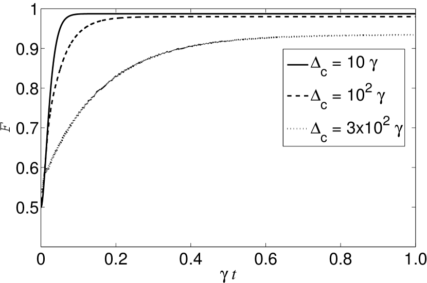
Figure 2: Fidelity of the protected state $\left|+\left(t\right)\right\rangle$ undergoing adiabatic and nonadiabatic evolutions at zero temperature. We consider the values $\Delta_{c}/\Gamma_{eng}\simeq 0.1$ (solid line), $\Delta_{c}/\Gamma_{eng}\simeq 1$ (dashed line), and finally, $\Delta_{c}/\Gamma_{eng}\simeq 3$ (dotted line).

In Fig. 2 we plot the fidelity of the protected state $\left|+\left(t\right)\right\rangle$ undergoing slow and fast evolutions. We have considered three distinct values for the detuning between the atom and the classical field: $\Delta_{c}=10\gamma$, leading to a slow evolution with $\Delta_{c}/\Gamma_{eng}\simeq 0.1$ (solid line), $\Delta_{c}=10^{2}\gamma$, departing from the adiabatic regime with $\Delta_{c}/\Gamma_{eng}\simeq 1$ (dashed line), and finally $\Delta_{c}=3\times 10^{2}\gamma$, with $\Delta_{c}/\Gamma_{eng}\simeq 3$ (dotted line). All these curves in Fig. 2 were plotted considering $\overline{n}=0$. As we are concerned with slow and fast evolutions dictated by the time varying parameter $\Phi(t)=\phi_{c}-\Delta_{c}t$, we focused our attention in $\Delta_{c}(t)$ taking $\phi_{c}=0$. We stress that when the condition $\Delta_{c}/\Gamma_{eng}\ll 1$ is weakened, meaning that some parameters are rapidly varying in time, we found that although the equilibrium is reached more slowly, the fidelity does not drop off quickly, attaining a value about $0.9$ even for $\Delta_{c}/\Gamma_{eng}\simeq 3$, corroborating again the effectiveness of our protocol.

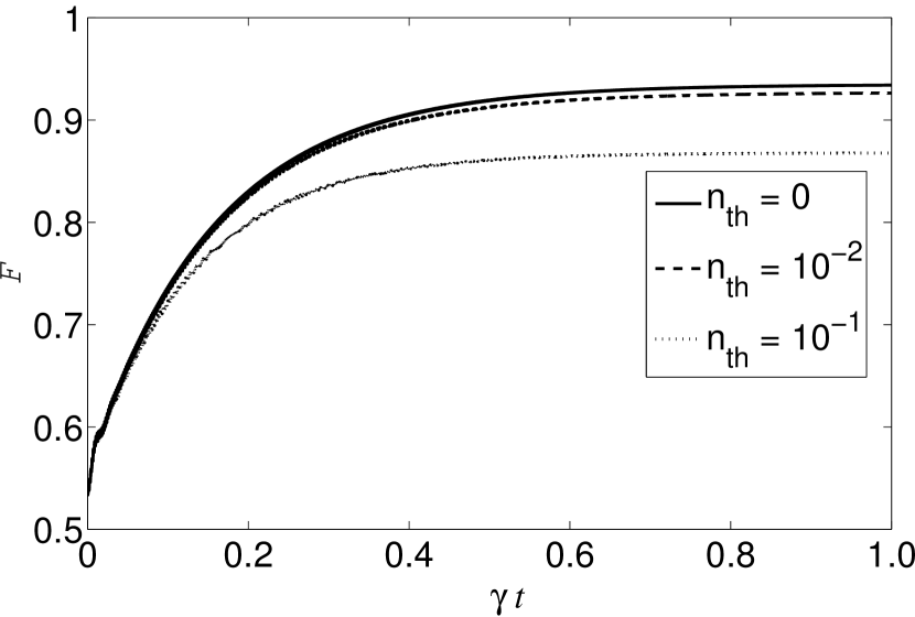
Figure 3: Fidelity of the protected state $\left|+\left(t\right)\right\rangle$ undergoing nonadiabatic evolutions, with $\Delta_{c}=3\times 10^{2}\gamma$ ($\Delta_{c}/\Gamma_{eng}\simeq 3$), for absolute zero (solid line) and finite temperature, with the average number of thermal photons $\overline{n}=0.01$ (dashed line) and $\overline{n}=0.1$ (dotted line).

In order to see the temperature effects in the nonadiabatic evolutions, in Fig. 3 we draw the curves of the fidelity for $\Delta_{c}=3\times 10^{2}\gamma$ ($\Delta_{c}/\Gamma_{eng}\simeq 3$) for different values of mean number of thermal photons, i.e., for absolute zero (solid line), $\overline{n}=0.01$ (dashed line) and $\overline{n}=0.1$ (dotted line). Again, as in the static case (Fig. 1), we observe that the fidelity decreases with the increase of the mean number of thermal photons, showing that the temperature is the most important source of decoherence in our present protocol. This conclusion is also drawn from Fig.4, where a functional dependence of the fidelity of the protected state $\left|+\left(t\right)\right\rangle$ undergoing nonadiabatic evolutions against the reservoirs mean photon number is displayed. From this figure, where we have used $g=10\gamma$ (solid line), $20\gamma$(dashed line), $50\gamma$ (dotted) and $10^{2}\gamma$ (dashed-dotted line), we note that the fidelity decays faster with the increasing number of thermal photons, as we have mentioned above.

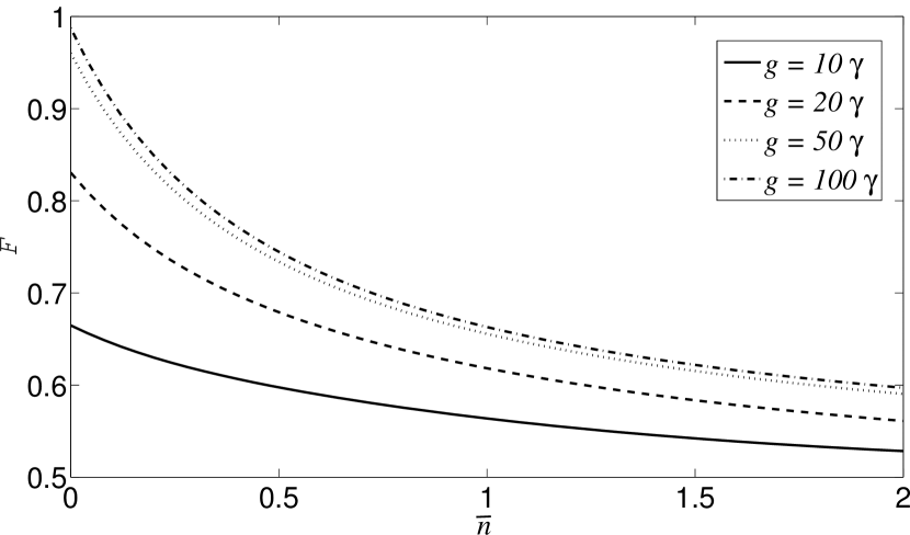
Figure 4: Fidelity of the protected state $\left|+\left(t\right)\right\rangle$ undergoing nonadiabatic evolutions, versus the average thermal photons $\overline{n}$ characterizing the finite temperatures with $g=10\gamma$ (solid line), $20\gamma$(dashed line), $50\gamma$ (dotted) and $10^{2}\gamma$ (dashed-dotted line).

V Concluding Remarks

In this paper we deepened the analysis of the engineering reservoir technique we have proposed in Ref. PRLFabiano09 . This proposal has been accomplished by deriving a time-dependent master equation which leads to a decoherence-free evolving superposition state which can be nonadiabatically controlled by the system-reservoir parameters. In the present contribution we have provided a general recipe to engineer arbitrary effective reservoirs for a fermionic system by manipulating its interaction with a bosonic mode.

More specifically, we showed how to protect a superposition state of a two-level ion trapped into a leaky cavity. The robustness of our scheme was analyzed by means of the fidelity considering the case where the protected state does not depend on time, as well as the case of slowly and rapidly time varying evolutions. To support the approximations used to derive our analytical results, we have numerically solved the full master equation, obtaining an excellent agreement with the approximations we have carried out. In the present contribution we also analyzed the temperature effects of the reservoirs on the fidelity of the static and time varying protected states. We concluded that the temperature is the most important source of decoherence in our present protocol.

We hope that this contribution can be useful for information processing with trapped ions inside optical cavities, for example for implementing Deutsch algorithm deutsch ; eduardo or universal dissipative quantum computing cirac-naturephysics .

We wish to express our thanks to FAPESP, FAPEMIG, CAPES, CNPq, and the Brazilian National Institute of Science and Technology for Quantum Information (INCT-IQ), for the financial support.

References

- (1) J. F. Poyatos, J. I. Cirac, and P. Zoller, Phys. Rev. Lett. 77, 4728 (1996).
- (2) F. O. Prado, N. G. de Almeida, M. H. Y. Moussa, and C. J. Villas-Boas, Phys. Rev. A 73, 043803 (2006); R. M. Serra, C. J. Villas-Boas, N. G. de Almeida, and M. H. Y. Moussa, Phys. Rev. A 71, 045802 (2005); C. J. Villas-Bôas and M. H. Y. Moussa, Euro. Phys. Journal D 32, 147 (2005).
- (3) C. J. Myatt, B. E. King, Q. A. Turchette, C. A. Sackett, D. Kielpinski, W. M. Itano, C. Monroe, and D. J. Wineland, Nature 403, 269 (2000).
- (4) A. R. R. Carvalho, P. Milman, R. L. de Matos Filho, and L. Davidovich, Phys. Rev. Lett. 86, 4988 (2001).
- (5) N. Lutkenhaus, J. I. Cirac, and P. Zoller, Phys. Rev. A 57, 548 (1998); S. G. Clark and A. S Parkins, Phys. Rev. Lett. 90, 047905 (2003).
- (6) A. Carollo, G. Massimo Palma, A. Lozinski, M. F. Santos, and V. Vedral, Phys. Rev. Lett. 96, 150403 (2006).
- (7) A. Carollo and G. M. Palma, Las. Phys. 16, 1595 (2006).
- (8) Z. Q. Yin , F. L. Li, and P. Peng, Phys. Rev A 76, 062311 (2007).
- (9) S. Diehl, A. Micheli, A. Kantian, B. Kraus, H. P. Büchler, and P. Zoller, Nature Physics 4, 878 (2008).
- (10) B. Kraus, H. P. Büchler, S. Diehl, A. Kantian, A. Micheli, and P. Zoller, Phys. Rev. A 78, 042307 (2008).
- (11) F. O. Prado, E. I. Duzzioni, M. H. Y. Moussa, N. G. de Almeida, and C. J. Villas-Bôas, Phys. Rev. Lett. 102, 073008 (2009).
- (12) A. Carollo, M. F. Santos, and V. Vedral, Phys. Rev. Lett. 96, 020403 (2006).
- (13) P. W. H. Pinkse, T. Fischer, P. Maunz, and G. Rempe, Nature 404, 365 (2000); J. McKeever, A. Boca, A. D. Boozer, J. R. Buck, and H. J. Kimble, Nature 425, 268 (2003).
- (14) H. G. Barros, A. Stute, T. E. Northup, C. Russo, P. O. Schmidt, and R. Blatt, New J. Phys. 11, 103004 (2009).
- (15) C. J. Hood, T. W. Lynn, A. C. Doherty, A. S. Parkins, and H. J. Kimble1, Science 287, 1447 (2000).
- (16) S. M. Tan, J. Opt. B: Quantum Semiclass. Opt. 1, 424 (1999).
- (17) D. Deutsch, Proc. R. Soc. Lond. 400, 97 (1985).
- (18) M. M. Santos and E. I. Duzzioni, In preparation.
- (19) F. Verstraete, M. M. Wolf, and J. I. Cirac, Nature Phys. 5, 633 (2009).