Collisionless filamentation, filament merger and heating of low-density relativistic electron beam propagating through a background plasma

Abstract

A cold electron beam propagating through a background plasma is subject to filamentation process due to the Weibel instability. If the initial beam radius is large compared with the electron skin depth and the beam density is much smaller than the background plasma density, multiple filaments merge many times. Because of this non-adiabatic process, the beam perpendicular energy of initially cold beam grows until all filaments coalesce into one pinched beam with the beam radius much smaller than initial radius and smaller than the electron skin depth. It was shown through particle-in-cell simulations that a significant fraction of the beam is not pinched by the magnetic forces of the pinched beam and fills most of the plasma region. The resulting electron beam energy distribution in the perpendicular direction is close to a Maxwellian for the bulk electrons. However, there are significant departures from a Maxwellian for low and high perpendicular energy (deeply trapped and untrapped electrons). An analytical model is developed describing the density profile of the resulting pinched beam and large low-density halo around it. Based on this analytical model, a calculation of the energy transfer from the beam longitudinal kinetic energy to the transverse beam kinetic energy, the self-magnetic field, and the plasma electrons is performed. Results of analytical theory agree well with the particle-in-cell simulations results.

I Introduction

The Weibel instability (WI) Weibel ; Fried ; Morse ; David ; Lampe of plasmas with anisotropic velocity distribution is one of the most basic and long-studied collective plasma processes. For example, propagation of an electron beam through the background plasma is subject to strong WI Fried . There has been a significant revival in theoretical studies of the WI because it is viewed as highly relevant to at least two area of science: astrophysics of gamma-ray bursts and their afterglows Medv ; Medv1 ; Gruz ; Spitk ; Mor1 ; Milos and the Fast Ignitor Tabak scenario of the inertial confinement fusion (ICF). Specifically, generation of the upstream magnetic field during the GRB aftershocks is considered necessary for explaining emission spectra of the afterglows as well as for generating and sustaining collisionless shocks responsible for particle acceleration during GRBs. Collisionless Weibel Instability is the likeliest mechanism Medv ; Medv1 ; Gruz ; Spitk ; Mor1 ; Milos for producing such magnetic fields. The WI is likely to play an important role in the Fast Ignitor scenario Tabak because it can result in the collective energy loss of a relativistic electron beam in both coronal and core plasma regions Tabak ; Honrub ; Taguchi ; Mor2 ; Book ; Us ; malkin_02 ; key_pop05 ; honda_pukhov . Because the relativistic electron beam has to travel through an enormous density gradient (varying from $10^{22}$cm^-3 near the critical surface where the beam is produced to $10^{26}$cm^-3 in the dense core), both collisionless and collisional WI manifest themselves along the beam’s path.

The dynamics and energetics of the nonlinear saturation and long-term behavior of the WI are important for both laboratory and astrophysical plasmas. For example, collisionless shock dynamics depends on the long-term evolution of the magnetic field energy. Specifically, it is not clear whether the long-term magnetic fields generated during the coalescence of current filaments remain finite Mor2 or decay with time Gruz (and if they do, according to what physical mechanism). Numerous numerical simulations Morse ; Silva_ApJ03 demonstrated that magnetic field energy grows during the earlier stages of the WI and starts decaying during the later (strongly nonlinear) stage. The reason for this decay has never been fully understood. One decay mechanism based on the merger of filaments bearing super-Alfvenic current ($I>I_{A}=\gamma\beta mc^{3}/e$ DavBook , where $-e$ and $m$ are the electron charge and mass, respectively, and $c$ is the speed of light in vacuum) during the late stage of the WI has been recently identified shvets_prl08 . In the review shvets_pop09 we presented a detailed analysis of the high-current filaments’ current and density profiles and provide qualitative and quantitative explanation of the energetics of their merger in the limit ($I>I_{A}$). In that case the filaments carry super Alfenic current and their perpendicular energy distribution is closely described by a RH distribution that is $\delta-$ function of perpendicular kinetic energy, or KV distribution as it is called in accelerator physics. For such a distribution functions the density profile in the filament is flat and the radial electric field vanishes. Particle-in-cell simulation of the nonlinear stages of the Weibel instability showed significant ion acceleration in the radial electric field. Therefore, it is very important to investigate departure from RH or KV distribution during nonlinear stages of the Weibel instability, which ultimately determines in acceleration in the micro field of the filammetns.

To that end we investigated propagation of the relativistic electron beam through a background plasma and development of the self-electric and magnetic field. Of particular interest is a case when the beam transverse size is much larger than the electron skin depth by a factor of ten and more, $r_{b}>10\delta_{p}$. The filament resulting from the Weibel instability are typically of the size of the electron skin depth, $\delta_{p}$. Here,$\ \delta_{p}=c/\omega_{p}$, $\omega_{p}=\sqrt{4\pi e^{2}np/m}$ is the electron plasma frequency, and $n_{p}$ is the uniform background plasma density. Therefore in the limit $r_{b}>10\delta_{p}$ many, $>100$ filaments are formed and then merge multiple times. In the process of merger there is an effective exchange in the perpendicular energy between beam particles and plasma electrons. If the beam density approaches the background plasma density, the beam electrons expel the plasma electrons and the beam electron space charge is neutralized by the background ions. In this case the further pinching of the beam is limited by the background plasma density. To avoid this limitation, we studied the very low density beam with the density a factor of 1000 less than the background plasma density. This insured that as beam filaments merge and the beam density dramatically increases the beam density still remains small compared with the plasma density. In this limiting case, common PIC codes are not efficient for the description of the plasma electron due to the large numerical noise compared to the beam density. However, we can utilize a semi-analytic approach for description of the plasma electrons. Because the beam evolution occur on a time scale much smaller than the electron plasma period, the electron background plasma adiabatically modifies to the beam current profile via the return current, see Ref. shvets_pop09 for details. We also assume charge neutrality of the system consisting of the beam electrons, ambient plasma electrons, and ambient plasma ions Us . These simulations do not resolve the motion of the ambient plasma electrons and, therefore, can take computational time steps $\Delta t>1/\omega_{p}$. After exclusion of fast motions of the plasma electrons, the beam particles are treated as macroparticles in PIC algorithm.

I.1 Low-noise efficient quasi-neutral particle-in-cell code

The logic behind the quasi-neutral code is that the full dynamics of the ambient plasma need not be simulated, and its density can be obtained from the quasi-neutrality condition:

$$n_{pe}(\vec{x})=n_{0}-n_{b}(\vec{x}).$$ (1)

Therefore, ambient plasma is modelled as a passive fluid that responds to the evolving electron beam in order to maintain charge neutrality. Electron beam particles are modelled using numerical macro-particles that are advanced in time by the self-consistently determined electric and magnetic fields. The leading magnetic field $\vec{B}_{\perp}=-\vec{e}_{z}\times\vec{\nabla}_{\perp}\psi$ develops in the $x-y$ plane, where $\psi$ is the $z$-component of the vector potential. The inductive electric field associated with the time-varying flux $\psi$ is $E_{z}=-(1/c)\partial_{t}\psi$. Electric field also has a transverse component $\vec{E}_{\perp}$ that is found from the quasi-static force balance of the ambient plasma electrons in the plane: $\vec{E}_{\perp}+\vec{v}_{pz}\times\vec{B}_{\perp}/c=0$, where $\vec{v}_{pz}\equiv v_{pz}\vec{e}_{z}$ is the return flow of the ambient plasma. This quasi-equilibrium is the consequence of another observation from direct PIC simulations: that the transverse velocity $\vec{v}_{p\perp}$ of the ambient plasma electrons is considerably smaller than the beam’s average transverse speed $|\vec{v}_{b\perp}|$ and plasma’s longitudinal velocity $v_{pz}$. One of the consequences of that is that the dominant magnetic field is the transverse one EdLee_PoF80 , i. e. that the out-of-plane magnetic field is small: $|\nabla\psi|>>B_{z}$. To summarize, these are the dominant electric and magnetic fields of the quasi-neutral beam-plasma system:

$$\vec{B}_{\perp}=-\vec{e}_{z}\times\vec{\nabla}_{\perp}\psi,E_{z}=-\frac{1}{c}\frac{\partial\psi}{\partial t},\vec{E}_{\perp}=-(v_{pz}/c)\vec{\nabla}_{\perp}\psi.$$ (2)

For collisionless plasma, two important conservation laws simplify the description of the plasma motion: conservation of the canonical momentum in the $z$-direction and the conservation of the generalized vorticity buneman_52 ; kaganovich_pop01 ; Us . The former is essential for deriving the field equation for $\psi$ that defines the dominant in-plane magnetic field. Conservation of the canonical momentum translates into the non-relativistic expression for the plasma return velocity: $v_{pz}/c=\tilde{\psi}$ (or $v_{pz}/c=\tilde{\psi}/\sqrt{1+\tilde{\psi}^{2}}$ in the relativistic case), where $\tilde{\psi}=e\psi/mc^{2}$ is the dimensionless vector potential. From Ampere’s law then follows that

$$\nabla_{\perp}^{2}\psi-4\pi env_{pz}/c=-4\pi J_{bz}/c,$$ (3)

where the displacement current is neglected to be consistent with the quasi-neutrality assumption. The $z$-component of the beam electron current is calculated from the beam’s macro-particles’ contribution: $J_{bz}=-\sum_{j}q_{j}v_{jz}\delta^{2}(\vec{x}-\vec{x}_{j})/L_{z}$, where index $j$ labels numerical macroparticles, and $q_{j}/L_{z}$ and $M_{j}/L_{z}$ are the macro-particle’s charge and mass per unit length. For non-relativistic collisionless plasma electrons Eq. (3) is simplified to $\nabla_{\perp}^{2}\psi-k_{pe}^{2}\psi=-4\pi J_{bz}/c$, where the spatially-nonuniform $k_{pe}^{2}\equiv\omega_{pe}^{2}/c^{2}$ is obtained from Eq. (1) through $\omega_{pe}^{2}(\vec{x})=4\pi e^{2}n_{e}(\vec{x})/m$. Specifically, $\vec{\nabla}_{\perp}\times\vec{J}_{b\perp}$ is small in the linear limit $n_{b}<<n_{p}$

As in the standard PIC, beam electrons are modelled kinetically using macro-particles with the effective per-unit-length charges and masses $q_{j}$ and $m_{j}$ satisfying $q_{j}/m_{j}=e/m$, where index $j$ labels numerical macro-particles. The longitudinal momentum of a beam electron (assumed collisionless owing to its relativistic energy) is found from the conservation of the canonical momentum:

$$\gamma_{j}v_{jz}=\gamma_{j0}v_{jz0}+\frac{e}{mc}(\psi-\psi_{j0}),$$ (4)

where we assume that the initial field in the plasma vanishes: $\psi_{j0}=0$. The transverse equation of motion for the beam electrons is:

$$\frac{d(\gamma_{j}\vec{v}_{j\perp})}{dt}=-\frac{e(v_{jz}-v_{pz})}{mc}\vec{\nabla}_{\perp}\psi,$$ (5)

where the second term in the rhs of Eq. (5) is due to the extra pinching of the electron beam provided by the transverse ambipolar electric field $\vec{E}_{\perp}=-(v_{pz}/c)\vec{\nabla}_{\perp}\psi$ that develops in response to the $\vec{v}\times\vec{B}$ expulsion of the electron plasma fluid. Note that $\vec{E}_{\perp}$ counters the magnetic expulsion of the ambient plasma, yet reinforces the magnetic pinching of the beam. The above expression for $\vec{E}_{\perp}$ are only valid in the absence of the complete plasma expulsion from the beam filaments, and needs to be modified when such expulsion takes place.

II Stages of the Weibel Instability

During the extensively studied Morse ; David ; Lampe ; Medv ; Mor1 ; Mor2 ; Us early stage of Weibel instability, the electron beam of the density $n_{b0}<n_{p}$ and the radius $R_{\mathrm{init}}\gg c/\omega_{pe}$ breaks up into a large number of filaments, see Fig. 1. We model low-density electron beams with large cross-section radius by performing simulations in square-shape domain using periodic boundary conditions (in the simulations, we chose $n_{b0}/n_{p}=0.001$ and $k_{p}L=10$). Small random perturbations are imposed initially on the homogeneous beam density. The beam temperature is assumed to be small, the relativistic factor $\gamma_{b0}=10$, and the beam current is compensated by the plasma return current.

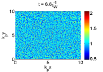
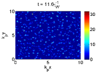
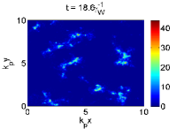
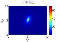
Figure 1: The beam density $n_{b}/n_{b0}$ in the beam cross-section at different moments of time. First, the beam breaks into a large number of non-stationary filaments in which fluctuations of the beam density are of the order of $n_{b0}$. Non-stationary filaments eventually coalesce into one quasistationary filament.

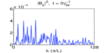
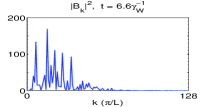
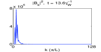
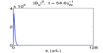
Figure 2: Evolution of the magnetic energy spectrum of perturbations. Growth of short-wave perturbations is suppressed due while long-wave perturbation grow until the system reaches equilibrium.

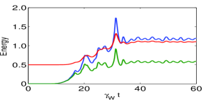
Figure 3: The evolution of the transverse kinetic energy of beam particles(blue), the magnetic energy (green), and the energy of plasma particles (red). The saturation level are of Non-zero initial value of the plasma energy is determined by the energy in the return current. The energy is measured in units $NT_{*}$, where $N$ is the number particles in the beam and $T_{*}=mc^{2}n_{b0}/n_{p}$.

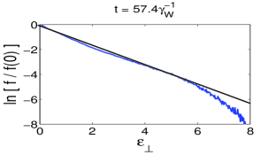
Figure 4: The beam particle distribution $\ln[f(\varepsilon_{\bot})/f(0)]$ over transverse kinetic energy $\varepsilon_{\bot}$ (measured in units $T_{*}$). The transverse temperature extracted from this dependence $T\approx 1.2T_{*}$.

When perturbations are small, the magnetic field energy grows exponentially with the growth rate of order $\gamma_{\mathrm{WI}}$ given by

$$\gamma_{\mathrm{WI}}(k_{\perp})=\omega_{p}\sqrt{\frac{n_{b}}{\gamma_{b}n_{p}}\frac{\beta_{z}^{2}k_{\perp}^{2}}{k_{\perp}^{2}+k_{p}^{2}}}.$$ (6)

where $\beta_{z}=v_{bz}/c$ and $\vec{k}_{\perp}$ is the transverse component of the wavevector. Although all modes with $k_{\perp}>>k_{p}$ grow simultaneously (with the rate $\gamma_{\mathrm{W}}=\gamma_{\mathrm{WI}}(k_{\perp}\rightarrow\infty)$), wavebreaking occurs first in short-wave modes and then in long-wave modes. Subsequent formation of multistream flow in the transverse beam motion effectively increases the transverse temperature of the beam particles. The thermal motion, in turn, suppresses growth of small-scale perturbations while large scale perturbations continue to grow. The dynamics of this complex process is illustrated in Fig. 2 where the evolution of the magnetic energy spectrum of perturbations is presented. The evolution of the transverse kinetic energy of beam particles and the magnetic energy is given in Fig. 3. In the course of multiple merging, non-stationary filaments become bigger and the distance between them increases. Eventually, they coalesce in one quasistationary filament (in our example, it happens at $t\sim 31\gamma_{W}^{-1}$). Often, this filament has elliptical form and slow rotation is observed. Particles in the filament perform complicated oscillatory motion along nonclosed trajectories. Nevertheless, our simulations show that the distribution function of the trapped particles over the transverse kinetic energy is approximately Maxwellian, see Fig. 4. Apparently, Maxwellization is caused by multi-generation merging of filaments.

Note that due to wavebreaking, fluctuations of the beam density become significant (of the order of $n_{b0}$) almost from the very beginning. As seen from Fig. 1, the density in the quasistationary filament exceeds tens times the initial level of the density. Although it is not noticeable in the figure, there is a big fraction of beam particles (in our case about $30\%$) outside of the filament in the large area where the final beam density is small, $n_{b}<n_{b0}$. These particles get dispersed in the process of multiple filament merging, and gain sufficient transverse temperature forming stable (against further development of Weibel instability) background .

III Estimates of the quasistationary filament parameters.

Characteristics of the quasistationary filament can be estimated by the following way. Making a rough assumption that all particles from $L\times L$ area are gathered in small area of the radius of the order of skin-depth length $\delta_{p}=k_{p}^{-1}$, one can estimate the beam density there as $n_{b}\sim n_{b0}\ast k_{p}^{2}L^{2}$ and the magnetic field as $B\sim 4\pi en_{b}/k_{p}$, so that $B^{2}\sim 4\pi mc^{2}n_{b}^{2}/n_{p}\sim 4\pi mc^{2}(n_{b0}^{2}/n_{p})k_{p}^{2}L^{2}$. Equating the transverse thermal pressure in the filament to the pressure of the magnetic field, $n_{b}T_{\perp}\sim B^{2}/8\pi$, one can estimate the transverse temperature in the beam filament

$$T_{\perp}\sim mc^{2}\frac{n_{b0}}{2n_{p}}k_{p}^{2}L^{2}\sim 2\pi mc^{2}\frac{I_{b}}{I_{A0}},$$ (7)

where $I_{A0}\equiv\beta mc^{3}/e$. This is a very rough estimate. More accurate formula (27) which takes into account the spatial distribution of beam particles in the filament gives considerably smaller numerical coefficient. The fraction of the longitudinal kinetic beam energy, $W_{||}=\gamma_{b}mc^{2}(n_{b0}L^{2})$, transferred to the transverse beam motion is given by

$$\frac{n_{b}(\pi k_{p}^{-2})T_{\perp}}{W_{||}}\sim(k_{p}L)^{2}\left(\frac{\gamma_{W}}{\omega_{p}}\right)^{2},$$ (8)

The energy transferred to the magnetic field and to the plasma is of the same order. Since the beam density $n_{b}$ in our consideration is always less than $n_{p}$, filaments of the radius $c/\omega_{p}$ carry sub-Alfvenic currents, $en_{b}c\beta_{z}\pi c^{2}/\omega_{p}^{2}<<\beta_{z}mc^{3}/e$.

IV Similarity and conservation laws for the beam filamentation dynamics in the limit of low density

When $n_{b}<<n_{p}$ during entire beam evolution and $\vec{V}_{b}\approx(0,0,-c)$, for analytical tractability we introduce further simplification in our hybrid model. To the first order in the small parameter $n_{b}/n_{p}$, the beam dynamics is governed by the equations:

$$k_{p}^{-2}\Delta\psi=\psi-(n_{b}/n_{p})mc^{2}/e,$$ (9)

$$m\gamma_{b}\frac{d\vec{v}_{j\perp}}{dt}=e\nabla_{\perp}\psi,$$ (10)

From these equations one can find that the evolution of the low density beam beam obeys a similarity law: it remains the same when space coordinates, time, the beam density and vector potential rescale as

$$\vec{r}_{\perp}\propto\lambda_{p},$$ (11)

$$t^{-1}\propto\omega_{p}\sqrt{n_{b0}/\gamma_{b}n_{p}}\sim\gamma_{W},$$ (12)

$$\vec{v}_{\perp}\propto c\sqrt{n_{b0}/\gamma_{b}n_{p}}\sim c(\gamma_{W}/\omega_{p}),$$ (13)

$$n_{b}\propto n_{b0},$$ (14)

$$\psi\propto(n_{b0}/n_{p})mc^{2}/e,$$ (15)

$$\frac{\gamma_{b}mv_{\perp}^{2}}{2}\propto mc^{2}n_{b}/n_{p}.$$ (16)

In particular, it means that at small beam densities it is enough to study beam propagation only at the one level of the initial density. The propagation at other levels can be found by rescaling the simulation results according to Eqs. (11)-(15). As seen from Eqs. (12), (13), (15) and (16), big beam relativistic factors $\gamma_{b}$ slow down the beam filamentation not changing magnetic fields created by filaments and transverse kinetic energy of beam particles.

It follows from the conservation of longitudinal momentum that for ultrarelativistic beam $\gamma_{b}mc^{2}\approx\gamma_{b0}mc^{2}+m\gamma_{b0}mv_{\perp}^{2}/2-e(\psi-\psi_{*})$, where $\psi_{*}$ is the initial value of the magnetic potential. The energy conservation law  Karmakar_ can be now transform to the form

$$W_{\perp}=\frac{1}{2}\int n_{b}m\gamma_{b}v_{\perp}^{2}dS-\frac{1}{2}\int en_{b}\psi dS=const.$$ (17)

This formula can be also derived directly from Eqs. (9) and (10). The potential energy is given by the second term in the right-hand side of Eq. (17); it includes the energy of the magnetic field and the plasma motion:

$$\frac{1}{2}\int en_{b}\psi dS=\frac{1}{2}\int B^{2}dS+\frac{1}{8\pi}\int n_{p}mv^{2}dS,$$ (18)

where $\vec{B}=\nabla\psi$ and $v=e\psi/mc$. The coefficient $1/2$ in front of the potential term reflects the fact that each particle is counted twice in the integral (17) so that the total energy of the one particle (which in general varies with time!) is

$$\epsilon_{tot}=\frac{\gamma_{b}mv_{\perp}^{2}}{2}-e\psi.$$ (19)

The magnetic potential forms a potential wells for particles, $U=-e\psi$; these wells merge with each other when corresponding filaments merge.

The other obvious integral on the motion of the system (9)-(10) is the conservation of the total number of the macroparticles:

$$N=\int n_{b}dS=const.$$ (20)

Note that for the beam with initially negligible transverse velocity spread homogeneously distributed over the area $L\times L$, the magnetic potential $\psi=(n_{b}/n_{p})mc^{2}/e$ and the total energy and number of particles are given by formulas,

$$W_{\perp}=-\frac{1}{2}Ne\psi_{*}=-\frac{1}{2}NT_{*},\quad N=n_{b0}L^{2},$$ (21)

where $e\psi_{*}=T_{*}=(n_{b0}/{n_{p}})mc^{2}$.

It is instructive to note that, in the framework of Eqs.  (9) and (10), the magnetic potential can be presented as a sum of potentials created by each beam particle,

$$\psi(\vec{r},t)=\frac{mc^{2}}{2\pi en_{p}}\int K_{0}(k_{p}|\vec{r}-\vec{r^{\prime}}|)n_{b}(\vec{r}^{\prime},t)d\vec{r}^{\prime}.$$ (22)

Thus, the interaction between particles in the low density beam is a pairwise Coulomb attraction screened by Bessel function at distances larger than the skin-depth $k_{p}^{-1}$, and the potential energy of beam particles can be presented as a sum of potential energies of all particle pairs.

V Structure of filaments

Figure 5 shows vertical and horizontal density cross-sections of the beam corresponding to the density distribution in the quasistationary filament in Fig. 1. As can be seen from this figure the filament pinched to the radius even smaller than the skin depth $\delta_{p}=k_{p}^{-1}$. For such radius the plasma screening of the magnetic field does not occur. Therefore, the magnetic pinching force is balanced by the pressure gradient $\nabla p=j\times B$ and $\nabla\times B=4\pi j/c$. This equilibrium correspond to the Bennett pinch DavBook

$$n_{b}=\frac{8/(k_{p}r_{B})^{2}}{(1+(r/r_{B})^{2})^{2}}\frac{T}{mc^{2}}n_{p},$$ (23)

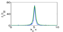
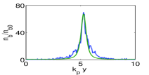
Figure 5: Crosssections of the filament density (blue) in $x$ and $y$ directions at the moment $t\approx 54\gamma_{W}^{-1}$. Green lines correspond to Bennett pinch with the radius $r_{B}=0.4k_{p}^{-1}$. The temperature of the filament is taken from simulations, $T=1.35mc^{2}n_{b0}/np$.

For the Bennett pinch the self-magnetic field outside of the filament is decreasing with radius $B=4\pi I/cr$ and magnetic potential $\psi$ decreases as $-4\pi(I/c)\ln r$. Therefore according to the Boltzmann relationship the density $n_{b\ast}\exp(e\psi/T)$ decreases as power law of radius. Due to plasma screening of the magnetic field, the magnetic field and variation of the magnetic flux vanishes at $r>>\delta_{p}$. Therefore density does not approach zero at large radius but tends to a finite value. This means that a low density halo forms outside filament. Detailed analysis shows that the total number density of particles in the halo is comparable to the total number density in the filament. See detail calculation in Appendix. Difference between Bennett distribution and modified Bennett distribution is illustrated in Fig. 6.

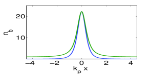
Figure 6: The beam particle density in Bennett pinch (red) and modified Bennett pinch (blue), $k_{p}r_{B}=0.6$.

The energy distribution of beam particles in the phase space space ($\varepsilon_{\perp},U$) obtained from our simulations is shown in Fig. 7. (For sake of convenience, the potential energy here is defined as $U=-e\psi+e\psi_{max}$.) One can see from this figure that the distribution function depends approximately only on the total particle energy $\varepsilon_{tot}=\varepsilon_{\perp}+U$. Such dependence is a simple consequence of the phase mixing of particles moving in the quasistationary potential well along trajectories with close total energies.

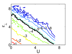
Figure 7: Contour lines of the beam particle distribution $\ln[f/f(0)]$ in the space formed by the transverse kinetic energy $\varepsilon_{\perp}=\gamma_{b}mv_{\perp}^{2}/2$ and potential energy $U=-e\psi+e\psi_{max}$ (measured in units $T_{*}=mc^{2}n_{b0}/n_{p}$). The variable $U$ changes from zero (in the center of the filament, where $e\psi=e\psi_{max}\approx 7.6mc^{2}n_{b0}/n_{p}$) to the value $7.3mc^{2}n_{b0}/n_{p}$ outside of the filament (where $e\psi=e\psi_{min}\approx 0.25mc^{2}n_{b0}/n_{p}$). Separatrix (black line) divides the phase space into two regions: the first region (in the shape of triangle) corresponds to particles trapped in the filament and the second one to untrapped particles. The point $\varepsilon_{\perp}=0$, $U=0$ corresponds to the cold particles at the center of the filament.

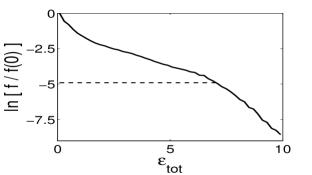
Figure 8: The beam particle distribution $\ln[f/f(0)]$ as a function of $\varepsilon_{tot}$ (measured in units $T_{*}$). Dashed line corresponds to the distribution function when energy exchange between electrons is absent.

The electron distribution as a function of $\varepsilon_{tot}$ is shown in Fig. 8. Note that if there is no energy exchanged between electrons, the beam particle distribution $f$ over total energy $\varepsilon_{tot}$ trapped in a potential well is constant  Gurevich . Because of the many events leading to the energy exchange during filament merger the energy electron distribution function is close to a Maxwellian (for ideal Maxwellian distribution function, $\ln[f/f(0)]$ should correspond to the straight line). However, there is significant departures from a Maxwellian for low and high total energy (deeply trapped and untrapped electrons). This because these electrons do not undergo many energy transfer with other electrons during filament merger. Low energy electrons are confined to the center of the filament and do not experience the time dependent magnetic field and inductive electric field during filament merger. Similarly untrapped electrons do not participate in energy transfer. Therefore, tail of the EEDF is strongly depleted at $\varepsilon_{tot}>\psi_{\max}-\psi_{\min}$ .

VI Energy transfer from the beam longitudinal kinetic energy to the beam transverse kinetic energy self magnetic field and plasma electrons

From two conservation laws, conservation of the number of particles and the energy conservation law, one can find the parameters $T$ and $r_{B}$ of the modified Bennett pinch and then the energy transfer from the beam longitudinal kinetic energy to the beam transverse kinetic energy, magnetic field and plasma electrons can be calculated.

Using the Boltzmann distribution of the density in quasistationary state, the conservation of the number of particles gives

$$n_{b\ast}\int\!\exp(e\psi/T)\,dS=N,$$ (24)

where $N=n_{b0}L^{2}$. For Maxwellian distribution function, the energy conservation law (17) with the initial constant (21) can be transformed to

$$TN=\frac{1}{2}n_{b\ast}\int\exp(e\psi/T)e(\psi-\psi_{*})dS,$$ (25)

where $\psi_{*}$ is the initial value of the magnetic potential. The term in the left-hand side corresponds to the transverse kinetic energy of the beam particles, and the term in the right-hand side corresponds to the increase in the effective potential energy. This increase is the same as the increase in the energy of the transverse motion (that is, $<\delta\psi>=T$). Thus, the energy drawn from the longitudinal motion of the beam during its evolution is:

$$<\Delta(\gamma_{b}mc^{2})_{||}>\approx-{2T},$$ (26)

After substituting the magnetic potential from Eq. (47) into Eqs. (24) and (25) and performing integrations, one can find the following asymptotic formula

$${T}=\frac{k_{p}^{2}L^{2}}{1+W(\alpha_{0}{k_{p}^{2}L^{2}})}\frac{T_{*}}{8\pi}=\frac{mc^{2}/2}{1+W(\alpha_{0}{k_{p}^{2}L^{2}})}\frac{I_{b}}{I_{A0}},$$ (27)

where $W(x)$ is the product logarithm (or Lambert W-function defined by the equation $W\exp(W)=x$), $\alpha_{0}=\exp(2\gamma_{E}-2)/4\pi=0.0341...$ and $\gamma_{E}=0.5772...$ is the Euler constant, $T_{*}=mc^{2}n_{b0}/n_{p}$ and $I_{b}/I_{A0}=en_{b0}cL^{2}/(mc^{3}/e)$. For $k_{p}L=10$, Eq. (27) gives $T\approx 1.7T_{*}$while simulations show that the transverse electron energy averaged over all beam particles is $30\%$ less: $<\varepsilon_{\perp}>=T\approx 1.2T_{*}$. The temperature is higher in the filament $T\approx 1.4T_{*}$ and lower outside of it. Difference between theoretical value of $T$ and that obtained from simulations is due to incomplete Maxwellization of the beam electron distribution function.

Since the product logarithm $W(x)\sim\ln(x/lnx)$ , one can conclude from Eq. (27) that the transverse temperature of the low-density beam slowly decreases as the beam cros-ssection aria increases (while the beam current is kept constant, $I_{b}=const$).

At large beam cross-section, the energy transfered from the beam longitudinal motion to the beam transverse motion, the magnetic field and the plasma motion is divided in the following way:

$$\frac{n_{b0}<\varepsilon_{\perp}>}{2n_{b0}T}=\frac{1}{2},$$ (28)

$$\frac{<B^{2}/8\pi>}{2n_{b0}T}\approx\frac{-\ln r_{B}+1.3r_{B}-0.88}{1+W(\alpha_{0}{k_{p}^{2}L^{2}})},$$ (29)

$$\frac{<n_{p}\Delta\varepsilon_{p}>}{2n_{b0}T}\approx\frac{1}{2}-\frac{-\ln r_{B}+1.3r_{B}-0.88}{1+W(\alpha_{0}{k_{p}^{2}L^{2}})}.$$ (30)

For $k_{p}L=10$, Eq. (52) gives $r_{B}\approx 0.4$ and Eq. (29) gives ${<B^{2}/8\pi>}/{2n_{b0}T}\approx 0.26$, and Eq. (30) gives ${<n_{p}\Delta\varepsilon_{p}>}/{2n_{b0}T}\approx 0.24$. One can find from Fig. 3 that the saturation level of the transverse kinetic energy of the beam ($1.2NT_{*}$) is two times higher than the saturation level of the magnetic energy ($0.6NT_{*}$). It is also two times higher than the saturation level of the plasma energy without initial energy ($0.6NT_{*}$). This observation is consistent with theoretical prediction.

VII Conclusion

We have considered the filamentation process of an electron beam with small density and large radius propagating through the dense plasma. We have found that the beam dynamics obeys simple similarity laws which simplify the beam description. During the formation of filaments and their merging the total transverse energy of the transverse motion of the beam particles is conserved. The effective transverse potential energy is comprised mostly of the energy of the magnetic field and the plasma motion and can be presented as a sum of pairwise interaction energies between beam particles.

Our particle-in-cell simulations have shown that all filaments eventually coalesce into one pinched beam although a significant fraction of the particles remains untrapped and scattered outside of this pinch. The electron beam distribution over the transverse kinetic energy is close to the Maxwellian one for the bulk of electrons. We have developed an analytical model and found the distribution of the particles in the modified Bennett pinch and in the low-density halo around it. In particular, we have found that the radius of the Bennett pinch modified by the return plasma current is always less or of the order of the plasma skin depth. For a given beam transverse size, we have calculated the energy transfer from the beam longitudinal motion to the transverse kinetic energy of the beam, the self-magnetic field and the plasma motion. It has turned out that the final transverse beam temperature is proportional to the beam current and slowly decreases with the beam radius. The results obtained from the model agree well with those obtained from particle-in-cell simulations.

Note that although our consideration is limited to initially cold beams, the calculations can be performed in a straightforward manner for the arbitrary case.

VIII
Appendix I. Detailed characteristics of modified Bennett pinch

In this section we describe the structure of an isolated filament similar to one shown in Fig. 1. We assume that all particles have Maxwellian distribution over velocities, i.e. the system is in a thermodynamic equilibrium. Hence, the density of particles is expected to be distributed in the effective potential $\psi$ according to Boltzmann law:

$$n_{b}=n_{b\ast}\exp(e\psi/T),$$ (31)

where $n_{b\ast}$ is some constant and $T$ is the transverse temperature (equal to the average transverse energy of a beam particle $T=<m\gamma_{b}v_{\perp}^{2}/2>$).

Substitution of Eq. (31) into Eq. (9) gives closed equation for the vector potential

$$k_{p}^{-2}\Delta\psi=\psi-\frac{mc^{2}}{en_{p}}n_{b*}\exp\Big{(}\frac{e\psi}{T}\Big{)}.$$ (32)

Since the magnetic filed is small far from the filament, the magnetic potential should be constant at large distances from the filament. Under this condition, equation (32) determines the function $\psi(x,y)$ at each value of the parameter $n_{b*}$. In one dimensional case when all quantities depend on one transverse coordinate $x$, one can solve Eq. (32) analytically and find the potential and density distribution in an isolated filament, see Appendix II.

In two dimensional case when particles are gathered from large area $L\times L$ ( much bigger than the aria occupied by the filament), the fully thermalized filament is axially symmetric and therefore Eq. (32) can be transform to

$$\frac{1}{k_{p}^{2}r}\frac{d}{dr}r\frac{d}{dr}\Big{(}\frac{e\psi}{T}\Big{)}=\frac{e\psi}{T}-\frac{1}{k_{p}^{2}r_{D}^{2}}\exp\Big{(}\frac{e\psi}{T}-\frac{e\psi_{0}}{T}\Big{)}.$$ (33)

where $r_{D}=[T/4\pi e^{2}n_{b}(0)]^{1/2}$ is the Debye radius corresponding to the beam density at the filament center, $n_{b}(0)=n_{b*}\exp(e\psi_{0}/T)$, and $\psi_{0}=\psi(0)$. This equation can be solved numerically by the shooting method: at given value of the parameter $k_{p}r_{D}$, we find such $e\psi_{0}/{T}$ at which the magnetic potential $\psi$ is a monotonically decreasing function of $r$ with asymptote $\psi\rightarrow\psi_{\infty}$ and $d\psi/dr\rightarrow 0$ at $r\rightarrow\infty$.

It turns out that the solution with these properties exists only when $k_{p}r_{D}<1$. Indeed, at the point $r=0$ where the magnetic potential reaches maximum, we have $\psi=\psi_{0}$, $d\psi/dr=0$, and $d^{2}\psi/dr^{2}<0$. Therefore, the right-hand side of Eq. (33) should be negative at this point, that is,

$$\frac{e\psi_{0}}{T}<\frac{1}{k_{p}^{2}r_{D}^{2}}.$$ (34)

On the other hand, the expression in the right-hand side of Eq. (33) should be equal to zero at large $r$. Therefore,

$$\frac{e\psi_{\infty}}{T}=\frac{1}{k_{p}^{2}r_{D}^{2}}\exp\Big{(}\frac{e\psi_{\infty}}{T}-\frac{e\psi_{0}}{T}\Big{)}>\frac{e\psi_{0}}{T}\exp\Big{(}\frac{e\psi_{\infty}}{T}-\frac{e\psi_{0}}{T}\Big{)}.$$ (35)

After simple manipulations, we find that $\psi_{\infty}$ and $\psi_{0}$ satisfy to the following condition,

$$F\Big{(}-\frac{e\psi_{\infty}}{T}\Big{)}<F\Big{(}-\frac{e\psi_{0}}{T}\Big{)}\quad at\quad\frac{e\psi_{\infty}}{T}<\frac{e\psi_{0}}{T},$$ (36)

where $F(x)\equiv-x\exp(-x)$. Since this function grows only at $x>1$, $F^{\prime}(x)=(x-1)\exp(-x)$, the condition (36) imposes restriction on the maximum value of the magnetic potential, $e\psi_{0}/T>1$. It means that filament-like solutions exist only when $1/{k_{p}^{2}r_{D}^{2}}>e\psi_{0}/T>1$, that is, only when $k_{p}r_{D}<1$. Note that the trivial solution of Eq. (33) $e\psi/T=const=1/k_{p}^{2}r_{D}^{2}$ exists at all values of $k_{p}r_{D}$. However, when $k_{p}r_{D}\geq 1$, there are no other solutions except the trivial one: the Weibel instability is suppressed by the thermal motion of particles, and the beam remains homogeneous with $n_{b}=const$.

Figure 9 shows the magnetic potential as a function of $r$ at different Debye radii. Note that $e\psi_{0}/T=1$ at $k_{p}r_{D}=1$, $e\psi_{0}/T\approx 4.3$ at $k_{p}r_{D}=0.23$, and $e\psi_{/}T\approx 11.8$ at $k_{p}r_{D}=0.022$. Analysis of the monotonic solution $\psi(r)$ at even smaller Debye radii suggests that the magnetic potential at the filament center grows approximately as

$$e\psi_{0}/T\approx-4\ln k_{p}r_{D}-3.7,$$ (37)

when $k_{p}r_{D}\rightarrow 0$. Therefore, near the filament center (at the distances $r\sim r_{D}$) the plasma return current is much smaller than the beam current ($e\psi_{0}/T<<1/k_{p}^{2}r_{D}^{2}$). On the other hand, because the beam current decreases faster than the plasma return current, the latter becomes dominant at distances $r>>r_{D}$. At even larger distances $r\gtrsim k_{p}^{-1}$, these currents reaching the minimum value become equal to each other.

This currents’ behavior allows us to find the approximate analytical solution of Eq. (33) at small $k_{p}r_{D}$.

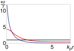
Figure 9: The magnetic potential at different values of the Debye radius: $k_{p}r_{D}=1$ (black), $k_{p}r_{D}=0.23$ (red), and $k_{p}r_{D}=0.022$ (blue).

Omitting the first term in the right-hand side of Eq. (32) near the filament center, we obtain

$$\frac{1}{k_{p}^{2}r}\frac{d}{dr}r\Big{(}\frac{e\psi}{T}\Big{)}=-\frac{1}{k_{p}^{2}r_{D}^{2}}\exp\Big{(}\frac{e\psi}{T}-\frac{e\psi_{0}}{T}\Big{)}.$$ (38)

This equation describes the Bennett distribution of beam particles with uniform transverse beam temperature DavBook :

$$e\psi/T=e\psi_{0}/T-2\ln[(1+(r/r_{B})^{2}],$$ (39)

$$n_{b}=\frac{8/(k_{p}r_{B})^{2}}{(1+(r/r_{B})^{2})^{2}}\frac{T}{mc^{2}}n_{p},$$ (40)

where $r_{B}=2\sqrt{2}r_{D}$ is the radius of the Bennett pinch The Bennett distribution is accurate at small distances from the filament center, $r\sim r_{B}$, where magnetic screening is negligible.

In the range of distances $r_{B}\lesssim r\lesssim k_{p}^{-1}$, where the plasma return current is dominant, one can omit the second term in the right-hand side of Eq. (32),

$$\frac{1}{k_{p}^{2}r}\frac{d}{dr}r\frac{d}{dr}\Big{(}\frac{e\psi}{T}\Big{)}=\frac{e\psi}{T},\quad\frac{e\psi}{T}=aK_{0}(k_{p}r),$$ (41)

where $a$ is some constant, and $K_{0}$ is the modified Bessel function of the second kind. Solutions (39) and (41) should match at distances, $r_{B}<<r<<k_{p}^{-1}$. The magnetic potential in the Bennett pinch has the following asymptotics at $r>>r_{B}$:

$$\frac{e\psi}{T}\approx\frac{e\psi_{0}}{T}+4\ln(k_{p}r_{B})-4\ln k_{p}r,$$ (42)

while the solution (41) at $r<<k_{p}^{-1}$ can be approximated by:

$$\frac{e\psi}{T}\approx a(-\gamma_{E}+\ln 2-\ln k_{p}r),$$ (43)

where $\gamma_{E}=0.5772...$ is the Euler constant. Comparison of (42) and (43) gives $a=4$ and the expression for the magnetic potential at the filament center,

$$\frac{e\psi_{0}}{T}=-4\ln(k_{p}r_{B})+4(-\gamma_{E}+\ln 2),$$ (44)

which, after substitution $r_{B}^{2}=8r_{D}^{2}$, reduces to the expression Eq. (37) found by the shooting method. Using Eq.(44), we find that the constant $n_{b*}$ in Boltzmann distribution at small $k_{p}r_{D}$ is given by

$$\frac{{n}_{b*}}{n_{p}}=\frac{T}{mc^{2}}\frac{\exp{(-e\psi_{0}/T)}}{k_{p}^{2}r_{D}^{2}}=\alpha_{1}{k_{p}^{2}r_{B}^{2}}\frac{T}{mc^{2}},$$ (45)

where $\alpha_{1}\equiv\exp(4\gamma_{E})/2\approx 5.0$. At large distances from the filament center where the beam and plasma currents become equal to each other, the magnetic potential $\psi_{\infty}$ is determined by the equation $e\psi_{\infty}/T=(mc^{2}/T)(n_{b*}/n_{p})\exp{(e\psi_{\infty}/T)}$ and equal to

$$\frac{e\psi_{\infty}}{T}=-W(-\alpha_{1}k_{p}^{2}r_{D}^{2})\approx\alpha_{1}k_{p}^{2}r_{D}^{2},$$ (46)

where $W(x)$ is the Lambert W-function. It is convenient to use the interpolation formulas for the magnetic potential and beam particles distribution which work at all distances and can be used even for moderately small parameter $k_{p}r_{B}$,

$$\frac{e\psi}{T}=4K_{0}[k_{p}(r^{2}+r_{B}^{2})^{1/2}]+\frac{e\psi_{\infty}}{T},$$ (47)

$$n_{b}=\frac{8/(k_{p}r_{B})^{2}}{(1+(r/r_{B})^{2})^{2}}\frac{T}{mc^{2}}n_{p}+n_{b\infty},$$ (48)

where $n_{b\infty}=(n_{p}T/{mc^{2}}){e\psi_{\infty}}/T$. These formulas describe the modified Bennett distribution of the beam particles in the presence of plasma return current.

We have found a general solution of Eq.(32) which depends on the transverse temperature of beam particles $T$, and the radius of the Bennett pinch $r_{B}$ (or $r_{D}$). For an arbitrary transverse beam dimension, these two parameters can be determined from two conservation laws. The procedure is straightforward when the solution of Eq.(32) is found numerically; the result for is presented in Fig. 5 by purple bullets. To find analytical formulas, we introduce dimensionless variables $\tilde{\psi}=e\psi/T$, $\tilde{n}=mc^{2}n_{b}/(Tn_{p})$, and dimensionless parameters $\tilde{T}=T/T_{*}$ (where $T_{*}=mc^{2}n_{b0}/n_{p}$), $\tilde{n}_{\infty}=mc^{2}n_{b\infty}/(Tn_{p})$, and $\tilde{\psi}_{0}=e\psi_{0}/T$. Substituting Eq. (48) into Eq. (24), we can evaluate the number of particles as

$$8\pi\tilde{T}+\tilde{n}_{b\infty}\tilde{T}k_{p}^{2}L^{2}=k_{p}^{2}L^{2},$$ (49)

The first term in the left-hand side of this equation is proportional to the number of the particle in the Bennett pinch and the second term is proportional to the number of particles outside of the pinch. To evaluate the potential energy at small $k_{p}r_{B}$, we use Eqs. (39) and (39) and transform Eq. (25) to

$$\tilde{T}k_{p}^{2}L^{2}-\frac{1}{2}\tilde{T}^{2}(8\pi\tilde{\psi}_{0}-16\pi)=-\frac{1}{2}k_{p}^{2}L^{2},$$ (50)

We can make further simplification, noting that $\tilde{T}>>1$ when $k_{p}L>>1$ and neglecting the term in the right-hand side of Eq.(50) proportional to the initial potential energy. Using Eq. (44) and formula $\tilde{n}_{b\infty}=\alpha_{1}k_{p}^{2}r_{B}^{2}$, we find the temperature and the radius

$${T}=\frac{k_{p}^{2}L^{2}}{1+W(\alpha_{0}{k_{p}^{2}L^{2}})}\frac{T_{*}}{8\pi},$$ (51)

$$k_{p}^{2}r_{B}^{2}=\frac{8\pi}{\alpha_{1}k_{p}^{2}L^{2}}W[\alpha_{0}(k_{p}L+A_{1})^{2}].$$ (52)

Surprisingly despite all approximations, formula (51) very closely reproduces the result of the numerical integration of Eq. (32), see Fig. 10 (left panel). To improve accuracy of the other formula, we introduce the adjustment parameter $A_{1}$ into Eq. (52), otherwise it is not accurate at moderately large $k_{p}L$. Comparison of the adjusted ($A_{1}=35$) and unadjusted ($A_{1}=0$) formulas with the result obtained by the shooting method is given on the right panel in this figure.

,

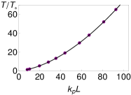
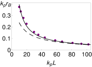
Figure 10: The parameters $T$ and $r_{B}$ of the modified Bennett pinch as a function of the transverse beam dimension $L$. The pinch is obtained from Eq. (32) by the shooting method (purple bullets) and analytically (black lines). The dashed black line corresponds to the analytical formula for the radius without adjustment.

Now we find several integral characteristics of the modified Bennett pinch. It is interesting to note that the total magnetic energy $W_{m}$ in this pinch is a finite quantity (in contrast to the regular Bennett pinch, where it diverges at large distances). Using Eq. (47) we calculate $\vec{B}=-\nabla\psi$ and then integrate $B^{2}/8\pi$ over the transverse area. The result can be expressed in special functions; with some adjustments, it is given at at small $k_{p}r_{B}$ by

$$W_{m}=\frac{T^{2}}{4\pi e^{2}}(-44.4+66k_{p}r_{B}-16\pi\ln k_{p}r_{B}).$$ (53)

The number of particles trapped in the modified Bennett pinch can be found by integrating Eq. (48) over the transverse area. Using Eq. (51) and making some adjustments, we find

$$N_{tr}=N\frac{1+0.83r_{B}}{1+W(\alpha_{0}k_{p}^{2}L^{2})}.$$ (54)

where $r_{B}$ should be calculated from Eq.(52). Obviously, the number of untrapped particles is given by

$$N_{untr}=N\frac{W(\alpha_{0}k_{p}^{2}L^{2})-0.83r_{B}}{1+W(\alpha_{0}k_{p}^{2}L^{2})}.$$ (55)

- (1) E. W. Weibel, Phys. Rev. Lett. 2, 83 (1959).
- (2) B. D. Fried, Phys. Fluids, 2, 337 (1959)
- (3) R. L. Morse and C. W. Nielson, Phys. Fluids 14, 830 (1971).
- (4) R. C. Davidson et al., Phys. Fluids 15, 317 (1972).
- (5) R. Lee and M. Lampe, Phys. Rev. Lett. 31, 1390 (1973).
- (6) M. V. Medvedev and A. Loeb, ApJ 526, 697 (1999).
- (7) M. V. Medvedev et al., ApJ 618, L75 (2005).
- (8) A. Gruzinov, ApJ 563, L15 (2001).
- (9) L. O. Silva et al., Phys. Plasmas 9, 2458 (2002).
- (10) M. Milosavljevic et al., ApJ 637, 765 (2006).
- (11) A. Spitkovsky, arXiv:0706.3126 (2007).
- (12) M. Tabak et al., Phys. Plasmas 1, 1626 (1994).
- (13) J. J. Honrubia and J. Meyer-ter-Vehn, Nucl. Fusion 46, L25 (2006).
- (14) S. Atzeni and J. Meyer-ter-Vehn, The Physics of Inertial Fusion (Oxford U. Press, New York, 2004), p. 409.
- (15) T. Taguchi et al., Phys. Rev. Lett. 86, 5055 (2001).
- (16) L. O. Silva et al., Phys. Plasmas 10, 1979 (2003).
- (17) V. M. Malkin and N. J. Fisch, Phys. Rev. Lett. 89, 125004 (2002).
- (18) J. M. Hill et al., Phys. Plasmas 12, 082304 (2003).
- (19) O. Polomarov, A. Sefkow, I. Kaganovich, and G. Shvets, Phys. Plasmas 14, 043103 (2007).
- (20) M. Honda et al., Phys. Rev. Lett. 85, 2128 (2000).
- (21) L. O. Silva et al., Astrophys. J. 596, L121 (2003).
- (22) R. C. Davidson, Physics of nonneutral plasmas (Addison-Wesley, 1990), p. 122.
- (23) O. Polomarov, I. Kaganovich, and G. Shvets, Phys. Rev. Lett. 101, 175001 (2008).
- (24) Gennady Shvets, Oleg Polomarov, Vladimir Khudik, Carl Siemon and Igor Kaganovich, Phys. Plasmas 16, 056303 (2009).
- (25) B. I. Cohen, A. B. Langdon, D. W. Hewett, and R. J. Procassini, J. Comp. Phys. 81, 151 (1989).
- (26) LSP is a software product of ATK Mission Research, Albuquerque, NM 87110.
- (27) Ya. B. Fainberg, V. D. Shapiro, and V. I. Shevchenko, Sov. Phys. JETP 30, 528 (1970) [Zh. Eksp. Teor. Fiz. 57, 966 (1969)].
- (28) M. Lampe and P. Sprangle, Phys. Fluids 18, 475 (1975).
- (29) M. E. Dieckmann, B. Eliasson, P. K. Shukla, N. J. Sircombe, and R. O. Dendy, Plasma Phys. Control. Fusion 48, B303 (2006).
- (30) A. Bret et al., Phys. Rev. Lett. 94, 115002 (2005).
- (31) T. N. Kato, Phys. Plasmas 12, 080705 (2005).
- (32) D. A. Hammer and N. Rostoker, Phys. Fluids 13, 1831 (1970).
- (33) E. P. Lee, S. Yu, H. L. Buchanan, F. W. Chanbers, and M. N. Rosenbluth, Phys. Fluids 23, 2095 (1980).
- (34) I. D. Kaganovich, G. Shvets, E. Startsev, and R. C. Davidson, Phys. Plasmas 8, 4180 (2001).
- (35) A. V. Gurevich, Zh. Exp Teor. Fiz.53, 953 (1967).[English translation: Soviet Phys. JETP 26,953 (1968)].
- (36) O. Buneman, Proc. R. Soc. London, Ser. A 215, 346 (1952).
- (37) A. Karmakar,1 N. Kumar, G. Shvets, O. Polomarov, and A. Pukhov, Phys. Rev. Lett. 101, 255001 (2008).