The Elemental Shear Dynamo

Abstract

A quasi-linear theory is presented for how randomly forced, barotropic velocity fluctuations cause an exponentially-growing, large-scale (mean) magnetic dynamo in the presence of a uniform shear flow, $\boldsymbol{U}=Sx\boldsymbol{e}_{y}$. It is a “kinematic” theory for the growth of the mean magnetic energy from a small initial seed, neglecting the saturation effects of the Lorentz force. The quasi-linear approximation is most broadly justifiable by its correspondence with computational solutions of nonlinear magnetohydrodynamics, and it is rigorously derived in the limit of large resistivity, $\eta\rightarrow\infty$. Dynamo action occurs even without mean helicity in the forcing or flow, but random helicity variance is then essential. In a sufficiently large domain and with small wavenumber $k_{z}$ in the direction perpendicular to the mean shearing plane, a positive exponential growth rate $\gamma$ can occur for arbitrary values of $\eta$, the viscosity $\nu$, and the random-forcing correlation time $t_{f}$ and phase angle $\theta_{f}$ in the shearing plane. The value of $\gamma$ is independent of the domain size. The shear dynamo is “fast”, with finite $\gamma>0$ in the limit of $\eta\rightarrow 0$. Averaged over the random forcing ensemble, the ensemble-mean magnetic field grows more slowly, if at all, compared to the r.m.s. field (magnetic energy). In the limit of small Reynolds numbers ($\eta,\ \nu\rightarrow\infty$), the dynamo behavior is related to the well-known alpha–omega ansatz when the forcing is steady ($t_{f}\rightarrow\infty$) and to the “incoherent” alpha–omega ansatz when the forcing is purely fluctuating.

1 Introduction

This paper presents a theory that yields exponential growth of the horizontally-averaged magnetic field (i.e., a large-scale dynamo) in the presence of a time-mean horizontal shear flow and a randomly fluctuating, 3D, barotropic force (i.e., with spatial variations only within the mean shearing plane) in incompressible magnetohydrodynamics (MHD). This configuration provides perhaps the simplest paradigm for a dynamo without special assumptions about the domain geometry or forcing (e.g., without mean kinetic helicity). We call it the elemental shear dynamo (ESD). There is a long history of dynamo theory (Moffatt, 1978; Krause & Radler, 1980; Roberts & Soward, 1992; Brandenburg & Subramanian, 2005), but much of it is comprised of ad hoc closure ansatz (i.e., not derived from fundamental principles and devised for the intended behavior of the solutions) for how fluctuating velocity and magnetic fields act through the mean electromotive force curl to amplify the large-scale magnetic field. Here the horizontal-mean magnetic field equation is derived within the “quasi-linear” dynamical approximations of randomly forced linear shearing waves and flow-induced magnetic fluctuations.

In the standard ansatz (Moffatt, 1978) , the mean-field equation in dynamo theory has the functional form of

$$\partial_{t}\overline{\boldsymbol{B}}=\mathsfbi{L}\cdot\overline{\boldsymbol{B}}+\mathsfbi{D}:\nabla\overline{\boldsymbol{B}}+\dots\,,$$ (1)

where the over-bar indicates some suitably defined average; $\overline{\boldsymbol{B}}$ is the mean magnetic field; and $\mathsfbi{L}$ and $\mathsfbi{D}$ are second- and third-order tensor operators (often denoted by $\alpha$ and $\beta$) that express the statistical effects of the velocity field $\boldsymbol{v}$ through the curl of the mean electromotive force, $\overline{\nabla\times(\boldsymbol{v}\times\boldsymbol{B})}$. The dots encompass possible higher-order derivatives of $\overline{\boldsymbol{B}}$ (which would be relatively small if there were a spatial scale separation between the mean field and the fluctuations) and resistive diffusion. If $\boldsymbol{v}$ itself is steady in time, then (1) is an exact form for the electromotive effect, and the kinematic dynamo problem can be viewed as an eigenvalue problem for the exponential growth rate $\gamma$ given $\overline{\boldsymbol{v}}$; in this case, however, there will be no scale separation between $\overline{\boldsymbol{v}}$ and $\overline{\boldsymbol{B}}$, and $\gamma$ may not be positive. An important weakness in such an ansatz is the lack of justification for particular forms of $\mathsfbi{L}$ and $\mathsfbi{D}$ in time-dependent flows. We will see that the ESD theory provides a clear justification, and it mostly does not fit within the ansatz (1) because the tensors are time-integral operators except in particular limits (Sec. 5).

The ESD problem specifies a steady flow with uniform shear $S$, a small initial seed amplitude and vertical wavenumber $k_{z}$ for the mean magnetic field, and a particular horizontal wavenumber $\boldsymbol{k}_{\perp f}$ and correlation time $t_{f}$ for the random force. It defines an ensemble of random-force time series that each gives rise to a statistically stationary velocity field, and the induced dynamo behavior is assessed over long integration times with further ensemble averaging.

This paper takes a general parametric view of the ESD derivation and solutions. A parallel report utilizing a minimal proof-of-concept derivation for the treble limit of small kinetic and magnetic Reynolds numbers and weak mean shear is in Heinemann et al. (2011a); the relation between the two papers is described in Sec. 5.2. The experimental basis for developing the ESD theory is the 3D MHD simulations in Yousef et al. (2008a, b). They show a large-scale dynamo in a uniform shear flow with a random, small-scale force at intermediate kinetic and magnetic Reynolds numbers. Their dynamo growth rate is not affected by a background rotation, even Keplerian. Additionally, new 2⁺D simulations — a barotropic velocity with spatial variations only within the mean shearing plane $(x,y)$ and a magnetic field with $(x,y)$ variations plus a single wavenumber $k_{z}$ in the vertical direction $z$ perpendicular to the plane — also manifests a large-scale dynamo (Heinemann et al., 2011b). Furthermore, within this 2⁺D model, successive levels of truncation of Fourier modes in the shearing-plane wavenumber demonstrate that its dynamo behavior persists even into the quasi-linear situation for which the mean-field theory is derived here. Thus, the dynamo solutions of the ESD theory are a valid explanation for computational dynamo behavior well beyond the asymptotic limit of vanishing magnetic Reynolds number.

From general MHD for fluctuations in a shear flow (Sec. 2), a quasi-linear model is developed for shearing waves (Sec. 3) and for induced magnetic fluctuations and the horizontal-mean magnetic field evolution equation with dynamo solutions (Sec. 4). Analytic expressions for the dynamo growth rate $\gamma$ are derived in Sec. 5 for several parameter limits, and general parameter dependences are surveyed in Sec. 6. Section 7 summarizes the results and anticipates future generalizations and tests.

2 Governing Equations

The equations of incompressible MHD are the Navier-Stokes equation for velocity $\boldsymbol{v}$,

$$\partial_{t}\boldsymbol{v}+\boldsymbol{v}\cdot\nabla\boldsymbol{v}=-\,\frac{1}{\rho}\nabla p+\boldsymbol{B}\cdot\nabla\boldsymbol{B}+\nu\nabla^{2}\boldsymbol{v}+\boldsymbol{f}\,,$$ (2)

where $\boldsymbol{f}$ is a prescribed forcing function, density $\rho$ is constant, and pressure $p$ is determined by the constraint,

$$\nabla\cdot\boldsymbol{v}=0\,,$$ (3)

and the magnetic induction equation for $\boldsymbol{B}$ (in velocity units),

$$\partial_{t}\boldsymbol{B}+\boldsymbol{v}\cdot\nabla\boldsymbol{B}=\boldsymbol{B}\cdot\nabla\boldsymbol{v}+\eta\nabla^{2}\boldsymbol{B}\,,$$ (4)

with

$$\nabla\cdot\boldsymbol{B}=0\,.$$ (5)

An exact, conservative solution to the above equations is given by an unmagnetized, uniform shear flow of the form

$$\boldsymbol{v}=Sx\boldsymbol{e}_{y},\quad\boldsymbol{B}=0\,,$$ (6)

where the shear rate $S$ is a constant in space and time and $\boldsymbol{e}$ denotes a unit vector. To study the dynamics of fluctuations on top of the background shear flow (6), we rewrite the equations of motion in terms of the velocity fluctuations $\boldsymbol{u}$ defined through

$$\boldsymbol{v}=Sx\boldsymbol{e}_{y}+\boldsymbol{u}\,.$$ (7)

Assume that the volume average of $\boldsymbol{u}$ is zero. Substituting (7) into (2) and (4) yields

$$\mathcal{D}\boldsymbol{u}+\boldsymbol{u}\cdot\nabla\boldsymbol{u}+Su_{x}\boldsymbol{e}_{y}=-\nabla p+\boldsymbol{B}\cdot\nabla\boldsymbol{B}+\nu\nabla^{2}\boldsymbol{u}$$ (8)

and

$$\mathcal{D}\boldsymbol{B}+\boldsymbol{u}\cdot\nabla\boldsymbol{B}=\boldsymbol{B}\cdot\nabla\boldsymbol{u}+SB_{x}\boldsymbol{e}_{y}+\eta\nabla^{2}\boldsymbol{B}\,,$$ (9)

where

$$\mathcal{D}=\partial_{t}+Sx\partial_{y}\,.$$ (10)

The only explicit coordinate dependence in (8) and (9) arises through the differential operator (10), which contains the cross-stream coordinate $x$. This means that we can trade the explicit $x$-dependence for an explicit time dependence by a transformation to a shearing-coordinate frame, defined by

$$x^{\prime}=x,\quad y^{\prime}=y-Stx,\quad z^{\prime}=z,\quad t^{\prime}=t\,.$$ (11)

Partial derivatives with respect to primed and unprimed coordinates are related by

$$\partial_{x^{\prime}}=\partial_{x}+St\partial_{y}\,,\quad\partial_{y^{\prime}}=\partial_{y}\,,\quad\partial_{z^{\prime}}=\partial_{z}\,,\quad\partial_{t^{\prime}}=\partial_{t}+Sx\partial_{y}=\mathcal{D}\,,$$ (12)

which shows that the explicit spatial dependence is indeed eliminated in the shearing frame. Therefore in shearing coordinates there are spatially periodic solutions, in particular a Fourier amplitude and phase factor, expressed alternatively as

$$\chi(x,y,z,t) =\mathrm{Re}\left\{\,\hat{\chi}(t)\exp\Bigl{[}\mathrm{i}k_{x}(t)x+\mathrm{i}k_{y}y+\mathrm{i}k_{z}z\Bigr{]}\,\right\}$$

$$=\mathrm{Re}\left\{\,\hat{\chi}(t^{\prime})\exp\Bigl{[}\mathrm{i}k_{x0}x^{\prime}+\mathrm{i}k_{y}y^{\prime}+\mathrm{i}k_{z}z^{\prime}\Bigr{]}\,\right\}\,,$$ (13)

where the transverse wavenumber $k_{y}$ and the spanwise wave number $k_{z}$ are constant in both coordinate frames, but the streamwise wavenumber $k_{x}$ varies in time according to $k_{x}(t)=k_{x0}-Sk_{y}t$. For an observer in the unprimed (“laboratory”) coordinate system, a disturbance that varies along the streamwise direction stretches out as a result of being differentially advected by the background shear flow; for an observer in the shearing frame the Fourier phase has fixed wavenumbers $(k_{x0},k_{y0},k_{z})$.

3 Dynamics

3.1 Simplifications

Guided by the experimental demonstrations of the shear dynamo (Yousef et al., 2008a, b; Heinemann et al., 2011b), we make the following simplifying assumptions:

1. The magnetic field strength is sufficiently small so that there is no back reaction onto the flow. In this so-called kinematic regime, we drop the Lorentz force.

2. The 3D forcing is restricted to two-dimensional spatial variations in the horizontal $(x,y)$ plane (i.e., barotropic flow with $\partial_{z}\boldsymbol{u}=\partial_{z}p=0$). (With this assumption it makes no difference whether the system is rotating around the $\boldsymbol{e}_{z}$ axis or has a stable density stratification aligned with $\boldsymbol{e}_{z}$. For these dynamical influences to matter, $\boldsymbol{u}$ has to have 3D spatial dependence.) In this case the dynamics reduce to forced 2D advection-diffusion equations for the vertical velocity, $u_{z}$, and the vertical vorticity, $\omega_{z}=\boldsymbol{e}_{z}\cdot(\nabla_{\perp}\times\boldsymbol{u}_{\perp})$; viz.,

   $$\mathcal{D}u_{z}+\boldsymbol{u}_{\perp}\cdot\nabla_{\perp}u_{z} =\nu\nabla_{\perp}^{2}u_{z}+f_{z}$$

   $$\mathcal{D}\omega_{z}+\boldsymbol{u}_{\perp}\cdot\nabla_{\perp}\omega_{z} =\nu\nabla_{\perp}^{2}\omega_{z}+\boldsymbol{e}_{z}\cdot(\nabla_{\perp}\times\boldsymbol{f}_{\perp})\,.$$ (14)

   We use a notation for a horizontal vector as

   $$\boldsymbol{a}_{\perp}=a_{x}\boldsymbol{e}_{x}+a_{y}\boldsymbol{e}_{y}\,.$$ (15)

   Because $\boldsymbol{u}$ has no $z$ dependence, the non-divergence condition reduces to $\nabla_{\perp}\cdot\boldsymbol{u}_{\perp}=0$, and we introduce a streamfunction $\Phi$ for the horizontal velocity and its associated vertical vorticity:

   $$\boldsymbol{u}_{\perp}=\boldsymbol{e}_{z}\times\nabla_{\perp}\Phi\,,\qquad\omega_{z}=\nabla_{\perp}^{2}\Phi\,.$$ (16)

3. Fluctuation advection is neglected in (14), so the vertical momentum and vorticity balances are linear.

   $$\mathcal{D}u_{z} =\nu\nabla^{2}u_{z}+f_{z}$$

   $$\mathcal{D}\omega_{z} =\nu\nabla_{\perp}^{2}\omega_{z}+\boldsymbol{e}_{z}\cdot(\nabla_{\perp}\times\boldsymbol{f}_{\perp})\,.$$ (17)

3.2 Conservative Shearing Waves

For linearized conservative dynamics ($\boldsymbol{f}=0$, $\nu=0$), (17) is

$$\mathcal{D}u_{z}=\mathcal{D}\omega_{z}=0\,.$$ (18)

The Fourier mode solutions are

$$u_{z} =\mathrm{Re}\left\{\,\hat{u}_{z0}\,e^{\mathrm{i}\phi}\,\right\}$$

$$\omega_{z} =\mathrm{Re}\left\{\,\hat{\omega}_{z0}e^{\mathrm{i}\phi}\,\right\}\,,$$ (19)

with a phase function that can be alternatively expressed in shearing or laboratory coordinates as

$$\phi=k_{x}^{\prime}x^{\prime}+\mathrm{i}k_{y}^{\prime}y^{\prime}=k_{x}(t)x+\mathrm{i}k_{y0}y\,.$$ (20)

The constants $k_{x}^{\prime}=k_{x0}$, $k_{y}^{\prime}=k_{y0}$, $\hat{u}_{z0}$, and $\hat{\omega}_{z0}$ are set by the initial conditions, and a tilting $x$-wavenumber is defined by $k_{x}(t)=k_{x0}-Sk_{y0}t$. From (16) the associated horizontal velocity is

$$\boldsymbol{u}_{\perp}=\frac{-\,\boldsymbol{e}_{z}\times\boldsymbol{k}_{\perp}(t)}{k_{\perp}^{2}(t)}\,\mathrm{Re}\left\{\,\mathrm{i}\,\hat{\mathcal{\omega}}_{z0}e^{\mathrm{i}\phi}\,\right\}\,,$$ (21)

where $k_{\perp}^{2}=k_{x}^{2}+k_{y0}^{2}$. Notice that $\boldsymbol{u}_{\perp}(t)$ grows when $k_{x}(t)/k_{y0}>0$ by extracting kinetic energy from the mean shear (an up-shear phase tilt), and it decays when $k_{x}(t)/k_{y0}<0$ (down-shear). As $t\rightarrow\infty$, $\boldsymbol{u}_{\perp}\rightarrow 0$ for any $\boldsymbol{k}_{0}$. This shearing wave behavior is sometimes called the Orr effect.

3.3 Single-Mode Forcing

In a quasi-linear theory the random fluctuations can be Fourier decomposed into horizontal wavenumbers, and the resulting velocity and magnetic fields summed over wavenumber. It suffices to examine a single wavenumber forcing to demonstrate the ESD process (cf., (69)). When $\boldsymbol{f}(x,y)$ is restricted to a single horizontal wavenumber in the laboratory frame $\boldsymbol{k}_{\perp f}$, we have

$$\boldsymbol{f}=\mathrm{Re}\left\{\,\hat{\boldsymbol{f}}(t)e^{\mathrm{i}\phi_{f}}\,\right\}\,,$$ (22)

where the Fourier coefficient $\boldsymbol{\hat{f}}$ is specified from either a random process. The spatial phase of the forcing is fixed in laboratory coordinates:

$$\phi_{f}=k_{xf}x+k_{yf}y\,.$$ (23)

The non-divergence condition on the Fourier coefficient in (22) is $\boldsymbol{k}_{\perp f}\cdot\boldsymbol{\hat{f}}_{\perp}=0$; hence we can write

$$\boldsymbol{\hat{f}}_{\perp}=\hat{f}_{\perp}\boldsymbol{e}_{\perp f}\,,\qquad{\rm with}\qquad\boldsymbol{e}_{\perp f}=\frac{\boldsymbol{e}_{z}\times\boldsymbol{k}_{\perp f}}{k_{\perp f}}$$ (24)

the unit vector perpendicular to the forcing wavevector. Here $k_{\perp f}=|\boldsymbol{k}_{\perp f}|$. The forcing coefficient is thus

$$\boldsymbol{\hat{f}}=\hat{f}_{\perp}\boldsymbol{e}_{\perp f}+\hat{f}_{z}\boldsymbol{e}_{z}\,.$$ (25)

Taking the cross product of $\boldsymbol{k}_{\perp f}$ with $\boldsymbol{\hat{f}}$ yields

$$\boldsymbol{k}_{\perp f}\times\boldsymbol{\hat{f}}=k_{\perp f}(\hat{f}_{\perp}\boldsymbol{e}_{z}-\hat{f}_{z}\boldsymbol{e}_{\perp f})\,.$$ (26)

This is used to define two further relations. The forcing coefficient for vertical vorticity is

$$\hat{o}_{z}=\boldsymbol{e}_{z}\cdot\mathrm{i}\boldsymbol{k}_{\perp f}\times\boldsymbol{\hat{f}}=\mathrm{i}k_{\perp f}\hat{f}_{\perp}\,.$$ (27)

The spatially-averaged forcing helicity (defined by $H=\Big{\langle}\,\boldsymbol{f}\cdot\nabla\times\boldsymbol{f}\,\Big{\rangle}^{\boldsymbol{x}}$ where brackets denote an average in the indicated superscript coordinate) associated with a single Fourier mode is defined by

$$\hat{H}(t)=\frac{1}{2}\,\mathrm{Re}[\boldsymbol{\hat{f}}^{\ast}\cdot(\mathrm{i}\boldsymbol{k}_{\perp f}\times\boldsymbol{\hat{f}})]=\mathrm{Re}[\hat{f}_{z}^{\ast}\hat{o}_{z}]\,,$$ (28)

which is a real number. The asterisk denotes a complex conjugate, and we now incorporate a caret symbol in $\hat{H}(t)$ to be consistent with other forcing amplitudes.

The Fourier mode coefficients $\hat{f}_{z}(t)$ and $\hat{o}_{z}(t)$ are complex random time series that are mutually independent between their real and imaginary parts and between each other, and they have zero means. We consider an ensemble of many realizations for these time series. (We will also analyze solutions with steady forcing (i.e., with $\hat{\boldsymbol{f}}$ fixed in time with values taken from the same random distribution).) For a given realization, we generate the forcing coefficients from an Ornstein-Uhlenbeck processes with a finite correlation time, $t_{f}$. Thus,

$${\cal E}\Big{[}\hat{f}_{z}^{\ast}(t_{1})\hat{f}_{z}(t_{2})\Big{]}=F_{z}\exp\Bigl{[}-\,|t_{1}-t_{2}|/t_{f}\Bigr{]}$$

$${\cal E}\Big{[}\hat{o}_{z}^{\ast}(t_{1})\hat{o}_{z}(t_{2})\Big{]}=O_{z}\exp\Bigl{[}-\,|t_{1}-t_{2}|/t_{f}\Bigr{]}$$

$${\cal E}\Big{[}\hat{f}_{z}^{\ast}(t_{1})\hat{o}_{z}(t_{2})\Big{]}=0\,,$$ (29)

where ${\cal E}$ is the expectation value averaged over fluctuations and $F_{z}$ and $O_{z}$ are positive forcing variances. In particular, the helicity has zero mean, ${\cal E}\Big{[}\hat{H}(t)\Big{]}=0$.

3.4 Stochastic, Viscous Shearing Waves

We assume single-mode forcing. For simplicity we assume that the fluid is at rest at $t=0$. The resulting solutions to (16)-(17) are

$$u_{z}(x,y,t) =\int_{0}^{t}\,\mathrm{d}{}\mu\,G_{\nu}(t,\mu)\,\mathrm{Re}\left\{\,\hat{f}_{z}(\mu)\,e^{\mathrm{i}\phi(\mu)}\,\right\}$$

$$\omega_{z}(x,y,t) =\int_{0}^{t}\,\mathrm{d}{}\mu\,G_{\nu}(t,\mu)\,\mathrm{Re}\left\{\,\hat{o}_{z}(\mu)\,e^{\mathrm{i}\phi(\mu)}\,\right\}$$

$$\boldsymbol{u}_{\perp}(x,y,t) =\int_{0}^{t}\,\mathrm{d}{}\mu\,G_{\nu}(t,\mu)\,\left(\frac{-\,\boldsymbol{e}_{z}\times\boldsymbol{k}_{\perp}(t-\mu)}{k_{\perp}^{2}(t-\mu)}\right)\,\mathrm{Re}\left\{\,\mathrm{i}\hat{o}_{z}(\mu)\,e^{\mathrm{i}\phi(\mu)}\,\right\}\,,$$ (30)

which can be verified by substitution into the dynamical equations. The wavevector is $\boldsymbol{k}_{\perp}(t)=(k_{x}(t),k_{yf})$ with $k_{x}(t)=k_{xf}-Sk_{yf}t$ and $k_{\perp}^{2}(t)=k_{x}^{2}(t)+k_{yf}^{2}$. The phase function $\phi$ represents continuous forcing at the single, laboratory-frame wavenumber $\boldsymbol{k}_{\perp f}$, and its evolving shear tilting is expressed in $k_{x}(t)$. We can write it in either the sheared or laboratory coordinate frame:

$$\phi(x^{\prime},y^{\prime},t^{\prime};\mu)\ =\ (k_{xf}+Sk_{yf}\mu)x^{\prime}+k_{yf}y^{\prime}$$

$$\phi(x,y,t;\mu)\ \ =\ k_{x}(t-\mu)x+k_{yf}y\ =\ \boldsymbol{k}_{\perp}(t-\mu)\cdot{\bf x}\,,$$ (31)

where $k_{x}(t-\mu)=k_{xf}-Sk_{yf}(t-\mu)$. The viscous damping effect is expressed by the decay factor,

$$G_{\nu}(t,\mu)=\exp\Bigl{[}-\,\nu\,\int_{\mu}^{t}\,\mathrm{d}{}\rho\,k_{\perp}^{2}(\rho-\mu)\Bigr{]}=\exp\Bigl{[}-\,\nu\,\int_{0}^{t-\mu}\,\mathrm{d}{}\zeta\,k_{\perp}^{2}(\zeta)\Bigr{]}\,,$$ (32)

which is a Green’s function for (14). For compactness we can write this as an equivalent function of a single time difference, $G_{\nu}(t-\mu)$.

In the first line of (31), $\phi$ is expressed in shearing coordinates $(x^{\prime},y^{\prime},t^{\prime})$; note that the phase of the shearing wave is independent of $t^{\prime}$, but it does depend on the forcing at the time $\mu$ when the wave was spawned. The second line is the equivalent expression in laboratory coordinates $(x,y,t)$. For compactness we write this below as $\phi(\mu)$, with the other space-time dependences implicit.

If $\ \nu=0$ (hence $G_{\nu}=1$) and the forcing is applied only at the initial instant (i.e., $\hat{f}_{z}=\delta(\mu)\hat{u}_{z0}$ and $\hat{o}_{z}=\delta(\mu)\hat{\omega}_{z0}$), then (30) reduces to the conservative shearing wave (19)-(21). For $\nu\neq 0$, $G_{\nu}\rightarrow 0$ as $t-\mu\rightarrow\infty$, which implies the eventual viscous decay of any shearing wave forced at a particular time $\mu$.

For the dynamo problem we assume that the velocity fluctuations reach a stationary equilibrium after a finite time, long compared to $t_{f}$ and to an approximate viscous decay time, $1/(k_{\perp f}^{2}\nu)$. This formulation implicitly assumes nonzero viscosity, or else the random velocity variance would grow without limit and not equilibrate.

3.5 Kinetic Energy, Non-dimensionalization, and Homogeneity

Define the volume-averaged kinetic energy as

$$KE(t)=\frac{1}{2}\,\Big{\langle}\,\boldsymbol{u}^{2}\,\Big{\rangle}^{x,y,z}\,,$$ (33)

where the angle brackets again indicate an average over the spatial coordinates. For this dynamo problem we adopt a dual normalization in the fluctuation forcing scale and in the resulting velocity scale, or equivalently the equilibrium kinetic energy:

$$k_{\perp\,f}=1\qquad{\rm and}\qquad{\cal E}\Big{[}KE\Big{]}=\frac{1}{2}\quad{\rm when}\quad t\gg t_{f},\ (k_{\perp f}^{2}\nu)^{-1}\,.$$ (34)

Henceforth, all quantities are made non-dimensional by the implied length and velocity scales (i.e., forcing amplitude, time, magnetic field amplitude, viscosity, and resistivity). We further assume, for definiteness, that the expected value of kinetic energy (34) is equally partitioned between the horizontal and vertical velocity components in (33):

$${\cal E}\Big{[}KE_{z}\Big{]}={\cal E}\Big{[}KE_{\perp}\Big{]}=\frac{1}{4}\,.$$ (35)

There are no cross-terms in $KE$ because of the statistical independence of $\hat{f}_{z}$ and $\hat{o}_{z}$ in (29). This partition thus gives separate normalization conditions for $F_{z}$ and $O_{z}$. We will see in Sec. 4 that both $F_{z}$ and $O_{z}$ must be nonzero for the shear dynamo to exist.

For the solutions in (30), the kinetic energy density involves products of Fourier factors, with product phases $\pm\phi(\mu)\pm\phi(\mu^{\prime})$, inside a double time-history integral over $\mu$ and $\mu^{\prime}$. The $z$ average is trivially 1 for a barotropic flow with no $z$ dependence in $\phi$. We assume the horizontal domain size $L$ is large compared to the forcing scale, $1/k_{\perp f}$. For the terms with summed phases, the $x$ and/or $y$ averages of $\pm 2(k_{xf}x+k_{yf}y)$ are approximately 0 if $Lk_{\perp f}\gg 1$. (This could also be assured if $Lk_{yf}/2\pi$ has an integer value as part of a discretization of the forcing; Sec. 5.2.) Focusing on the remaining terms with differenced phases, we take an $x$ average over phases $\pm(k_{x}(t-\mu)-k_{x}(t-\mu^{\prime}))x=\pm Sk_{yf}(\mu-\mu^{\prime})$. After performing the $z$ and $y$ averages and substituting the forcing covariance functions (29), the partitioned normalization conditions from (35) are equivalent to

$$F_{z}\,\int_{0}^{\infty}\,\mathrm{d}{}\mu\,\int_{0}^{\infty}\,\mathrm{d}{}\mu^{\prime}\ G_{\nu}(t-\mu)\,G_{\nu}(t-\mu^{\prime})$$

$$\qquad\qquad\exp\Bigl{[}-\,|\mu-\mu^{\prime}|/t_{f}\Bigr{]}\,\Big{\langle}{\,\exp\Bigl{[}\mathrm{i}Sk_{yf}(\mu-\mu^{\prime})x\Bigr{]}\,}\Big{\rangle}^{x}\equiv F_{z}C_{z}=1$$

$$O_{z}\,\int_{0}^{t}\,\mathrm{d}{}\mu\,\int_{0}^{t}\,\mathrm{d}{}\mu^{\prime}\ G_{\nu}(t-\mu)\,G_{\nu}(t-\mu^{\prime})\ \frac{{\bf k}_{\perp}(t-\mu)\cdot{\bf k}_{\perp}(t-\mu^{\prime})}{k_{\perp}^{2}(t-\mu)\,k_{\perp}^{2}(t-\mu^{\prime})}$$

$$\qquad\qquad\exp\Bigl{[}-\,|\mu-\mu^{\prime}|/t_{f}\Bigr{]}\,\Big{\langle}{\,\exp\Bigl{[}\mathrm{i}Sk_{yf}(\mu-\mu^{\prime})x\Bigr{]}\,}\Big{\rangle}^{x}\equiv O_{z}C_{\perp}=1\,,$$ (36)

which are independent of $t$ as $t\rightarrow\infty$. This defines the constants $C_{z}$ and $C_{\perp}$ that then determine $F_{z}$ and $O_{z}$. It will simplify the dynamo problem in Sec. 4.2 to renormalize the random forcing amplitudes by

$$\hat{f}_{z}^{\dagger}=C_{z}^{1/2}\hat{f}_{z}\,,\qquad\hat{o}_{z}^{\dagger}=C_{\perp}^{1/2}\hat{o}_{z}\,,$$ (37)

whose corresponding expected variances are unity, $F_{z}^{\dagger}=C_{z}F_{z}=1$ and $O_{z}^{\dagger}=C_{\perp}O_{\perp}=1$, and the associated expected energies are $KE_{z}=F_{z}^{\dagger}/4$ and $KE_{\perp}=O_{z}^{\dagger}/4$.

$C_{z}$ and $C_{\perp}$ are continuous, finite (if $\nu>0$), and positive functions of $S$, $\nu$, $L$, $t_{f}$, and the forcing wavenumber orientation angle $\theta_{f}$,

$$k_{xf}=\cos\theta_{f}\,,\qquad k_{yf}=\sin\theta_{f}\,.$$ (38)

Note that $0<\theta_{f}<\pi/2$ is an up-shear tilt when $S>0$, while $\pi/2<\theta_{f}<\pi$ is down-shear. The extreme values $\theta_{f}=0,\pi$ ($k_{yf}=0$) are not of interest because there is no shear-tilting in (31) and no dynamo in Secs. 4-6.

We could proceed quite generally in all these parameters, but at the price of considerable complexity. Various degrees of simplification are available in different parameter limits, e.g., if the domain is large (as already partly assumed in $Lk_{\perp f}\gg 1$), $\nu\rightarrow\infty$, $S\rightarrow 0$, or $t_{f}\rightarrow 0$. The simplifications arise from being able to isolate and integrate over one or more of the factors in (36) while approximating the time arguments of the other factors as fixed at the importantly contributing times insofar as they are varying relatively slowly.

Among all these parameters, the simplifying limit that seems most physically general and germane is large $L$, with provisionally finite values for the other parameters. For the rest of this section and Secs. 4-4.3, we follow this path, and in Sec. 5 some additional and alternative limits are discussed. On this path we isolate the spatial average factor in (36) by the $x$-averaging operation explicit and integrating over its time argument, $\delta=\mu-\mu^{\prime}$, asymptotically over a large interval, while setting $\mu\approx\mu^{\prime}$ for the other factors (because the spatial average factor is small everywhere that $\delta$ is not). Thus,

$$\int\,\mathrm{d}{}\delta\,\Big{\langle}{\,\exp\Bigl{[}\mathrm{i}Sk_{yf}\delta x\Bigr{]}\,}\Big{\rangle}^{x} \approx\int^{-\infty}_{\infty}\,\mathrm{d}{}\delta\,\frac{1}{L}\int_{-L/2}^{L/2}\,\mathrm{d}{}s\,\exp\Bigl{[}\mathrm{i}Sk_{yf}\delta s\Bigr{]}$$

$$=\int^{-\infty}_{\infty}\,\mathrm{d}{}\delta\,\frac{2}{Sk_{yf}\delta L}\sin\left[\frac{Sk_{yf}\delta L}{2}\right]=\frac{2\pi}{Sk_{yf}L}\,.$$ (39)

The final step on the second line is based on the asymptotic integral of the sine integral function, $Si$ (mathworld.wolfram.com). To achieve this approximate isolation from the viscous and forcing-correlation factors, we assume $Lk_{yf}S/\nu,\ Lk_{yf}St_{f}\gg 1$, along with the previous assumption for averaging, $Lk_{yf}\gg 1$ This is not the distinguished limits of small $S$ or $t_{f}$ in a finite domain (Sec. 5.2), although when taken successively following (39) such limits are well behaved (Sec. 5.1). The relation (39) can equivalently but more compactly be expressed as

$$\Big{\langle}{\,\exp\Bigl{[}\mathrm{i}Sk_{yf}(\mu-\mu^{\prime})x\Bigr{]}\,}\Big{\rangle}^{x}\approx\ C_{L}\delta(\mu-\mu^{\prime})\,,$$ (40)

with $C_{L}=2\pi/SLk_{yf}$.

Inserting (40) into (36) yields

$$C_{z}=C_{L}A_{z}^{2}\,,\qquad C_{\perp}=C_{L}A_{\perp}^{2}\,,$$

$$A_{z}^{2}=\int_{0}^{\infty}\,\mathrm{d}{}\rho G_{\nu}^{2}(\rho)\,,\qquad A_{\perp}^{2}=\int_{0}^{\infty}\,\mathrm{d}{}\rho G_{\nu}^{2}(\rho)k_{\perp f}^{-2}(\rho)\,.$$ (41)

After the normalizations (34)-(35) and the large $L$ approximation yielding (40), the non-dimensional parameters of the ESD model are $S$, $\nu$, $t_{f}$, and $\theta_{f}$, plus other quantities related to $\boldsymbol{B}$ defined in Sec. 4. There is no dependence on $L$.

As an aside we examine the ensemble-mean local velocity variance, ${\cal E}\Big{[}{\boldsymbol{u}^{2}}(x,y,z,t)\Big{]}$, which is different from the domain-averaged $2{\cal E}\Big{[}KE\Big{]}$. From (30) and the covariance properties of the random force (29), e.g., the vertical velocity variance has the expected value at late time,

$${\cal E}\Big{[}u_{z}^{2}\Big{]}=\int_{0}^{\infty}\mathrm{d}{}\mu\,\int_{0}^{\infty}\mathrm{d}{}\mu^{\prime}\,G_{\nu}(t-\mu)\,G_{\nu}(t-\mu^{\prime})\,F_{z}\,\exp\Bigl{[}-\,|\mu-\mu^{\prime}|/t_{f}\Bigr{]}\,\cos[Sk_{yf}x(\mu-\mu^{\prime})]\,.$$ (42)

This variance is independent of $t$ because nonzero viscosity renders $\boldsymbol{u}$ stationary. It is independent of $y$ and $z$, i.e., homogeneous in these coordinates. But the local variance is not in general homogeneous in $x$. In the limit $\nu\rightarrow\infty$, the integrals can approximately be evaluated (as discussed more fully in Secs. 5.1 and 6) to yield a constant value equal to $F_{z}^{\dagger}=F_{z}C_{z}$ in (36). For finite viscosity the peak variance is at $x=0$, and it decreases with $|x|$ on a scale $\sim\,1/(Sk_{yf}t_{f})$; this can be seen by taking the limit of small $t_{f}$ where

$${\cal E}\Big{[}u_{z}^{2}\Big{]}\approx\frac{2F_{b}t_{f}}{1+(St_{f}k_{yf}x)^{2}}\ \int_{0}^{\infty}\mathrm{d}{}\mu G_{\nu}^{2}(t-\mu)\,.$$ (43)

Homogeneity is thus restored for small $S$ or small $t_{f}$, although these limits are formally incompatible with the approximation underlying (40), which is therefore to be understood as a horizontal average over a region that encompasses any variance inhomogeneity. The fundamental source of forced shearing-wave inhomogeneity is the special zero value of the mean flow $Sx\boldsymbol{e}_{y}$ at $x=0$: the phase-tilting rate $Sk_{yf}x$ increases with $|x|$, while the forcing correlation time $t_{f}$ does not depend on $x$. Homogeneity holds for $\nu\rightarrow\infty$ because the forced shearing waves have non-trivial amplitude only for $\phi=\phi_{f}$, i.e., no phase tilting.

An amelioration of the inhomogeneity magnitude results from the dynamical freedom to add a random forcing phase $r(\mu)$ to (31); e.g., a model for $r$ is a 2$\pi$-periodic random walk with correlation time $t_{r}$. Inhomogeneity is eliminated if $t_{r}\rightarrow 0$, but it still occurs with finite $t_{r}$. A broader posing of the ESD problem is for a family of mean flows with the same mean shear, i.e., $\boldsymbol{V}=U_{*}\boldsymbol{e}_{x}+(V_{*}+S(x-x_{*}))\boldsymbol{e}_{y}$, and a corresponding modification of the forced shearing-wave phase (31) to $\phi(x,y,t;\mu)=k_{x}(t-\mu)(x-x_{*})+k_{yf}(y-y_{*})-\boldsymbol{k}_{\perp f}\cdot\boldsymbol{V}_{*}(t-\mu)+0.5SU_{*}(t-\mu)^{2}+r(\mu)$. An expanded-ensemble average over $\boldsymbol{V}$, and over $x_{*}$ in particular, restores homogeneity in $x$ of ${\cal E}\Big{[}{\boldsymbol{u}^{2}}\Big{]}$ for general parameters, which thus is a corollary of translational and Galilean invariances. These generalizations in $r$ and $\boldsymbol{V}$ do not change the dynamo behavior in anything except the shearing-wave phase, which does not appear in $KE$ or the ESD (Sec. 4.2 et seq.), so we now drop further consideration of them.

4 Magnetic Induction

Write the induction equation (9) as

$$\mathcal{D}\boldsymbol{B}=\nabla\times(\boldsymbol{u}\times\boldsymbol{B})+SB_{x}\boldsymbol{e}_{y}+\eta\nabla^{2}\boldsymbol{B}\,.$$ (44)

To simplify matters, we note that the induction equation is linear in the magnetic field. Therefore, for a barotropic velocity field $\boldsymbol{u}(x,y)$, the electromotive force does not give rise to any mode coupling in $z$. We pose the dynamo problem as exponential growth of the horizontally-averaged (i.e., mean) horizontal magnetic field with an initial seed amplitude and a single $z$-wavenumber $k_{z}$,

$$\Big{\langle}{\boldsymbol{B}_{\perp}}\Big{\rangle}^{x,y}=\mathrm{Re}\left\{\boldsymbol{\mathcal{B}}(t)\,e^{\mathrm{i}k_{z}z}\right\}\,.$$ (45)

Thus, both $k_{z}$ and the initial mean field, $\boldsymbol{\mathcal{B}}(0)$, are parameters of the problem; without loss of generality, we can take $|\boldsymbol{\mathcal{B}}(0)|=1$ as the non-dimensional normalization of $\boldsymbol{B}$. Because we are interested in dynamo behavior with exponential growth, this normalization choice does not affect the resulting growth rate. We then define $\theta_{B}$ as its initial orientation angle:

$$\mathcal{B}_{x}(0)=\cos\theta_{B}\,,\qquad\mathcal{B}_{y}(0)=\sin\theta_{B}\,.$$ (46)

Because $\hat{\boldsymbol{f}}(t)$ is a stochastic variable, the more precisely stated dynamo problem is exponential growth of mean magnetic energy $|\boldsymbol{\mathcal{B}}|^{2}(t)$ looking over many realizations and/or long time intervals.

Because there is no Fourier mode coupling in $z$, we can assume the entire magnetic field has only a single $k_{z}$, and the application of the gradient operator is simplified to

$${\nabla}=\nabla_{\perp}+\mathrm{i}k_{z}\boldsymbol{e}_{z}\,.$$ (47)

We only need to solve for the horizontal component of $\boldsymbol{B}$, i.e., $\boldsymbol{B}_{\perp}$, and obtain $B_{z}$ diagnostically from the solenoidality condition,

$$B_{z}=-\,\frac{\nabla_{\perp}\cdot\boldsymbol{B}_{\perp}}{\mathrm{i}k_{z}}\,.$$ (48)

For the mean field $\Big{\langle}{\boldsymbol{B}_{\perp}}\Big{\rangle}^{x,y}$, there is no associated vertical component. The horizontal induction equation from (44) is

$$\mathcal{D}\boldsymbol{B}_{\perp}=-(\boldsymbol{u}\cdot{\nabla})\,\boldsymbol{B}_{\perp}+(\boldsymbol{B}_{\perp}\cdot\nabla_{\perp})\,\boldsymbol{u}_{\perp}+SB_{x}\boldsymbol{e}_{y}+\eta{\nabla}^{2}\boldsymbol{B}_{\perp}\,.$$ (49)

Because it is enough to focus on the horizontal components of $\boldsymbol{B}$, we henceforth drop the subscript $\perp$ and interpret all vectors $\boldsymbol{a}$ as horizontal unless indicated otherwise by a subscript: a 3D vector will be $\boldsymbol{a}_{3}$ (e.g., $\nabla_{3}$).

The non-dimensional parameters in the ESD associated with the magnetic field are $k_{z}$, $\eta$, and $\theta_{B}$; these are in addition to the dynamic parameters listed at the end of Sec. 3.5.

4.1 Magnetic Fluctuations

Decompose the horizontal magnetic field into fluctuation and mean components,

$$\boldsymbol{B}(x,y,z,t)=\boldsymbol{\delta B}(x,y,z,t)+\mathrm{Re}\left\{\boldsymbol{\mathcal{B}}(t)\,e^{\mathrm{i}k_{z}z}\right\}\,.$$ (50)

For consistency with (45), we specify that $\Big{\langle}{\boldsymbol{\delta B}}\Big{\rangle}^{x,y}=0$. We evaluate the vertical companion field $\delta B_{z}$ by (48). Because (49) is linear in $\boldsymbol{B}$, we see that $\boldsymbol{\delta B}$ will have the same vertical phase factor as the mean field; i.e., we define its complex coefficient $\boldsymbol{b}$ by

$$\boldsymbol{\delta B}=\mathrm{Re}\left\{\boldsymbol{b}(x,y,t)\,e^{\mathrm{i}k_{z}z}\right\}\,.$$ (51)

By assumption the ESD contains only a single phase component for the horizontal magnetic fluctuation field $\boldsymbol{b}(x,y,z,t)$ determined from the horizontal forcing wave number $\boldsymbol{k}_{f}$ (through its shear-tilting phase $\phi$ in (31)) and the vertical wavenumber $k_{z}$ of the seed mean magnetic field. Its induction equation from (49) is forced by the stochastic shearing waves and the horizontal mean magnetic field, i.e.,

$$\mathcal{D}\boldsymbol{\delta B}=\boldsymbol{\delta F}+S\boldsymbol{e}_{y}\delta B_{x}+\eta{\nabla}_{3}^{2}\boldsymbol{\delta B}\,,$$ (52)

where the curl of the fluctuation electromotive force $\boldsymbol{\delta F}$ is

$$\boldsymbol{\delta F}(x,y,z,t) =-u_{z}\partial_{z}\Big{\langle}{\boldsymbol{B}}\Big{\rangle}^{x,y}+\left(\Big{\langle}{\boldsymbol{B}}\Big{\rangle}^{x,y}\cdot\nabla\right)\,\boldsymbol{u}$$

$$=-\,u_{z}\mathrm{Re}\left\{\mathrm{i}k_{z}\boldsymbol{\mathcal{B}}e^{\mathrm{i}k_{z}z}\right\}+\left(\mathrm{Re}\left\{\boldsymbol{\mathcal{B}}e^{\mathrm{i}k_{z}z}\right\}\cdot\nabla\right)\boldsymbol{u}\,.$$ (53)

There is no contribution from $-\,\left(\boldsymbol{u}\cdot\nabla\right)\,\Big{\langle}{\boldsymbol{B}}\Big{\rangle}^{x,y}$ because $\Big{\langle}{\boldsymbol{B}}\Big{\rangle}^{x,y}$ has no horizontal gradient. One can view the ESD fluctuation induction equation (52) for $\boldsymbol{\delta B}$ as a first-iteration approximation to the full MHD induction in the presence of $\boldsymbol{u}$ and $\Big{\langle}{\boldsymbol{B}}\Big{\rangle}^{x,y}$; i.e., it is a projection of MHD onto a magnetic field with only the shearing-wave phase and a horizontally uniform component.

This simplified equation for $\boldsymbol{b}$ is the heart of the quasi-linear ESD theory (i.e., linear for magnetic fluctuations, nonlinear for the horizontal mean). The quasi-linear simplification can be rigorously justified only if $|\boldsymbol{b}|\ll|\boldsymbol{\mathcal{B}}|$, in which case all higher harmonics of the phases in $\boldsymbol{b}$ will be negligibly small compared to the primary phase; this condition is met in the limit $\eta\rightarrow\infty$, i.e., vanishing magnetic Reynolds number (Sec. 5). In the next section we will see how the spatially-averaged induction from the shearing waves induces dynamo growth in $\boldsymbol{\mathcal{B}}$. This quasi-linear theory is formally incomplete when the preceding justification condition is not always well satisfied by its solutions. Nevertheless, they correspond to the shear dynamo found in 2⁺D and 3D simulations for a fairly broad range of parameters (Yousef et al., 2008a, b; Heinemann et al., 2011b), so we infer that the ESD provides a cogent explanation of the dynamo process even beyond its rigorously derivable limit. When $\boldsymbol{u}$ variance is inhomogeneous (Sec. 3.5), $\boldsymbol{\delta B}$ variance will be so as well.

Using the shearing wave solution (30) and the mean field expression in (50) and an analogous vertical phase factor decomposition for $\boldsymbol{\delta F}$ as for $\boldsymbol{\delta B}$ in (51), we evaluate the fluctuation forcing term as

$$\boldsymbol{F}_{b}(x,y,t) =\int^{t}_{0}\,\mathrm{d}{}\mu\,G_{\nu}(t-\mu)\,\Bigl{[}\ -\,\mathrm{i}k_{z}\boldsymbol{\mathcal{B}}(t)\mathrm{Re}\left\{\hat{f}_{z}(\mu)\,e^{\mathrm{i}\phi(\mu)}\,\right\}$$

$$+\,\frac{\boldsymbol{e}_{z}\times\boldsymbol{k}(t-\mu)}{k^{2}(t-\mu)}\,(\boldsymbol{k}(t-\mu)\cdot\boldsymbol{\mathcal{B}}(t))\,\mathrm{Re}\left\{\,\hat{o}_{z}(\mu)\,\,e^{\mathrm{i}\phi(\mu)}\,\right\}\ \Bigr{]}\,.$$ (54)

Pro tem we do not yet use the renormalized forcings (37) but will do so in the next section. The two right-side lines here are, respectively, from the two terms in the second line of (53). The magnetic fluctuation Fourier phases are thus $\pm\,\phi(\mu)+k_{z}z$ where $\phi$ is the shearing wave phase in (31).

We can write the solution of (52) for $\boldsymbol{b}$ analytically. Again utilizing the vertical phase factorization (51), we have

$$\boldsymbol{b}(x,y,z,t) =\int^{t}_{0}\,\mathrm{d}{}\lambda\,\int^{\lambda}_{0}\mathrm{d}{}\mu\ G_{\eta}(t-\mu,\lambda-\mu)G_{\nu}(\lambda-\mu)$$

$$\Bigl{[}\ -\,\mathrm{i}k_{z}\mathsfbi{S}(t-\lambda)\cdot\boldsymbol{\mathcal{B}}(\lambda)\,\mathrm{Re}\left\{\,\hat{f}_{z}(\mu)\,e^{\mathrm{i}\phi(\mu)}\,\right\}$$

$$+\,\frac{\boldsymbol{e}_{z}\times\boldsymbol{k}(t-\mu)}{k^{2}(\lambda-\mu)} \,(\,\boldsymbol{k}(\lambda-\mu)\cdot\boldsymbol{\mathcal{B}}(\lambda)\,)\,\mathrm{Re}\left\{\,\hat{o}_{z}(\mu)\,e^{\mathrm{i}\phi(\mu)}\,\right\}\ \Bigr{]}\,.$$ (55)

Here we define the second-order, real tensor $\mathsfbi{S}$ by

$$\mathsfbi{S}(t)=\mathsfbi{I}+St\boldsymbol{e}_{y}\boldsymbol{e}_{x}\,,$$ (56)

with $\mathsfbi{I}$ the identify tensor, and the resistive decay factor (another Green’s function) by

$$G_{\eta}(t,\lambda,\mu)=\exp\Bigl{[}-\,\eta\,\int_{\lambda}^{t}\,\mathrm{d}{}\rho\,k_{3}^{2}(\rho-\mu)\Bigr{]}=\exp\Bigl{[}-\,\eta\,\int_{\lambda-\mu}^{t-\mu}\,\mathrm{d}{}\zeta\,k_{3}^{2}(\zeta)\Bigr{]}$$ (57)

with $k_{3}^{2}(t)=k^{2}(t)+k_{z}^{2}$. Again, for compactness we write this as $G_{\eta}(t-\mu,\lambda-\mu)$. Thus, in the quasi-linear ESD, $\boldsymbol{\delta B}$ is an induced magnetic shearing wave arising from $\boldsymbol{u}$ and $\Big{\langle}{\boldsymbol{B}}\Big{\rangle}^{x,y}$.

4.2 Mean Field Equation

The governing equation is the horizontal average of (49):

$$\partial_{t}\Big{\langle}{\,\boldsymbol{B}\,}\Big{\rangle}^{x,y}=\Big{\langle}{\,\boldsymbol{F}_{B}\,}\Big{\rangle}^{x,y}+S\Big{\langle}{\,B_{x}\,}\Big{\rangle}^{x,y}\boldsymbol{e}_{y}-\eta k_{z}^{2}\Big{\langle}{\,\boldsymbol{B}\,}\Big{\rangle}^{x,y}\,,$$ (58)

where

$$\Big{\langle}{\,\boldsymbol{F}_{B}\,}\Big{\rangle}^{x,y}(z,t)=\Big{\langle}{\,-\,(\boldsymbol{u}\cdot{\nabla})\boldsymbol{b}^{\prime}-\,(u_{z}\partial_{z})\boldsymbol{b}^{\prime}+\,(\boldsymbol{b}^{\prime}\cdot\nabla)\boldsymbol{u}\,}\Big{\rangle}^{x,y}\,.$$ (59)

Because of the horizontal average in the ESD mean-field equation, there is no representation of any spatial structure associated with wave-averaged inhomogeneity in the electromotive force curl (Secs. 3.5 and 4.1).

The induction forcing itself depends linearly on $\boldsymbol{\mathcal{B}}$ through $\boldsymbol{b}$ in (55), where it enters in a time-history integral. So (58) is a linear integral-differential equation for $\boldsymbol{\mathcal{B}}(t)$, for which no general analytic solution is known. Instead, we evaluate the expression for $\boldsymbol{F}_{\mathcal{B}}$ below and obtain a double-time integral, second-order tensor operator on $\boldsymbol{\mathcal{B}}(t)$ that we will solve numerically in general (Sec. 4.3) and analytically in certain limits (Sec. 5). This yields a closed-form equation for the mean magnetic field amplitude as a function only of the forcing time histories, $\hat{f}_{z}(t)$ and $\hat{o}_{z}(t)$, and the parameters $\boldsymbol{k}_{f}$, $S$, $\eta$, and $\nu$.

As with the $\boldsymbol{b}$ solution in the preceding section, the derivation for $\Big{\langle}{\,\boldsymbol{F}_{\mathcal{B}}\,}\Big{\rangle}^{x,y}$ is rather elaborate. It involves substituting the shearing wave solution (30) and the magnetic fluctuation (55) into (59) and performing the horizontal average by identifying the zero horizontal phase components and applying (40); these details are in Appendix A. If we again define a vertical Fourier coefficient $\boldsymbol{F}_{\mathcal{B}}$, as in (45), the result is

$$\boldsymbol{F}_{\mathcal{B}}(z,t) =-\,\frac{C_{L}}{2}\,\int^{t}_{0}\,\mathrm{d}{}\lambda\,\int^{\lambda}_{0}\mathrm{d}{}\mu\ G_{\eta}(t-\mu,\lambda-\mu)\,G_{\nu}(\lambda-\mu)\,G_{\nu}(t-\mu)$$

$$\quad\Bigl{[}\ |\hat{f}_{z}|^{2}(\mu)\,k_{z}^{2}\,\mathsfbi{S}(t-\lambda)\cdot\boldsymbol{\mathcal{B}}(\lambda)\ +\,\mathrm{i}k_{z}\,\mathrm{Re}\left\{\hat{f}_{z}^{\ast}(\mu)\hat{o}_{z}(\mu)\right\}\,\boldsymbol{e}_{z}\times\boldsymbol{k}(t-\mu)$$

$$\qquad\quad\Bigl{(}\,\frac{\boldsymbol{k}(\lambda-\mu)}{k^{2}(\lambda-\mu)}\cdot\boldsymbol{\mathcal{B}}(\lambda)\,+\,\frac{\boldsymbol{k}(t-\mu)}{k^{2}(t-\mu)}\cdot\mathsfbi{S}(t-\lambda)\cdot\boldsymbol{\mathcal{B}}(\lambda)\,\Bigr{)}\ \Bigr{]}\,.$$ (60)

Notice that the forcing helicity $\hat{H}(\mu)$ from (28) plays a prominent role. With the solutions in Secs. 5-6, we find there is only transient algebraic growth in $\boldsymbol{\mathcal{B}}(t)$ (i.e., no dynamo) when the forcing helicity is zero. Therefore, there is no dynamo if either $\hat{f}_{z}$ or $\hat{o}_{z}$ is zero. In fact, the induced magnetic fluctuations from a horizontal velocity field, forced by $\hat{o}_{z}$ only, have no effect at all on $\boldsymbol{\mathcal{B}}$.

Now simplify $\boldsymbol{F}_{\mathcal{B}}$ and the $\mathcal{B}$ equation by the forcing renormalization (37) augmented by the following related quantities:

$${\cal F}^{\dagger}=\frac{1}{2}\,|\hat{f}_{z}^{\dagger}|^{2}\,,\qquad{\cal H}^{\dagger}=\frac{A_{z}}{2A_{\perp}}\,\mathrm{Re}\left\{\hat{f}_{z}^{\dagger\ast}(\mu)\hat{o}_{z}^{\dagger}(\mu)\right\}=\frac{C_{z}}{2}\hat{H}\,,\qquad G_{\nu}^{\dagger}=\frac{1}{A_{z}^{2}}G_{\nu}\,.$$ (61)

With these the mean electromotive force curl becomes

$$\boldsymbol{F}_{\mathcal{B}}(z,t) =-\,\int^{t}_{0}\,\mathrm{d}{}\lambda\,\int^{\lambda}_{0}\mathrm{d}{}\mu\ G_{\eta}(t-\mu,\lambda-\mu)\,G_{\nu}^{\dagger}(\lambda-\mu)\,G_{\nu}^{\dagger}(t-\mu)$$

$$\quad\Bigl{\{}\ {\cal F}^{\dagger}(\mu)\,k_{z}^{2}\,\mathsfbi{S}(t-\lambda)\cdot\boldsymbol{\mathcal{B}}(\lambda)\ +\,\mathrm{i}k_{z}\,{\cal H}^{\dagger}(\mu)\,\boldsymbol{e}_{z}\times\boldsymbol{k}(t-\mu)$$

$$\qquad\quad\Bigl{[}\,k^{-2}(\lambda-\mu)+k^{-2}(t-\mu)\,\Bigr{]}\Bigl{(}\,\boldsymbol{k}(\lambda-\mu)\cdot\boldsymbol{\mathcal{B}}(\lambda)\,\Bigr{)}\ \Bigr{\}}\,.$$ (62)

An identity used for the final term is $\boldsymbol{k}(t-\mu)\cdot\mathsfbi{S}(t-\lambda)\cdot\boldsymbol{\mathcal{B}}(\lambda)\,=\,\boldsymbol{k}(\lambda-\mu)\cdot\boldsymbol{\mathcal{B}}(\lambda)$.

After factoring the structure $\mathrm{Re}\left\{\ \cdot\ e^{\mathrm{i}k_{z}z}\right\}$ from (58), the equation for the complex amplitude $\boldsymbol{\mathcal{B}}(t)$ becomes

$$\partial_{t}\boldsymbol{\mathcal{B}}=S\mathcal{B}_{x}\boldsymbol{e}_{y}-\eta k_{z}^{2}\boldsymbol{\mathcal{B}}$$

$$- \,\int^{t}_{0}\,\mathrm{d}{}\lambda\,\int^{\lambda}_{0}\mathrm{d}{}\mu\ G_{\eta}(t-\mu,\lambda-\mu)G_{\nu}^{\dagger}(\lambda-\mu)G_{\nu}^{\dagger}(t-\mu)\,\Bigl{\{}\,{\cal F}^{\dagger}(\mu)\,k_{z}^{2}\mathsfbi{S}(t-\lambda)\cdot\boldsymbol{\mathcal{B}}(\lambda)\ +$$

$$\,\mathrm{i}k_{z}{\cal H}^{\dagger}(\mu)\,\boldsymbol{e}_{z}\times\boldsymbol{k}(t-\mu)\,\Bigl{[}\,k^{-2}(\lambda-\mu)+k^{-2}(t-\mu)\,\Bigr{]}\Bigl{(}\,\boldsymbol{k}(\lambda-\mu)\cdot\boldsymbol{\mathcal{B}}(\lambda)\,\Bigr{)}\,\Bigr{\}}\,.$$ (63)

A final compaction step is to factor out the resistivity effect associated with the vertical wavenumber by defining

$$\boldsymbol{\mathcal{B}}(t)=\widetilde{\boldsymbol{\mathcal{B}}}e^{-\eta k_{z}^{2}t}\,.$$ (64)

This modifies (63) to

$$\partial_{t}\widetilde{\boldsymbol{\mathcal{B}}}=S\widetilde{\mathcal{B}}_{x}\boldsymbol{e}_{y}$$

$$- \,\int^{t}_{0}\,\mathrm{d}{}\lambda\,\int^{\lambda}_{0}\mathrm{d}{}\mu\ \widetilde{G}_{\eta}(t-\mu,\lambda-\mu)G_{\nu}^{\dagger}(\lambda-\mu)G_{\nu}^{\dagger}(t-\mu)\,\Bigl{\{}\,{\cal F}^{\dagger}(\mu)\,k_{z}^{2}\mathsfbi{S}(t-\lambda)\cdot\widetilde{\boldsymbol{\mathcal{B}}}(\lambda)\ +$$

$$\,\mathrm{i}k_{z}{\cal H}^{\dagger}(\mu)\,\boldsymbol{e}_{z}\times\boldsymbol{k}(t-\mu)\,\Bigl{(}\,k^{-2}(\lambda-\mu)+k^{-2}(t-\mu)\,\Bigr{)}\Bigl{(}\,\boldsymbol{k}(\lambda-\mu)\cdot\widetilde{\boldsymbol{\mathcal{B}}}(\lambda)\,\Bigr{)}\,\Bigr{\}}\,,$$ (65)

where $\widetilde{G}_{\eta}$ is the resistive decay associated with the horizontal wavevector, defined analogously to $G_{\eta}$ with $k_{3}(\zeta)$ replaced by $k(\zeta)$ in (57), i.e., factoring out the decay associated with $k_{z}$,

$$G_{\eta}(t,\lambda,\mu)=\exp\Bigl{[}-\,\eta k_{z}^{2}(t-\lambda)\Bigr{]}\,\widetilde{G}_{\eta}(t,\lambda,\mu)\,.$$ (66)

The functional form of (65) is

$$\partial_{t}\widetilde{\boldsymbol{\mathcal{B}}}=\mathsfbi{L}\cdot\widetilde{\boldsymbol{\mathcal{B}}}(t)+\int_{0}^{t}\,\mathrm{d}{}\lambda\ \mathsfbi{J}(t,\lambda)\cdot\widetilde{\boldsymbol{\mathcal{B}}}(\lambda)\,,$$ (67)

where $\mathsfbi{L}$ and $\mathsfbi{J}$ are second-order tensors. This ESD form differs from the common ansatz (1) by the time-history integral, but it does fit within the formal framework analyzed by Sridhar & Subramanian (2009) for velocity fields whose dynamical origin was unspecified (in contrast to our particular case of shearing wave velocities). We show in Sec. 5 that the common ansatz is recovered in our ESD theory in the limit of $\eta,\nu\rightarrow\infty$. The definitions of the $\mathsfbi{L}$ and $\mathsfbi{J}$ tensors are

$$\mathsfbi{L}_{mn} =S\,\delta_{my}\delta_{nx}$$

$$\mathsfbi{J}_{mn}(t,\lambda) =-\,\int^{\lambda}_{0}\mathrm{d}{}\mu\ \widetilde{G}_{\eta}(t-\mu,\lambda-\mu)G_{\nu}^{\dagger}(\lambda-\mu)G_{\nu}^{\dagger}(t-\mu)\,$$

$$\Bigl{[}\,{\cal F}^{\dagger}(\mu)\,k_{z}^{2}\,\left(\,\mathsfbi{S}_{mn}(t-\lambda\,\right)+\,\mathrm{i}k_{z}{\cal H}^{\dagger}(\mu)\,$$

$$\qquad\quad\Bigl{(}\,k^{-2}(\lambda-\mu)+k^{-2}(t-\mu)\,\Bigr{)}\,k_{\ell}(t-\mu)\,k_{n}(t-\lambda)\,\epsilon_{z\ell m}\,\Bigr{]}$$ (68)

for horizontal indices, $\{m,n,\ell\}=\{x,y\}$, and the usual Kronecker delta and Levi-Civita epsilon tensors. $\mathsfbi{L}$ contains the background shear effect on $\widetilde{\boldsymbol{\mathcal{B}}}$, while $\mathsfbi{J}$ contains the mean electromotive force resulting from the random barotropic forces and induced magnetic fluctuations. $\mathsfbi{S}_{mn}=\delta_{mn}+S(t-\lambda)\delta_{my}\delta_{nx}$ is as defined in (56).

The ESD (63) is invariant with respect to several sign symmetries in the forcing, wavenumber, initial conditions, and mean shear. Because the random forcing amplitudes, $\hat{f}_{z}(t)$ and $\hat{o}_{z}$, are statistically symmetric in sign, a change of sign in either one implies ${\cal H}^{\dagger}\leftrightarrow-\,{\cal H}^{\dagger}$, ${\cal F}^{\dagger}\leftrightarrow{\cal F}^{\dagger}$, and the statistical distribution of $\boldsymbol{\mathcal{B}}(t)$ will be unchanged. In addition there are the following invariances for particular realizations of the ESD: (i) $(k_{z},\ {\cal H}^{\dagger})\leftrightarrow-\,(k_{z},\ {\cal H}^{\dagger})$; (ii) $\boldsymbol{k}_{f}\leftrightarrow-\,\boldsymbol{k}_{f}$; (iii) $\boldsymbol{\mathcal{B}}\leftrightarrow-\,\boldsymbol{\mathcal{B}}$; and (iv) $(S,\ {\cal H}^{\dagger},\ k_{xf},\ \mathcal{B}_{x})\leftrightarrow-\,(S,\ {\cal H}^{\dagger},\ k_{xf},\ \mathcal{B}_{x})$ with $(k_{yf},\ \mathcal{B}_{y})\leftrightarrow(k_{yf},\ \mathcal{B}_{y})$.

Because the ESD is a quasi-linear theory based on Fourier orthogonality in $k_{z}$ and $\boldsymbol{k}_{f}$, it satisfies a superposition principle; the full MHD equations (2)-(5) do not allow superposition, of course. The functional form of the superposition is a generalization of (45) and (67):

$$\Big{\langle}{\boldsymbol{B}_{\perp}}\Big{\rangle}^{x,y}(z,t) =\sum_{k_{z}}\,\mathrm{Re}\left\{\widetilde{\boldsymbol{\mathcal{B}}}(k_{z},t)\exp\Bigl{[}-\eta k_{z}^{2}t+\mathrm{i}k_{z}z\Bigr{]}\right\}\,,$$

$$\partial_{t}\widetilde{\boldsymbol{\mathcal{B}}}(k_{z},t) =\mathsfbi{L}(k_{z})\cdot\widetilde{\boldsymbol{\mathcal{B}}}(k_{z},t)+\int_{0}^{t}\,\mathrm{d}{}\lambda\ \left(\,\sum_{\boldsymbol{k}_{f}}\mathsfbi{J}(k_{z},\boldsymbol{k}_{f},t,\lambda)\,\right)\cdot\widetilde{\boldsymbol{\mathcal{B}}}(k_{z},\lambda)\,.$$ (69)

The random force $\hat{\boldsymbol{f}}(\boldsymbol{k}_{f},t)$ in (22) is assumed to be statistically independent for each $\boldsymbol{k}_{f}$ component with whatever normalization is chosen in place of the single-component normalization (34).

4.3 Dynamo Behavior

A numerical code has been written to solve the ESD in (65). Its algorithm is described in Appendix B. As expected from the 3D and 2⁺D full PDE solutions, a dynamo often occurs when $S$ and ${\cal H}(t)$ are nonzero. We now demonstrate a typical dynamo solution, deferring the more general examination of the ESD parameter dependences until Sec. 6, after first obtaining analytic solutions in Sec. 5 in certain limiting cases.

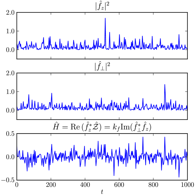
Figure 1: Time series of the random forcing time variances, $|\hat{f}_{z}|^{2}$ and $|\hat{f}_{\perp}|^{2}$, and forcing helicity $\hat{H}(t)$ for a case with $\theta_{f}=\pi/4$, $S=1$, $t_{f}=0.1$, and $\nu=0.1$. The discrete time step size is $\Delta t=0.025$.

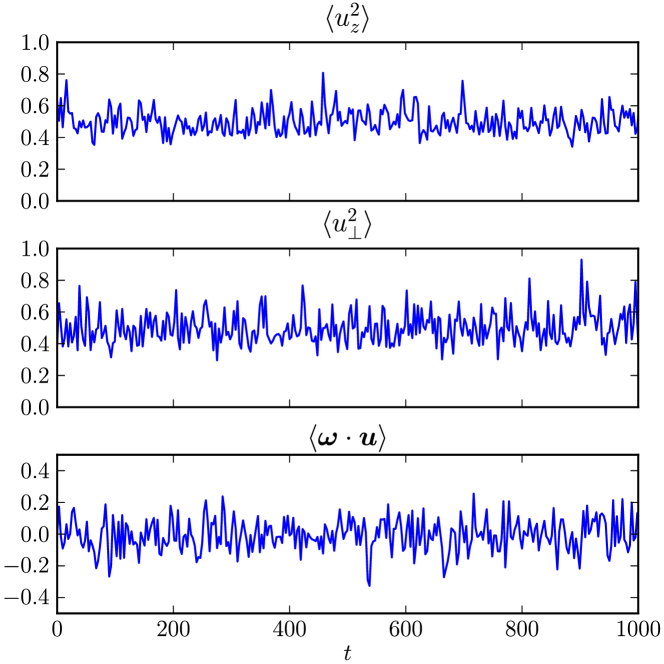
Figure 2: Time series for vertical and horizontal velocity variances (i.e., twice $KE_{z}(t)$ and $KE_{\perp}(t)$) and the associated kinetic helicity response, $\Big{\langle}\,{\bf u}\cdot{\bf\omega}\,\Big{\rangle}^{bfx}\,(t)$, for random velocities generated by the forcings in Fig. 1.

An illustration of a random realization of the forcings, velocity variances, and helicity time series is in Figs. 1-2. These are for a case with moderately up-shear forcing wavenumber orientation ($\theta_{f}=\pi/4$), moderately small correlation time $t_{f}=0.1$ and viscosity $\nu=0.1$, and intermediate mean shear rate ($S=1$). The amplitude normalizations from (35) are evident, as is the vanishing of the time-averaged helicity. Because $t_{f}\nu\ll 1$, the time scale of the velocity fluctuations is controlled primarily by the viscous decay time modified by the shear tilting in the $k_{x}(t)$: in (32) the initial exponential linear decay rate, $\nu=0.1$, is at first slowed as $k_{x}$ passes through zero at $t=1/S\tan\theta_{f}=1$ and then augmented toward a exponential cubic decay with a rate coefficient $\approx\,(\nu S^{2}k_{yf}^{2}/3)^{1/3}=0.26$.

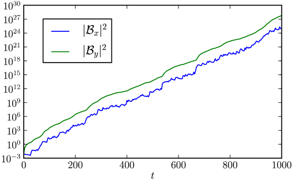
Figure 3: Mean-field variance time series for the same case as in Figs. 1-2. Additional case parameters are $\eta=0.1$, $k_{z}=0.125$, and $\theta_{B}=\pi/4$.

To obtain a dynamo in (65), the vertical wavenumber $k_{z}$ must be small but finite; we show below that this is true for general parameters. With $k_{z}=0.125$ and moderately small $\eta=0.1$, the time series of the mean magnetic field component variances are shown in Fig. 3 for the same realization of the forcing and velocity as in Figs. 1-2. There is evident exponential growth in both components of $\boldsymbol{\mathcal{B}}(t)$, i.e., this is a dynamo. If we make an exponential fit over a long time interval with $|\boldsymbol{\mathcal{B}}|\propto e^{\gamma}t$, we obtain the same value of $\gamma\approx 0.03$ for each component. $\boldsymbol{\mathcal{B}}(t)$ also manifests a stochastic variability inherited from the random forcing, and its fluctuations about the exponential growth exhibit power even at much lower frequencies than are evident in the forcing and velocity time series.

The magnitude of $\mathcal{B}_{y}$ is larger than of $\mathcal{B}_{x}$ in Fig. 3. This is a common behavior for magnetic fields in shear flow. A partial and somewhat simplistic explanation is as a consequence of the first right-side shear term in (65). A simplified (non-dynamo) system with arbitrary forcing $\boldsymbol{R}(t)$,

$$\partial_{t}\boldsymbol{\mathcal{B}}=S\mathcal{B}_{x}\boldsymbol{e}_{y}+\boldsymbol{r}(t)\,,\qquad\boldsymbol{\mathcal{B}}(0)=\boldsymbol{\mathcal{B}}_{0}\\ ,$$ (70)

has the solution,

$$\boldsymbol{\mathcal{B}}(t)=\boldsymbol{\mathcal{B}}_{0}+\int_{0}^{t}\,\mathrm{d}{}t^{\prime}\,\boldsymbol{R}(t^{\prime})+S\boldsymbol{e}_{y}\left(\,\mathcal{B}_{x0}t+\int_{0}^{t}\,\mathrm{d}{}t^{\prime}\,\int_{0}^{t^{\prime}}\,\mathrm{d}{}t^{\prime\prime}\,r_{x}(t^{\prime\prime})\,\right)\,.$$ (71)

The last term $\propto S\boldsymbol{e}_{y}$ will make $|\mathcal{B}_{y}|\gg|\mathcal{B}_{x}$ at late time for most $\boldsymbol{R}(t)$. This anisotropy effect carries over to the ESD but also involves further right-side $\boldsymbol{\mathcal{B}}$ coupling absent in (71); a coupled explanation for the anisotropy in dynamo solutions is made in Sec. 5.1. The initial condition $\boldsymbol{\mathcal{B}}_{0}$ is usually not dominant in (71) at late time. The initial condition is even less important for $\boldsymbol{\mathcal{B}}(t)$ in Fig. 3, which is obtained with $\theta_{B}=\pi/4$; in particular, $\theta_{B}$ does not determine the dynamo growth rate $\gamma$.

$\boldsymbol{b}(t)$ (not shown) also shows exponential growth in its amplitude, with $|b_{y}|$ typically much larger than $|b_{x}|$ for the same reason as just explained. $\boldsymbol{b}(t)$ has comparable time dependence to $u_{z}(t)$ and $\boldsymbol{u}(t)$, as well as an additional resistive decay influence from $\eta$ and modulations by the exponential growth and slow variation in $\boldsymbol{\mathcal{B}}(t)$.

5 Dynamo Analysis in Limiting Cases

5.1 $L\rightarrow\infty$; $\eta,\ \nu\rightarrow\infty$

The ESD in Secs. 3-4 is based on an assumption that the horizontal domain size is large, $L\rightarrow\infty$ (n.b., the average of a Fourier exponential in (40)). As a means of obtaining a more readily analyzed form of the ESD (65), we take the additional limit of $\eta\rightarrow\infty$. This limit does not change the forcing amplitude nor the velocity field (Sec. 3), which are independent of $\eta$, but it allows an elimination of one of the time integrals in the expression for $\boldsymbol{b}$ in (55) and in the equation (65) for $\widetilde{\boldsymbol{\mathcal{B}}}$. It also makes the quasi-linear approximation rigorously accurate because it yields $|\boldsymbol{\delta B}|\ll|\boldsymbol{\mathcal{B}}|$ (as explained after (74)).

The essence of the $\eta\rightarrow\infty$ approximation is that first the order of integration in (65) is reversed,

$$\int^{t}_{0}\,\mathrm{d}{}\lambda\,\int^{\lambda}_{0}\mathrm{d}{}\mu=\int^{t}_{0}\,\mathrm{d}{}\mu\,\int^{t}_{t-\mu}\,\mathrm{d}{}\lambda\,,$$

and then the $\lambda$ integral is performed by assuming that $\widetilde{G}_{\eta}$ is more rapidly varying in $\lambda$ than any of the other integrand factors and furthermore is nonzero only when $\lambda\rightarrow t$, i.e., $t-\lambda=O(\eta^{-1})$. We evaluate this approximation as

$$\int^{t}_{t-\mu}\,\mathrm{d}{}\lambda\,\widetilde{G}_{\eta}(t-\mu,\lambda-\mu)\rightarrow\frac{1}{\eta k^{2}(t-\mu)}$$ (72)

for all $\mu\neq t$ (the integral is zero for $\mu=t$) and set the $\lambda$ arguments of other factors in the integrand to $t$. With this approximation, the $(L,\eta)$-limiting form of (65) becomes

$$\partial_{t}\widetilde{\boldsymbol{\mathcal{B}}}=S\widetilde{\mathcal{B}}_{x}(t)\boldsymbol{e}_{y}-\,\frac{1}{\eta}\,\int^{t}_{0}\,\mathrm{d}{}\mu\ \frac{G_{\nu}^{\dagger 2}(t-\mu)}{k^{2}(t-\mu)}\,$$

$$\qquad\Bigl{[}\,k_{z}^{2}{\cal F}^{\dagger}(\mu)\,\widetilde{\boldsymbol{\mathcal{B}}}(t)\ +2\mathrm{i}k_{z}{\cal H}^{\dagger}(\mu)\ \frac{\boldsymbol{e}_{z}\times\boldsymbol{k}(t-\mu)}{k^{2}(t-\mu)}\ \boldsymbol{k}(t-\mu)\cdot\widetilde{\boldsymbol{\mathcal{B}}}(t)\,\Bigr{]}\,.$$ (73)

This is a purely differential equation for $\widetilde{\boldsymbol{\mathcal{B}}}(t)$; i.e., it matches the common ansatz form in (1), viz.,

$$\partial_{t}\widetilde{\boldsymbol{\mathcal{B}}}=\mathsfbi{L}\cdot\widetilde{\boldsymbol{\mathcal{B}}}(t)\,,$$ (74)

for the identifiable single-time, second-order tensor $\mathsfbi{L}(t)$ that contains a time-history integral in $\mu$ over the random forcing.

An analogous simplification of the expression for $\boldsymbol{b}$ in (55) can be made, with the result that $\boldsymbol{b}\propto 1/\eta$. This gives the important analytic result that the quasi-linear approximation to (4) is asymptotically convergent as $\eta\rightarrow\infty$; the higher harmonics of the shearing-wave Fourier phase ($\pm m\phi$, $m>1$) generated in $\boldsymbol{b}$ by the fluctuation electromotive term are $O(\eta^{-m})$, hence negligible compared to the mean-field term proportional to $\Big{\langle}{\boldsymbol{B}}\Big{\rangle}^{x,y}$ in (53).

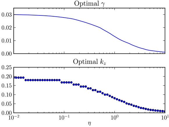
Figure 10: Mean-field growth rate $\gamma$ associated with the optimal $k_{z}$ value as a function of resistivity $\eta$. Other parameters are $\theta_{f}=\pi/4$, $S=1$, $t_{f}=0.1$, $\eta=0.1$, and $\Delta t=0.025$.

Numerical solutions of (73) exhibit dynamo behavior similar to the example in Sec. 4.3, and the parameter dependences for $\gamma$ are similar to those described in Sec. 6 for the general ESD. In particular, $\gamma$ is small here because $\eta$ is large, in contrast to the “fast dynamo” limit where $\gamma$ becomes independent of $\eta$ (cf., Fig. 10).

To obtain further analytic simplicity we can take a sequential limit of (73) as $\nu\rightarrow\infty$. As with the $\eta$ limit, this selects an integration time $\mu\approx t$, where the viscous decay factor is integrated out by the approximate relation for large $t$,

$$\int^{t}_{0}\,\mathrm{d}{}\mu\,G_{\nu}^{2}(t-\mu)\rightarrow\frac{1}{2\nu}\quad{\rm or}\quad\int^{t}_{0}\,\mathrm{d}{}\mu\,G_{\nu}^{\dagger 2}(t-\mu)\rightarrow 1\,,$$ (75)

utilizing the renormalization relations in (41) and (61). The $(L,\eta,\nu)$-limit mean-field equation from (73) is

$$\partial_{t}\widetilde{\boldsymbol{\mathcal{B}}} =S\widetilde{\mathcal{B}}_{x}(t)\boldsymbol{e}_{y}-\,\frac{1}{\eta}\,\Bigl{[}\,k_{z}^{2}{\cal F}^{\dagger}(t)\,\widetilde{\boldsymbol{\mathcal{B}}}(t)\ +2\mathrm{i}k_{z}{\cal H}^{\dagger}(t)\ (\boldsymbol{e}_{z}\times\boldsymbol{k}_{f})\ \boldsymbol{k}_{f}\cdot\widetilde{\boldsymbol{\mathcal{B}}}(t)\,\Bigr{]}\,,$$ (76)

after using $k^{2}(0)=k_{f}^{2}=1$ from (34). In the tensor representation (74), $\mathsfbi{L}(t)$ is defined for (76) by

$$\mathsfbi{L}=S\,\begin{pmatrix}0&0\cr 1&0\cr\end{pmatrix}\,-\,\frac{k_{z}^{2}{\cal F}^{\dagger}(t)}{\eta}\,\begin{pmatrix}1&0\cr 0&1\cr\end{pmatrix}\,-\,\frac{2\mathrm{i}k_{z}{\cal H}^{\dagger}(t)}{\eta}\begin{pmatrix}\cos\theta_{f}\sin\theta_{f}&\sin^{2}\theta_{f}\cr-\,\cos^{2}\theta_{f}&-\,\cos\theta_{f}\sin\theta_{f}\cr\end{pmatrix}\,,$$ (77)

after a substitution for $\boldsymbol{k}_{f}$ from (38). All of the forcing time history in the coefficient tensor $\mathsfbi{L}(t)$ has now disappeared. The history integral also disappears in the companion $\boldsymbol{b}$ formula derived from (55). Furthermore, there is no remaining dependence on $\nu$ in (76) because ${\cal F}^{\dagger}$ and ${\cal H}^{\dagger}$ are $O(1)$ quantities by the $KE$ normalization in (34) and the forcing renormalization in (37) and (61). Large $\eta$ and $\nu$ values lead to momentum and induction equation balances with negligible time tendency terms and negligible shear tilting in $\boldsymbol{k}(t)$ because $\phi\rightarrow\phi_{f}$ and ${\bf k}(t)\rightarrow{\bf k}_{f}$.

We now consider two further limits in the forcing correlation time $t_{f}$ that yield analytic expressions for $\gamma$.

5.1.1 Steady Forcing

Suppose the forcing values taken from the random distributions in Sec. 3.3 but are held steady in time; this is a limit based on the physical approximation that the forcing amplitudes change more slowly than the inverse growth rate for the dynamo, $\gamma t_{f}\gg 1$. In this limit (76)-(77) has its $\mathsfbi{L}$ independent of time, hence there are eigensolutions with

$$\widetilde{\boldsymbol{\mathcal{B}}}\ \propto\ e^{\Gamma t}\,.$$ (78)

The eigenvalues of $\mathsfbi{L}$ are

$$\Gamma=-\,\frac{k_{z}^{2}}{\eta}{\cal F}^{\dagger}\ \pm\ \left(\frac{2\mathrm{i}k_{z}\sin^{2}\theta_{f}{\cal H}^{\dagger}\,S}{\eta}\right)^{1/2}\,.$$ (79)

The dynamo growth rate for total mean field $\boldsymbol{\mathcal{B}}$ is defined as the largest real part of $\Gamma$ plus a correction of $-\,\eta k_{z}^{2}$ from the transformation in (64):

$$\gamma=-\left(\eta+\frac{{\cal F}^{\dagger}}{\eta}\right)\,k_{z}^{2}+\left(\frac{k_{z}|S{\cal H}^{\dagger}|\sin^{2}\theta_{f}}{\eta}\right)^{1/2}\,.$$ (80)

The first term is negative and the second positive. A dynamo occurs with $\gamma>0$ if there are both forcing helicity and shear and if $k_{z}$ is small enough but nonzero. With $S=0$, there is no dynamo. For $|S|$ above a critical-shear threshold value,

$$S_{cr}=\frac{\eta k_{z}^{3}}{\sin^{2}\theta_{f}}\,\frac{(\eta+\eta^{-1}{\cal F}^{\dagger})^{2}}{|{\cal H}^{\dagger}|}>0\,,$$ (81)

$\gamma$ increases with $S$, asymptotically as $\sqrt{S}$ when the other parameters are held constant, and $\gamma$ decreases with $\eta$ as $1/\eta$. For given $S$, there is a lower threshold value for $\eta$ to have a dynamo. Nonzero forcing helicity is necessary for a dynamo, but its sign does not matter. $\gamma=0$ for $k_{z}=0$, and $\gamma<0$ for $k_{z}$ large. Within an intermediate range where $\gamma>0$, the optimal $k_{z}$ and its associated growth rate are

$$k_{z\,opt} =\left(\frac{|S{\cal H}^{\dagger}|\sin^{2}\theta_{f}}{16\,\eta(\eta+\eta^{-1}{\cal F}^{\dagger})^{2}}\right)^{1/3}\approx\ \left(\frac{|S{\cal H}^{\dagger}|\sin^{2}\theta_{f}}{16\,\eta^{3}}\right)^{1/3}$$

$$\gamma_{opt} =\left(\frac{27\,|S{\cal H}^{\dagger}|^{2}\sin^{4}[\theta_{f}]}{256\,\eta^{2}(\eta+\eta^{-1}{\cal F}^{\dagger})}\right)^{1/3}\approx\ \left(\frac{27\,|S{\cal H}^{\dagger}|^{2}\sin^{4}[\theta_{f}]}{256\,\eta^{3}}\right)^{1/3}\,,$$ (82)

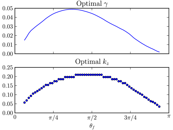
Figure 11: Mean-field growth rate $\gamma$ associated with the optimal $k_{z}$ value as a function of forcing angle $\theta_{f}$. Other parameters are $\theta_{f}=\pi/4$, $S=1$, $t_{f}=0.1$, $\nu=1.0$, and $\Delta t=0.025$.

where the approximations are based on neglecting ${\cal F}^{\dagger})/\eta^{2}$. The optimal $k_{z}$ decreases with increasing $\eta$. (In a general MHD simulation with fixed $(S,\eta,\nu)$ values, all $k_{z}$ are available, and the ones supporting a dynamo will emerge in the evolution.) The vertical forcing variance ${\cal F}^{\dagger}$ reduces the dynamo, while the forcing helicity amplitude $|{\cal H}^{\dagger}|$ enhances it. ${\cal F}^{\dagger}$ enters (77) and (80) exactly as an enhanced resistivity; however, the effect is small as $O(\eta^{-2})$ when ${\cal F}^{\dagger}=O(1)$ in this large $\eta$ limit. This is an anisotropic turbulent eddy resistivity acting on the mean field in the direction perpendicular to the shear plane as a result of the shearing-wave vertical velocity (Parker, 1971; Moffatt, 1978). The horizontal force $\boldsymbol{f}$ acting by itself has no effect; it makes ${\cal F}=|{\cal H}|=0$, hence $\gamma<0$ (no dynamo). $\gamma$ is largest where $k_{yf}$ is largest at $\theta_{f}=\pi/2$; in Sec. 6 we show that $\gamma$ is usually larger for $\theta_{f}<\pi/2$ (Fig. 11) because of a dynamo enhancement by the shear-tilting Orr effect when $\nu<\infty$. $k_{xf}$ does not explicitly enter the formula for $\gamma$ in the present case.

The system (76)-(77) in its steady-helicity limit is a close analog of the so-called alpha–omega dynamo for galactic disks Parker (1971); Kulsrud (2010). Using a mixed notation from these two sources and assuming a vertical structure $\Big{\langle}{\,\boldsymbol{B}\,}\Big{\rangle}^{x,y}\ \propto\ e^{\mathrm{i}k_{z}z}$, an ODE system analogous to (74) results, with

$$\mathsfbi{L}^{\alpha\Omega}=\begin{pmatrix}-\,\widetilde{\eta}k_{z}^{2}&\mathrm{i}k_{z}\alpha\cr\Omega&-\,\widetilde{\eta}k_{z}^{2}\cr\end{pmatrix}\,.$$ (83)

For constant $\alpha$ and $\Omega$, its eigenvalues are

$$\Gamma^{\alpha\Omega}=-\,k_{z}^{2}\widetilde{\eta}\pm\left(\mathrm{i}k_{z}\alpha\Omega\right)^{1/2}\,.$$ (84)

The correspondence with (79) is evident with appropriate identifications between $(\alpha,\ \Omega,\ \widetilde{\eta})$ and $(\eta^{-1}{\cal H}^{\dagger},\ S,\ \eta+\eta^{-1}{\cal F}^{\dagger})$. However, the ODE systems are not isomorphic except in the special case of $k_{xf}=0$ in (74). Thus, in the steady-forcing ESD, the shear $S$ plays the role of $\Omega$, helical forcing ${\cal H}^{\dagger}$ plays the role of $\alpha$, and ${\cal F}^{\dagger}$ plays the role of a turbulent eddy resistivity that augments the effect of $\eta$.

The physical paradigm in this paper is random forcing. Therefore, even if the forcing is steady in time, it is taken from a random distribution, and we can ask what the expected value is for $\widetilde{\boldsymbol{\mathcal{B}}}$ (i.e., having factored out the resistive decay in (64), which is not dominant for small $k_{z}$). To answer this we now neglect the turbulent resistivity by ${\cal F}^{\dagger}$, which is shown above to be a small effect for large $\eta$. The eigenvalue (79) of the tensor (77) is for a particular forcing value, which we now generalize to an ensemble distribution,

$$\Gamma(\varepsilon)=\pm\gamma(1+\mathrm{i}s)\,,\quad\gamma(\varepsilon)=\frac{1}{\sqrt{2}}\,ES\sin\theta_{f}>0\,,$$ (85)

with a composite parameter that is a rescaled helicity forcing,

$$\varepsilon=\frac{2k_{z}{\cal H}^{\dagger}}{S\eta}\equiv E^{2}s\,.$$ (86)

$E^{2}$ is the magnitude of $\varepsilon$, and $s=\pm 1$ is its sign. Consistent with the Ornstein-Uhlenbeck process for the forcing amplitudes (Sec. 3.3), $\varepsilon$ has a Gaussian probability distribution function,

$${\cal P}(\varepsilon)=\frac{1}{\sqrt{2\pi\varepsilon_{0}^{2}}}\ \exp\Bigl{[}-\,\varepsilon^{2}/2\varepsilon_{0}^{2}\Bigr{]}\,,\qquad\int_{-\infty}^{\infty}\,{\cal P}\,\mathrm{d}{}\varepsilon=1\,,$$ (87)

with an expected variance $\varepsilon_{0}^{2}$. Utilizing ${\cal E}\Bigl{[}{\cal H}^{\dagger 2}\Bigr{]}=0.5\,F_{z}\dagger\,O_{z}^{\dagger}=0.5$ from the remark after (37), we obtain

$$\varepsilon_{0}^{2}=\frac{2k_{z}^{2}}{S^{2}\eta^{2}}\rightarrow\frac{1}{4S^{4/3}\eta^{4}}\,,$$ (88)

where the arrow indicates substitution of $k_{z}^{opt}$ from (82). We analyze the dynamo solutions with general $\varepsilon_{0}$, but for large $\eta$, $\varepsilon_{0}$ is expected to be small. After a large elapsed time $t_{e}$, the dynamo solution is dominated by its leading eigenmode with $\mathrm{Re}\left\{\,\Gamma\right\}=\gamma>0$ for any $E\neq 0$. Neglecting the decaying mode, we write the late-time solution in vector form as

$$\begin{pmatrix}\widetilde{\mathcal{B}}_{x}(\varepsilon,t_{e})\cr\widetilde{\mathcal{B}}_{y}(\varepsilon,t_{e})\cr\end{pmatrix}\ =\ {C}_{0}\,e^{\gamma t_{e}}\,\left(\cos[\gamma t_{e}]+is\sin[\gamma t_{e}]\right)\ \begin{pmatrix}(1+\mathrm{i}s)\gamma/S+\mathrm{i}\varepsilon\cos\theta_{f}\sin\theta_{f}\cr 1-\mathrm{i}\varepsilon\cos^{2}\theta_{f}\cr\end{pmatrix}\,.$$ (89)

${C}_{0}$ is a complex constant determined from the initial condition,

$${C}_{0}=\frac{1}{\sqrt{2}E(i+\mathrm{i}s)}\,\left\{\,\widetilde{\mathcal{B}}_{x}(0)+\widetilde{\mathcal{B}}_{y}(0)\,\left(\frac{(1+\mathrm{i}s)\gamma/S-\mathrm{i}\varepsilon\cos\theta_{f}\sin\theta_{f}}{1-\mathrm{i}\varepsilon\cos^{2}\theta_{f}}\right)\,\right\}\,.$$ (90)

With (87) and (89), we can evaluate the expected value of any property of $\widetilde{\boldsymbol{\mathcal{B}}}(t_{e})$ and its corresponding distribution $D$ with $\varepsilon$; e.g., for the mean-field vector magnitude,

$$B^{rms}\,\equiv\,{\cal E}\Big{[}\,|\widetilde{\boldsymbol{\mathcal{B}}}|\,(t_{e})\,\Big{]}\,=\,\int_{-\infty}^{\infty}\,|\widetilde{\boldsymbol{\mathcal{B}}}|(\varepsilon,t_{e})\,{\cal P}(\varepsilon)\,\mathrm{d}{}\varepsilon\equiv\int_{-\infty}^{\infty}\,D[\,|\widetilde{\boldsymbol{\mathcal{B}}}|\,]\,\mathrm{d}{}\varepsilon\,.$$ (91)

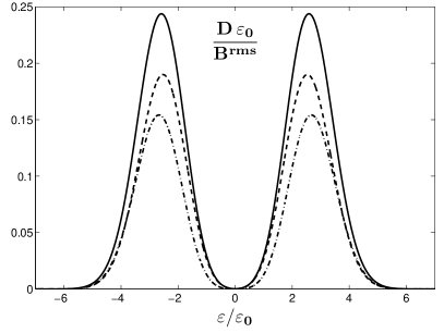
Figure 4: Steady-forcing normalized distributions $D(\varepsilon)$ for (left) $|\widetilde{\boldsymbol{\mathcal{B}}}|$ (solid) and the component magnitudes, $|\widetilde{\mathcal{B}}_{x}|$ (dash-dot) and $|\widetilde{\mathcal{B}}_{y}|$ (dash), and for (right) $\mathrm{Re}\left\{\,\widetilde{\mathcal{B}}_{x}\,\right\}$ (solid) and $\mathrm{Im}\left\{\,\widetilde{\mathcal{B}}_{y}\,\right\}$ (dash) for $S\sqrt{\varepsilon_{0}}\sin\theta_{f}\,t_{e}=6$ and $\varepsilon_{0}=0.1$. This case has $\theta_{f}=\theta_{B}=\pi/4$.

Figure 4 (left panel) shows the distributions $D$ for the vector magnitude and for the directional component magnitudes for a small value of $\varepsilon_{0}$. These distributions are smooth, positive, symmetric in $s$, and peak at intermediate $\varepsilon/\varepsilon_{0}$. $B^{rms}$ and the component magnitudes are growing exponentially with time. We can fit this with a cumulative growth rate, $\gamma^{rms}=t_{e}^{-1}\,\log B^{rms}$, which we know from (85) will scale as $S\sqrt{\varepsilon_{0}}\sin\theta_{f}$. For this value of $\varepsilon_{0}=0.1$, $|\widetilde{\mathcal{B}}_{x}|$ is smaller than $|\widetilde{\mathcal{B}}_{y}|$, with a ensemble-mean ratio of 0.78. For the leading eigenfunction in (89), the anisotropy ratio is

$$\frac{|\widetilde{\mathcal{B}}_{x}|}{|\widetilde{\mathcal{B}}_{y}|}=\frac{(1+\mathrm{i}s)E\sin\theta_{f}+\mathrm{i}\sqrt{2}\varepsilon\cos\theta_{f}\sin\theta_{f}}{\sqrt{2}(1-\mathrm{i}\varepsilon\cos^{2}\theta_{f})}\,.$$ (92)

For small $E$, the ratio tends to $E\sin\theta_{f}/\sqrt{2}$, which is small; this is consistent with the anisotropy in Fig. 3. For large $E$, the ratio tends to $|\tan\theta_{f}|$, which can have any value.

What is the ensemble-mean magnetic field? Its magnitude is

$$B^{mean}\,\equiv\,\Big{|}\,{\cal E}\Big{[}\,\widetilde{\boldsymbol{\mathcal{B}}}(t_{e})\,\Big{]}\,\Big{|}\,=\,\Big{|}\,\int_{-\infty}^{\infty}\,\widetilde{\boldsymbol{\mathcal{B}}}(\varepsilon,t_{e})\,{\cal P}(\varepsilon)\,|\,\mathrm{d}{}\varepsilon\,\Big{|}\,\equiv\,\Big{|}\,\int_{-\infty}^{\infty}\,D[\,\widetilde{\boldsymbol{\mathcal{B}}}\,]\,\mathrm{d}{}\varepsilon\,\Big{|}\,.$$ (93)

Again this is evaluated with (89). We find that it too exhibits exponential growth, so we fit a cumulative growth rate, $\gamma^{mean}(t_{e})=t_{e}^{-1}\,\log B^{mean}>0$. But the ensemble mean growth is smaller than the ensemble r.m.s. growth, i.e., $\gamma^{mean}<\gamma^{rms}$. The reason is illustrated in Fig. 4 (right panel) for the distributions of two components, $D[\,\mathrm{Re}\left\{\,\widetilde{\mathcal{B}}_{x}\,\right\}\,]$ and $D[\,\mathrm{Im}\left\{\,\widetilde{\mathcal{B}}_{y}\,\right\}\,]$. Their amplitude is comparable to the magnitude distributions in the left panel, but they are oscillatory in $\varepsilon$ as a result of $\cos[\gamma t_{e}]$ and $\sin[\gamma t_{e}]$ terms in (89). So the expected value from integration over $\varepsilon$ is small, although not zero. For Fig. 4, $B^{mean}=0.073B^{rms}$, and $\gamma^{mean}=0.76\gamma^{rms}$.

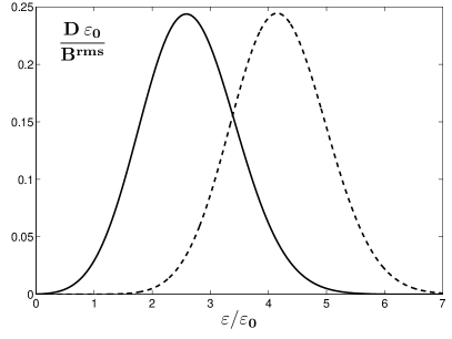
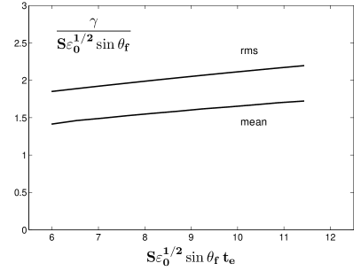
Figure 5: (Left) steady-forcing normalized distributions $D(\varepsilon)$ for $|\widetilde{\boldsymbol{\mathcal{B}}}|$ at two times: $S\sqrt{\epsilon_{0}}\sin\theta_{f}\,t_{e}=6$ (solid) and $12$ (dash). Case parameters are as in Fig. 4. (Right) steady-forcing normalized growth rates, $\gamma^{rms}$ and $\gamma^{mean}$, as a function of evaluation time $t_{e}$.

These relations are not sensitive to the initial condition $\widetilde{\boldsymbol{\mathcal{B}}}(0)$, although it does influence the partition among the real and imaginary parts of $\widetilde{\boldsymbol{\mathcal{B}}}(t_{e})$. There are the expected dependences of larger $\gamma$ with larger $S$ and $\varepsilon_{0}$ and with $\theta_{f}$ closer to $\pi/2$, as in (80). With larger $t_{e}$ the expected values are dominated by the farther tails of the $D$ distributions, with slowly increasing $\gamma^{rms}(t_{e})$ and $\gamma^{mean}(t_{e})$ associated with larger $\gamma(\epsilon)$ in the tails (Fig. 5). Even though larger $\epsilon$ values are less probable in $P(\varepsilon)$ in (87), they do have a more than compensating stronger dynamo growth rate that emerges after long enough time. Because the discrepancy between $\gamma^{rms}$ and $\gamma^{mean}$ persists even in the $P(\varepsilon)$ tail, the ratio $B^{mean}/B^{rms}$ decreases with $t_{e}$ exponentially. The steady-forcing dynamo does not become independent of $t_{e}$ as $t_{e}\rightarrow\infty$, in contrast to the finite-$t_{f}$ dynamo, in particular the small-$t_{f}$ dynamo analyzed in Sec. 5.1.2.

5.1.2 Rapidly Varying Forcing

The limiting forms for the ESD equation, (73) and (76), are also analyzable in the opposite limit of $t_{f}\rightarrow 0$ by means of a cumulant expansion of a linear, stochastic, ODE system (van Kampen, 2007, Chap. XVI). For a stochastic vector $\boldsymbol{A}(t)$ governed by

$$\partial_{t}\boldsymbol{A}=\left(\,\mathsfbi{L}_{0}+\mathsfbi{L}_{1}(t)\,\right)\,\cdot\boldsymbol{A}\,,$$ (94)

with the tensors $\mathsfbi{L}_{0}$ independent of time and $\mathsfbi{L}_{1}(t)$ a random stationary process with zero expected mean and finite variance, the expected value ${\cal E}\Big{[}\boldsymbol{A}\Big{]}$ satisfies the approximate deterministic ODE system,

$$\partial_{t}{\cal E}\Big{[}\boldsymbol{A}\Big{]}=\left(\,\mathsfbi{L}_{0}+\int_{0}^{\infty}\,{\cal E}\Big{[}\mathsfbi{L}_{1}(t)\,\mathsfbi{L}_{1}(t-t^{\prime})\Big{]}\,dt^{\prime}+\dots\,\right)\,\cdot{\cal E}\Big{[}\boldsymbol{A}\Big{]}\,,$$ (95)

with the dots indicating neglected higher-order cumulant terms. The system (95) has a time-independent matrix; hence, it has eigenmodes with exponential time dependence with growth rates given by the matrix eigenvalues. The solution formula for ${\cal E}\Big{[}{\bf A}\Big{]}(t)$ is called a time-ordered exponential matrix, and it has a non-terminating series expansion with the leading terms as indicated here. The basis for the approximate neglect of the higher order terms can be taken as the vanishing of ${\cal E}\Big{[}\mathsfbi{L}_{1}1(t)\,\mathsfbi{L}_{1}(t-t^{\prime})\Big{]}$ except as $|t-t^{\prime}|\rightarrow 0$. In the present situation with large $\nu$, this is equivalent to short correlation times $t_{f}\rightarrow 0$ for the random forces, $\hat{f}_{z}(t)$ and $\hat{o}_{z}(t)$, with $St_{f}\ll 1$ and $S/\nu\ll 1$ to be able to neglect higher-order products of $\mathsfbi{L}_{0}$ and $\mathsfbi{L}_{1}$ in deriving (95).

We apply (94)-(95) to (76) with $\boldsymbol{A}=\widetilde{\boldsymbol{\mathcal{B}}}\,\exp\Bigl{[}k_{z}^{2}{\cal F}_{0}^{\dagger}t/\eta\Bigr{]}$ with the following tensors:

$$\mathsfbi{L}_{0}=S\,\begin{pmatrix}0&0\cr 1&0\cr\end{pmatrix}\,,\quad\mathsfbi{L}_{1}=\frac{2\mathrm{i}k_{z}{\cal H}^{\dagger}(t)}{\eta}\,\begin{pmatrix}\cos\theta_{f}\sin\theta_{f}&\sin^{2}\theta_{f}\cr-\,\cos^{2}\theta_{f}&-\,\cos\theta_{f}\sin\theta_{f}\cr\end{pmatrix}\,.$$ (96)

This is a second-order, complex system. We have made one ad hoc simplification here, viz., replacing ${\cal F}^{\dagger}(t)$ by its expected value, ${\cal F}_{0}^{\dagger}\equiv{\cal E}\Big{[}{\cal F}^{\dagger}\Big{]}=0.5$ from (61), and then factoring its decay effect on $\widetilde{\boldsymbol{\mathcal{B}}}$ analogously to (64). The motivation is to simplify the analysis. We already understand ${\cal F}$ as an eddy resistive damping. This role is played with qualitative fidelity by retaining only its mean value, and anyway for large $\eta$ it is only a small increment to the ordinary resistivity. The result for (95) is very simple with (96) because $\mathsfbi{L}_{1}^{2}=0$ independent of its time-variable prefactor, and the eigenvalues of $\mathsfbi{L}_{0}$ are zero. Hence, again after restoring the resistive decay factors, the growth rate for ${\cal E}\Big{[}\boldsymbol{\mathcal{B}}\Bigr{]}$ is

$$\gamma=-\,\left(\eta+\frac{1}{2\eta}\right)\,k_{z}^{2}\leq 0\,;$$ (97)

i.e., in this ($\eta\rightarrow\infty$, $t_{f}\rightarrow 0$) limit there is only resistive decay of the expected value of the mean magnetic field, weakly augmented by the eddy resistive effect.

We could continue the cumulant expansion for $\boldsymbol{\mathcal{B}}$ and (94) to higher orders in $St_{f}$ and $S/\nu$ (van Kampen, 2007), seeking growth in the ensemble-mean, large-scale field, ${\cal E}\Big{[}\boldsymbol{\mathcal{B}}\Bigr{]}$, but its $\gamma$ would be small in these parameters compared to the growth in the mean magnetic variance, ${\cal E}\Big{[}\,|\boldsymbol{\mathcal{B}}|^{2}\,\Bigr{]}$. To obtain a dynamo result for the latter, we instead apply (94)-(95) to the fourth-order real covariance system derived from (73) for the vector,

$$\boldsymbol{A}=\left(\ |\widetilde{B}_{x}|^{2},\ |\widetilde{B}_{y}|^{2},\ \mathrm{Re}[\widetilde{B}_{x}^{\ast}\widetilde{B}_{y}],\ \mathrm{Im}[\widetilde{B}_{x}^{\ast}\widetilde{B}_{y}]\ \right)\,\times\,\exp\Bigl{[}2k_{z}^{2}{\cal F}_{0}^{\dagger}t/\eta\Bigr{]}\,,$$ (98)

again factoring out the mean eddy resistive effect with the simplification ${\cal F}^{\dagger}(t)\approx{\cal F}^{\dagger}_{0}=0.5$. The associated tensors are defined by

$$\mathsfbi{L}_{0}=S\mathsfbi{L}_{0}^{\dagger},\,\mathsfbi{L}_{0}^{\dagger}=\begin{pmatrix}0&0&0&0\cr 0&0&2&0\cr 1&0&0&0\cr 0&0&0&0\cr\end{pmatrix}\,,$$

$$\mathsfbi{L}_{1}=\frac{-2k_{z}{\cal H}^{\dagger}(t)}{\eta}\mathsfbi{L}_{1}^{\dagger},\,\mathsfbi{L}_{1}^{\dagger}=\begin{pmatrix}0&0&0&2\sin^{2}\theta_{f}\cr 0&0&0&2\cos^{2}\theta_{f}\cr 0&0&0&-2\cos\theta_{f}\sin\theta_{f}\cr\cos^{2}\theta_{f}&\sin^{2}\theta_{f}&2\cos\theta_{f}\sin\theta_{f}&0\cr\end{pmatrix}.$$ (99)

The expectation value in (95) applied to $\mathsfbi{L}_{1}(t)\mathsfbi{L}_{1}(t-t^{\prime})$ acts entirely on its scalar prefactor in (99) because its matrix factor $\mathsfbi{L}_{1}^{\dagger}$ is deterministic and time-independent. We evaluate the corresponding scalar prefactor that arises in (95) as

$$\frac{4k_{z}^{2}}{\eta^{2}}\,\int_{0}^{\infty}\,{\cal E}\Big{[}{\cal H}^{\dagger}(t){\cal H}^{\dagger}(t-t^{\prime})\Bigr{]}\,dt^{\prime}\,.$$

Tracing backwards through the forcing relations (28), (37), and (61), we derive

$${\cal E}\Big{[}{\cal H}^{\dagger}(t){\cal H}^{\dagger}(t-t^{\prime})\Bigr{]}=0.5\,{\cal E}\Bigl{[}|\hat{f}_{z}^{\dagger}|^{2}\Bigr{]}\,{\cal E}\Bigl{[}|\hat{o}_{z}^{\dagger}|^{2}\Bigr{]}\,\exp\Bigl{[}-2|t^{\prime}|/t_{f}\Bigr{]}\,,$$ (100)

utilizing the fact that the real and imaginary parts of $\hat{f}_{z}$ and $\hat{o}_{z}$ are independent, stationary processes each with an exponential correlation time $t_{f}$ as in (29). After performing the time integration with this expression, the value of the preceding prefactor is

$$\frac{2k_{z}^{2}\,t_{f}}{\eta^{2}}\,{\cal E}\Bigl{[}{\cal H}^{\dagger 2}\Bigr{]}=\frac{k_{z}^{2}\,t_{f}}{\eta^{2}}\,,$$ (101)

because ${\cal E}\Bigl{[}{\cal H}^{\dagger 2}\Bigr{]}=0.5\,F_{z}\dagger\,O_{z}^{\dagger}=0.5$ from (37). This completes the specification of the deterministic, time-independent matrix in (95) for the covariance system as

$$\mathsfbi{L}=S\mathsfbi{L}_{0}^{\dagger}+\frac{k_{z}^{2}\,t_{f}}{\eta^{2}}\mathsfbi{L}_{1}^{\dagger 2}\,.$$ (102)

We evaluate its eigenvalues $\Gamma$ analytically from $det[\mathsfbi{L}-\Gamma\mathsfbi{I}]=0$, which is a fourth-order polynomial equation. We can factor a $\Gamma=0$ root, leaving a third-order system with the reduced form of $\Gamma^{3}+p\Gamma=q$ for coefficients $p\propto S$ and $q\propto S^{2}$. With a simplification provided by the prefactor (101) being small compared to $S$, we can neglect the $p$ term and obtain the approximate solution,

$$\Gamma\approx q^{1/3}=\left(\,\frac{2k_{z}^{2}S^{2}\sin^{4}\theta_{f}\,t_{f}}{\eta^{2}}\right)^{1/3}\,.$$ (103)

This approximation is consistent with finite $S$, small $t_{f}$ and $k_{z}$, and large $\eta$; recall that we also assume $St_{f},\ S/\nu\ll 1$ for the leading order cumulant approximation (95). The three solutions (103) are one with real, positive $\Gamma$ (i.e., a dynamo) and a complex conjugate pair with $\mathrm{Re}[\Gamma]<0$. We divide the positive eigenvalue $\Gamma$ by 2 and restore the resistive decay factors to obtain the growth rate for the r.m.s. value of the mean field, $\left(\,{\cal E}\Big{[}|\boldsymbol{\mathcal{B}}|^{2}\Bigr{]}\,\right)^{1/2}$:

$$\gamma=-\,\left(\eta+\frac{1}{2\eta}\right)k_{z}^{2}\ +\ \left(\,\frac{k_{z}^{2}S^{2}\,\sin^{4}\theta_{f}\,t_{f}}{4\eta^{2}}\,\right)^{1/3}\,.$$ (104)

A dynamo can occur with $\gamma>0$ if there are both forcing helicity and shear and if $k_{z}$ is small but nonzero; this behavior is the same as in the steady-forcing dynamo (80) for this same limiting ESD system (76), as well as for the general dynamo in Sec. 6. In this limit of small correlation time with zero mean helicity and finite helicity variance, the expected value for the mean field $\boldsymbol{\mathcal{B}}$ does not grow, but the expected value for the mean magnetic energy $\boldsymbol{\mathcal{B}}^{2}$ does. The steady-forcing dynamo also has a much smaller ensemble mean than r.m.s. (Sec. 5.1.1).

Besides the leading eigenvalue (103), we can obtain the associated eigenfunction for the matrix (102). With the same approximation of a small prefactor for $\mathsfbi{L}^{\dagger 2}$, we derive the following for the expected ratio of component variances,

$${\cal E}\Bigl{[}|\widetilde{B}_{x}|^{2}\Bigr{]} \approx\frac{2\sin^{4}\theta_{f}}{\Gamma}\ {\cal E}\Bigl{[}|\widetilde{B}_{y}|^{2}\Bigr{]}$$

$$=\left(\frac{2k_{z}^{2}\sin^{4}\theta_{f}t_{f}}{S\eta^{2}}\right)^{2/3}\,{\cal E}\Bigl{[}|\widetilde{B}_{y}|^{2}\Bigr{]}\,.$$ (105)

Thus, the streamwise mean magnetic energy is small compared to the transverse energy in the present limit with transient forcing, small $k_{z}$ and $t_{f}$, and large $\eta$. The small ratio is also consistent with the previous example of dynamo behavior with more general parameters in Fig. 3, as well as with the steady-forcing dynamo in Sec. 5.1.1 when $\varepsilon_{0}$ is small.

As with the steady forcing (82) we can optimize the growth rate in $k_{z}$:

$$k_{z\,opt} =\left(\,\frac{S^{2}\sin^{4}\theta_{f}\,t_{f}}{108\,\eta^{2}\,(\eta+\frac{1}{2\eta})^{3}}\,\right)^{1/4}$$

$$\gamma_{opt} =\left(\,\frac{S^{2}\sin^{4}\theta_{f}\,t_{f}}{27\,\eta^{2}(\eta+\frac{1}{2\eta})}\,\right)^{1/2}\,.$$ (106)

The parameter tendencies here all have the same signs as with steady-forcing and with the general ESD (Sec. 6), but the exponents are different in the two $t_{f}$ limits. In particular, the optimal growth rate dependences are

$$\gamma \sim\ S\ \ ||{\cal H}||\,\eta^{-3/2}\,k_{yf}^{2}\,t_{f}^{1/2}\qquad\quad{\rm as}\ t_{f}\rightarrow 0$$

$$\gamma \sim\ S^{2/3}\,||{\cal H}^{\dagger}||^{2/3}\,\eta^{-1}\,k_{yf}^{4/3}\,t_{f}^{0}\qquad{\rm as}\ t_{f}\rightarrow\infty\,,$$ (107)

where the norm symbol $||\cdot||$ denotes the r.m.s. or mean magnitude as appropriate, and we have formally restored the helicity variance factor $||{\cal H}||$ for emphasis. In both cases the growth rate $\gamma$ is vanishingly small as $\eta\rightarrow\infty$, $S\rightarrow 0$, $||{\cal H}||\rightarrow 0$, or $\theta_{f}\rightarrow 0,\pi$, and for the short correlation time case, $\gamma$ is small as $t_{f}\rightarrow 0$. For non-limiting values of the parameters, however, $\gamma$ is not small (Sec. 6). We reiterate that there is no dependence of $\gamma$ on $\nu$ in the limit $\nu\rightarrow\infty$, independent of the value of $t_{f}$.

As with the steady forcing limit, an analogy exists between the fluctuating helicity ESD in (76) and a low-order ODE fluctuating alpha–omega dynamo ansatz (Vishniac & Brandenburg, 1997; Silant’ev, 2000) (also called the incoherent alpha–shear dynamo). Therefore, from a historical perspective of astrophysical dynamo theory, we see that the ESD in (63) provides both a theoretical justification for the alpha–omega ansatz, with an explicit characterization of the relevant shearing-wave velocity fluctuations, and a generalization to finite Reynolds numbers (i.e., $\eta,\nu<\infty$).

In summary, these two different $t_{f}$ limits with analytic dynamo solutions for the large-$(\eta,\nu)$ ESD (76) show qualitatively similar but functionally different parameter tendencies in $S$, $\eta$, $k_{z}$, and $\theta_{f}$; anisotropy with $|\widetilde{\mathcal{B}}_{y}|$ usually larger than $|\widetilde{\mathcal{B}}_{x}|$; and an ensemble-mean magnetic energy, ${\cal E}\Bigl{[}\,|\widetilde{\boldsymbol{\mathcal{B}}}|^{2}\,\Bigr{]}$, much larger than the energy of the ensemble-mean field, $|\,{\cal E}\Bigl{[}|\widetilde{\boldsymbol{\mathcal{B}}}\Bigr{]}\,|^{2}$. These characteristics carry over to the more general ESD solutions in Sec. 6.

5.2 Other Limit Pathways

The preceding ESD derivation of (65) assumes $k_{yf}L\gg 1$ to assure $\Big{\langle}{exp[\mathrm{i}(\phi+\phi^{\prime})]}\Big{\rangle}^{x,y}\approx 0$ and $k_{yf}LS\ {\rm min}[t_{f},\ 1/\nu]\gg 1$ to assure $\Big{\langle}{exp[\mathrm{i}(\phi+\phi^{\prime})]}\Big{\rangle}^{x,y}\neq 0$ for selected time arguments of the phases $\phi(\mu)$ and $\phi(\mu^{\prime})$. The latter assumption yields (40), which is useful in simplifying the normalization condition (36) for $KE$ and compacting the ESD equation (65) for $\widetilde{\boldsymbol{\mathcal{B}}}$ by reducing the number of time history integrals in the mean electromotive force curl (Appendix A). We prefer the physical rationale of this pathway based only on a primary assumption of large $L$, consistent with uniform mean shear and no boundary conditions, because it does not constrain the values of the other parameters that are physically more meaningful than $L$. The result is independent of $L$ itself. The further ESD simplifications in Sec. 5.1 follow from $\eta,\nu\rightarrow\infty$.

However, this is not a unique pathway for deriving ESD equations that are essentially similar. In particular, neither of the limits $S\rightarrow 0$ nor $t_{f}\rightarrow 0$ is problematic even though they appear inconsistent with the second assumption above. As previously explained, we do require $\nu>0$ for statistical equilibration of velocity fluctuations and $k_{yf}\neq 0$ for nontrivial shear tilting and dynamo behavior.

Shear tilting makes $\phi(t)$ in (20) or (31) a continuous function of time. When $S=0$, $\phi=\phi_{f}$, and the average of the differenced-phase factor is $\Big{\langle}{exp[\mathrm{i}(\phi-\phi^{\prime})]}\Big{\rangle}^{x,y}=1$ for all time arguments. When $S\rightarrow 0$ as a primary assumption, this relation is approximately true. We still require the weaker assumption about large domain size, $k_{yf}L\gg 1$, to be able to neglect the summed-phase factors, $\Big{\langle}{exp[\mathrm{i}(\phi+\phi^{\prime})]}\Big{\rangle}^{x,y}$. Even with these phase averaging relations resolved, further assumptions are needed to compact the electromotive forcing, and large $\eta$ and/or $\nu$ suffice. The outcome is equivalent to (76) with dynamo solutions when $S>0$. If instead the primary assumption is $t_{f}\rightarrow 0$ in combination with $k_{yf}L\gg 1$, then the requirement on the average of the differenced-phase factor in the $KE$ normalization is resolved with an approximate integral over the forcing correlation factor, $\exp[-|\mu-\mu^{\prime}|/t_{f}]$, in (36), but this assumption is not enough to compact the electromotive force curl. Again this can be accomplished with additional assumptions of large $\eta$ and/or $\nu$, leading to the equivalents of (73) with shear tilting and (76) without it. In neither of these limits is there a compact equivalent to the general ESD (65) with finite $\eta$ and $\nu$. Also, because the dynamo solutions of (76) have $\gamma$ small with $S$ and $t_{f}$, this derivation pathway is not as physically germane as the primary one in Sec. 5.1.

Yet another derivation pathway assumes finite $L$ and spatially periodic boundary conditions in shearing coordinates with discretized shearing-frame wavenumbers with $\Delta k=2\pi/L$. If the forcing is at one of the discretized wavenumbers at least in $k_{yf}$, then the spatial average of the summed-phase factor vanishes. To accommodate continuous shear tilting in the finite Fourier series representation, the forcing amplitude time series is viewed as impulses at discrete times, $t_{m}=t_{0}+m\Delta t$, $\Delta t=2\pi/Sk_{yf}L$, $m=0,1,2,\dots$, when a discrete shearing-frame $x$-wavenumber $k_{xm}=k_{xf}+Sk_{yf}t_{m}$ (or its periodic alias) coincides with $k_{xf}$ in the laboratory frame. (This discretization is the one used in a MHD computational code with a finite number of Fourier modes (Yousef et al., 2008a).) This allows the shearing-coordinate spatial average of the differenced-phase factors to have the requisite property for a compact ESD derivation. The resulting ESD replaces the time-history integrals with finite sums over $m$ at discrete forcing times $t_{m}$, and it replaces the continuous laboratory-frame $\boldsymbol{k}(t-\mu)$ with $\boldsymbol{k}(t-t_{m})$. This pathway retains the familiar dependence on $L$ for a discrete Fourier series; this dependence disappears as $L\rightarrow\infty$ when the shearing-periodicity pathway merges with the large-domain pathway as $\Delta k$ and $\Delta t$ vanish. The general behaviors of the finite-$L$ shearing-periodicity ESD and $L\rightarrow\infty$ ESD in (65) are essentially the same. Because of the simplicity of the spatial averaging with the shearing-periodic boundary conditions and the analytical advantages of the assumptions of large $\eta$ and $\nu$, small $S\neq 0$, and small $t_{f}$, a proof-of-concept ESD exposition is in Heinemann et al. (2011a). Its solution coincides with Sec. 5.1.2. Notice that this combined pathway achieves spatial homogeneity even without the enlarged ensemble of uniform mean flows in $\boldsymbol{V}$ (Sec. 3.5).

6 General Parameter Dependences

With the normalization conditions (34)-(35), the non-dimensional parameters of the ESD equation (65) are $S$, $\nu$, $t_{f}$, $\theta_{f}$, $k_{z}$, $\eta$, and $\theta_{B}$. A priori we are interested in possible dynamo behavior over their full ranges. Section 4.3 shows a typical “mid-range” example by computational integration, and Sec. 5 has analytic formulas for the parameter dependences of the growth rate $\gamma$ in two asymptotic limits associated with $\eta,\nu\rightarrow\infty$ and $t_{f}\rightarrow 0$ or $\infty$. In this section we survey the parameters space computationally to show that $\gamma$ in the ESD solution is a smooth, simple function of all its parameters.

For given parameters, a computational solution provides a particular realization of the random forcing in Sec. 3.3. When there is exponential growth in $|\boldsymbol{\mathcal{B}}(t)|$, a fit $\propto e^{\gamma}t$ is made over a long integration period (e.g., $S\Delta t=10^{3}$ in Fig. 3). The $\gamma$ value varies from one realization to another, but the results we report here are fairly well determined, as indicated by the smoothness of parameter curves based on separate estimations at separate parameters. Nevertheless, it is computationally laborious to obtain an ensemble perspective over many realizations.

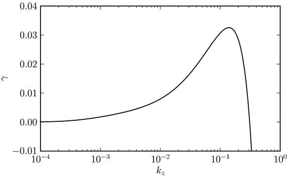
Figure 6: Mean-field growth rate $\gamma$ as a function of $k_{z}$. Parameter values are $S=1$, $\theta_{f}=\pi/4$, $t_{f}=0.1$, $\nu=0.1$, and $\eta=0.1$.

Dynamo growth occurs for finite values of $0<k_{z}<k_{f}=1$ (Fig. 6); i.e., increasing $k_{z}$ amplifies the fluctuating helical forcing in (65) that is essential to the ESD, and dynamo growth is quenched by resistive decay when $k_{z}$ is too large. There is an optimal intermediate value for $k_{z}$ where $\gamma$ is a maximum. This behavior is approximately the same as evident in the analytic solutions in Secs. 5.1.1 and 5.1.2.

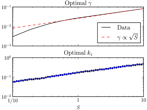
Figure 7: Mean-field growth rate $\gamma$ associated with the optimal $k_{z}$ value as a function of shear $S$. Other parameters are $\theta_{f}=\pi/4$, $t_{f}=0.1$, $\nu=0.1$, and $\eta=0.1$. The dots here (and in subsequent figures) indicate the sampling density for this evaluation of the ESD.

The functional dependence of $\gamma$ on the shear $S$ is in Fig. 7, based on optimization over $k_{z}$ with the other parameters held fixed. The dynamo growth rate increases monotonically with $S$; the slope of $\gamma(S)$ decreases for larger $S$. A power-law fit to $\gamma(S)$ shows an exponent approximately in the range 0.5–1, which is consistent with the values of 2/3 and 1 in the limiting formulas (82) and (106)

The associated optimal $k_{z}(S)$ is always small relative to $k_{f}=1$, and it too increases with $S$. A power law fit shows an exponent similar to the limit values of 1/2 and 1/3 in (82) and (106). In the ESD there is no threshold in $S$ for dynamo growth, given sufficiently small $k_{z}\neq 0$. With either $S=0$ or $k_{z}=0$, there is no dynamo. $\gamma(k_{z})$ is a convex function of $k_{z}$ that vanishes when $k_{z}$ is not small as well as when $k_{z}\rightarrow 0$; this is a similar shape as in the limit formulas (80) and (104). For all other parameters held fixed (including $k_{z}$), there is a minimum threshold value of $S$ for dynamo action, as is also true in the limit formulas (80) and (104).

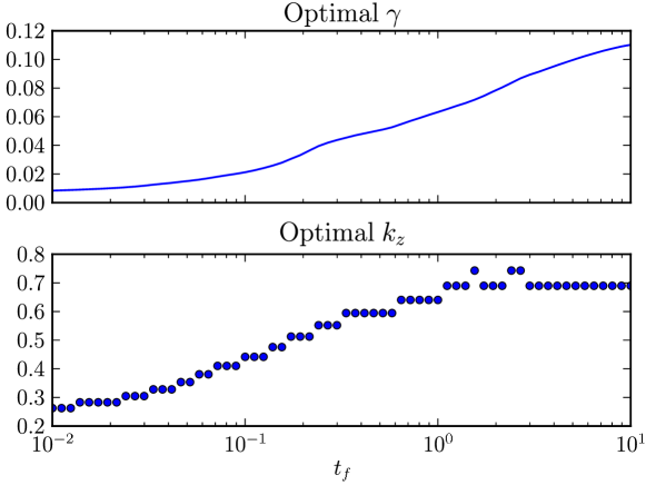
Figure 8: Mean-field growth rate $\gamma$ associated with the optimal $k_{z}$ value as a function of forcing correlation time $t_{f}$. Other parameters are $\theta_{f}=\pi/4$, $S=2$, $\nu=10$, $\eta=0.01$, and $\Delta t=0.01$.

The dependence of $\gamma$ on the forcing correlation time $t_{f}$ is in Fig. 8, again based on optimization over $k_{z}$. $\gamma$ and $k_{z}$ both increase with $t_{f}$. This tendency is consistent at small $t_{f}$ with the limit formulas in (106). For larger $t_{f}$ values the slope of $\gamma(t_{f})$ increases with $t_{f}$ in the range surveyed here, although we know from (82) that $\gamma$ asymptotes to a finite value with steady forcing. The optimal $k_{z}(t_{f})$ levels off with large $t_{f}$, here at a value only slightly smaller than $k_{f}=1$; this behavior is not anticipated by the limit formulas in Sec. 5 that indicate small $k_{z}$ for large $\eta$.

We demonstrate the roles of the forcing components $\hat{f}_{z}$ and $\hat{o}_{z}$ by alternately setting them to zero. $\hat{o}_{z}=0$ removes all forcing from (65), hence has no effect on $\boldsymbol{\mathcal{B}}$. $\hat{f}_{z}=0$ retains the forcing in ${\cal F}$ but makes ${\cal H}=0$; in this case $\boldsymbol{\mathcal{B}}(t)$ shows algebraic growth in time but no dynamo. Thus, a dynamo requires both $u_{z}$ and $\boldsymbol{u}_{\perp}$ to be nonzero. By keeping both components non-zero but arbitrarily setting ${\cal F}=0$ with ${\cal H}\neq 0$ in (65), $\gamma$ is modestly increased; this confirms the interpretation of the ${\cal F}$ effect as turbulent resistivity that weakens dynamo growth (Sec. 5). If ${\cal F}(t)$ is replaced by its time-mean value, the dynamo behavior is essentially the same.

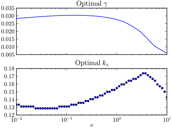
Figure 9: Mean-field growth rate $\gamma$ associated with the optimal $k_{z}$ value as a function of viscosity $\nu$. Other parameters are $\theta_{f}=\pi/4$, $S=1$, $t_{f}=0.1$, $\eta=0.1$, and $\Delta t=0.025$.

Viscous and resistive diffusion both diminish dynamo growth, but they do not suppress it entirely (Figs. 9-10). The growth rate becomes independent of $\nu\rightarrow 0$ for fixed $\eta$, and it becomes independent of $\eta\rightarrow 0$ for fixed $\nu$. The latter indicates that the ESD is a “fast” dynamo with $\gamma\neq 0$ as $\eta\rightarrow 0$ (Roberts and Soward, 1992). At the other extreme, to sustain a dynamo as $\eta\rightarrow\infty$, the value of $k_{z}(\eta)$ must become very small so that resistive decay is not dominant; this is consistent with the limit formulas (82) and (106), where $\gamma(\eta)$ decreases as a power law with exponents of -1 and -5/2, respectively. $\gamma(\nu)$ decreases with $\nu$ for large $\nu$. We can take the $\nu\rightarrow\infty$ limit of (65) for general $\eta$, using the same type of approximation procedure as at the beginning of Sec. 5. The key approximation in this limit is

$$\int^{t}_{0}\,\mathrm{d}{}\lambda\,\int^{\lambda}_{0}\mathrm{d}{}\mu\,G_{\nu}^{\dagger}(\lambda-\mu)G_{\nu}^{\dagger}(t-\mu)\rightarrow\frac{1}{\nu}\,,$$ (108)

with $\mu,\lambda\rightarrow t$ for the arguments of the other integrand factors. The resulting $(L,\nu)$-limit mean-field equation has the same structure as (76) except now the electromotive force curl has a prefactor of $1/\nu$ instead of $1/\eta$. Consequently, $\gamma(\nu)$ must decrease with large $\nu$ as in Fig. 9.

The optimal $\gamma(\theta_{f})$ and $k_{z}(\theta_{f})$ are both largest for intermediate $\theta_{f}$ values (Fig. 11). The limit formulas predict a peak at $\theta_{f}=\pi/2$ and $\gamma=0$ at $\theta_{f}=0,\pi$ ($k_{yf}=0$). However, these limits are based on (76) after $\nu\rightarrow\infty$, which suppresses any effect of shear tilting in the ESD. In the more general case an up-shear orientation ($0<\theta_{f}\pi/2$) is more conducive to dynamo growth. Thus, the Orr effect of phase tilting in shearing waves (Sec. 3.2) augments the dynamo efficiency. This is because, when $\theta_{f}$ is up-shear, the helical forcing factor transiently increases in magnitude as $k_{x}(t)$ decreases between $t=0$ and $t=1/\tan\theta_{f}/S>0$ when $k_{x}(t)$ passes through zero and thereafter becomes increasingly large and negative. This has the effect of transiently augmenting the effective helicity, hence dynamo forcing, compared to a down-shear case where $|k_{x}(t)|$ monotonically increases and the effective helicity only decreases with time. The magnitude of this transient dynamo enhancement is limited by the viscous decay that ensues during the phase tilting toward $k_{x}=0$ (and beyond), consistent with the Orr effect disappearing when $\nu\rightarrow\infty$.

From an ensemble of numerical integrations, we find that the estimate mean value of $\gamma$ is independent of $\theta_{B}$; i.e., the initial conditions of $\boldsymbol{\mathcal{B}}$ are not important for the dynamo apart from the necessity of a seed amplitude in $\boldsymbol{\mathcal{B}}$ to enable the dynamo.

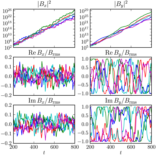
Figure 12: Five ESD realizations in different colors of the mean field component variances, $|\mathcal{B}_{x}|^{2}(t)$ and $|\mathcal{B}_{y}|^{2}(t)$ (top row), and of their real and imaginary parts normalized by $B_{rms}=|\boldsymbol{\mathcal{B}}|(t)$ (bottom two rows). Parameters are $k_{z}=0.14$, $S=1$, $\theta_{f}=\pi/4$, $t_{f}=0.1$, $\nu=0.1$, and $\eta=0.1$. All realizations have the same initial condition $\boldsymbol{\mathcal{B}}(0)$.

The analytic solutions in Sec. 5.1 for the $\eta,\nu\rightarrow\infty$ limit show that the ensemble mean field, ${\cal E}\Big{[}\,\boldsymbol{\mathcal{B}}\,\Big{]}$, has a smaller (but nonzero) dynamo growth rate $\gamma$ than the r.m.s. field for a steady-forcing ensemble as well as a smaller (but undetermined) $\gamma$ for rapidly-varying forcing. Figure 12 illustrates, for a more generic parameter set, how the components of the complex amplitude $\boldsymbol{\mathcal{B}}(t)$ vary substantially both with time and among different realizations, including spontaneous sign reversals on a time scale longer than those directly related to the parameters (i.e., the non-dimensional fluctuation turn-over time of 1, as well as $t_{f}$, $1/S$, $1/\eta$, and $1/\nu$); long-interval reversals also occur for Earth’s magnetic field. This occurs even as the mean magnetic field amplitude inexorably grows, albeit with evident but relatively modest low-frequency and inter-realization variability. It has proved to be computationally difficult to accurately determine the ensemble mean of $\boldsymbol{\mathcal{B}}$ over many random realizations for fixed initial conditions in the general ESD (65). Our computational experience is consistent with the mean field magnitude typically being only a small fraction of the square root of the mean magnetic energy. Thus, the ESD with random small-scale forcing is essentially a random large-scale dynamo.

7 Summary and Prospects

We derive the Elemental Shear Dynamo (ESD) model for a random barotropic force with a single horizontal wavevector in a steady flow with uniform shear in a large domain. It is a quasi-linear theory that is rigorously justified for vanishing magnetic Reynolds number ($1/\eta\rightarrow 0$) and experimentally supported for more general parameters. It robustly exhibits kinematic dynamo behavior as long as the force $\boldsymbol{f}$ has both vertical and horizontal components with finite forcing helicity variance; the vertical wavenumber $k_{z}$ of the initial seed amplitude of the mean magnetic field $\Big{\langle}{\boldsymbol{B}}\Big{\rangle}^{x,y}$ is nonzero but small compared to the horizontal wavenumber of the forcing; and the forcing wavenumber orientation is not shear-normal (i.e., $k_{yf}\neq 0$). When these conditions are satisfied, the dynamo growth rate is larger when $S$ is larger, the resistivity $\eta$ and viscosity $\nu$ are smaller, the forcing correlation time $t_{f}$ is larger, and the forcing wavenumber $\theta_{f}$ is in an upshear direction. The ensemble-mean of the energy of the horizontally averaged magnetic field grows as a dynamo, but the energy of the ensemble-mean magnetic field is much smaller. Reversals in $\Big{\langle}{\boldsymbol{B}}\Big{\rangle}^{x,y}(t)$ are common over time intervals long compared to $t_{f}$. Because the growth-rate curves have broad maxima in both parameters and fluctuation wavenumbers (Sec. 6), we expect dynamo action with a broad spectrum in $\boldsymbol{k}_{f}$ and $k_{z}$, consistent with the quasi-linear superposition principle (69).

The ESD ingredients of small-scale velocity fluctuations and large-scale shear are generic across the universe, so its dynamo process is likely to be relevant to the widespread existence of large-scale magnetic fields. Of course, the simple spatial symmetries assumed in the ESD model are a strong idealization of natural flows, and the ESD is not a general MHD model because of its quasi-linearity assumptions. Investigation of more complex situations is needed to determine the realm of relevance for the ESD behavior shown here, especially in turbulent flows with intrinsic variability and large Reynolds number.

Acknowledgments: This work benefited greatly from extensive discussions with Tobias Heinemann, who also helped with some of the calculations and figures, and with Alexander Schekochihin, who has led our inquiry into the shear dynamo. I also appreciate a long and fruitful partnership with Steven Cowley on dynamo behaviors, first at small scales and now at large. This paper is a fruit of unsponsored research.

Appendix A Derivation of $\boldsymbol{F}_{\mathcal{B}}$ in (60)

This appendix fills in steps between the formal expression for the curl of the mean electromotive force (59) and its particular expression in the ESD (60). Here we retain the convention that all vectors are horizontal.

To provide a more compact notation, we rewrite the vertical phase factor coefficient for the fluctuation field (55) as

$$\boldsymbol{b}(x,y,t) =\int^{t}_{0}\,\mathrm{d}{}\lambda\,\int^{\lambda}_{0}\mathrm{d}{}\mu\ \Bigl{[}\ \boldsymbol{b}_{+}(t,\lambda,\mu)\,e^{\mathrm{i}\phi(\mu)}+\ \boldsymbol{b}_{-}(t,\lambda,\mu)\,e^{-\mathrm{i}\phi(\mu)}\ \Bigr{]}\,,$$ (109)

where

$$\boldsymbol{b}_{+} =\frac{1}{2}\,G_{\eta}(t-\mu,\lambda-\mu)G_{\nu}(\lambda-\mu)\ \Bigl{[}\ k_{z}\Bigl{(}\,-\,\mathrm{i}\hat{f}_{z}(\mu)\mathsfbi{S}(t-\lambda)\cdot\boldsymbol{\mathcal{B}}(\lambda)\,\Bigr{)}$$

$$\ +\,\frac{\boldsymbol{e}_{z}\times\boldsymbol{k}(t-\mu)}{k^{2}(\lambda-\mu)}\,\Bigl{(}\,\hat{o}_{z}(\mu)\,(\boldsymbol{k}(\lambda-\mu)\cdot\boldsymbol{\mathcal{B}}(\lambda))\,\Bigr{)}\ \Bigr{]}$$

$$\boldsymbol{b}_{-} =\frac{1}{2}\,G_{\eta}(t-\mu,\lambda-\mu)G_{\nu}(\lambda-\mu)\ \Bigl{[}\ k_{z}\Bigl{(}\,-\,\mathrm{i}\hat{f}_{z}^{\ast}(\mu)\mathsfbi{S}(t-\lambda)\cdot\boldsymbol{\mathcal{B}}(\lambda)\,\Bigr{)}$$

$$\ +\,\frac{\boldsymbol{e}_{z}\times\boldsymbol{k}(t-\mu)}{k^{2}(\lambda-\mu)}\,\Bigl{(}\,\hat{o}_{z}^{\ast}(\mu)\,(\boldsymbol{k}(\lambda-\mu)\cdot\boldsymbol{\mathcal{B}}(\lambda))\,\Bigr{)}\ \Bigr{]}\,.$$ (110)

We evaluate the three terms for $\Big{\langle}{\,\boldsymbol{F}_{\mathcal{B}}\,}\Big{\rangle}^{x,y}$ in (59) for each of the terms in $\boldsymbol{b}_{+}$ and $\boldsymbol{b}_{-}$. To do so involves the spatial average of products of factors with exponential phase functions, $\mathrm{i}(\,\pm\,\phi+k_{z}z)$. Employing (40) we will make use of the general identities,

$$\Big{\langle}{\,\mathrm{Re}\left\{A_{1}(\rho)\,e^{\mathrm{i}\phi(\rho)}\right\}\ \mathrm{Re}\left\{A_{2}(\mu)\,e^{\mathrm{i}\phi(\mu)}e^{\mathrm{i}k_{z}z}\right\}\,}\Big{\rangle}^{x,y}=\frac{C_{L}}{2}\,\delta(\rho-\mu)\,\mathrm{Re}\left\{A_{1}^{\ast}A_{2}e^{\mathrm{i}k_{z}z}\right\}$$

$$\Big{\langle}{\,\mathrm{Re}\left\{A_{1}(\rho)\,e^{\mathrm{i}\phi(\rho)}\right\}\ \mathrm{Re}\left\{A_{2}(\mu)\,e^{-\mathrm{i}\phi(\mu)}e^{\mathrm{i}k_{z}z}\right\}\,}\Big{\rangle}^{x,y}=\frac{C_{L}}{2}\,\delta(\rho-\mu)\,\mathrm{Re}\left\{A_{1}A_{2}e^{\mathrm{i}k_{z}z}\right\}\,.$$ (111)

The first term in (59) is evaluated as follows:

$$-\,\Big{\langle}\,(\boldsymbol{u}\cdot{\nabla})\boldsymbol{b}^{\prime}\,\Big{\rangle}^{x,y}$$

$$\quad=-\,\Big{\langle}\,\left(\,\int_{0}^{t}\,\mathrm{d}{}\rho\,G_{\nu}(t-\rho)\,\left(\frac{-\,\boldsymbol{e}_{z}\times\boldsymbol{k}(t-\rho)}{k^{2}(t-\rho)}\right)\,\mathrm{Re}\left\{\,\mathrm{i}\hat{o}_{z}(\rho)\,e^{\mathrm{i}\phi(\rho)}\,\right\}\cdot\boldsymbol{k}(t-\mu)\,\right)\$$

$$\qquad\qquad\qquad\int^{t}_{0}\,\mathrm{d}{}\lambda\,\int^{\lambda}_{0}\mathrm{d}{}\mu\ \Bigl{[}\ \mathrm{Re}\left\{\mathrm{i}\boldsymbol{b}_{+}(t,\lambda,\mu)\,e^{\mathrm{i}\phi(\mu)}e^{\mathrm{i}k_{z}z}\right\}$$

$$\qquad\qquad\qquad\qquad+\ \mathrm{Re}\left\{-\mathrm{i}\boldsymbol{b}_{-}(t,\lambda,\mu)\,e^{-\mathrm{i}\phi(\mu)}e^{\mathrm{i}k_{z}z}\right\}\ \Bigr{]}\,\Big{\rangle}^{x,y}$$

$$\quad=\ \frac{C_{L}}{2}\,\int^{t}_{0}\,\mathrm{d}{}\lambda\,\int^{\lambda}_{0}\mathrm{d}{}\mu\,G_{\nu}(t-\mu)\,\left(\frac{\boldsymbol{e}_{z}\times\boldsymbol{k}(t-\mu)\cdot\boldsymbol{k}(t-\mu)}{k^{2}(t-\rho)}\right)$$

$$\qquad\qquad\qquad\qquad\mathrm{Re}\left\{\,\left(\hat{o}_{z}^{\ast}\boldsymbol{b}_{+}+\hat{o}_{z}\boldsymbol{b}_{-}\right)\,e^{\mathrm{i}k_{z}z}\,\right\}$$

$$\quad=\ 0\,.$$ (112)

The formula (111) is used to obtain the middle right-hand side, and the final result comes from the identify, $\boldsymbol{e}_{z}\times\boldsymbol{a}\cdot\boldsymbol{a}=0$.

The second term in (59) is evaluated as follows:

$$-\,\Big{\langle}\,(u_{z}\partial_{z})\boldsymbol{b}^{\prime}\,\Big{\rangle}^{x,y}$$

$$\quad=-\,\Big{\langle}\,\left(\,\int_{0}^{t}\,\mathrm{d}{}\rho\,G_{\nu}(t-\rho)\,\mathrm{Re}\left\{\,\hat{f}_{z}(\rho)\,e^{\mathrm{i}\phi(\rho)}\,\right\}\,k_{z}\,\right)\$$

$$\qquad\qquad\int^{t}_{0}\,\mathrm{d}{}\lambda\,\int^{\lambda}_{0}\mathrm{d}{}\mu\ \Bigl{[}\ \mathrm{Re}\left\{\mathrm{i}\boldsymbol{b}_{+}(t,\lambda,\mu)\,e^{\mathrm{i}\phi(\mu)}e^{\mathrm{i}k_{z}z}\right\}$$

$$\qquad\qquad\qquad\qquad+\ \mathrm{Re}\left\{\mathrm{i}\boldsymbol{b}_{-}(t,\lambda,\mu)\,e^{-\mathrm{i}\phi(\mu)}e^{\mathrm{i}k_{z}z}\right\}\ \Bigr{]}\,\Big{\rangle}^{x,y}$$

$$\quad=-\,\frac{C_{L}}{2}\,\int^{t}_{0}\,\mathrm{d}{}\lambda\,\int^{\lambda}_{0}\mathrm{d}{}\mu\,G_{\nu}(t-\mu)k_{z}\,\mathrm{Re}\left\{\,\mathrm{i}\left(\hat{f}_{z}^{\ast}\boldsymbol{b}_{+}+\hat{f}_{z}\boldsymbol{b}_{-}\right)\,e^{\mathrm{i}k_{z}z}\,\right\}$$

$$\quad=-\,\frac{C_{L}}{2}\,\int^{t}_{0}\,\mathrm{d}{}\lambda\,\int^{\lambda}_{0}\mathrm{d}{}\mu\,G_{\eta}(t-\mu,\lambda-\mu)G_{\nu}(\lambda-\mu)G_{\nu}(t-\mu)\,$$

$$\qquad\qquad\qquad\Bigl{[}\ |\hat{f}_{z}|^{2}(\mu)\,k_{z}^{2}\,\mathrm{Re}\left\{\mathsfbi{S}(t-\lambda)\cdot\boldsymbol{\mathcal{B}}(\lambda)e^{\mathrm{i}k_{z}z}\right\}$$

$$\ +\,\mathrm{Re}\left\{\hat{f}_{z}^{\ast}(\mu)\hat{o}_{z}(\mu)\right\}\,k_{z}\,\boldsymbol{e}_{z}\times\boldsymbol{k}(t-\mu)\,\Bigl{(}\,\frac{\boldsymbol{k}(\lambda-\mu)}{k^{2}(\lambda-\mu)}\cdot\mathrm{Re}\left\{\mathrm{i}\boldsymbol{\mathcal{B}}(\lambda)e^{\mathrm{i}k_{z}z}\right\}\,\Bigr{)}\ \Bigr{]}\,.$$ (113)

The formula (111) is used to obtain the second right-hand side, and (110) is substituted to obtain the final result, which agrees with the first and second terms in (60).

The final term in (59) is evaluated as follows:

$$\Big{\langle}\,(\boldsymbol{b}^{\prime}\cdot{\nabla})\boldsymbol{u}\,\Big{\rangle}^{x,y}$$

$$\quad=\,\Big{\langle}\,\int^{t}_{0}\,\mathrm{d}{}\lambda\,\int^{\lambda}_{0}\mathrm{d}{}\mu\,\int_{0}^{t}\,\mathrm{d}{}\rho\,G_{\nu}(t-\rho)\,\left(\frac{-\,\boldsymbol{e}_{z}\times\boldsymbol{k}(t-\rho)}{k^{2}(t-\rho)}\right)\,\mathrm{Re}\left\{\,\mathrm{i}\,\mathrm{i}\,\hat{o}_{z}(\rho)\,e^{\mathrm{i}\phi(\rho)}\,\right\}$$

$$\qquad\qquad\qquad\Bigl{(}\,\boldsymbol{k}(t-\rho)\ \cdot\ \Bigl{[}\ \mathrm{Re}\left\{\boldsymbol{b}_{+}(t,\lambda,\mu)\,e^{\mathrm{i}\phi(\mu)}e^{\mathrm{i}k_{z}z}\right\}$$

$$\qquad\qquad\qquad\qquad\qquad\qquad+\ \mathrm{Re}\left\{\boldsymbol{b}_{-}(t,\lambda,\mu)\,e^{-\mathrm{i}\phi(\mu)}e^{\mathrm{i}k_{z}z}\right\}\ \Bigr{]}\,\Bigr{)}\,\Big{\rangle}^{x,y}$$

$$\quad=\ \frac{C_{L}}{2}\,\int^{t}_{0}\,\mathrm{d}{}\lambda\,\int^{\lambda}_{0}\mathrm{d}{}\mu\,G_{\nu}(t-\mu)\,\frac{\boldsymbol{e}_{z}\times\boldsymbol{k}(t-\mu)}{k^{2}(t-\mu)}\,$$

$$\qquad\qquad\qquad\Bigl{(}\,\boldsymbol{k}(t-\mu)\ \cdot\ \mathrm{Re}\left\{\,\left(\hat{o}_{z}^{\ast}\boldsymbol{b}_{+}+\hat{o}_{z}\boldsymbol{b}_{-}\right)\,e^{\mathrm{i}k_{z}z}\,\right\}\,\Bigr{)}$$

$$\quad=-\,\frac{C_{L}}{2}\,\int^{t}_{0}\,\mathrm{d}{}\lambda\,\int^{\lambda}_{0}\mathrm{d}{}\mu\,G_{\eta}(t-\mu,\lambda-\mu)G_{\nu}(\lambda-\mu)G_{\nu}(t-\mu)\,\frac{\boldsymbol{e}_{z}\times\boldsymbol{k}(t-\mu)}{k^{2}(t-\mu)}\,$$

$$\qquad\qquad\qquad k_{z}\mathrm{Re}\left\{\hat{f}_{z}^{\ast}\hat{o}_{z}\right\}\,\Bigl{(}\,\boldsymbol{k}(t-\mu)\ \cdot\mathrm{Re}\left\{\,\mathrm{i}\mathsfbi{S}(t-\lambda)\cdot\boldsymbol{\mathcal{B}}(\lambda)e^{\mathrm{i}k_{z}z}\,\right\}\,\Bigr{)}\,.$$ (114)

Again, (111) is used to obtain the second right-hand side, and (110) is substituted to obtain the final result, which agrees with the third term in (60). In this substitution, the terms in $\boldsymbol{b}_{\pm}\ \propto\ \hat{o}_{z},\ \hat{o}_{z}^{\ast}$ do not survive because they yield a factor, $\boldsymbol{e}_{z}\times\boldsymbol{k}(t-\mu)\cdot\boldsymbol{k}(t-\mu)=0$.

This completes the derivation of (60).

Appendix B Computational Solution of (65)

The ESD solutions in Sec. 4.3 are obtained by numerical integration of the integro-differential equation system (65). This system is potentially expensive to solve because of the two time integrals, requiring $O(T^{3})$ operations to integrate to time $T$. We convert this to an $O(T)$ system (formally comparable to the size an ODE integration, albeit with a much larger coefficient for $T$) by limiting the integration range to fixed intervals, $t-\tau\leq\lambda,\leq t$ and $t-\tau\leq\mu\leq\lambda$, once $t>\tau$; for smaller $t$ values, the integrations start from $\lambda=\mu=0$. A sufficient motivation for this approximation is that the two viscous decay factors (32) become vanishingly small for large values of its arguments $t-\mu$ and $\lambda-\mu$ in (65). For a given $\nu$ value, we determine $\tau$ by the requirement that $G_{\nu}(\tau)\leq\hat{\epsilon}\ll 1$. In practice we typically choose $\hat{\epsilon}=10^{-7}$ and make sure that the results do not change significantly if we further decrease the value of $\hat{\epsilon}$.

The domain of integration is a triangle in $(\lambda,\mu)$-space. Because of this, the forcing functions $\mathcal{F}(\mu)$ and $\mathcal{H}(\mu)$ only need to be retained in memory for the range $t-\tau\leq\mu\leq{}t$ to evaluate $\widetilde{\boldsymbol{\dot{\mathcal{B}}}}(t)$ and advance $\widetilde{\boldsymbol{\mathcal{B}}}(t)$ in time. With the restricted integration intervals, the mean field equation (65) is

$$\boldsymbol{\dot{\widetilde{\mathcal{B}}}}(t)=S\widetilde{\mathcal{B}}_{x}(t)\,\boldsymbol{e}_{y}+\int_{t-\tau}^{t}\!\mathrm{d}\lambda\int_{t-\tau}^{\lambda}\!\mathrm{d}\mu\,\Bigl{[}\mathcal{F}(\mu)\mathcal{P}(t-\mu,\lambda-\mu)+\mathrm{i}\mathcal{H}(\mu)\mathcal{Q}(t-\mu,\lambda-\mu)\Bigr{]}\cdot\widetilde{\boldsymbol{\mathcal{B}}}(\lambda)\,,$$ (115)

where we have introduced the second-order matrices,

$$\mathcal{P}(t_{1},t_{2})=-k_{z}^{2}G_{\eta}(t_{1},t_{2})G_{\nu}(t_{1})G_{\nu}(t_{2})\mathcal{S}(t_{1}-t_{2})$$ (116)

and

$$\mathcal{Q}(t_{1},t_{2})=-k_{z}G_{\eta}(t_{1},t_{2})G_{\nu}(t_{1})G_{\nu}(t_{2})\Bigl{[}k^{-2}(t_{1})+k^{-2}(t_{2})\Bigr{]}(\boldsymbol{e}_{z}\times\boldsymbol{k}(t_{1}))\,\boldsymbol{k}(t_{2})\,.$$ (117)

We may convert the double time integral in (115) to a double time integral ‘into the past’ via the substitutions $\lambda^{\prime}=t-\lambda$ and $\mu^{\prime}=t-\mu$, giving

$$\boldsymbol{\dot{\widetilde{\mathcal{B}}}}(t)=S\widetilde{\mathcal{B}}_{x}(t)\boldsymbol{e}_{y}+\int_{0}^{\tau}\!\mathrm{d}\lambda^{\prime}\int_{\lambda^{\prime}}^{\tau}\!\mathrm{d}\mu^{\prime}\,\Bigl{[}\mathcal{F}(t-\mu^{\prime})\mathcal{P}(\mu^{\prime},\mu^{\prime}-\lambda^{\prime})+\mathrm{i}\mathcal{H}(t-\mu^{\prime})\mathcal{Q}(\mu^{\prime},\mu^{\prime}-\lambda^{\prime})\Bigr{]}\cdot\widetilde{\boldsymbol{\mathcal{B}}}(t-\lambda^{\prime})\,.$$ (118)

Note that, because $0\leq\lambda^{\prime}\leq\mu^{\prime}\leq\tau$, the matrices (116) and (117) can be evaluated once and for all in the ranges $0\leq{}t\leq\tau$ and $0\leq\lambda\leq\tau$ at the beginning of the simulation.

To discretize (118) in time, we write this equation as a system of one integro-differential and one integral equation, viz.,

$$\boldsymbol{\dot{\widetilde{\mathcal{B}}}}(t)=S\widetilde{\mathcal{B}}_{x}(t)\boldsymbol{e}_{y}-\int_{0}^{\tau}\!\mathrm{d}\lambda\,\mathcal{G}(t,\lambda)\cdot\widetilde{\boldsymbol{\mathcal{B}}}(t-\lambda)$$ (119)

and

$$\mathcal{G}(t,\lambda)=\int_{\lambda}^{\tau}\!\mathrm{d}\mu\Bigl{[}\mathcal{F}(t-\mu)\mathcal{P}(\mu,\mu-\lambda)+\mathrm{i}\mathcal{H}(t-\mu)\mathcal{Q}(\mu,\mu-\lambda)\Bigr{]}\,,$$ (120)

where we have now dropped the primes from $\lambda$ and $\mu$. Using the trapezoidal rule, a second-order accurate representation of (119) is given by

$$\frac{\boldsymbol{\mathcal{B}}^{n+1}-\mathcal{S}(\Delta t)\cdot\boldsymbol{\mathcal{B}}^{n}}{\Delta t}=\mathcal{S}(\Delta t)\cdot\left(\frac{\Delta t}{4}\mathcal{G}^{n,0}\cdot\boldsymbol{\mathcal{B}}^{n}+\frac{\Delta t}{2}\sum_{m=1}^{K-1}\mathcal{G}^{n,m}\cdot\boldsymbol{\mathcal{B}}^{n-m}\right)\\ +\left(\frac{\Delta t}{4}\mathcal{G}^{n+1,0}\cdot\boldsymbol{\mathcal{B}}^{n+1}+\frac{\Delta t}{2}\sum_{m=1}^{K-1}\mathcal{G}^{n+1,m}\cdot\boldsymbol{\mathcal{B}}^{n+1-m}\right)\,,$$ (121)

where $\widetilde{\boldsymbol{\mathcal{B}}}^{n}=\widetilde{\boldsymbol{\mathcal{B}}}(n\Delta{}t)$ and $\mathcal{G}^{n,m}=\mathcal{G}(n\Delta{}t,m\Delta{}t)$; we have anticipated (122b) below. The integer $K$ is defined through the relation $\tau=K\Delta{}t$. The matrix factor $\mathcal{S}(\Delta{}t)$ arises from treating the shear stretching term exactly. Because (121) is linear, it may be easily solved for $\widetilde{\boldsymbol{\mathcal{B}}}^{n+1}$ provided the matrix $\mathcal{G}^{n+1,0}$ can be inverted. To compute $\mathcal{G}^{n,m}$, we again use the trapezoidal rule to obtain

$$\mathcal{G}^{n,m} =\frac{\Delta t}{2}\left(\mathcal{F}^{n-m}\mathcal{P}^{m,0}+\mathrm{i}\mathcal{H}^{n-m}\mathcal{Q}^{m,0}\right)$$

$$+\Delta t\sum_{l=m+1}^{K-1}\left(\mathcal{F}^{n-l}\mathcal{P}^{l,l-m}+\mathrm{i}\mathcal{H}^{n-l}\mathcal{Q}^{l,l-m}\right)$$

$$+\frac{\Delta t}{2}\left(\mathcal{F}^{n-K}\mathcal{P}^{K,K-m}+\mathrm{i}\mathcal{H}^{n-K}\mathcal{Q}^{K,K-m}\right)$$ (122a)

$$\mathcal{G}^{n,K} =0\,.$$ (122b)

References

- Brandenburg & Subramanian (2005) Brandenburg, A. & Subramanian, K. 2005 Astrophysical magnetic fields and nonlinear dynamo theory. Physics Reports 417, 1–209.
- Heinemann et al. (2011a) Heinemann, T., McWilliams, J. C. & Schekochihin, A. 2011a Magnetic field generation by randomly forced shearing waves. Submitted to Phys. Rev. Lett.
- Heinemann et al. (2011b) Heinemann, T., McWilliams, J. C. & Schekochihin, A. 2011b The shear dynamo in dimensions. In preparation.
- Krause & Radler (1980) Krause, F. & Radler, K. H. 1980 Mean-Field Magnetohydrodynamics and Dynamo Theory. Pergamon Press.
- Kulsrud (2010) Kulsrud, R. H. 2010 The origin of our galatic magnetic field. Astron. Nachr. 331, 22–26.
- Moffatt (1978) Moffatt, H. K. 1978 Magnetic Field Generation in Electrically Conducting Fluids. Cambridge University Press.
- Parker (1971) Parker, E. N. 1971 The generation of magnetic fields in astrophysical bodies. II. The galactic field. Ap. J. 163, 255–278.
- Roberts & Soward (1992) Roberts, P. H. & Soward, A. M. 1992 Dynamo theory. Ann. Rev. Fluid Mech. 24, 459–512.
- Silant’ev (2000) Silant’ev, N.A. 2000 Magnetic dyanmo due to turbulent helicity fluctuations. Astron. Astrophys. 364, 339–347.
- Sridhar & Subramanian (2009) Sridhar, S. & Subramanian, K. 2009 Nonperturbative quasi-linear approach to the shear dynamo problem. Phys. Rev. E 80, 0066315.
- van Kampen (2007) van Kampen, N. 2007 Stochastic Processes in Physics and Chemistry. Elsevier, 3rd edition.
- Vishniac & Brandenburg (1997) Vishniac, E. & Brandenburg, A. 1997 An incoherent dynamo in accretion disks. Ap. J. 475, 263–274.
- Yousef et al. (2008a) Yousef, T. A., Heinemann, T., Schekochinin, A. A., Kleeorin, N., Rogachevskii, I., Cowley, S. C. & McWilliams, J. C. 2008a Numerical experiments on dynamo action in sheared and rotating turbulence. Astron. Nachr. 329, 737–749.
- Yousef et al. (2008b) Yousef, T. A., Heinemann, T., Schekochinin, A. A., Kleeorin, N., Rogachevskii, I., Iskakov, A. B., Cowley, S. C. & McWilliams, J. C. 2008b Generation of magnetic field by combined action of turbulence and shear. Phys. Rev. Lett. 100, 184501.