UNIVERSITY OF SCIENCE AND TECHNOLOGY OF CHINA
Heifei, CHINA




Relativistic fluid dynamics in heavy ion collisions

Dedicated to my dear family

Abstract

Quantum Chromodynamics (QCD) is the fundamental theory for strong interaction, one of the four forces in nature. Different from electromagnetic interaction, due to its non-Abelian color symmetry, the QCD has the property of asymptotic freedom at large momentum transfer, while remains strongly coupled at low energies. This property leads to color confinement, i.e. there are no free quarks and gluons carrying color degree of freedom, and quarks and gluons are confined inside hadrons. In 1974-75, Lee and Collins-Perry suggested that the deconfinement can be reached through the ultra-relativistic heavy ion collisions, where the vacuum can be excited to a new state of matter or a quark gluon plasma. In the Relativistic Heavy Ion Collider (RHIC) at Brookhaven National Lab (BNL), the gold nuclei are accelerated and collide head-to-head at the center-of-mass energy of 200 GeV per nucleon. After the collisions, the huge amount of energy is deposited in the central rapidity region to excite vacuum and produce many quarks and gluons. In very short time, these quarks and gluons collide to each other and the fireball reaches the local thermal equilibrium, and a quark-gluon-plasma (QGP) is then formed. After expansion and cooling, the temperature drops substantially and the quarks recombine into hadrons which are finally observed in detectors. The collective flows such as radial and elliptic flows are observed at RHIC and can be well described by ideal fluid dynamics. Further study of the elliptic flow using dissipative fluid dynamics gives very low values of the ratio of shear viscosity to entropy density, close to the lower bound $1/4\pi$ by AdS/CFT correspondence. This is one of the most surprising observation at RHIC: the QGP is strongly coupled or a nearly perfect liquid instead of a gas-like weakly coupled system by convention. The relativistic fluid dynamics provides a useful tool to bridge the gap between the initial state of quarks and gluons and the experimental data. Pushed by heavy ion collision experiments, the theory of relativistic fluid dynamics also has a lot of new development in recent years. This thesis is about the study of three important issues in the theory of relativistic fluid dynamics: the stability of dissipative fluid dynamics, the AdS/CFT application to shear viscosity in a Bjorken expanding fluid, and a consistent description of kinetic equation with triangle anomaly.

Hydrodynamics is a long-wavelength effective theory for many particle systems. The basic hydrodynamic equation consists of conservation equations of energy-momentum and charge numbers. One can carry out gradient expansion for energy-momentum tensor and charge currents, or equivalently expansion in powers of the Knudsen number. The Knudsen number is defined as the ratio of the macroscopic length scale (hydrodynamic wave-length) to the microscopic one (mean free path). When the macroscopic length scale is much larger than the microscopic one, the fluid dynamics is a good effective theory. In expansion, the zeroth order corresponds to the ideal fluid. The first order gives the Navier-Stokes equations with dissipative terms like shear and bulk viscous terms. There are a lot of candidates for the second order theory. We focus on the widely used Israel-Stewart (IS) theory including the simplified and complete version. The simplified version can be obtained by correspondence to the macroscopic phenomena. To derive the complete version the kinetic theory or the Boltzmann equation is necessary. In this thesis, we will give the details as how to obtain the complete version. The connection between the transport coefficients in the first and the second order theories will be demonstrated.

In the first order theory, causality is violated since it takes no time for a system in a non-equilibrium state to reach equilibrium, i.e. the propagating speed of the signal is arbitrarily large. In the second order theory, due to finite relaxation time introduced, it takes finite time for the system to reach equilibrium. The propagating speed of the signal is limited. Therefore the second order theory is necessary for causality. However the causality cannot be guaranteed for all parameters. The constraints for parameters are then given. We also point out that the causality and the stability are inter-correlated. Relativity requires that the signal propagate in light-cones. An acausal propagating modes must be forbidden by instability or singularity. The connection between causality and stability is also discussed. For convenience we work in a general boost frame. It is found that a causal system must be stable, but an acausal system in the boost frame at high speed must be unstable.

The transport coefficients can be determined in kinetic theory. There are two main techniques to compute the transport coefficients. One is to employ the Boltzmann equation, the other is to use the Kubo formula in field theory. We will firstly discuss about derivation of the shear viscosity via variational method in the Boltzmann equation. Secondly, after a short review of Kubo formula, we will compute the shear viscosity via AdS/CFT duality.

Different from the work of Policastro, Son and Starinets (PSS), we focus on strongly coupled QGP (sQGP) with the radial expansion and Bjorken boost invariance. The information of the sQGP is encoded on the boundary of AdS space via the holographic renormalization. Solving the Einstein equation with the boundary condition given by the stress tensor yields the metric of the AdS space. In this case, the metric is Bjorken boost invariant and has the radial flow. The evolution of the shear viscosity as a function of proper time can be obtained via the Kubo formula for the retarded Green function given by the AdS/CFT duality. It is found that the ratio of the shear viscosity to entropy density is consistent with PSS.

As another application of AdS/CFT duality, we investigate the property of baryons in sQGP in a Wilson-loops-like model. The quarks located at the boundary of AdS space are connected to a probe D5 brane by superstrings. By studying the configurations of baryons with different spins, the screening length of baryons can be obtained as a function of spin and temperature. We also study the relationship between the angular momentum and energy for different kinds of baryons, which shows the Regge-like behavior, i.e. the total angular momentum is proportional to the energy squared.

As the last topic, we investigate the fluid dynamics with quantum triangle anomalies. Generally the relativistic fluid dynamics does not allow the vorticity due to parity conservation. Recently it is pointed out that the vorticity has to be introduced to relativistic fluid dynamics with anomalies to satisfy the second law of thermodynamics. These new terms are also relevant to the Chiral Magnetic Effect (CME) or Chiral Vorticity Effect (CVE). Such terms can be derived from the kinetic approach. The coefficients of the vorticity in the case of right-handed quarks (or left-handed anti-quarks) and quarks-antiquarks of mixed chirality are evaluated.

Chapter 1 Introduction

1.1 Quantum Chromodynamics and deconfinement phase transition

1.1.1 Asymptotic freedom

Quantum Chromodynamics (QCD) is a gauge theory for the strong interaction which is one of the four fundamental interactions in the nature. In contrast to photons in Quantum Electrodynamics (QED), the interaction for gluons are complicated because of non-Abelian $SU(3)$ color symmetry. The coupling constant $\alpha_{s}$ of renormalized QCD in one-loop approximation is given by

$$\alpha_{s}(Q^{2})=\frac{\alpha_{s}(M^{2})}{1+b_{0}\frac{\alpha_{s}(M^{2})}{2\pi}\ln(Q^{2}/M^{2})}\;,$$ (1.1)

where $Q$ is the momentum transfer scale, $M$ is the energy scale and $b_{0}=\frac{33-2N_{f}}{3}$ is the first coefficient of $\beta$-function given by the renormalization group equation with the quark flavor $N_{f}$. Here $\alpha_{s}(M^{2})$ can be chosen as $\alpha_{s}(M_{Z}^{2})$ at Z-boson mass $M_{z}$ [1, 2]

$$\alpha_{s}(M_{Z}^{2})=0.1184\pm 0.0007\;.$$ (1.2)

The data for $\alpha_{s}(Q^{2})$ [2] are shown in Fig.1.1. Equation (1.1) indicates that the coupling constant decreases with the energy scale $Q$. This property is the called asymptotic freedom [3, 4]. The interaction for quarks and gluons will be strong in the low energy scale which leads to confinement, i.e. quarks are limited inside hadrons in vacuum or the ground state.

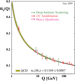
Figure 1.1: Measurements of $\alpha_{s}$ as a function of the momentum transfer $Q$ [2].

In the early 1970s Lee and Collins et al. [5, 6] proposed that the deconfinement can be reached through the ultra-relativistic heavy ion collisions. According to the calculations from lattice QCD, the confinement/deconfinement phase transition will take place at temperature of about 170 MeV in three flavor case [7] as shown in Fig. 1.2.

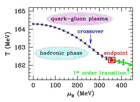
Figure 1.2: Phase diagram of QCD from the lattice calculations with non-zero chemical potential [8].

1.1.2 Experiments for high energy heavy ion collisions

1.1.2.1 RHIC experiments

Relativistic Heavy Ion Collider (RHIC) at Brookhaven National Laboratory (BNL) has been running since 2000. Two beams of nuclei (Au or Cu) are accelerated to collide with the center-of-mass energy of 200 GeV/nucleon or 62.4 GeV/nucleon. After the most part of nuclei pass through each other, the huge amount of energy is deposited in the central rapidity region, and thus excites the quarks and gluons from the vacuum. These quarks and gluons form an expanding fireball, and reach the local thermal equilibrium within a extremely short time of $1\sim 2fm/c$. It is believed that new state of matter, the quark-gluon-plasma (QGP) has been formed [9, 10]. The QGP expands and cools down with it freezes out at some critical temperature, below which the quarks recombine into hadrons observed by the detectors.

The collective flows such as radial and elliptic flows are observed at RHIC and can be well described by ideal fluid dynamics. In non-central collisions, the anisotropic momentum leads to the gradient of pressure. This effect can be detected by analysis of the final particle spectrum in momentum space. The Fourier transformation for the particle spectrum in terms of particle azimuthal angle $\phi$ with respect to the reaction plane $\psi_{r}$ gives

$$E\frac{d^{3}N}{dp^{3}}=\frac{d^{2}N}{2\pi p_{T}dp_{T}dy}\left\{1+\sum_{n=1}^{\infty}2v_{n}\cos[n(\phi-\psi_{r})]\right\}\;.$$ (1.3)

where the second coefficient $v_{2}$ is the anisotropy parameter, which is also called elliptic flow. The data from RHIC have delivered a surprising result that elliptic flow $v_{2}$ is very large [11, 12, 13, 14] and compatible with the numerical simulations of ideal fluid dynamics [15, 16, 17, 18], see Fig. 1.3. This indicates that the QGP is strongly coupled in contrast to the assumption that QGP is a weakly coupled system.

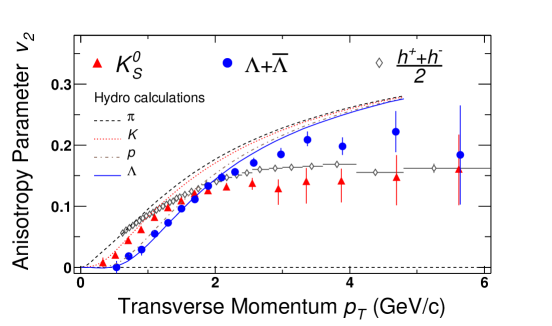
Figure 1.3: The elliptic flow measured at RHIC with prediction given by hydrodynamics [11].

Further study for QGP gives very low values of the ratio of shear viscosity to entropy density $\eta/s\sim 0.1$[19, 20] close to the theoretical lower bound given by AdS/CFT duality [21], see Fig. 1.4. For a weakly coupled system with well-defined quasi-particles, the ratio $\eta/s$ is very large [22, 23]. For the system with strong couplings, the lower bound from the AdS/CFT duality is $1/(4\pi)$ [24, 25] in the comparison with the $1/12$ evaluated from the uncertainty principle [26]. Therefore, the fact that $\eta/s$ of QGP is close to the lower bound is one piece of most convincing evidence that QGP is strongly coupled. The calculations for the ratio are shown in Chap. 4 for a weakly coupled system and Chap. 5 for a strongly coupled system.

There are a lot of other interesting and important phenomena at RHIC experiment, e.g. the jet quenching, parton energy loss, heavy quark production, etc. (see e.g. Ref. [15, 27, 28, 29, 30, 31, 32] for reviews). Those phenomena will also be mentioned in the relevant sections.

1.1.2.2 LHC experiments

The main goal of the Large Hadron Collider (LHC) experiments at European Organization for Nuclear Research (CERN) is to discover the Higgs bosons, supersymmetic particles and other new physics. There are three major experiments: A Toroidal LHC Apparatus (ATLAS), Compact Muon Solenoid (CMS), and A Large Ion Collider Experiment (ALICE). The purpose of ATLAS and CMS experiments is to hunt for Higgs boson and new physics, while the ALICE experiment is to pin down and study the QGP.

In the CMS experiment, the two-particle angular correlations for charged particles in the proton-proton (pp) collisions at center-of-mass energies of $0.9$, $2.36$, and $7$ GeV are measured. A long-range, near-side feature in two-particle correlation functions have been observed in pp collisions for the first time [33]. A ridge-like structure is observed in the two-dimensional correlation function for particle pairs with intermediate transverse momentum of $1-3$GeV$/c$, $2.0<\left|\Delta\eta\right|<4.8$ and $\Delta\phi\approx 0$ with $\eta$ the pseudorapidity and $\phi$ the azimuthal angle. Some authors [34, 35] thought that this discovery might imply the QGP has also been formed in the pp collisions. The collective flow has also been analyzed [36, 37]. The relativistic fluid dynamics may become a powerful tool to investigate the new phenomena in the ultra high energy pp collisions at LHC.

The first Pb-Pb collision at center-of-mass energy of 2.7 TeV was realized at LHC in November 2010 [38, 39]. The ALICE experiment is aimed to search for QGP at 2 to 3 times higher temperatures than RHIC. Since the collisional energy at LHC is one magnitude larger than at RHIC, the perturbative QCD (pQCD) is expected to work much better than at RHIC. The semi-classical Boltzmann equation with the collision terms given by the pQCD is a good tool to describe non-equilibrium dynamics of the QGO formed in heavy ion collisions at LHC.

1.2 Relativistic fluid dynamics and kinetic theory

In long wavelength or small-frequency limit, almost all theories can be described by the fluid dynamics as effective theories. L.D. Landau first suggested to apply fluid dynamics to the hadronic fireballs [40]. Then Siemens and Rasmussen [41] attempted to use the collective transverse flow to describe date of the low energy heavy ion collision experiment BEVALAC. Zhirov and Shuryak [42] tried to explain the data of the high energy proton-proton (pp) collisions at CERN-ISR using fluid dynamics. Now fluid dynamics becomes a necessary tool to describe data of high energy heavy ion collisions [15, 43, 44, 45].

1.2.1 Second order theory

The basic equations for fluid dynamics consist of conservation equations of energy-momentum and charges (2.1,2.2). The energy-momentum tensor and the conserved currents can be expanded in the terms of the so-called Knudsen number [46, 47, 48, 49], which is defined by the ratio of mean free path to the macroscopic characteristic length. The zeroth order of this expansion corresponds to the ideal fluid. In the first order, the Navier-Stokes (NS) equations (2.28) are obtained and the shear stress tensor and bulk viscous pressure are introduced. The details for the expansion in the power series of Knudsen number will be discussed in Sec. 2.5.3.

There are different representations for the dissipative second order theories of the fluid dynamics, e.g. the the theory of the conformal fluid [50], Israel-Stewart (IS) theory [46, 47, 48, 49], the memory function theory [51, 52], the extended thermodynamics [51, 53, 54], and others [55, 56]. They differ only in non-linear second order terms. In this dissortation, we will focus on the Israel-Stewart theory only [46, 47, 48, 50].

The simplest IS theory is given by a combination of all irreducible quantities in the first order theory, see in Sec. 2.2.4. However, this description does not demonstrate the fact that quantities in the first and second order theories are related to each other. It is not clear whether the simple IS equation (2.32) contains all possible quantities in second order theory. The conservation equations can also be studied by the kinetic theory (relativistic Boltzmann equation), or the Grad’s 14 moment approximation [46] (also see [57, 58] in a different metric). A complete IS equations are given in a power counting scheme [47, 48]. The details will be shown in Chap. 2.5. The relationship between the transport coefficients in the first and second order theory is also discussed in Sec. 2.5.3.

1.2.2 Causality and stability

It has been pointed out that the first order theory does not obey the causality [59, 60, 61, 62, 63]. For instance, as will be shown in Eq.(3.4), the heat conduction equation in the first order theory is

$$\frac{\partial T}{\partial t}=D\frac{\partial^{2}T}{\partial x^{2}}\;,$$ (1.4)

where $D$ is the heat conductivity. The dispersion relation in the linear approximation is given by

$$\omega=iDk^{2}\;,$$ (1.5)

which implies that the group velocity of the signal $v_{g}=\partial\omega/\partial k$ is proportional to the wave-number $k$. For $k\rightarrow\infty$, the group speed goes to infinite and violates causality [64]. Therefore, the second order theory is necessary. The second order term of $\partial_{t}^{2}T$ has to be introduced in the Eq.(1.4),

$$\tau_{q}\frac{\partial^{2}T}{\partial t^{2}}+\frac{\partial T}{\partial t}=D\frac{\partial^{2}T}{\partial x^{2}}\;,$$ (1.6)

where $\tau_{q}$ is the relaxation time. Now the dispersion relation becomes $\omega\sim\sqrt{D/\tau_{q}}k$. For $D<\tau_{q}$, the signal propagating speed is smaller than the speed of light. For $\tau_{q}\rightarrow 0$, the system is acausal again. Therefore, there has to be constraint condition for the $\tau_{q}$ and $D$, which is called asymptotic causality condition [64, 65, 66].

Stability is intimately related to causality [64, 65, 66]. A signal propagating faster than the light will move out of the light-cone. The acausal propagating modes will lead to some non-physical results, e.g. instability and singularities. In this case, for all parameters considered the theory will be unstable if it becomes acausal. The details will be given in Chap. 3.

In the linear approximation, the discussion in Chap. 3 will be universal since all candidates for second order theories [46, 47, 50, 51, 52, 53, 54, 55, 64] differ only by non-linear second order terms.

Figure 1.4: Ratio of $\eta/s$ as a function of temperature scaled by transition temperature $T_{c}$ in different system [20].

1.2.3 Boltzmann equation

The transport coefficients can be determined by the microscopic transport theories. There are two main techniques to compute these coefficients. The first one is to employ the Kubo formula (5.7) where the transport coefficients are expressed by the commutator of operators, e.g. the energy-momentum tensor or conserved currents [67, 68]. The commutator can be worked out through standard perturbation techniques in field theory.

The second one is to employ the relativistic Boltzmann equation. If the mean free path of the particles is much larger than the interaction length, the quasi-particle is well-defined. In this case, a semi-classical description for the equation of motion of the particle distributions, the Boltzmann equation, works well. As will be shown in Sec. 2.5.3 and B, the energy-momentum tensor and charge currents can be determined by the integrals of the distribution functions. By a near equilibrium expansion, the transport coefficients can also be related to the integrals of the distribution function via Boltzmann equation.

At high temperature, the shear viscosity in a gauge theory has been found in a leading-log form [22, 23]

$$\eta\propto\frac{T^{3}}{g^{4}\ln g^{-1}}\;,$$ (1.7)

where $g$ is the coupling constant. For $g\rightarrow 0$, $\eta\rightarrow\infty$ which indicates that small $\eta/s$ means a strongly coupled system. Recently, the calculation of shear viscosity in a gluon gas with $2\rightarrow 3$processes has attracted attention from several authors [69, 70, 71]. The same technique can also be applied to investigate the transport coefficients of dense matter near phase transition [72, 73]. The detail will be presented in Chap. 4.

Along this lines, there are more many other on this topics, e.g. calculation of the bulk viscosity [74, 75, 76] and the second order transport coefficients [77]. There are more applications of kinetic theory to the heavy ion collisions, e.g. the collective flow [78, 79, 80, 81], the jet quenching and partons energy loss [82, 83, 84, 85, 86, 87, 88, 89], the shock wave and Mach cone [90, 91, 92, 93, 94, 95, 96] and the thermalization [97, 98, 99, 100, 101, 102, 103].

1.2.4 Numerical simulations of hydrodynamics

At RHIC experiment, the local thermal equilibrium is established in a very short time after collisions. Therefore, the fireball will expand over a sufficient evolution time, when the relativistic fluid dynamics works well. In the earlier time of this field, the numerical simulations was only for the ideal fluid, see e.g. [15, 43] for reviews. However, the ratio of the shear viscosity $\eta$ to the entropy density $s$ is found to be small but not zero. The simulation for the dissipative fluid is necessary. Recently, the simulation for the dissipative fluid dynamics has been developed [104, 105]. In comparison with the $v_{2}$ data at RHIC, the ratio $\eta/s$ is found to be [106]

$$1<4\pi\frac{\eta}{s}<2.5\;.$$ (1.8)

The initial condition is usually given by the Glauber model [15] or Kharzeev-Levin-Nardi (KLN) approach [107, 108, 109]. More extended models are also used, e.g. MC-Glauber model [110] and fKLN [111]. Generally, there are mainly three kinds of EOS, see Fig. 1.5, EOS I for the ideal gas of massless partons, EOS H for hagedorn resonance gases, EOS Q for a combination of the above two. Recently, the SM-EOS Q [112, 113], a smooth version of EOS Q, is also used [104].

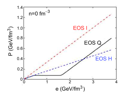
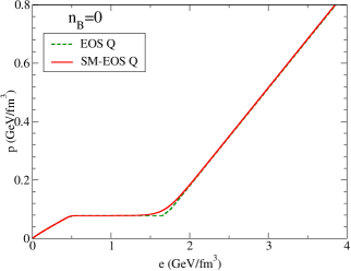
Figure 1.5: Equation of state for numerical simulations.

1.3 AdS/CFT

In quantum field theory, the partition function is written as

$$Z_{QFT} = \int D\phi e^{i\int d^{4}x(\mathcal{L}_{0}+g\mathcal{L}_{1})}$$ (1.9)

$$= \int D\phi e^{i\int d^{4}x\mathcal{L}_{0}}[1+ig\int d^{4}\mathcal{L}_{1}+O(g^{2})]\;,$$

where $D$ denotes functional integrals of the fields $\phi$, $g$ is the coupling constant, $\mathcal{L}_{0}$ and $\mathcal{L}_{1}$ are Lagrangian for the free and the first order interacting parts, respectively. For $g\ll 1$, the theory is weakly coupled, and the perturbation works well. If $g\gg 1$, higher order contributions is not negligible and all orders in the expansion should be summed. It is difficult to describe a strongly coupled system due to its non-linear and non-perturbative feature.

In recent years a new technique to deal with strongly coupled systems in gauge theory has been developed, made use of the string/gauge duality or the AdS/CFT duality proposed by Maldacena and many others [114, 115, 116]. Here AdS and CFT are abbreviations for anti-de Sitter space and conformal field theory, respectively. In the ’t Hooft limit or large $N$ limit (with $N$ the dimension of fundamental representation of $SU(N)$ group), the action of the open strings is equivalent to that of a conformal $SU(N_{c})$ theory. In the classical limit (i.e. the gravitons are almost free), the weakly coupled closed strings (free gravitons) in a curved space correspond to the strongly coupled open strings in a flat space. Finally, the strongly coupled field conformal theory in a flat space is equivalent to the theory of closed strings in curved space.

Policastro, Son and Starinets first used AdS/CFT duality to compute the transport coefficients of sQGP [21] and derived the ratio of $\eta/s\gtrsim 1/4\pi$, which is consistent to the RHIC data. After that, there are more developments in this field. Up to date three main applications of AdS/CFT duality have been explored. The first one is to use pure AdS/CFT to compute quantities of QCD-like CFT at very high temperatures (see e.g. Ref.[117, 118, 119] for the energy loss, Ref. [120, 121] for the potential of heavy quarks, Ref. [121, 122, 123, 124] for the screening length ). The second one is to use the so-called AdS/QCD to calculate the properties of hadrons (see e.g. Ref.[125] and Ref.[126, 127] for the Sakai-Sugimoto model). The third one is the correspondence between gravity and condense matter theory (CMT), which is the so-called AdS/CMT, see e.g. Ref.[128, 129, 130, 131] for strongly coupled superconductivity and superfluidity, Ref.[132, 133] for the non-Fermi liquids. More reviews on applications of AdS/CFT duality can be found in Ref. [134, 135, 136, 137] for the pure AdS/CFT, Ref.[138, 139, 140] for superconductivity and superfluidity, Ref. [141] for jets and partons, Ref. [142] for the deconfinement phase transition and Ref. [50, 143, 144] for the fluid dynamics.

In the pure AdS/CFT, two main quantities, the (retarded) Green functions and Wilson loops, can be computed via the duality.

1.3.1 Green functions

The AdS/CFT duality means that the partition function $Z_{QFT}[J]$ in the conformal theory is equivalent to the partition function $Z_{string}[\phi]$ in the classical string theory. In this case, one finds

$$Z_{QFT}[J] = e^{iS_{string}[\phi_{cl}]}\;,$$ (1.10)

where $J$ the source coupled to the operator $O$ and $S_{string}$ is the action of the classical gravity and

$$Z_{QFT}[J]=\int D\phi exp\left(iS+i\int d^{4}xJO\right)\;.$$

The Green functions in the CFT is associated to the derivatives of the action in the AdS space, e.g. the two-point Green function of $O$ is given by the functional derivatives of $S[\phi_{cl}]$ with respect to the boundary value of $\phi$,

$$G(x-y) = \left.\frac{\delta^{2}Z_{QFT}[J\phi]}{i^{2}\delta J(x)\delta J(y)}\right|_{J=0}$$ (1.11)

$$= -\left.\frac{\delta^{2}S_{string}[\phi_{cl}]}{\delta J(x)\delta J(y)}\right|_{z\rightarrow 0,\;\phi=J}\;.$$

The problem to compute Green functions in a strongly coupled quantum field theory is made to compute the classical action of gravity.

Based on the work of Ref.[21], we study sQGP with the radial expansion and Bjorken boost invariance. The information of the sQGP is encoded on the boundary of AdS space via the holographic renormalization. The evolution of the shear viscosity as a function of proper time can be obtained via the Kubo formula for the retarded Green function given by the AdS/CFT duality, see Chap. 5 for detail.

1.3.2 Wilson loops

It is well-known that the gauge invariant Wilson loops for quark and anti-quarks in QCD can be written in the form

$$W[C]=e^{-V(R)T}=e^{-\sigma A(C)}\;,$$ (1.12)

where $C$ is a contour which is usually chosen as a rectangle in Euclidean space-time with the area $A(C)=RT$, $R$ is the distance between quarks and anti-quarks, $T$ is the imaginary time, $V$ is the potential and $\sigma=V(R)/R$ is the string tension.

Figure 1.6: Wilson loops in AdS/CFT duality.

As shown in Fig.1.6, the area of the contour $C$ can be obtained by integrating over of the world-volume of the strings. These integrals are given by the Nambu-Goto action. In this case, the Wilson loops are found to be

$$W[C]=Z_{string}[C]=e^{-(S_{string}-l\phi)}\;,$$ (1.13)

where $l$ is the length of the loop $C$ and $\phi$ is the mass field. In order to renormalize the potential of heavy quarks, the contributions from the mass of strings $l\phi$ must be removed.

In the standard AdS metric, the potential for quarks and anti-quarks is given by [137],

$$V_{q\bar{q}}(R)=-\frac{4\pi^{2}}{\Gamma(1/4)^{4}}\frac{\sqrt{2g_{YM}^{2}N_{c}}}{R}\;,$$ (1.14)

where $g_{YM}$ is the coupling constant of the super Yang-Mills theory and also see Ref. [120, 121] for the higher order contributions. This potential is strongly related to the phenomena in high energy physic, e.g. the jet quenching [117, 118, 119].

In this thesis, a Wilson-loop-like model will be used to investigate the property of high spin baryons in the QGP in Chap. 5. The quarks located at the boundary of AdS space are connected to a probe D5 brane by superstrings. The configurations of strings give the screening length of baryons as a function of spin and temperature. A Regge-like behavior, i.e. the total angular momentum is proportional to the energy squared, is also found.

1.4 Fluid dynamics with triangle anomalies

The vorticity vanishes in the first order theory of fluid dynamics due to the parity conservation. However, the analysis of the power counting in Eq.(2.83) indicates that the vorticity has the same order as other dissipative terms (e.g. shear stress tensor or bulk viscous pressure) in the first order theory. It implies that some terms related to vorticity are absent in the previous treatment (2.84).

Recently, the relativistic fluid dynamics corresponding to charged black-branes through the AdS/CFT duality was found to have two new terms associated with the axial anomalies in the first order theory [145, 146] (see, e.g, Ref. [147] about the holographic model with multiple/non-Abelian symmetries, or Ref. [148] for the Sakai-Sugimoto model). The authors of Ref. [149] have derived these new terms in relativistic fluid dynamics with triangle anomalies. Also see Ref. [150] about the similar result obtained in microscopic theory of the superfluid.

Actually, the anomalous fluid dynamics is closely related to the Chiral Magnetic Effect (CME) in heavy ion collisions [151, 152, 153, 154]. The separation of the left- and right-hand particles or anti-particles leads to macroscopic currents in the case of strong electromagnetic field. This effect is called CME. In comparison with CME, the separation of left- and right-hand particles given by vorticity is also called Chiral Vorticity Effect (CVE) [154]. The separation of chirality can be realized by the change of the topological charge [151] or the quantum triangle anomalies [149, 154]. Therefore, it is necessary to introduce an additional term proportional to the magnetic field in the conserved currents $j^{\mu}\propto B^{\mu}$. And the vorticity related to the magnetic field will also be introduced to the conserved currents $j^{\mu}\propto\omega^{\mu}$, where

$$\omega^{\mu}=\epsilon^{\mu\nu\alpha\beta}u_{\nu}\partial_{\alpha}u_{\beta}\;,$$ (1.15)

is defined in Ref. [149]. Here $\epsilon^{\mu\nu\alpha\beta}=1,-1$ for that the order of Lorentz indices $\left(\mu\nu\alpha\beta\right)$is an even/odd permutation of $(0123)$.

The anomalous fluid will be studied in a kinetic approach in Chap. 6. The transport coefficients for the vorticity will also be obtained.

Chapter 2 Basics of hydrodynamics and kinetic theory

Fluid dynamics is an effective theory for any interacting theories in long wavelength limit. Recently, it is widely used to describe the data in many aspects of the high heavy ion collisions [15, 43, 44, 45].

In this chapter, we will give a brief introduction to the basics of the hydrodynamics and kinetic theory. The basic conservation equations of fluid dynamics are given in Sec. 2.1. The first order theory of the fluid, called the relativistic Navier-Stokes equations, is shown in Sec. 2.2. Then we introduce the classic and quantum Boltzmann equation in Sec. 2.3 and 2.4, respectively. In Sec. 2.5, we give a short review to the complete second order theory of the fluid dynamics via kinetic theory.

2.1 Conservation equations

The basic fluid dynamic equations are the conservation equations of energy-momentum and charge

$$\partial_{\mu}T^{\mu\nu} = 0\;,$$ (2.1)

$$\partial_{\mu}j^{\mu} = 0\;,$$ (2.2)

where $T^{\mu\nu}$ is the energy-momentum tensor and $j^{\mu}$ is the charge current. Here we consider the homogenous fluid with only one particle species.

The tensor decomposition of $T^{\mu\nu}$ with respective to the fluid velocity $u^{\mu}$ reads

$$T^{\mu\nu}=\epsilon u^{\mu}u^{\nu}-(P+\Pi)\Delta^{\mu\nu}+(h^{\mu}u^{\nu}+h^{\nu}u^{\mu})+\pi^{\mu\nu}\;,$$ (2.3)

where $\epsilon$, $h^{\mu}$, $P$ , $\Pi$ and $\pi^{\mu\nu}$ are the energy density, the heat flux current, the pressure, the bulk pressure and the shear stress tensor, respectively, and $\Delta^{\mu\nu}=g^{\mu\nu}-u^{\mu}u^{\nu}$ is the projector onto the $3$-space orthogonal to $u^{\mu}$. Here the velocity is time-like and normalized to $1$, i.e. $u^{\mu}u_{\mu}=1$. In a Lorentz boosted frame, the velocity is given by

$$u^{\mu}=\gamma(1,\,\overrightarrow{v})\;,$$ (2.4)

where $\gamma$ is the Lorentz factor $\gamma=\sqrt{1-v^{2}}$. On the other hand, these thermal quantities can also be expressed by $T^{\mu\nu}$,

$$\epsilon=u_{\mu}u_{\nu}T^{\mu\nu}\;,\quad P+\Pi=-\frac{1}{3}\Delta^{\mu\nu}T_{\mu\nu}\;,$$

$$\pi^{\mu\nu}=P^{\mu\nu\alpha\beta}T_{\alpha\beta}\;,\quad h^{\mu}=\Delta^{\mu\nu}T_{\nu\alpha}u^{\alpha}\;,$$ (2.5)

where

$$P^{\mu\nu\alpha\beta}=\frac{1}{2}\left(\Delta^{\mu\alpha}\Delta^{\nu\beta}+\Delta^{\mu\beta}\Delta^{\nu\alpha}\right)-\frac{1}{3}\Delta^{\mu\nu}\Delta^{\alpha\beta}\;,$$ (2.6)

is the symmetric rank-four projection operator. By construction, $\pi^{\mu\nu}$ is traceless $\pi_{\mu}^{\mu}=0$ and $\pi^{\mu\nu}u_{\nu}=h^{\mu}u_{\mu}=0$ since $u^{\mu}\Delta_{\mu\nu}=0$.

The tensor decomposition of the conserved current $j^{\mu}$ reads

$$j^{\mu}=nu^{\mu}+\nu^{\mu}\;,$$ (2.7)

where $n$ is the number density and $\nu^{\mu}$ is the diffusion current. By construction,

$$n=u_{\mu}j^{\mu}\;,\qquad\nu^{\mu}=\Delta^{\mu\nu}j_{\nu}\;.$$ (2.8)

Using these tensor decompositions in Eq.(2.1, 2.2), we obtain

$$\dot{n}+n\theta+\partial_{\mu}\nu^{\mu} = 0\;,$$

$$\dot{\epsilon}+(\epsilon+P+\Pi)\theta-\partial_{\mu}h^{\mu}-h^{\mu}\dot{u}_{\mu}-\pi^{\mu\nu}\partial_{\mu}u_{\nu} = 0\;,$$

$$\Delta^{\mu\alpha}\partial_{\alpha}(P+\Pi)-(\epsilon+P)\dot{u}^{\mu}-\Pi\dot{u}^{\mu}-\Delta^{\mu\alpha}\dot{h}_{\alpha}$$

$$-h^{\mu}\theta-h^{\alpha}\partial_{\alpha}u^{\mu}-\Delta^{\mu\alpha}\partial^{\beta}\pi_{\alpha\beta} = 0\;,$$ (2.9)

which represent the conservation of charges and energy, the acceleration of the fluid, respectivley. Here $\dot{A}$ denotes $\frac{d}{d\tau}A=u^{\mu}\partial_{\mu}A$. The $\theta=\partial^{\mu}u_{\mu}$ is the expansion scalar.

For the sake of simplicity, people usually consider two special frames for the fluid dynamics. The first one is the Landau frame or energy frame [155]. In this frame, the velocity of the fluid $u_{E}^{\mu}$ is defined to describe the energy flow

$$u_{E}^{\mu}=\frac{T_{\nu}^{\mu}u_{E}^{\nu}}{\sqrt{u_{E}^{\alpha}T_{\alpha}^{\beta}T_{\beta\gamma}u_{E}^{\gamma}}}=\frac{1}{\epsilon}T_{\nu}^{\mu}u_{E}^{\nu}\;,$$ (2.10)

which is related to $u^{\mu}$ and $h^{\mu}$ via

$$u_{E}^{\mu}=u^{\mu}+\frac{1}{\epsilon+P}h^{\mu}\;,$$ (2.11)

Then the heat flux current $h^{\mu}$ vanishes. The second frame is the Eckart frame [156]. In this frame, the velocity $u_{N}^{\mu}$ is used to describe the charge flow

$$u_{N}^{\mu}=\frac{j^{\mu}}{\sqrt{j^{\mu}j_{\mu}}}\;,$$ (2.12)

with

$$u_{N}^{\mu}=u^{\mu}+\frac{1}{n}\nu^{\mu}\;.$$

Then the diffusion current vanishes. Throughout the thesis, only the Landau frame will be used. For convenience, the following quantities is also used

$$q^{\mu}=h^{\mu}-\frac{n}{\epsilon+P}\nu^{\mu}\;,$$ (2.13)

which is $h^{\mu}$ in Eckart frame and $-\frac{n}{\epsilon+P}\nu^{\mu}$ in Landau frame.

For a given fluid (the velocity $u^{\mu}$ is fixed), there are 15 unknown parameters in the equations of fluid dynamics. However, the choice of the frame does not reduce the number of the parameters since in Eckart frame the $\nu^{\mu}=0$ and in Landau frame $h^{\mu}=0$, then the velocity $u^{\mu}$ is not fixed.

2.2 Navier-Stokes approximation

2.2.1 Equilibrium state

The first law of thermodynamics read

$$d\epsilon = Tds+\mu dn\;,$$

$$dP = sdT+nd\mu\;,$$ (2.14)

where $s$ is the entropy density, $T$ is the temperature and $\mu$ is the chemical potential. The entropy density is given by the Durham-Gibbs relation

$$s=\frac{\epsilon+P}{T}-\alpha n\;,$$ (2.15)

where $\alpha=\mu/T$. Rewriting Eq.(2.14) with the Durham-Gibbs relation, the following equation is obtained

$$d(P\beta) = nd\alpha-\epsilon d\beta\;.$$ (2.16)

By introducing the new variable $\beta^{\mu}$

$$\beta_{\mu}=\beta u_{\mu}\;,$$

with $\beta=T^{-1}$, the Eq. (2.16) becomes

$$d(P\beta^{\mu})=j_{0}^{\mu}d\alpha-T_{0}^{\lambda\mu}d\beta_{\lambda}\;,$$ (2.17)

where $j_{0}^{\mu}=nu^{\mu}$ and $T_{0}^{\mu\nu}=\epsilon u^{\mu}u^{\nu}-P\Delta^{\mu\nu}$ are quantities in the ideal fluid. The entropy flow is then

$$s_{0}^{\mu} = P\beta^{\mu}+T_{0}^{\lambda\mu}\beta_{\lambda}-\alpha j_{0}^{\mu}\;.$$ (2.18)

The differential of the entropy flow reads

$$ds_{0}^{\mu} = -\alpha dj_{0}^{\mu}+\beta_{\lambda}dT_{0}^{\lambda\mu}\;.$$ (2.19)

2.2.2 Off equilibrium state

It is straightforward to assume that in an off equilibrium state Eq.(2.19) becomes

$$ds^{\mu}=-\alpha dj^{\mu}+\beta_{\lambda}dT^{\lambda\mu}\;.$$ (2.20)

if the system is in a state near the equilibrium one. The entropy flow (2.18) becomes

$$s^{\mu}=P\beta^{\mu}+T^{\lambda\mu}\beta_{\lambda}-\alpha j^{\mu}-Q^{\mu}\;,$$ (2.21)

where $Q^{\mu}$ is the high order deviations $j^{\mu}-j_{0}^{\mu}$, and $T^{\mu\nu}-T_{0}^{\mu\nu}$. Under the infinitesimal changes in $\alpha$ and $\beta$,

$$\alpha\rightarrow\alpha^{\prime}=\alpha+\delta\alpha\;,\qquad\beta_{\lambda}\rightarrow\beta_{\lambda}^{\prime}=\beta_{\lambda}+\delta\beta_{\lambda}\;,$$

the change of $Q^{\mu}$ is

$$Q^{\mu}-Q^{\mu\prime}=(j^{\mu}-j_{0}^{\mu})\delta\alpha-(T^{\lambda\mu}-T_{0}^{\lambda\mu})\delta\beta_{\lambda}\;.$$ (2.22)

Recalling Eqs. (2.5, 2.8), we assume that the charge and the energy densities do not change in the off-equilibrium state,

$$u_{\mu}(j^{\mu}-j_{0}^{\mu})=u_{\mu}u_{\nu}(T^{\mu\nu}-T_{0}^{\mu\nu})=0\;,$$ (2.23)

but the entropy density flow changes in the way

$$u_{\mu}(s^{\mu}-s_{0}^{\mu})=-u_{\mu}Q^{\mu}\;,$$ (2.24)

In principle the temperature and chemical potential will be changed if taking the contributions from the second order theory into account, i.e. they are not invariant under the transformation of $u^{\mu}$. In an off-equilibrium state, the temperature and chemical potential are not global, i.e. they are the functions of the location $x$.

Taking the additional term $Q^{\mu}$ into account, Eq. (2.20) and (2.21) become

$$s^{\mu} = \frac{s}{n}j^{\mu}+\beta q^{\mu}-Q^{\mu}\;,$$ (2.25)

and

$$\partial_{\mu}s^{\mu} = -(j^{\mu}-j_{0}^{\mu})\partial_{\mu}\alpha+(T^{\mu\lambda}-T_{0}^{\lambda\mu})\partial_{\mu}\beta_{\lambda}-\partial_{\mu}Q^{\mu}\;,$$ (2.26)

where $q^{\mu}$ is given in Eq.(2.13).

2.2.3 Entropy principle

Taking Eqs. (2.5, 2.8) in Eq.(2.26) and neglecting $Q^{\mu}$, the entropy production rate reads

$$\partial_{\mu}s^{\mu} = -\nu^{\mu}\partial_{\mu}\alpha-\frac{\Pi}{T}\partial_{\mu}u^{\mu}+\pi^{\mu\nu}\frac{1}{T}\partial_{\mu}u_{\nu}\;.$$ (2.27)

The second law of thermodynamics $\partial_{\mu}s^{\mu}\geq 0$ requires $\nu^{\mu},\Pi,\pi^{\mu\nu}$ be in the form

$$\pi_{NS}^{\mu\nu} = 2\eta\partial^{<\mu}u^{\nu>}\;,$$

$$\Pi_{NS} = -\zeta\theta\;,$$

$$\nu_{NS}^{\mu} = \kappa T\Delta^{\mu\nu}\partial_{\nu}\alpha\;,$$ (2.28)

which is called the Navier-Stokes (NS) approximation. Here $\eta,\zeta,$ and $\kappa$ are shear viscosity, bulk viscosity and heat conductivity, respectively. Note that in the metric convention $g^{\mu\nu}=\textrm{diag}\{+,-,-,-\}$, $\nu^{\mu}\partial_{\mu}\alpha$ must be negative,

$$\nu^{\mu}\partial_{\mu}\alpha=-\kappa T(\nabla\alpha)^{2}\;.$$ (2.29)

2.2.4 Simple Israel-Stewart theory

In Ref. [46], the authors suggest that in phenomenology the additional term $Q^{\mu}$ should include all the irreducible quantities in the first order theory

$$TQ^{\mu}=\frac{1}{2}u^{\mu}(\beta_{0}\Pi^{2}+\beta_{1}q^{2}+\beta_{2}\pi^{2})-\alpha_{0}\Pi q^{\mu}-\alpha_{1}\pi^{\mu\lambda}q_{\lambda}\;,$$ (2.30)

where $\beta_{i}$ and $\alpha_{j}$ are constants with $j=0,1,2$ and $i=0,1$.

The entropy production rate becomes [46],

$$\partial_{\mu}s^{\mu} = \beta\Pi[-\theta-\dot{\beta}_{0}\Pi-2\beta_{0}\dot{\Pi}-\beta_{0}\Pi T\partial_{\alpha}(\beta u^{\alpha})+a_{1}T\partial_{\mu}(\alpha_{0}\beta)\nu^{\mu}+\alpha_{0}\partial_{\mu}\nu^{\mu}]$$ (2.31)

$$+\beta\pi^{\mu\nu}[\partial_{\mu}u_{\nu}-\dot{\beta}_{2}\pi_{\mu\nu}-2\beta_{2}\dot{\pi}_{\mu\nu}-\beta_{2}T\partial_{\alpha}(\beta u^{\alpha})\pi_{\mu\nu}+a_{3}T\partial_{\mu}(\alpha_{1}\beta)\nu_{\nu}$$

$$+\alpha_{1}\partial_{\mu}\nu_{\nu}]+\beta\nu^{\mu}[-T\partial_{\mu}\alpha-T\dot{\beta_{1}}\nu_{\mu}-2\beta_{1}\dot{\nu}_{\mu}-\beta_{1}T\partial_{\alpha}(\beta u^{\alpha})\nu_{\mu}$$

$$+a_{2}\Pi T\partial_{\mu}(\alpha_{0}\beta)+\alpha_{0}\partial_{\mu}\Pi+a_{4}T\pi_{\mu}^{\nu}\partial_{\nu}(\alpha_{1}\beta)+\alpha_{1}\partial_{\nu}\pi_{\mu}^{\nu}]$$

where the new coefficients $a_{i}$ ($i=1,2,3,4$) satisfy $a_{1}+a_{2}=1$ and $a_{3}+a_{4}=1$. Thus the general form for the irreducible quantities are

$$\Pi = \zeta[-\theta-2\beta_{0}\dot{\Pi}+\alpha_{0}\partial_{\mu}\nu^{\mu}+a_{1}\alpha_{0}\nu^{\mu}\dot{u}_{\mu}]\;,$$

$$\pi_{\mu\nu} = 2\eta[\partial_{<\mu}u_{\nu>}-2\beta_{2}\dot{\pi}_{<\mu\nu>}+a_{3}\alpha_{{}_{1}}\dot{u}_{<\mu}\nu_{\nu>}+\alpha_{1}\partial_{<\mu}\nu_{\nu>}]\;,$$

$$\nu_{\mu} = -\kappa\Delta_{\mu}^{\nu}[-T\partial_{\nu}\alpha-2\beta_{1}\dot{\nu}_{\nu}+a_{2}\alpha_{0}\Pi\dot{u}_{\nu}+\alpha_{0}\partial_{\nu}\Pi$$ (2.32)

$$+a_{4}\alpha_{1}\pi_{\nu}^{\alpha}\dot{u}_{\alpha}+\alpha_{1}\partial_{\alpha}\pi_{\nu}^{\alpha}]\;,$$

which are the called the simplest Israel-Stewart (IS) equations. Here the approximation $\partial_{\mu}\beta\approx\beta\dot{u}_{\mu}$ has been used, and the coefficients $\beta_{i}$ and $\alpha_{i}$ are assumed independent of space-time. The complete IS equations have been discussed in Ref. [47, 48, 49].

2.3 Relativistic Boltzmann equation

The fluid dynamics is closely related to kinetic theory which is based on the Boltzmann equation. The relativistic Boltzmann equation describes the time evolution of the single particle distribution function $f(x,p)$, which is based on the following assumptions [157]:

• Only two-particle collisions, or the so-called binary collisions are considered.

• “Sto$\beta$zahlansatz” collision number ansatz, i.e., number density of binary collisions at $x$ is proportional to $f(x,p_{1})\times f(x,p_{2})$.

• $f(x,p)$ is a smoothly varying function compared to the mean free path $l_{mfp}$.

For example, in the $\phi^{4}$ interaction the size of the collision region $l_{sc}\sim\sigma^{1/2}$, where $\sigma$ is the cross section, needs to be much smaller than the mean free path $l_{mfp}\sim 1/(n\sigma)$. In that case, the particles interact in a very small region and travel freely in a long distance. For $l_{sc}/l_{mfp}\ll 1$, the semi-classical treatment of quasi-particle collisions in Boltzmann equations will be allowed.

The relativistic Boltzmann equation can be written as

$$\frac{df}{dt}=\frac{p^{\mu}}{E_{p}}\partial_{\mu}f(x,p)=C[f]\;,$$ (2.33)

where $p^{\mu}$ and $E_{p}$ are the four-momentum and the energy of the particles respectively, and $C[f]$ is the collision term. With the particle velocity as $\mathbf{v}_{p}=\mathbf{p}/E_{p}$, the relativistic Boltzmann equation is in the same form as the non-relativistic one

$$\frac{d}{dt}f=\partial_{t}f+\mathbf{v}_{p}\cdot\nabla f=C[f]\;.$$ (2.34)

The collision term $C[f]$ describes the change of the distribution function $f$ in a given time $dt$. For example, considering a two particles scattering $12\rightarrow 3p$, the collision term is given by

$$C[f] = \frac{1}{2}\int_{123}d\Gamma_{12\rightarrow 3p}[f_{1}f_{2}(1\pm f_{3})(1\pm f_{p})-(1\pm f_{1})(1\pm f_{2})f_{3}f_{p}]\;,$$ (2.35)

where

$$d\Gamma_{12\rightarrow 3p}=\frac{1}{2E_{p}}\left|T(p,\mathbf{k})\right|^{2}\underset{i=1}{\overset{3}{\prod}}\frac{d^{3}k_{i}}{(2\pi)^{3}(2E_{i})}(2\pi)^{4}\delta(k_{1}+k_{2}-k_{3}-p)\;,$$ (2.36)

with $T(p,\mathbf{k})$ the amplitude of the scattering. More details on the collision term $C[f]$ will be given in Sec. 4.1.

In the local rest frame, the charge density and the number current are given by

$$n = \int d^{3}pf(x,p)\;,$$ (2.37)

$$\overrightarrow{\mathbf{j}\,} = \int d^{3}p\overrightarrow{\mathbf{p}}f(x,p)\;.$$ (2.38)

In a Lorentz boost frame, the above can be written in a compact form as a Lorentz vector

$$j^{\mu}=nu^{\mu}=\int_{p}p^{\mu}f(x,p)\;,$$ (2.39)

where $\int_{p}=\int\frac{d^{3}p}{(2\pi)^{3}E_{p}}\;,$ and the four-velocity vector is

$$u^{\mu}=\gamma(1,\overrightarrow{\mathbf{v}})\;,$$ (2.40)

with $\gamma=\sqrt{1-v^{2}}$ and $\overrightarrow{\mathbf{v}}$ is fluid 3-velocity.

The energy-momentum tensor can be expressed in terms of $f$,

$$T^{\mu\nu}=\int_{p}p^{\mu}p^{\nu}f(x,p)\;.$$ (2.41)

The tensor decomposition of $T^{\mu\nu}$ and $j^{\mu}$ gives

$$n = u_{\mu}j^{\mu}=\int d^{3}pf(x,p)\;,$$

$$\epsilon = T^{\mu\nu}u_{\mu}u_{\nu}=\int d^{3}pE_{p}f(x,p)\;,$$

$$P = -\frac{1}{3}\Delta^{\mu\nu}T_{\mu\nu}=-\frac{1}{3}\int_{p}\left|\overrightarrow{\mathbf{p}}\right|^{2}f(x,p)\;,$$ (2.42)

If the particles are massless, we have the equation of state for the prefect or conformal fluid is obtained

$$\epsilon=3P\;.$$ (2.43)

In relativistic fluid dynamics, the distribution function $f_{0}(x,p)$ in an equilibrium state is

$$f_{0}(x,p)=\frac{A_{0}}{e^{\beta(u\cdot p)-\alpha}-a}\;,$$ (2.44)

where $a=0,\pm 1$ are for Boltzmann, Bose and Fermi distributions, respectively and

$$A_{0}=\frac{d_{g}}{(2\pi)^{3}}\;,$$

with $d_{g}$ the particle’s degree of freedom.

2.3.1 Juttner distribution

The relativistic Boltzmann distribution is also called the Juttner distribution. For the sake of simplicity, all thermal quantities are evaluated in the local rest frame. The number density is given by

$$n=A_{0}e^{\mu/T}4\pi m^{2}TK_{2}(z)\;,$$ (2.45)

where $K_{2}$ is the Modified Bessel function of the second kind and $z=\frac{m}{T}$. The pressure is

$$P = A_{0}e^{\mu/T}4\pi m^{2}T^{2}K_{2}(z)\;.$$ (2.46)

Then the Clapeyron equation $PV=nRT$ is obtained from Eqs.(2.45, 2.46)

$$P=nT\;,$$ (2.47)

where $k_{B}=1$. The energy density is

$$\epsilon = A_{0}e^{\mu/T}4\pi[3m^{2}T^{2}K_{2}(z)+m^{3}TK_{1}(z)]$$ (2.48)

$$= 3nT+nm\frac{K_{1}(z)}{K_{2}(z)}\;,$$

which is identical to the relativistic Boltzmann-Gibbs statistics.

2.3.2 Conservation laws

The Boltzmann equation is used to describe a system in or close to an equilibrium state. There are conserved quantities because of the time reverse symmetry in the microscopic state. Assuming that the quantity $\Psi$ is conserved during the binary collision $12\rightarrow 3p$ :

$$\Psi_{1}+\Psi_{2}=\Psi_{3}+\Psi_{p}\;,$$ (2.49)

then the macroscopic conservation law will be

$$\partial_{\mu}\left[\int_{p}\Psi_{1}p^{\mu}f(x,p)\right]$$ (2.50)

$$= \int d^{3}p\Psi_{1}C[f]$$

$$= \frac{1}{2}\int_{123}d\Gamma d^{3}p\Psi_{1}[f_{1}f_{2}(1\pm f_{3})(1\pm f_{p})-(1\pm f_{1})(1\pm f_{2})f_{3}f_{p}]$$

$$= \frac{1}{4}\int_{123}d\Gamma d^{3}p[\Psi_{1}+\Psi_{2}-\Psi_{3}-\Psi_{p}][f_{1}f_{2}(1\pm f_{3})(1\pm f_{p})]$$

$$= 0\;.$$

Choosing $\Psi=1,$ and $p^{\mu}$, the conservation equations for the charge density and energy-momentum are obtained

$$\partial_{\mu}j^{\mu} = \int_{p}p^{\mu}\partial_{\mu}f(x,p)=0\;,$$

$$\partial_{\mu}T^{\mu\nu} = \int_{p}p^{\mu}p^{\nu}\partial_{\mu}f(x,p)=0\;.$$ (2.51)

The conservation laws follow Eq.(2.49). If Eq.(2.49) is not fulfilled or the time reverse symmetry is broken (i.e. the amplitude of the scattering $12\rightarrow 3p$ is not equal to that of the inverse scattering) , the charge and energy-momentum will not be conserved. For instance, considering the triangle anomalies (i.e. the right-hand quarks will become to left-handed quarks if the topological charge is $1$), the time reverse symmetry is broken; therefore the quark number is not conserved due to

$$\partial_{\mu}j^{\mu}=C\mathbf{E}\cdot\mathbf{B}\;,$$ (2.52)

where $\mathbf{E}$ and $\mathbf{B}$ are the electric and magnetic field, respectively. Here $C$ is the constant determined by the quantum field theory. More discussions on this topic will be presented in Chap. 6.

2.4 Kadanoff-Baym equation

The Boltzmann equation can be derived from the Kadanoff-Baym (KB) equation in quantum field theory via gradient expansion. In this section we will derive the Kadanoff-Baym equation from Dyson-Schwinger (DS) equation in the closed-time-path formalism. Then we will show how the Boltzmann equation can be derived from the KB equation. There are many references about the closed-time-path formalism and derivation of the Boltzmann equation from the KB equation, see e.g. Ref. [158, 159, 160, 161, 162, 163, 164, 165, 166, 167, 168, 169].

We consider a fermionic system in quantum field theory, the two-point Green function for a fermion is defined as

$$iG(x_{1},x_{2})\equiv iG(1,2)=\left\langle T_{t}[\psi_{H}(1)\overline{\psi}_{H}(2)]\right\rangle\;,$$ (2.53)

where the operator $T_{t}$ is the causal time-ordering operator and $H$ denotes the Heisenberg picture. In order to describe a non-equilibrium system, the closed time path formalism is proposed by Keldysh and Schwinger, see Fig. 2.1. Then the two-point Green function on the contour $C$ is written as

$$iG(1,2) = \left\langle T_{C}[\psi_{H}(1)\overline{\psi}_{H}(2)]\right\rangle$$ (2.54)

$$= \left\langle T_{C}\left\{\exp\left[i\int_{C}d^{4}x\mathcal{L}_{I}\right]\psi_{I}(1)\overline{\psi}_{I}(2)\right\}\right\rangle\;,$$

where $I$ denotes the interaction picture and $\mathcal{L}_{I}$ is the interacting part of the Lagrangian. The retarded and advanced Green functions are given by

$$G^{R}(1,2)\equiv G(1,2)-G^{<}(1,2)\;,\qquad G^{A}(1,2)\equiv G(1,2)-G^{>}(1,2)\;,$$ (2.55)

where Feynman propagator $G(1,2)$ is defined by

$$G(1,2)=\theta_{C}(t_{1}-t_{2})G^{>}(1,2)+\theta_{C}(t_{2}-t_{1})G^{<}(1,2)$$

with $\theta_{c}(x)$ the Heaviside step function in the closed time path $C$.

Figure 2.1: Closed time path.

The Dyson-Schwinger equation reads

$$G^{-1}(1,2)=G_{0}^{-1}(1,2)+\Sigma(1,2)\;,$$ (2.56)

where $G_{0}$ is the Green function for the free particles and $\Sigma$ is the self-energy (normally with an $i=\sqrt{-1}$ as $i\Sigma$) which can be also written as

$$\Sigma(1,2)=\Sigma^{\delta}(1,2)\delta(t_{1}-t_{2})+\theta_{C}(t_{1}-t_{2})\Sigma^{>}(1,2)+\theta_{C}(t_{2}-t_{1})\Sigma^{<}(1,2)\;.$$ (2.57)

The solution of the Dyson-Schwinger equation can be formally written as

$$G(1,2) = G_{0}(1,2)-\int_{C}d4\int_{C}d3G_{0}(1,4)\Sigma(4,3)G(3,2)\;,$$

$$G(1,2) = G_{0}(1,2)-\int_{C}d4\int_{C}d3G(1,4)\Sigma(4,3)G_{0}(3,2)\;,$$ (2.58)

Using the Dirac equation and Eq.(2.58), in the case of $t_{1}<t_{2}$, $G^{>,<}$ fulfill the following equations

$$(i\gamma_{\mu}\partial_{1}^{\mu}-m)G^{<}(1,2) = -\int_{C}d3\delta(1,3)\Sigma^{\delta}(1,3)G^{<}(1,2)$$

$$+\int_{t_{0}}^{t_{1}}d3[\Sigma^{<}(1,3)-\Sigma^{>}(1,3)]G^{<}(3,2)$$

$$+\int_{t_{0}}^{t_{2}}d3\Sigma^{<}(1,3)[G^{>}(3,2)-G^{<}(3,2)]\;,$$

$$(-i\gamma_{\mu}\partial_{2}^{\mu}-m)G^{<}(1,2) = -\int_{C}d3\delta(1,3)\Sigma^{\delta}(1,3)G^{<}(1,2)$$ (2.59)

$$+\int_{t_{0}}^{t_{1}}d3[G^{<}(1,3)-G^{>}(1,3)]\Sigma^{<}(3,2)$$

$$+\int_{t_{0}}^{t_{2}}d3G^{<}(1,3)[\Sigma^{>}(3,2)-\Sigma^{<}(3,2)]\;,$$

Note here $\Sigma^{\delta}$ is the self-energy depending on a single time corresponding to the contribution from the mean field approximation [167]. Without loss of the generality, the $\Sigma^{\delta}$ can be neglected in normal situations.

Taking traces and the Fourier transformation for Eqs.(2.59), we obtain

$$\textrm{Tr}[(i\gamma_{\mu}\partial_{1}^{\mu}-m)G^{<}(X,q)]$$

$$= \int_{0}^{\infty}dy^{\prime}dq_{1}e^{i(q-q_{1})y^{\prime}}\textrm{Tr}\{[\Sigma^{<}(X,q_{1})-\Sigma^{>}(X,q_{1})]G^{<}(X,q)\}$$

$$+\int_{-\infty}^{0}dy^{\prime}dq_{1}e^{i(q-q_{1})y^{\prime}}\textrm{Tr}\{\Sigma^{<}(X,q)[G^{>}(X,q_{2})-G^{<}(X,q_{2})]\}\;,$$

$$\textrm{Tr}[(-i\gamma_{\mu}\partial_{2}^{\mu}-m)G^{<}(X,q)]$$

$$= \int_{0}^{\infty}dy^{\prime}dq_{1}e^{i(q-q_{1})y^{\prime}}\textrm{Tr}\{[G^{<}(X,q_{1})-G^{>}(X,q_{1})]\Sigma^{<}(X,q)\}$$

$$+\int_{-\infty}^{0}dy^{\prime}dq_{1}e^{i(q-q_{1})y^{\prime}}\textrm{Tr}\{G^{<}(X,q)[\Sigma^{>}(X,q_{2})-\Sigma^{<}(X,q_{2})]\}\;,$$

where the gradient expansion variables

$$X\equiv X_{12}=\frac{x_{1}+x_{2}}{2}\;, y\equiv y_{12}=x_{1}-x_{2}\;,$$

have been used. Combining the above two equations, we derive the covariant Kadanoff and Baym equation [170]

$$i\partial_{X}^{\mu}\textrm{Tr}[\gamma_{\mu}G^{<}(X,q)]=\textrm{Tr}[G^{>}\Sigma^{<}-G^{<}\Sigma^{>}](X,q)\;.$$ (2.60)

It is known that the two-point Green function of free particles must be proportional to the distribution function $f_{0}$ of an equilibrium state at the finite temperature. Therefore, the generalization to the Green function of the interacting particles is straightforward. One needs to use the complete distribution function $f$ to replace $f_{0}$ in Eq.(2.60). On the left-hand side of KB equation, it will give such a term as $p^{\mu}\partial_{\mu}f$ while on the right-hand side, the self-energy $\Sigma^{<,>}$ are associated with the amplitude of the interaction. Finally we end up with the Boltzmann equation (2.33)

$$\frac{d}{dt}f=p^{\mu}\partial_{\mu}f=\mathcal{C}[f]\;.$$

2.5 Complete second order theory

In hydrodynamics, in a small departure from equilibrium, it is assumed that $j^{\mu}$ and $T^{\mu\nu}$ can still provide a complete description of the non-eqilibrium states. Then there are 14 independent parameters. Correspondingly, in microscopic distribution function, a departure from equilibrium state can also be characterized by 14 parameters in $y$, the exponent in the distribution function $1/(\mathrm{Exp}(y)-a)$. The comparison between the macroscopic and microscopic approach will give part of constraints on these parameters. The method is called Grad 14 moments approximation [46].

2.5.1 First order theory

In the kinetic theory, the entropy flow is defined as

$$s^{\mu} = -\int_{p}p^{\mu}\psi(f)\;,$$ (2.61)

where

$$\psi(f) = f\ln(A_{0}^{-1}f)-a^{-1}A_{0}\Delta\ln\Delta\;,$$ (2.62)

with

$$\Delta = 1+af\;,$$

$$y(f) \equiv \psi^{\prime}(f)=\ln[A_{0}^{-1}f(x,p)/\Delta(x,p)]\;.$$ (2.63)

In an equilibrium state, we have

$$y_{0}\equiv y(f_{0})=\alpha-\beta_{\mu}p^{\mu}\;.$$ (2.64)

Since there are 14 independent parameters in $j^{\mu}$ and $T^{\mu\nu}$, the derivation from equilibrium is given by $y-y_{0}$which can be decomposed into

$$y-y_{0}=\epsilon(x)-\epsilon_{\mu}(x)p^{\mu}+\epsilon_{\mu\nu}(x)p^{\mu}p^{\nu}\;,$$

o

$$y=(\epsilon+\alpha)-(\beta_{\mu}+\epsilon_{\mu})p^{\mu}+\epsilon_{\mu\nu}p^{\mu}p^{\nu}\;,$$ (2.65)

where $\epsilon,\epsilon_{\mu},\epsilon_{\mu\nu}$ are 14 small parameters in the first order (with $\epsilon_{\mu}^{\mu}=0$).

By using the $n$-th and auxiliary moments defined in Eq.(B.1), the infinitesimal changes of $j^{\mu}$, $T^{\mu\nu}$ and the $3$-rd moment $F^{\mu\nu\lambda}$ with the full distribution $f(x,p)$ under an arbitrary variation of $f(x,p)$ are

$$\delta j^{\mu} = j^{\mu}-j_{0}^{\mu}=\epsilon J^{\mu}-\epsilon_{\nu}J^{\mu\nu}+\epsilon_{\lambda\nu}J^{\mu\nu\lambda}\;,$$

$$\delta T^{\mu\nu} = T^{\mu\nu}-T_{0}^{\mu\nu}=\epsilon J^{\mu\nu}-\epsilon_{\lambda}J^{\mu\nu\lambda}+\epsilon_{\lambda\rho}J^{\mu\nu\lambda\rho}\;,$$

$$\delta F^{\mu\nu\lambda} = F^{\mu\nu\lambda}[f]-F^{\mu\nu\lambda}[f_{0}]=\epsilon J^{\mu\nu\lambda}-\epsilon_{\rho}J^{\mu\nu\lambda\rho}+\epsilon_{\rho\sigma}J^{\mu\nu\lambda\rho\sigma}\;.$$ (2.66)

It is reasonable to assume that the charge and energy density in an off equilibrium state should be the same as those in an equilibrium state,

$$n \equiv \int_{p}(u\cdot p)f=n_{0}=\int_{p}(u\cdot p)f_{0}\;,$$

$$\epsilon \equiv \int_{p}(u\cdot p)^{2}f=\epsilon_{0}=\int_{p}(u\cdot p)^{2}f_{0}\;.$$

Thus, the equation of state will be the same as before

$$P(\epsilon,n)=P_{0}(\epsilon_{0},n_{0})\;.$$

By construction, Eq.(2.23) becomes

$$u_{\mu}\delta j^{\mu}=u_{\mu}u_{\nu}\delta T^{\mu\nu}=0\;,$$ (2.67)

or

$$\epsilon = -\left(m^{2}+4\frac{J_{31}J_{30}-J_{41}J_{20}}{D_{20}}\right)\epsilon_{**}\;,$$

$$\epsilon_{*} = 4\frac{J_{31}J_{20}-J_{41}J_{10}}{D_{20}}\epsilon_{**}\;,$$ (2.68)

where Eqs.(2.66, B.11) have been used and $A_{*}$ and $A_{**}$ denote $A^{\mu}u_{\mu}$ and $A^{\mu\nu}u_{\mu}u_{\nu}$.

Using Eq.(2.66), all quantities in the first order theory can be written in the terms of $\epsilon_{\mu}$ and $\epsilon_{\mu\nu}$. The bulk pressure, shear stress tensor and heat flow are given by

$$\Pi = -\frac{1}{3}\Delta_{\mu\nu}\delta T^{\mu\nu}=\frac{4}{3}J_{42}\Omega\epsilon_{**}\;,$$

$$\pi^{\mu\nu} = \delta T^{<\mu\nu>}=2J_{42}\epsilon^{<\lambda\rho>}\;,$$

$$q^{\mu} = \Delta_{\nu}^{\rho}u_{\mu}\delta T^{\mu\nu}-\frac{\epsilon+P}{n}\Delta^{\rho\mu}\delta j_{\mu}=-2J_{21}\Lambda\epsilon_{\alpha*}\Delta^{\mu\alpha}\;,$$ (2.69)

where $q^{\mu}$ is defined in Eq.(2.13) and

$$\Lambda = \frac{D_{31}}{J_{21}^{2}}\;,$$

$$\Omega = -3\left(\frac{\partial\ln I_{31}}{\partial\ln I_{30}}\right)+5$$ (2.70)

$$= -3\frac{J_{31}(J_{21}J_{30}-J_{20}J_{31})-J_{41}(J_{21}J_{20}-J_{10}J_{31})}{J_{42}D_{20}}+5\;.$$

Equivalently, $\epsilon$, $\epsilon_{\mu}$ and $\epsilon_{\mu\nu}$ in the Eq.(2.69) can be expressed in terms of $\Pi,\;\pi^{\mu\nu}$ and $q^{\mu}$,

$$\epsilon_{\mu\nu} = \mathcal{A}_{2}\left(3u^{\mu}u^{\nu}-\Delta^{\mu\nu}\right)\Pi-\mathcal{B}_{1}u_{(\mu}q_{\nu)}+\mathcal{C}_{0}\pi_{\mu\nu}\;,$$

$$\beta_{\mu}+\epsilon_{\mu} = \beta(u_{E})_{\mu}+\mathcal{A}_{1}\Pi u_{\mu}-\mathcal{B}_{0}q_{\mu}\;,$$

$$\epsilon = \mathcal{A}_{0}\Pi\;,$$ (2.71)

where

$$\mathcal{A}_{0} = -3\mathcal{A}_{2}\left(m^{2}+4\frac{J_{31}J_{30}-J_{41}J_{20}}{D_{20}}\right)$$

$$\mathcal{A}_{1} = -12\frac{J_{31}J_{20}-J_{41}J_{10}}{D_{20}}\mathcal{A}_{2}\;,$$

$$\mathcal{A}_{2} = \frac{1}{4J_{42}\Omega}\;,\qquad\mathcal{C}_{0}=\frac{1}{2J_{42}}\;,$$

$$\mathcal{B}_{0} = \mathcal{B}_{1}\frac{J_{41}}{J_{31}}\;,\qquad\mathcal{B}_{1}=\frac{1}{\Lambda J_{21}}\;.$$ (2.72)

2.5.2 Second order theory

For the second order theory (i.e. the theory including the derivative of the quantities in the first order theory), one needs to investigate the following $3$-rd moment with the full distribution function $f(x,p)$

$$\partial_{\alpha}F^{\alpha\mu\nu}[f]=\int_{p}p^{\mu}p^{\nu}p^{\alpha}\partial_{\alpha}f=\int_{p}p^{\mu}p^{\nu}C[f]\equiv P^{\mu\nu}\;.$$ (2.73)

The contractions of the indices in $F^{\alpha\mu\nu}$ and $P^{\mu\nu}$ give

$$F_{\nu}^{\mu\nu} = \int_{p}p^{2}p^{\mu}f=m^{2}j^{\mu}\;,$$

$$P_{\mu}^{\mu} = m^{2}\partial_{\mu}j^{\mu}=0\;.$$ (2.74)

As a rank-$2$ tensor, $P^{\mu\nu}$ can be decomposed as

$$P^{\mu\nu}=Au^{\mu}u^{\nu}+B\Delta^{\mu\nu}+2Cu^{(\mu}q^{\nu)}+D\pi^{\mu\nu}\;,$$

where $A,B,C,D$ are the integrals of the collision term.

The rank-$2$ tensor $P^{\mu\nu}$ can be written in the form

$$P^{\mu\nu}=-X^{\mu\nu\alpha\beta}\epsilon_{\alpha\beta}\;,$$ (2.75)

where $X^{\mu\nu\alpha\beta}$ is a rank-$4$ tensor. Recalling the definition (2.61), the entropy principle requires

$$0\leq\partial_{\mu}s^{\mu}=-\int_{p}\psi^{\prime}p^{\mu}\partial_{\mu}f=-\int_{p}\epsilon_{\mu\nu}p^{\mu}p^{\nu}C[f]=\epsilon_{\mu\nu}X^{\mu\nu\alpha\beta}\epsilon_{\alpha\beta}\;,$$

which implies that

$$X^{\mu\nu\alpha\beta}=X^{\alpha\beta\mu\nu}\;.$$ (2.76)

By the symmetry (2.76) and $g_{\mu\nu}X^{\mu\nu\alpha\beta}=g_{\alpha\beta}X^{\mu\nu\alpha\beta}=0$, the general form of $X^{\mu\nu\alpha\beta}$ is

$$X^{\mu\nu\alpha\beta} = \frac{1}{3}A\left(-\frac{1}{3}\Delta^{\mu\nu}\Delta^{\alpha\beta}-3u^{\mu}u^{\nu}u^{\alpha}u^{\beta}+\Delta^{\mu\nu}u^{\alpha}u^{\beta}+\Delta^{\alpha\beta}u^{\mu}u^{\nu}\right)$$ (2.77)

$$+\frac{1}{5}B\Delta^{\mu<\alpha}\Delta^{\beta>\nu}-4Cu^{(\mu}\Delta^{\nu)(\alpha}u^{\beta)}\;,$$

where $A,B,C$ are the integrals of the collision term $C[f]$ in the Boltzmann equation (2.33).

On the other hand, the tensor $\partial_{\alpha}F^{\alpha\mu\nu}[f]$ can be evaluated as

$$-X^{\mu\nu\alpha\beta}\epsilon_{\alpha\beta}$$ (2.78)

$$= \int_{p}p^{\mu}p^{\nu}p^{\alpha}f_{0}\Delta_{0}\partial_{\alpha}y$$

$$= J^{\mu\nu\alpha}\partial_{\alpha}(\alpha+\epsilon)-J^{\mu\nu\alpha\beta}\partial_{\alpha}(\beta_{\beta}+\epsilon_{\beta})+J^{\mu\nu\alpha\rho\sigma}\partial_{\alpha}\epsilon_{\rho\sigma}\;.$$

Inserting Eq.(2.71) and (2.77) into Eq.(2.78) and calculating the derivatives of all quantities step by step, the differential equations for the quantities in the first order theory give the IS equations which are identical with Eqs. (2.32). The details of the calculation can be found in Ref. [46, 57].

2.5.3 Complete IS equations

In the work [46, 57], the authors neglected the terms $\sigma^{\mu\nu}\equiv P^{\mu\nu\alpha\beta}\partial_{\alpha}u_{\beta}$, $\theta$ and $\partial_{\mu}\alpha$. However, it was pointed out in Ref. [47, 48] that these terms are in the same order as others.

Generally, there are three length scales in an effective theory for long distance limit of a given theory. The first one is the microscopic length scale $\ell_{micro}$. In a weakly coupled theory with well-defined quasi-particles, this quantity is equal to the inter-particle distance. The second one is the mesoscopic length scale $\ell_{meso}$ which is identical with the mean free path $l_{mfp}$ in the dilute gas limit. The third one is the macroscopic length scale $\ell_{macro}\sim\epsilon/\left|\partial\epsilon\right|$ describing the variety of the macroscopic quantities (e.g. the energy density $\epsilon$). Thus, $\ell_{macro}^{-1}$ is proportional to the gradients of the conserved quantities. If the so-called Knudsen number $K\equiv\ell_{meso}/\ell_{macro}$ is sufficiently small, the expansion in terms of $K$ is equivalent to a gradient expansion, i.e., the expansion in terms of powers of $l_{mfp}\partial_{\mu}$.

The ratios of the quantities in the first order theory to the energy density are proportional to $K$. For example, the ratio of bulk viscous pressure to the energy density reads

$$\frac{\Pi_{NS}}{\epsilon}\sim\frac{\zeta\partial\cdot u}{\epsilon}\sim\frac{\zeta}{s}\frac{\partial}{T}\sim l_{mfp}\partial_{\mu}\equiv K\;,$$ (2.79)

where the fundamental relation of thermodynamics, $\epsilon+P=Ts+\mu n$ has been used and

$$\frac{\zeta}{s}\sim\frac{\eta}{s}\sim\frac{1}{\lambda_{th}\sigma}\frac{1}{T^{3}}\sim\frac{1}{\sigma n}\frac{1}{\lambda_{th}}\sim\frac{l_{mfp}}{\lambda_{th}}\;,$$ (2.80)

with the help of $\eta\sim(\lambda_{th}\sigma)^{-1}$, $l_{mfp}\sim(\sigma n)^{-1}$. Here $\sigma$ is the average cross section and $\lambda_{th}\sim T^{-1}$ is the thermal wavelength. Note here the result (2.79) is independent on the ratio $\zeta/s$, i.e., the expansion in terms of $K$ (or the gradient expansion ) is available in both weakly and strongly coupled theories. The ratios of the correlations from the second order theory to the energy density are also proportional to the $K$. For example, the ratio of the $\tau_{\Pi}\dot{\Pi}$ with the relaxation time $\tau_{\Pi}$ for the bulk viscous pressure to the energy density reads

$$\frac{\tau_{\Pi}\dot{\Pi}}{\epsilon}\sim\frac{\Pi}{\epsilon}\tau_{\Pi}u\cdot\partial\sim K\frac{\zeta}{T^{4}}\partial\sim K\frac{\zeta}{s}\lambda_{th}\partial\sim K^{2}\;,$$ (2.81)

where the estimation of $\tau_{\Pi}$ is employed in Ref. [46, 49]

$$\frac{\tau_{\Pi}}{\zeta}=\beta_{0}\sim\frac{1}{T^{4}}\;.$$ (2.82)

It can be proved that the terms $\sigma^{\mu\nu}$ and

$$\omega^{\mu\nu}\equiv\Delta^{\mu\alpha}\Delta^{\nu\beta}(\partial_{\alpha}u_{\beta}-\partial_{\beta}u_{\alpha})\;,$$ (2.83)

give the same contribution as $\partial\cdot u\sim\partial_{\mu}$ in the power series of $K$. Therefore, the complete IS equations should contain these terms. Taking account of these terms, the complete IS equations is obtained in Ref. [47, 48]

$$\pi^{\mu\nu} = \pi_{NS}^{\mu\nu}-\tau_{\pi}\dot{\pi}^{<\mu\nu>}+2l_{\pi q}\nabla^{<\mu}q^{\nu>}$$

$$+2\tau_{\pi q}q^{<\mu}\dot{u}^{\nu>}+2\tau_{\pi}\pi_{\lambda}^{<\mu}\omega^{\nu>\lambda}-2\eta\hat{\delta_{2}}\pi^{\mu\nu}\theta$$

$$-2\tau_{\pi}\pi_{\lambda}^{<\mu}\sigma^{\nu>\lambda}-2\lambda_{\pi q}q^{<\mu}\nabla^{\nu>}\alpha+2\lambda_{\pi\Pi}\Pi\sigma^{\mu\nu}\;,$$

$$q^{\mu} = q_{NS}^{\mu}-\tau_{q}\Delta^{\mu\nu}\dot{q}_{\nu}+l_{q\Pi}\nabla^{\mu}\Pi-l_{q\pi}\Delta^{\mu\nu}\partial^{\lambda}\pi_{\nu\lambda}$$

$$\tau_{q\Pi}\Pi\dot{u}^{\mu}-\tau_{q\pi}\pi^{\mu\nu}\dot{u}_{\nu}+\tau_{q}\omega^{\mu\nu}q_{\nu}-\frac{\kappa}{\beta}\hat{\delta}_{1}q^{\mu}\theta$$

$$-\lambda_{qq}\sigma^{\mu\nu}q_{\nu}+\lambda_{q\Pi}\Pi\nabla^{\mu}\alpha+\lambda_{q\pi}\pi^{\mu\nu}\nabla_{\nu}\alpha\;,$$

$$\Pi = \Pi_{NS}-\tau_{\Pi}\dot{\Pi}-l_{\Pi q}\partial\cdot q$$ (2.84)

$$+\tau_{\Pi q}q\cdot\dot{u}-\zeta\hat{\delta}_{0}\Pi\theta$$

$$+\lambda_{\Pi q}q\cdot\nabla\alpha+\lambda_{\Pi\pi}\pi^{\mu\nu}\sigma_{\mu\nu}\;,$$

where $\pi_{NS}^{\mu\nu},\;q_{NS}^{\mu},\;\Pi_{NS}$ are given by Eq.(2.28) and in the dilute gases limit the values of the transport coefficients in the second order theory are given in Ref. [49]. These values can also be evaluated by other theories, such as Boltzmann equation and AdS/CFT duality. The details for computing the transport coefficients in kinetic approach will be shown in Chap. 4 and by the AdS/CFT duality in Chap. 5.

Note that in dilute gases limit, the ratios of the transport coefficients in the second order theory to the quantities in the first order theory are only the function of $\alpha$ and $\beta$. For example, as shown in Eq.(2.82), $\beta_{0}$ will be determined by the macroscopic state , and therefore will be changed with the evolution of the fluid. It is a quite different treatment in the simulation for the viscous fluid dynamics, for their simplicity, the value of $\eta$ and the relaxation time $\tau_{\pi}$ are fixed, see e.g. Ref. [104, 105].

Chapter 3 Causality and stability

The first order theory does not obey the causality [59, 60, 61, 62, 63]. The causality cannot be satisfied automatically. Therefore, there has to be constraint condition for the transport coefficients, which is called asymptotic causality condition [64, 65, 66]. On the other hand, stability is intimately related to causality [64, 65, 66]. A causal theory will be stable.

In this chapter, we investigate the causality and stability of relativistic dissipative fluid dynamics in the absence of conserved charges [65]. In a linear stability analysis of the rest frame, we obtain the asymptotic causality condition and find that the equations of relativistic dissipative fluid dynamics are always stable. In a Lorentz-boosted frame, we find the equations of fluid dynamics are stable if the asymptotic causality condition is fulfilled. The group velocity may exceed the velocity of light in a certain finite range of wave numbers. However, we demonstrate that this does not violate causality, if the asymptotic causality condition is fulfilled. Finally, we compute the characteristic velocities and show that they remain below the velocity of light if we choose the parameters fulfilled the asymptotic causality condition. The similar discussion for the dissipative currents can be found in Ref. [66].

3.1 General discussion

To demonstrate the causal problem in the first order theory, for simplicity only the heat conductivity is taken into account in Eq. (B.42) for the ideal fluid. In this case, Eq.(B.41) becomes

$$0 = \partial_{\mu}j^{\mu}$$ (3.1)

$$= -J_{20}\dot{\beta}+J_{21}\beta\theta+J_{10}\dot{\alpha}+\partial_{\mu}\nu^{\mu}\;.$$

Substituting Eq.(3.1) into Eq.(B.39) yields

$$\dot{\beta} = \frac{1}{D_{20}}[(J_{31}J_{10}-J_{21}J_{20})\beta\theta-J_{20}\partial_{\mu}\nu^{\mu}]\;,$$

$$\dot{\alpha} = \frac{1}{D_{20}J_{20}}[(J_{31}J_{20}^{2}-J_{30}J_{21}J_{20})\beta\theta-J_{20}\partial_{\mu}\nu^{\mu}]\;,$$ (3.2)

where the second line in the massless limit, i.e. $J_{30}/J_{31}=J_{20}/J_{21}=3$, becomes

$$\dot{\alpha}+\frac{\kappa}{D_{20}}[\partial^{2}-(u\cdot\partial)^{2}]\alpha=0\;.$$

In the local rest frame, the above equation can be written in the form

$$\partial_{t}\alpha=-\frac{\kappa}{D_{20}}\nabla^{2}\alpha\;.$$ (3.3)

If the chemical potential $\mu$ is fixed, Eq.(3.3) is actually the heat conduction equation

$$\frac{\partial T}{\partial t}=D\frac{\partial^{2}T}{\partial x^{2}}\;,$$ (3.4)

which gives the dispersion relation

$$\omega=iDk^{2}\;.$$ (3.5)

This implies the system is acausal since that the group speed of the signal is proportional to the wave-number $k$ [64].

To avoid this problem, the simplest way is to introduce a second order time derivative $\partial_{t}^{2}T$ in Eq.(3.4). Then Eq.(3.4) becomes a standard wave equation

$$\tau_{q}\frac{\partial^{2}T}{\partial t^{2}}+\frac{\partial T}{\partial t}=D\frac{\partial^{2}T}{\partial x^{2}}\;,$$ (3.6)

where $\tau_{q}$ has the dimension of the time. However, there must be some constraint condition for $\tau_{q}$ and $D$ since if $\tau_{q}\rightarrow 0$ the system will be acausal again.

3.2 Causality in local rest frame

The approaches to formulate a second order theory of relativistic fluid dynamics is not unique, different approaches differ only by non-linear second order terms (see e.g. Ref. [46, 47, 50, 51, 52, 53, 54, 55, 64]). These differences will vanish since a linear analysis is applied here. In that case, the evolution equations of the dissipative quantities are given by

$$\tau_{\Pi}\,\frac{d}{d\tau}\Pi+\Pi = -\zeta\,\partial_{\mu}u^{\mu}\;,$$

$$\tau_{\pi}\,P^{\mu\nu\alpha\beta}\,\frac{d}{d\tau}\pi_{\alpha\beta}+\pi^{\mu\nu} = 2\eta\,P^{\mu\nu\alpha\beta}\,\partial_{\alpha}u_{\beta}\;,$$

$$\tau_{q}\Delta^{\mu\nu}\frac{d}{d\tau}\nu_{\nu}+\nu^{\mu} = \frac{n^{2}\kappa T^{2}}{(\epsilon+P)^{2}}\nabla^{\mu}\alpha\;.$$ (3.7)

The investigation of the causality and stability for a hydrostatic background in exclusively the low- and high-wave-number limit is given by Hiscock, Lindblom and Olson [60, 61]. However, they did not find a generic anomalous behavior of the group velocity. The analysis of the causality and stability for the dissipative fluid with the bulk viscous pressure only has been done in Ref. [64], where they point out the relation between causality and stability. Since the analysis in the fluid with bulk viscosity only is similar to that with shear viscosity only [64]. In this chapter, we will make a discussion on the properties of the fluid with shear stress tensor only in the absence of the conserved charges.

For convenience, the following dimensionless parameters will be used

$$a=\frac{\eta}{s}\;,\qquad b=\frac{(\epsilon+P)\tau_{\pi}}{\eta}=\frac{\tau_{\pi}T}{a}\;,$$ (3.8)

where $\epsilon+P=Ts$ has been used in the absence of conserved charges. A $D$ dimensional ($D\geq 3$) system will be considered. The symmetric rank-four projector is in the form

$$P^{\mu\nu\alpha\beta}=\frac{1}{2}\left(\Delta^{\mu\alpha}\Delta^{\nu\beta}+\Delta^{\mu\beta}\Delta^{\nu\alpha}\right)-\frac{1}{D-1}\Delta^{\mu\nu}\Delta^{\alpha\beta}\;.$$ (3.9)

A perturbation around the hydrostatic equilibrium state is introduced

$$X=X_{0}+\delta Xe^{i\omega t-ikx}\;,$$ (3.10)

where $X=\epsilon,\pi^{\mu\nu},u^{\mu}$ with $\epsilon_{0}=\textrm{const}$, $\pi_{0}^{\mu\nu}=0$ and $u^{\mu}=(1,0,0,...)$. In the linear approximation, the perturbation quantities $\delta X$ are chosen to be

$$\delta X = (\delta\varepsilon,\delta u^{1},\delta\pi^{11},\delta u^{2},\delta\pi^{12},\ldots,\delta u^{D-1},\delta\pi^{1(D-1)},\delta\pi^{22},\delta\pi^{33},\ldots,$$ (3.11)

$$\;\;\delta\pi^{(D-2)(D-2)},\delta\pi^{23},\delta\pi^{24},\ldots,\delta\pi^{2(D-1)},\delta\pi^{34},\ldots,\delta\pi^{(D-2)(D-1)})^{T}\;,$$

constrained by the normalization condition $u^{\mu}u_{\mu}=1$, the traceless condition $\pi_{\mu}^{\mu}=0$ and the orthogonality condition $u_{\mu}\pi^{\mu\nu}=0$. The linearized fluid-dynamical equations including the evolution equations (3.7) can be written as

$$A\delta X=0\;,$$ (3.12)

where the matrix $A$ is in the form

$$A=\left(\begin{array}[]{cccc}T&0&0&0\\ 0&B&0&0\\ G&0&C&0\\ 0&0&0&E\end{array}\right)\;,$$ (3.13)

with

$$T=\left(\begin{array}[]{ccc}i\omega&f_{1}&0\\ -ikc_{s}^{2}&f_{2}&-ik\\ 0&\Gamma&f\end{array}\right)\;, G=\left(\begin{array}[]{ccc}0&\Gamma_{2}&0\\ &\ldots\\ 0&\Gamma_{2}&0\end{array}\right)_{(D-3)\times 3}\;,$$ (3.20)

$$B={\rm diag}(B_{0},\ldots,B_{0})_{(D-2)\times(D-2)}\;, B_{0}=\left(\begin{array}[]{cc}f_{2}&-ik\\ \Gamma_{1}&f\end{array}\right)\;,$$ (3.23)

$$C={\rm diag}(f,\ldots,f)_{(D-3)\times(D-3)}\;,$$

$$E={\rm diag}(f,\ldots,f)_{\frac{1}{2}(D-2)(D-3)\times\frac{1}{2}(D-2)(D-3)}\;,$$ (3.24)

where $c_{s}=\sqrt{\partial P/\partial\varepsilon}$ is the speed of sound and for convenience, the following abbreviations have been used

$$f=i\omega\,\tau_{\pi}+1\;, f_{1}=-ik\,(\epsilon+P)\;,$$

$$f_{2}=i\omega\,(\epsilon+P)\;, \Gamma=-ik\,\frac{2(D-2)}{D-1}\,\eta\;,$$

$$\Gamma_{1}=-ik\,\eta\;, \Gamma_{2}=ik\,\frac{2}{D-1}\,\eta\;.$$ (3.25)

The determinant of the matrix $A$ must vanish to avoid the trivial solutions of Eq.(3.12). Solving $\det A=0$ gives

$$f = 0\;,$$ (3.26a)

$$\det B=\left(\det B_{0}\right)^{D-2} = 0\;,$$ (3.26b)

$$\det T=\det\left(\begin{array}[]{ccc}i\omega&f_{1}&0\\ -ik\,c_{s}^{2}&f_{2}&-ik\\ 0&\Gamma&f\end{array}\right) = 0\;.$$ (3.26f)

These gives the dispersion relation for $\omega(k)$.

A nonpropagating mode with the degeneracy $(D-3)[1+(D-2)/2]$ is given by the solution of Eq.(3.26a),

$$\omega=\frac{i}{\tau_{\pi}}\;.$$ (3.27)

The so-called shear modes with the degeneracy $2(D-2)$ are given by the solutions of Eq.(3.26b),

$$\omega=\frac{1}{2\tau_{\pi}}\left(i\pm\sqrt{\frac{4\,\eta\,\tau_{\pi}}{\varepsilon+P}\,k^{2}-1}\right)\;,$$ (3.28)

when $k$ is larger than the critical wave number

$$k_{c}=\sqrt{\frac{\varepsilon+P}{4\,\eta\,\tau_{\pi}}}\equiv\frac{\sqrt{b}}{2\,\tau_{\pi}}\;.$$ (3.29)

The numerical result for Eq.(3.28) is shown in Fig. 3.1.

Figure 3.1: The real parts (left panel) and the imaginary parts (right panel) of solutions for the shear modes obtained from Eq.(3.26b). The parameters are $a=\frac{1}{4\pi}\,,\;b=6\,,\;c_{s}^{2}=\frac{1}{3}$ for the 3+1-dimensional case, $D=4$.

The solutions of Eq.(3.26f) lead to another nonpropagating mode and two propagating modes or the sound modes. The analytic solutions in the limit of small wavenumber $k$ are

$$\omega=\left\{\begin{array}[]{l}{\displaystyle\frac{i}{\tau_{\pi}}\;,}\\ {\displaystyle\pm\,k\,c_{s}+i\,\frac{\Gamma_{s}}{2}\,k^{2}\;,}\end{array}\right.$$ (3.30)

while for large wavenumber, we have

$$\omega=\left\{\begin{array}[]{l}{\displaystyle\frac{i}{\tau_{\pi}}\,\left[1+\frac{\Gamma_{s}}{\tau_{\pi}c_{s}^{2}}\right]^{-1}\;,}\\[8.5359pt] {\displaystyle\pm\,k\,c_{s}\sqrt{1+\frac{\Gamma_{s}}{\tau_{\pi}c_{s}^{2}}}+\frac{i}{2\tau_{\pi}}\,\left[1+\frac{\tau_{\pi}c_{s}^{2}}{\Gamma_{s}}\right]^{-1}\;,}\end{array}\right.$$ (3.31)

where

$$\Gamma_{s}\equiv\frac{2(D-2)}{D-1}\,\frac{\eta}{\varepsilon+P}\equiv\frac{2(D-2)}{D-1}\,\frac{\tau_{\pi}}{b}\;,$$ (3.32)

is the sound attenuation length. The numerical solutions of Eq.(3.26f) are shown in Fig. 3.2. The nonpropagating as well as other propagating modes are stable around the hydrostatic equilibrium state since all imaginary parts are positive. It is identical to the conclusion of Hiscock and Lindblom [59, 60, 61] and others [64, 65, 66].

Figure 3.2: The real parts (left panel) and the imaginary parts (right panel) of the solutions for the sound modes (full lines) and the nonpropagating mode (dashed line) obtained from Eq.(3.26f). The parameters are $a=\frac{1}{4\pi}\,,\;b=6\,,\;c_{s}^{2}=\frac{1}{3}$ for the 3+1-dimensional case, $D=4$.

The causality requies that the group velocity

$$v_{g}=\frac{\partial\textrm{Re}\omega}{\partial k}\;,$$

must be less than the speed of light. For the nonpropagating modes ${\rm Re}\,\omega=0$, the causality is associated with the behavior of the imaginary part [64]. Generally speaking, a $k^{2}$ dependence of any nonpropagating mode can be considered to violate the causality. In that case, the results in Eq. (3.27,3.30,3.31) show that two nonpropagating modes are causal. For the sound modes, the group velocity is shown in Fig. 3.3. The group velocity for the shear modes (3.28) is shown in Fig. 3.4. Unfortunately, there are divergences near the critical wave number $k_{c}$. The details for these divergences will be discussed in Sec. 3.4.

Figure 3.3: The group velocity for sound modes $v_{g}$ for $a=1/(4\pi)\,,\;D=4\,,\;c_{s}^{2}=\frac{1}{3}$, and $b=6$ (full line), $b=2$ (dashed line), as well as $b=1.5$ (dotted line). If the asymptotic causality condition (3.34) is fulfilled, the group velocity will be always smaller than the speed of light. Otherwise, the causality is violated.

Figure 3.4: The group velocity of shear modes for $D=4\,,\;b=6\,,\;c_{s}^{2}=\frac{1}{3}$, and $a=1/(4\pi)$ (full line), $a=1/4$ (dashed line), as well as $a=1$ (dotted line). The group velocity is smaller than the speed of light in the large $k$ limit since the asymptotic causality condition (3.34) is fullfiled.

Taking solutions for all modes into account, it is found that the causal condition is determined by the behavior of group velocity in large $k$ limit,

$$v_{g}^{as}=v_{g,{\rm sound}}^{{\rm as}}=\lim_{k\rightarrow\infty}\frac{\partial Re\,\omega}{\partial k}=c_{s}\,\sqrt{1+\frac{\Gamma_{s}}{\tau_{\pi}c_{s}^{2}}}\;.$$ (3.33)

Consequently, the asymptotic causality condition reads

$$\frac{\Gamma_{s}}{\tau_{\pi}}\leq 1-c_{s}^{2}\;\;\Longleftrightarrow\;\;\frac{1}{b}\leq\frac{D-1}{2(D-2)}(1-c_{s}^{2})\;.$$ (3.34)

For conformal fluids, the above causality condition is always satisfied since

$$b=2(2-\ln 2)\simeq 2.614>2\;,$$ (3.35)

where $c_{s}^{2}=1/(D-1)$ and the values of $a=\eta/s\simeq 1/(4\pi)$ and $\tau_{\pi}=(2-\ln 2)/(2\pi T)$ are derived from the AdS/CFT correspondence [50, 171, 172].

The stability of a propagating mode is associated with the the behavior of imaginary part. If the imaginary part of the frequency in this mode is always positive, the damping amplitude of perturbations will decrease with the evolution and the system is therefore stable.

Note that in local rest frame the stability of relativistic dissipative fluid dynamics is not affected by the causality. The stable propagating modes with acausal parameters can be observed in Figs. 3.1, 3.2. For instance, an acausal fluid with $D=4$ and $b=1$ is demonstrated to be stable for the shear modes in Fig. 3.1 and sound modes in Fig. 3.2, respectively.

3.3 Stability in Lorentz-boost frame

In order to demonstrate the intimate relation between causality and stability, it is necessary to consider the system in a moving frame. For simplicity, the space-time dimension is restricted to be $D=4$.

3.3.1 Boost along $x$ direction

The perturbation of the fluid velocity in a frame boosted with the constant speed $V$ along the $x$ direction is given by

$$u^{\prime\;\mu}=u_{0}^{\prime\;\mu}+\delta u^{\prime\;\mu}\;e^{i\omega t-ikx}\;,$$ (3.36)

where

$$u_{0}^{\prime\;\mu}=\gamma_{V}(1,V,0,0)\;,\quad \delta u^{\prime\;\mu}=(V\gamma_{V}\delta u^{x},\gamma_{V}\delta u^{x},\delta u^{y},\delta u^{z})\;.$$ (3.37)

The linearized fluid-dynamical equations are given by $AX=0$ with

$$X=(\delta\varepsilon,\delta u^{x},\delta\pi^{xx},\delta u^{y},\delta\pi^{xy},\delta u^{z},\delta\pi^{xz},\delta\pi^{yy},\delta\pi^{yz})^{T}\;,$$ (3.38)

and

$$A=\left(\begin{array}[]{cccc}T_{1}&0&0&0\\ 0&B_{1}&0&0\\ G_{1}&0&C_{1}&0\\ 0&0&0&E_{1}\end{array}\right)\;,$$ (3.39)

where

$$T_{1} = \gamma_{V}^{2}\left(\begin{array}[]{ccc}T_{11}&T_{12}&\;\;i\gamma_{V}^{-2}V(\omega V-k)\\ T_{13}&T_{14}&\;\;i\gamma_{V}^{-2}(\omega V-k)\\ 0&\frac{4}{3}i\eta\gamma_{V}(\omega V-k)&\;\;\gamma_{V}^{-2}F\end{array}\right)\;,$$ (3.43)

$$B_{1} = {\rm diag}(B_{01},B_{01})\;,\qquad B_{01}=\left(\begin{array}[]{cc}i\gamma_{V}(\omega-kV)(\epsilon+P)&\;\;i(\omega V-k)\\ i\eta\gamma_{V}^{2}(\omega V-k)&\;\;F\end{array}\right)\;,$$ (3.46)

$$G_{1} = \left(\frac{}{}0\qquad-\frac{2}{3}i\eta\gamma_{V}(\omega V-k)\qquad 0\right)\;,$$

$$C_{1} = E_{1}=F\;,$$ (3.47)

with

$$T_{11} = i\omega(1+V^{2}c_{s}^{2})-ikV(1+c_{s}^{2})\;,$$

$$T_{12} = i[2\omega V-k(1+V^{2})](\epsilon+P)\;,$$

$$T_{13} = i\omega V(1+c_{s}^{2})-ik(V^{2}+c_{s}^{2})\;,$$

$$T_{14} = i\left[\omega(1+V^{2})-2kV\right](\epsilon+P)\;,$$

$$F = i\gamma_{V}(\omega-kV)\tau_{\pi}+1\;.$$ (3.48)

The determinant of the matrix $A$ is $\det A=\det T_{1}\times\det B_{1}\times F^{2}$. From $F=0$, two trivial propagating modes are found

$$\omega=\frac{i}{\gamma_{V}\tau_{\pi}}+kV\;,$$ (3.49)

which correspond to nonpropagating modes in the local rest frame. From $\det B_{1}=0$, four modes corresponding to the shear modes are observed

$$\omega_{\pm}=\frac{1}{2a(b-V^{2})\gamma_{V}}\left[iT-2a(1-b)kV\gamma_{V}\pm\sqrt{-T^{2}+4iakTV\gamma_{V}^{-1}+4a^{2}bk^{2}\gamma_{V}^{-2}}\right]\;.$$ (3.50)

On the other hand, the sound modes are given by the following equation

$$c_{s}^{2}(\epsilon+P)\left[1-i\gamma_{V}\tau_{\pi}(kV-\omega)\right]\left\{k^{2}\left[V^{2}+(V-1)^{2}V\gamma_{V}^{2}+1\right]\right.$$

$$+\left.2kV\omega\left[(V-1)V\gamma_{V}^{2}-1\right]+V^{2}\omega^{2}-c_{s}^{-2}(\omega-kV)^{2}\right\}$$

$$+\frac{4}{3}i\gamma_{V}\eta(k-V\omega)^{2}\left\{kV\left[c_{s}^{2}\gamma_{V}^{2}V(1-V)-1\right]+\omega\right\}=0\;.$$ (3.51)

Figure 3.5: The imaginary parts of $\omega$ for a boost in $x$ direction with velocity $V=0.9$ . In the upper panel, the parameter set $a=\frac{1}{4\pi},\,b=6,\,c_{s}^{2}=\frac{1}{3}$ fulfills the asymptotic causality condition (3.34), while in the lower panel $a=\frac{1}{4\pi},\,b=1,\,c_{s}^{2}=\frac{1}{3}$ violates this condition. The dashed lines are for the shear modes, while the solid lines are for the sound modes.

In contrast to the results in the local rest frame, the appearance of negative imaginary parts (i.e. the theory becomes unstable) could be observed in the right panel of Fig. 3.5 where the parameter set violates the asymptotic causality condition (3.34).

3.3.2 Boost along $y$ direction

The velocity in a frame boosted with the speed $V$ along $y$ direction is given by

$$u_{0}^{\prime\;\mu}=\gamma_{V}(1,0,V,0)\;,\quad\delta u^{\prime\;\mu}=(V\gamma_{V}\delta u^{y},\delta u^{x},\gamma_{V}\delta u^{y},\delta u^{z})\;.$$ (3.52)

The matrix $A$ is

$$A=\left(\begin{array}[]{cccc}T_{2}&H_{1}&H_{2}&0\\ H_{3}&B_{2}&H_{4}&H_{5}\\ G_{2}&H_{6}&C_{2}&0\\ 0&H_{7}&0&E_{2}\end{array}\right)\;,$$ (3.53)

with

$$T_{2}=\left(\begin{array}[]{ccc}i\omega\gamma_{V}^{2}(1+c_{s}^{2}V^{2})&-ik\gamma_{V}(\varepsilon+P)&0\\ -ikc_{s}^{2}&i\omega\gamma_{V}(\varepsilon+P)&-ik\\ 0&-\frac{4}{3}ik\eta&F_{1}\end{array}\right)\;,$$ (3.57)

$$H_{1}=\left(\begin{array}[]{cccc}2i\omega V(\varepsilon+P)\gamma_{V}^{2}&-ikV&0&0\\ 0&i\omega V&0&0\\ -\frac{2}{3}i\omega V\eta\gamma_{V}&0&0&0\end{array}\right)\;,$$ (3.61)

$$H_{3}=\left(\begin{array}[]{ccc}i\omega V\gamma_{V}^{2}(1+c_{s}^{2})&-ikV\gamma_{V}(\varepsilon+P)&0\\ 0&i\omega V\gamma_{V}^{2}\eta&0\\ 0&0&0\\ 0&0&0\end{array}\right)\;,$$ (3.66)

$$B_{2}=\left(\begin{array}[]{cccc}i\omega\gamma_{V}^{2}(1+V^{2})(\varepsilon+P)&-ik&0&0\\ -ik\gamma_{V}\eta&F_{1}&0&0\\ 0&0&i\omega\gamma_{V}(\varepsilon+P)&-ik\\ 0&0&-ik\eta&F_{1}\end{array}\right)\;,$$ (3.71)

$$H_{6}=\left(\begin{array}[]{cccc}\frac{4}{3}i\omega V\gamma_{V}^{3}\eta&0&0&0\end{array}\right)\;,$$ (3.73)

$$H_{7}=\left(\begin{array}[]{cccc}0&0&i\omega V\gamma_{V}^{2}\eta&0\end{array}\right)\;,$$ (3.75)

and

$$H_{2}=\left(\begin{array}[]{ccc}i\omega V^{2}&0&0\end{array}\right)^{T}\;,$$ (3.77)

$$H_{4}=\left(\begin{array}[]{cccc}i\omega V&0&0&0\end{array}\right)^{T}\;,$$ (3.79)

$$H_{5}=\left(\begin{array}[]{cccc}0&0&i\omega V&0\end{array}\right)^{T}\;,$$ (3.81)

$$G_{2}=\left(\begin{array}[]{ccc}0&\frac{2}{3}ik\gamma_{V}^{2}\eta&0\end{array}\right)\;,$$ (3.83)

$$C_{2}=E_{2}=F_{1}\;,$$ (3.84)

where $F_{1}=i\omega\gamma_{V}\tau_{\pi}+1$.

Solving the equation $\det A=0$ gives all modes. The nonpropagating mode takes the same form as in the local rest frame,

$$\omega=\frac{i}{\gamma_{V}\tau_{\pi}}\;.$$ (3.85)

The shear modes are given by the solutions

$$\omega_{\pm}=\frac{1}{2a(b-V^{2})\gamma_{V}}\left[i\,T\pm\sqrt{-T^{2}+4a^{2}bk^{2}-4a^{2}k^{2}V^{2}}\right]\;,$$ (3.86)

and the equations for the bulk modes are

$$3c_{s}^{2}(\epsilon+P)(-i+\gamma_{V}\tau_{\pi}\omega)(k^{2}+V^{2}\gamma_{V}^{2}\omega^{2})$$

$$+\gamma_{V}\omega\left\{4k^{2}\eta+\gamma_{V}\omega\left[3i(\varepsilon+P)+4V^{2}\gamma_{V}\eta\omega-3(\varepsilon+P)\gamma_{V}\tau_{\pi}\omega\right]\right\}=0\;,$$ (3.87)

respectively.

The numerical results are shown in Fig. 3.6 with the conclusion same as the case of boost along $x$ direction. It is confirmed that if the asymptotic causality condition (3.34) is fulfilled, the system will be causal and stable. However, the reverse is not true. A stable theory may also violate the asymptotic causality condition (3.34).

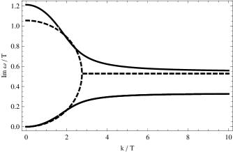
Figure 3.6: The real and imaginary parts for the shear modes (dashed lines) and sound modes (solid lines), for a Lorentz boost in $y$ direction with $a=\frac{1}{4\pi},\,b=6,\,c_{s}^{2}=\frac{1}{3},\,V=0.9\;,D=4$.

3.4 Divergences in shear modes

As mentioned in Sec. 3.2 (see also Fig. 3.4), there are divergences near the critical wave number $k_{c}$. However, the analysis for the stability of the fluid in a moving frame implies that these divergences do not affect the stability. Moreover, a lot of work [64, 65, 66] show that the causality of theory is guaranteed if the group velocity in large $k$ limit is smaller than the speed of light. This problem has also been studied in the classical electrodynamics (e.g. see [173]). The divergent group velocity may become superluminal when one analyzes the propagating modes of electromagnetic waves in some special material. However, such kind of divergences is considered to be unphysical.

The similar analysis for the divergent group velocity indicates that the divergences in shear modes do not affect the causality of the theory. The perturbation $\delta X$ in Eq.(3.10) is given by

$$\delta X(x,t)=\sum_{j}\int d\omega\,\widetilde{\delta X}_{j}(\omega)\,e^{i\omega t-ik_{j}(\omega)x}\;,$$ (3.88)

where $j$ denotes the different modes and $k_{j}(\omega)$ is the inverted $\omega(k)$ of the respective mode. The inverse Fourier transform gives the components $\widetilde{\delta X}_{j}(\omega)$

$$\sum_{j}\widetilde{\delta X}_{j}(\omega)=\frac{1}{2\pi}\int_{-\infty}^{\infty}dt\,\delta X(0,t)\,e^{-i\omega t}\;,$$ (3.89)

where $\delta X(0,t)=0$ for $t<0$ as a result of the assumption that there is no change in a fluid-dynamical variable before $t=0$. It is found that the $\sum_{j}\widetilde{\delta X}_{j}(\omega)$ is analytic in the lower half of the complex $\omega$ plane. If the asymptotic causality condition is satisfied, the imaginary part of $\omega$ is positive; therefore the singularities only arise in the upper half-plane and the system will be stable. On the other hand, if the asymptotic causality condition is violated, the singularities may appear in the lower half-plane and the system is unstable.

In order to demonstrate that the divergences of group velocity in shear modes do not violate the causality, it is necessary to compute the contour integrals (3.88) in the complex $\omega$ plane. To close the contour, the asymptotic behavior of the dispersion relations, i.e., the behavior in large $k$ limit, must be known. In large $k$ limit, the exponential in Eq.(3.88) becomes

$$\exp[i\omega t-ik_{j}(\omega)x]\rightarrow\exp\left[-i\,\frac{\omega}{v_{gj}^{{\rm as}}}\,(x-v_{gj}^{{\rm as}}\,t)\right]\;,$$ (3.90)

with

$$\lim_{k\rightarrow\infty}\textrm{Re}\omega_{j}(k)=v_{gj}^{{\rm as}}\,k\;,$$ (3.91)

where $v_{gj}^{{\rm as}}$ is given by Eq. (3.31).

If $x>v_{gj}^{{\rm as}}\,t$, the integral contour must be closed in the lower half-plane. If the asymptotic causality condition is fulfilled, Eq.(3.88) vanishes since there are no singularities in the lower half-plane. If $x\leq v_{gj}^{{\rm as}}\,t$, the integral contour must be closed in the upper half-plane. Therefore the value of $\delta X(x,t)$ in Eq.(3.88) will be nonzero because of the singularities. On the condition that the asymptotic causality condition is fulfilled , i.e., the asymptotic group velocity $v_{gj}^{as}$ is smaller than the speed of light, the locations $x$ lie within the light cone. In that case, the system is causal.

The conclusion is that the causality of theory as a whole is guaranteed by the asymptotic causality condition (3.34).

3.5 Characteristic velocity

The fluid-dynamical equations with nonlinear effect can be written as

$$\left(A_{ab}^{t}\partial_{t}+A_{ab}^{x}\partial_{x}+A_{ab}^{y}\partial_{y}\right)Y_{b}=B_{a}\;,$$ (3.92)

with $Y_{b}^{T}=(\varepsilon,u^{x},u^{y},\pi^{xx},\pi^{xy})$ and $B_{a}^{T}=(0,\;0,\;0,\;\pi^{xx},\;\pi^{xy})$. The expressions of the matrix $A$ are given in the Appendix A. The characteristic velocities are given by the solution of the following equations [59, 60, 61, 62, 63]

$$\det(v_{x}A^{t}-A^{x}) = 0\;,$$

$$\det(v_{y}A^{t}-A^{y}) = 0\;.$$ (3.93)

In the local rest frame, the characteristic velocities are given by

$$v_{x}=v_{y}=\left\{\begin{array}[]{l}0\;,\\ {\displaystyle\pm\sqrt{\frac{1}{b}}\;,}\\ {\displaystyle\pm\sqrt{\frac{1}{b}+c_{s}^{2}}\;.}\end{array}\right.\;,$$ (3.94)

The numerical results for the $b$ dependence of one of the five characteristic velocities are shown in Fig. 3.7.

The characteristic velocity which includes all the non-linear effect of the fluid dynamics also show that the system will be causal if the asymptotic causality condition is fulfilled.

Figure 3.7: One of the five characteristic velocities given by Eq.(3.93) with $u^{\mu}=(\sqrt{5}/2,\;1/2,\;0),\;\pi^{xx}=\pi^{xy}=0$, and $c_{s}^{2}=1/2$.

3.6 Discussion

In this chapter, the analysis of causality and stability of the fluid dynamical equations is performed. Considering a linear analysis, the so-called asymptotic causality condition (3.34) is obtained. The divergences in shear modes are also observed. However, the analysis from the contour integrals show that the causality as a whole is determined by the asymptotic causality condition. The stability is found to be intimately related with the causality of the system in a Lorentz boosted frame. The system will be always stable if the asymptotic causality condition (3.34) is fulfilled. More work on this topic could be found in Ref. [65] for the competition of bulk and shear viscosity, Ref. [66] for the analysis of the fluid dynamics with the heat conductivity only.

From the asymptotic causality condition, it is found that the NS equation is acausal if the relaxation time for shear viscosity goes to zero. On the other hand, it also implies that the equations of second order theory are not automatically causal by construction. It is easy to check that the results from the Grad’s 14 moments [46, 49] as well as the results from the AdS/CFT fulfill the asymptotic causality condition (3.34).

Chapter 4 Transport coefficients by Boltzmann equation

In chapter 2, we have introduced IS theory of hydrodynamics [46, 49, 57]. There are many transport coefficients in the theory. These coefficients cannot be determined in hydrodynamics but can only be determined in the underlying microscopic theory. The collision term in the Boltzmann equation has the microscopic nature since it is given by the invariant amplitudes of microscopic processes. In this chapter we will discuss about the procedure of computing these coefficients in the Boltzmann approach based on Ref. [70, 71, 73, 72].

In a leading order expansion of the coupling constant, there are an infinite number of diagrams in non-equilibrium field theory [174, 175]. However, it is proven that the summation of the leading order diagrams in a weakly coupled $\phi^{4}$ theory [174, 175, 176, 177, 178] or in hot QED [179] is equivalent to solving the linearized Boltzmann equation with temperature-dependent particle masses and scattering amplitudes. The conclusion is expected to hold in weakly coupled systems and can as well be used to compute the leading order transport coefficients in QCD-like theories [22, 70, 71, 102, 180], hadronic gases [181, 182, 183, 184, 185, 186].

4.1 Order expansion

The basic feature of relativistic Boltzmann equation (2.33) is shown in Sec. 2.3. In some case, we can add the external field $F^{\mu\nu}=\partial^{\mu}A^{\nu}-\partial^{\nu}A^{\mu}$ to the Boltzmann equation

$$\frac{df(x,p)}{dt} = \frac{p^{\mu}}{E_{p}}\left(\partial_{\mu}-qF^{\mu\nu}\frac{\partial}{\partial p^{\nu}}\right)f=\mathcal{C}[f]\;,$$ (4.1)

which can be written in a classical form. Here $q$ is the conserved charge, $qF^{\mu\nu}\frac{p^{\mu}}{E_{p}}=q(\mathbf{E}+\mathbf{v}^{\prime}\times\mathbf{B})$ is the classical Lorentz force with $\mathbf{v}^{\prime}\equiv\mathbf{p}/E_{p}$ the velocity of a particle.

The distribution function $f_{0}(x,p)$ in an equilibrium state is given in Eq.(2.44). It is straightforward to extend it to an off-equilibrium state is

$$f(x,p)=\frac{1}{e^{\beta(u\cdot p-\mu q)+\chi(x,p)}-a}\;,$$ (4.2)

where $\chi\sim\partial_{\mu}u_{\nu}\sim O(K)$ is a small quantity. The complete distribution function $f(x,p)$ can be expanded in terms of the power series of $K$ around an equilibrium state

$$f(x,p) = f_{0}(x,p)+f_{1}(x,p)+O(K^{2})\;,$$ (4.3)

where

$$f_{1}=-\chi(x,p)f_{0}(x,p)[1+af_{0}(x,p)]\;,$$ (4.4)

Substituting Eq.(4.3) into the Boltzmann equation (4.1) yields the Boltzmann equation in the $i$-th order

$$\frac{df_{i}}{dt}=C_{i}[f]\;,$$ (4.5)

where

$$C_{i}[f]=\sum_{n=1}^{i}C^{(n)}[f_{i-n}]\;,$$ (4.6)

with $C^{(n)}$ the $n$-th order derivative of the collision term $C[f]$. Note that the energy conservation in the process of two particles scattering $ab\rightarrow cd$, i.e. $E_{a}+E_{b}=E_{c}+E_{d}$ leads to the vanishing of $C[f_{0}]$,

$$C[f_{0}] = \frac{1}{2}\int_{abc}d\Gamma_{ab\rightarrow cp}[f_{0}^{a}f_{0}^{b}(1+af_{0}^{c})(1+af_{0}^{p})-(1+af_{0}^{a})(1+af_{0}^{b})f_{0}^{c}f_{0}^{p}]$$

$$= \frac{1}{2}\int_{abc}d\Gamma_{ab\rightarrow cp}(1+af_{0}^{c})(1+af_{0}^{p})(1+af_{0}^{a})(1+af_{0}^{b})$$

$$\quad\times\left[\frac{f_{0}^{a}f_{0}^{b}}{(1+af_{0}^{a})(1+af_{0}^{b})}-\frac{f^{c}f^{p}}{(1+af_{0}^{c})(1+af_{0}^{p})}\right]$$

$$= 0\;.$$

Here we have used

$$\frac{f_{0}^{a}f_{0}^{b}}{(1+af_{0}^{a})(1+af_{0}^{b})}=\frac{f_{0}^{c}f_{0}^{p}}{(1+af_{0}^{c})(1+af_{0}^{p})}\;,$$ (4.7)

The derivative of the $f_{0}(x,p)$ reads

$$\frac{df_{0}}{dt} = -f^{eq}[1+af^{eq}(x,p)]\left\{\frac{p^{\mu}}{E_{p}}\partial_{\mu}\left[\beta(u\cdot p-\mu q)\right]\right.$$ (4.8)

$$\left.\vphantom{\frac{p^{j}}{E_{P}}}+[q(\mathbf{E}+\mathbf{v}^{\prime}\times\mathbf{B})]\cdot\nabla_{p}\left[\beta(u\cdot p-\mu q)\right]\right\}\;.$$

It is convenient to evaluate the above equation in the local rest frame (i.e. $u^{0}=1$, $\mathbf{u}=0$),

$$\left.\frac{df_{0}}{dt}\right|_{\textrm{LRF}} = -f^{eq}[1+af^{eq}(x,p)]\left[E_{p}\partial_{t}\beta+p^{i}\left(\partial_{i}\beta+\beta\partial_{t}u_{i}\right)+\frac{p^{i}p^{j}}{E_{p}}\beta\partial_{\iota}u_{j}\right.$$ (4.9)

$$\left.+\frac{p^{\mu}}{E_{P}}q\partial_{\mu}\alpha+\beta[q(\mathbf{E}+\mathbf{v}^{\prime}\times\mathbf{B})]\cdot\frac{\mathbf{p}}{E_{p}}\right]\;.$$

Using the Eq.(B.47) in the local rest frame, and the following identity

$$p^{i}p^{j}\partial_{j}u_{i}=\left(p^{i}p^{j}-\frac{1}{3}\delta^{ij}\mathbf{p}^{2}\right)\sigma_{ij}+\frac{1}{3}\mathbf{p}^{2}\nabla\cdot\mathbf{u}\;,$$ (4.10)

with $\sigma_{ij}=\frac{1}{2}\left(\partial_{j}u_{i}+\partial_{i}u_{i}\right)-\frac{1}{3}\delta_{ij}\nabla\cdot\mathbf{u}$, we obtain

$$\left.\frac{df_{0}}{dt}\right|_{\textrm{LRF}} = -f_{0}[1+af_{0}(x,p)]\left[\left(\frac{n}{\epsilon+P}+\frac{q}{E_{p}}\right)\left(\mathbf{p}\cdot\nabla\alpha+\mathbf{p}\cdot\frac{\mathbf{E}}{T}\right)\right.$$ (4.11)

$$+\quad\left.\frac{\beta}{E_{p}}\left(p^{i}p^{j}-\frac{1}{3}\delta^{ij}\mathbf{p}^{2}\right)\sigma_{ij}\right]\;,$$

where the particles are assumed to be massless and therefore the bulk viscous pressure is vanished.

Because of the Boltzmann equation (4.5) the dissipative term $\chi$ in Eq.(4.2) can be written as

$$\chi = \frac{1}{T}\left[A_{1}(p)\left(p^{i}p^{j}-\frac{1}{3}\delta^{ij}\mathbf{p}^{2}\right)\sigma_{ij}\right.$$ (4.12)

$$\left.+A_{2}(p)\left(\frac{n}{\epsilon+P}+\frac{q}{E_{p}}\right)\left(\mathbf{p}\cdot\nabla\alpha+\mathbf{p}\cdot\frac{\mathbf{E}}{T}\right)\right]\;,$$

which indicates the fact that the heat conductivity is equal to the electric conductivity. By considering the contribution from the external fields, the $\nu^{\mu}$ in Eq.(2.28) now becomes

$$\nu^{\mu}=\kappa T\Delta^{\mu\nu}\left(\partial_{\nu}\alpha+\frac{E_{\nu}}{T}\right)\;.$$ (4.13)

4.2 Shear viscosity

To show the details of computing transport coefficients via the Boltzmann equation, we choose the shear viscosity as an example. For a review of the shear viscosity, see e.g. Ref. [187].

4.2.1 Non-relativistic system

Suppose the fluid is following along the $y$ direction with fluid velocity $v_{y}(x)$ which is a function of the transverse position $x$. The friction force per unit area felt in the $yz$ plane is proportional to the gradient of $v_{y}$ along $x$,

$$\frac{F}{A}=\eta\partial_{x}v_{y}\;,$$ (4.14)

where $\eta$ is the shear viscosity and its inverse is called the fluidity. In the molecular theory of dilute gases, one can estimate the value of shear viscous coefficient $\eta$ as Maxwell did. The number of particles which are moving through the unit area in $yz$ plane in unit time is

$$\Delta N=v_{x}fdv_{x}dv_{y}dv_{z}\;,$$ (4.15)

with $f$ the distribution function. The total momentum transferred in unit time gives the force

$$\frac{F}{A}=-\int_{-\infty}^{\infty}mv_{y}\Delta N\;,$$ (4.16)

which vanishes if using the equilibrium Maxwell distribution function. It implies that the shear viscous effect is a dissipative phenomenon in an off-equilibrium state. In order to evaluate this effect, an off-equilibrium distribution function $f=f_{0}+f_{1}$, where $f_{0}$ is the equilibrium one and $f_{1}$ is the fluctuation near the equilibrium state, is considered. The linearized Boltzmann equation $\partial_{t}f+\mathbf{v}\cdot\boldsymbol{\partial}f=0$ gives

$$v_{x}\partial_{x}f_{0}=-\frac{1}{\tau_{0}}f_{1}\;,$$ (4.17)

where the formula in the right hand side is given by the assumption $\partial_{t}(f-f^{0})=-(f-f^{0})/\tau_{0}$ with $\tau_{0}$ the time in which the system comes back to the equilibrium state. The solution of Eq.(4.17) is

$$f_{1}=-\tau_{0}v_{x}\partial_{x}f_{0}=-\tau_{0}v_{x}\frac{\partial f_{0}}{\partial v_{y}}\frac{dv_{y}}{dx}\;.$$ (4.18)

Substituting the above solution into the expression (4.14) yields the shear viscosity

$$\eta=-\int mv_{x}^{2}v_{y}\tau_{0}\frac{\partial f_{0}}{\partial v_{y}}dv_{x}dv_{y}dv_{z}=m\tau_{0}\int v_{x}^{2}f_{0}dv\;.$$ (4.19)

More simplification will be taken. In non-relativistic statistic physics, it is known that

$$m\int v_{x}^{2}f_{0}dv=nm\overline{v_{x}^{2}}=nk_{B}T\;,$$

where the $k_{B}$ is the Boltzmann constant and $n$ is the particle number density. Thus, the shear viscosity will be

$$\eta=\tau_{0}nk_{B}T\sim\frac{l_{mfp}}{\bar{v}}nk_{B}T\propto\sqrt{T}\;,$$ (4.20)

where $l_{mfp}$ is the mean free path which is proportion to $n^{-1}$. This result indicates that in non-relativistic case the shear viscosity is only a function of temperature $T$ and is independent on the number density $n$. By using the approximation that $\bar{v}_{x}\simeq\frac{1}{3}\bar{v}$ and $\bar{v}_{x}^{2}=\overline{v_{x}^{2}}$, the famous formula given by Maxwell is obtained

$$\eta=\frac{1}{3}npl_{mfp}\;.$$ (4.21)

Instead of the picture of quasi-particles, Frenkel and etc.[188] gave a simple picture for the motion of liquid molecules. The shear viscosity in a liquid is given by

$$\eta\simeq hne^{E/(k_{B}T)}\;,$$ (4.22)

where $h$ is the Planck constant and the collision time of the molecules was assumed to be $h/(k_{B}T)$ which is the shortest timescale in the liquid. In contrast to the results (4.21), the shear viscosity in the liquid decreases with temperature. Therefore the value of the shear viscosity must be minimum in the critical point of liquid-gas phase transition.

From Eq.(4.21) and Eq.(4.22), the ratio $\eta/n$ (or $\eta/\rho$, the kinetic viscosity with $\rho=mn$) is found to be a good quantity to describe the minimum value in the critical point. In QGP created by heavy ion collisions only net number of quarks is well-defined. The exact number of quarks and gluons is unknown. In that case, the ratio $\eta/n$ is not good enough to describe the properties of the fireball. The entropy density $s$ is well-defined and proportional to the $n$. Therefore, one can choose $\eta/s$ around the phase transition to replace $\eta/n$. The uncertainty relation gives $pl_{mfp}\simeq\hbar$, thus, $\eta/s\gtrsim\hbar/k_{B}\sim 1$ [26] which is an estimate of $1/(4\pi)$ from the AdS/CFT correspondence [21, 25].

4.2.2 Relativistic system and variational approach

In this section we will introduce the variational method in the Boltzmann approach to shear viscosity. We now turn to a relativistic system. A good example is the shear viscosity for a quark gluon system [70, 71, 72, 73].

The shear viscous term in Eq.(4.12) can be rewritten as

$$\chi=\beta B_{ij}\sigma_{ij}\;,$$ (4.23)

where the heat and electric conductivities are ignored and

$$B_{ij}=A_{1}(p)\left|\mathbf{p}\right|^{2}I_{ij}\;,$$ (4.24)

with

$$I_{ij}=\frac{1}{\left|\mathbf{p}\right|^{2}}\left(p^{i}p^{j}-\frac{1}{3}\delta^{ij}\mathbf{p}^{2}\right)\;.$$ (4.25)

Substituting Eq.(4.23) into the expression of $T^{\mu\nu}$ up to the first order of the power series of $K$ yields

$$\eta=\frac{1}{10T}\int_{p}\frac{1}{E_{p}}f_{p}\Delta_{p}\left|\mathbf{p}\right|^{2}I_{ij}B_{ij}(p)\equiv(S,B)\;,$$ (4.26)

where $S$ and $B$ are matrices with the components $S_{ij}=\left|\mathbf{p}\right|^{2}I_{ij}$.

On the other hand, the linearized Boltzmann equation (4.5) with $\chi$ in Eq.(4.23) reads

$$\left|\mathbf{p}\right|^{2}I_{ij}=\frac{E_{p}}{2}\int_{123}d\Gamma_{12,3p}\Delta_{1}\Delta_{2}f_{3}(\Delta_{P})^{-1}\left[B_{ij}(p)+B_{ij}(k_{3})-B_{ij}(k_{2})-B_{ij}(k_{1})\right]\;,$$ (4.27)

which involves collision terms. The above equation can be written in a compact form

$$S=CB\;,$$ (4.28)

where the matrix $C$ is determined by Eq.(4.27).

By using Eq.(4.28), Eq.(4.26) becomes

$$\eta = \frac{1}{20T}\int_{123p}d\Gamma_{12,3p}\Delta_{1}\Delta_{2}f_{3}f_{p}\left[B_{ij}(p)+B_{ij}(k_{3})-B_{ij}(k_{2})-B_{ij}(k_{1})\right]B_{ij}(p)$$ (4.29)

$$= \frac{1}{80T}\int_{123p}d\Gamma_{12,3p}\Delta_{1}\Delta_{2}f_{3}f_{p}\left[B_{ij}(p)+B_{ij}(k_{3})-B_{ij}(k_{2})-B_{ij}(k_{1})\right]^{2}$$

$$= (B,CB)\;,$$

which implies that the matrix $C$ is positive. Then we obtain

$$(S,B)=(B,CB)\;.$$ (4.30)

A straightforward way of computing the shear viscosity is to employ the solution to Eq. (4.28) in Eq.(4.26). However, there are two problems. The first one is from the numerical technique. The numerical errors in this kinds of integration equations will lead to some kinds of the divergent behavior [22, 23]. The second problem is the solutions of Eq.(4.28) might not fulfill the Eq.(4.30) since the solutions of integration equations are not unique.

Instead of solving Eq.(4.30) directly, the variational method is normally used. Eq.(4.29) can be rewritten as

$$\eta = 2(S,B)-(B,CB)$$ (4.31)

$$= (S,C^{-1}S)-(A,CA)\;,$$

where $A=B-C^{-1}S$. If Eq.(4.27) is not fulfilled, $\eta\leq(S,C^{-1}S)$ because of positive $C$. In numerical calculations, one needs to obtain the maximum value of Eq.(4.31) [22, 23].

In variational approach, we solve Eq. (4.30) instead of Eq. (4.28). The critical step is to find a good form of $A_{1}(p)$ to make $\eta$ as large as possible (see e.g. [70, 71, 72, 73, 182]). As an assumption, one could expand $A_{1}(p)$ by a set of orthogonal polynomials

$$A_{1}(p)=\left|\mathbf{p}\right|^{y}\sum_{r=0}^{r_{max}}b_{r}B^{(r)}(\beta p)\;.$$ (4.32)

where $B^{(r)}(\beta p)$ is a polynomial up to $(\beta p)^{r}$ and $b_{r}$ is its coefficient. Here $y$ is a constant to make the numerical error get the fastest convergence [72, 182]. In the numerical calculations, $y$ is chosen to be $1$ or $2$. The orthogonal condition is set to be

$$\frac{1}{15T}\int_{p}\frac{\left|\mathbf{p}\right|^{2+y}}{E_{p}}f_{p}\Delta_{p}B^{(r)}(\beta p)B^{(s)}(\beta p)=\mathcal{B}^{(r)}\delta_{r,s}\;,$$ (4.33)

where $\mathcal{B}^{(r)}$ is constant depending on the integrals in Eq. (4.33). Without loss of generality, we can assume $B^{(0)}=1$. Substituting Eq.(4.32) into Eq.(4.29) yields

$$\eta_{test} = \sum_{r,s}b_{r}b_{s}\widetilde{C}_{rs}\equiv<b|\widetilde{C}|b>\;,$$ (4.34)

where $|b>=(b_{0},b_{1},...,b_{r_{max}})^{T}$, the inner product is defined as $<A|B>=AB$ and

$$\widetilde{C}_{rs} = \frac{1}{80T}\int_{123p}d\Gamma_{12,3p}\Delta_{1}\Delta_{2}f_{3}f_{p}$$

$$\times \sum_{m,n=1}^{4}(-1)^{m+n}I_{ij}(\mathbf{p}_{m}\cdot\mathbf{p}_{n})\left(\left|\mathbf{p}_{n}\right|\left|\mathbf{p}_{m}\right|\right)^{y}B^{(r)}(\beta p_{m})B^{(s)}(\beta p_{m})\;,$$

where $p_{i}=(p,k_{1},k_{2},k_{3})$ and $\widetilde{C}$ is found to be a positive constant matrix into Eq.(4.26). Inserting Eq.(4.32), we have

$$\eta_{test} = \sum_{r}b_{r}S_{r}=<S|b>\;,$$ (4.35)

where $|S>=(S_{0},S_{1},...,S_{r_{max}})^{T}$ with the $r$-th component

$$S_{r}=\frac{1}{15T}\int_{p}\frac{1}{E_{p}}f_{p}\Delta_{p}\left|\mathbf{p}\right|^{2+y}B^{(r)}(\beta p)\;.$$ (4.36)

From Eq.(4.34) and (4.35), $|b>=\widetilde{C}^{-1}|S>$, we obtain

$$\eta_{test} = <S|\widetilde{C}^{-1}|S>$$

$$= \sum_{r,s}\int_{p}\left(\frac{1}{15T}\frac{1}{E_{p}}f_{p}\Delta_{p}\right)^{2}\left|\mathbf{p}\right|^{4+2y}B^{(r)}(\beta p)B^{(s)}(\beta p)\widetilde{C}_{rs}^{-1}(p)\;.$$

According to the orthogonality condition (4.33), only $B^{(0)}$ will survive in Eq.(4.35), then we finally obtain

$$\eta_{test}=\int\frac{1}{15T}\frac{1}{E_{p}}f_{p}\Delta_{p}\left|\mathbf{p}\right|^{2+y}b_{0}=b_{0}\mathcal{B}^{(0)}=(S_{0})^{2}(\widetilde{C}^{-1})_{00}\;.$$ (4.37)

Moreover, it is proved by the authors of Ref. [72, 73] that the value of $\eta_{test}$ will increase with $r_{max}$ increasing. Therefore, the value of $r_{max}$ depends on the numerical precision.

4.3 An example: shear viscosity of a gluon plasma

Recently perturbative QCD calculation of $\eta/s$ of a gluon plasma has raised wide attention. Xu and Greiner (XG) used a parton cascade model to calculate $\eta/s$ [69, 189]. They claimed that the dominant contribution comes from the inelastic $gg\leftrightarrow ggg$ (23) process instead of the elastic $gg\rightarrow gg$ (22) process: the 23 process is 7 times more important than 22. This result is in sharp contrast to AMY’s result [22, 23] where the 23 process only gives $\sim 10\%$ correction to the 22 process.

Both XG and AMY use kinetic theory for their calculations. The main differences are [70, 71] (i) XG uses a parton cascade model [190] to solve the Boltzmann equation and, for technical reasons, gluons are treated as a classical gas instead of a bosonic gas. On the other hand, AMY solves the Boltzmann equation for a bosonic gas. (ii) AMY approximates the $Ng\leftrightarrow(N+1)g$ processes, $N=2,3,4\ldots$, by the $g\leftrightarrow gg$ splitting in the collinear limit where the two gluon splitting angle is higher order. XG uses the soft gluon bremsstrahlung limit where one of the gluon momenta in the final state of $gg\rightarrow ggg$ is soft but it can have a large splitting angle with its mother gluon.

In an earlier attempt to resolve the discrepancy between XG’s and AMY’s results [70], a Boltzmann equation computation of $\eta$ is carried out without taking the classical gluon approximation (like AMY’s approach) but the soft gluon bremsstrahlung limit is applied to the 23 matrix element. It was found that the classical gas approximation does not cause a significant error in $\eta/s$. However, the result is sensitive to whether the soft gluon bremsstrahlung limit is imposed on the phase space or not. If this limit is imposed, the result is closer to AMY’s; if not, the result is closer to XG’s. This raises the concern whether this approximation is good for computing $\eta$.

This issue has been settled in Ref. [71] by using the exact amplitude for the 23 process, which removes both the soft gluon bremsstrahlung approximation and the collinear approximation to the 23process. The result of Ref. [71] shows that the contribution from the 23 process lies between AMY’s and XG’s result but more close to AMY’s. So the 23 process is less important than the 22 one in most range of coupling constant. This is consistent to the perturbative approach where higher order processes are only perturbation to lower order processes.

Chapter 5 Applications of AdS/CFT duality

Inspired by the great success of computing the ratio $\eta/s$ of a strongly coupled super Yang-Mills plasma by AdS/CFT duality, many work [171, 191, 192, 193, 194, 195] appear on the market about applying AdS/CFT correspondence to relativistic hydrodynamics with Bjorken boost invariance [196]. People try to establish a well-defined gravity dual to relativistic fluid dynamical by AdS/CFT duality.

In Sec. 5.1, we investigate the shear viscosity $\eta$ of strongly coupled super Yang-Mills (SYM) plasma in late time of hydrodynamic evolution with Bjorken scaling via AdS/CFT duality. We obtain the metric $g_{\mu\nu}$ in a proper time dependent $AdS_{5}$ space via holographic renormalization, whose boundary condition is given by energy-momentum tensor of the QGP with transverse expansion or radial flow. With this metric we compute $\eta$ of fluids in 0+1 and 1+1 dimension without and with radial flow. We find the ratio $\eta/s=1/(4\pi)$ in 0+1 dimension consistent with the KSS bound if next-to-leading terms in proper time are included in the equation of motion for metric perturbations. For 1+1 dimension the result is unchanged in the leading order of transverse rapidity [172].

In Sec. 5.2, we consider a string-junction holographic model of a probe baryon in the finite-temperature AdS background. We investigate the screening length for a high spin baryon. By defining the screening length as the critical separation of quarks, we compute the $\omega$ (spin) dependence of the baryon screening length numerically and find that baryons with high spin dissociate more easily. Finally, we discuss the Regge-like relation between the angular momentum $J$ and the total energy $E^{2}$ for baryons [124].

5.1 Shear viscosity in late time

5.1.1 Kubo relation

The Kubo relation can be obtained by the statistical analysis [67, 68]. Here a simple way given to derive the Kubo formula given based on Ref. [50] which is associated with the AdS/CFT duality.

The action with a source $J_{a}(x)$ and its operator $O_{a}(x)$ is written as

$$S=S_{0}+\int_{x}J_{a}(x)O_{a}(x)\;.$$

The perturbation of $J_{a}(x)$ gives

$$\left\langle O_{a}(x)\right\rangle=-\int_{y}G_{ab}^{R}(x-y)J_{b}(x)\;,$$ (5.1)

with the help of the linear response theory. Here $G_{ab}^{R}$ is the retarded Green’s function defined by

$$iG_{ab}^{R}(x-y)=\theta(x^{0}-y^{0})\left\langle[O_{a}(x),O_{b}(y)]\right\rangle\;.$$ (5.2)

It is known that the metric $g^{\mu\nu}$ as a source is coupled to $T^{\mu\nu}$ as an operator in the general theory of relativity. For the sake of simplicity, the metric $g^{\mu\nu}$ is considered as a homogeneous one $\delta_{ij}$ with a perturbation $h_{ij}(t)\ll 1$. Moreover, $h_{ij}$ is assumed to be traceless $h_{ii}=0$. In the local rest frame, i.e. $u^{\mu}=(1,0,0,0)$, the shear viscous tensor defined in Eq.(2.28) with covariant derivatives reads

$$\sigma_{xy}=2\eta\Gamma_{xy}^{0}=\eta\partial_{0}h_{xy}\;.$$ (5.3)

Considering a perturbation in the form of the plane wave $h_{ij}=(h_{0})_{ij}e^{i\omega t}$ with constant $h_{0}$ yields

$$\left\langle\sigma_{xy}\right\rangle=i\omega\eta+O(\omega^{2})\;.$$ (5.4)

Using Eq.(5.1), one obtains

$$\left\langle\sigma_{xy}\right\rangle=-\int G_{xy,ij}^{R}h_{ij}=-\int G_{xy,xy}^{R}h_{xy}\;.$$ (5.5)

Substituting Eq.(5.5) into Eq.(5.3) and taking the low frequency limit, i.e. the fluid dynamical limit,

$$\eta=\underset{\omega\rightarrow 0}{\lim}\frac{1}{\omega}\int dtdxe^{i\omega t}\theta(t)<[T_{xy}(x),T_{xy}(0)]>\;.$$ (5.6)

Then we derive the Kubo formula

$$\eta=-\underset{\omega\rightarrow 0}{\lim}\frac{1}{\omega}\mathsf{\mathrm{Im}}G_{xy,xy}^{R}(\omega,0)\;,$$ (5.7)

where in the low wave-number limit the Fourier transform of the retarded Green function gives

$$G_{xy,xy}^{R}(\omega,0)=-i\underset{k\rightarrow 0}{\lim}\int dtdxe^{-ik_{\mu}x^{\mu}}\theta(t)<[T_{xy}(t,x),T_{xy}(0,0)]>\;.$$ (5.8)

5.1.2 Hydrodynamics with Bjorken boost invariance

In heavy ion collisions, it is assumed that all particles are created in the same proper time after the collisions. In the laboratory frame, one will observe in the center region of the collisions that the particles moving fast are produced much earlier than those moving slowly due to the Lorentz transformation. So one can assume that the space rapidity $\eta=\frac{1}{2}\ln\left(\frac{t+z}{t-z}\right)$ is equal to the momentum rapidity $y=\frac{1}{2}\ln\left(\frac{p_{0}+p_{z}}{p_{0}-p_{z}}\right)$, for collisions along the $z$-direction. After some simplification, the following formula is obtained

$$\tanh y\equiv\frac{p_{z}}{p_{0}}=v_{z}=\frac{z}{t}\;,$$ (5.9)

where $\tau=\sqrt{t^{2}-z^{2}}$ is the transverse proper time.

Bjorken [196] suggested that all the thermal quantities should be independent of the rapidity $y$. It is convenient to use the coordinates $(\tau,y)$ instead of $(t,z)$. Using the coordinates $(\tau,y)$ and the equation of state $\epsilon=3P$, the thermal quantities of the ideal fluid can be solved as

$$x=x_{0}\left(\frac{\tau_{0}}{\tau}\right)^{m}\;,$$ (5.10)

where $x_{0}$ is the initial value for $x$ in the proper time $\tau_{0}$, and for $x=\epsilon,P$, $m=4/3$, for $x=T$, $m=1/3$, and for $x=s,n$, $m=1$.

In order to describe the evolution of the fluid with transverse expansion, besides $(\tau,y)$ the cylindrical coordinates will also be used

$$x^{\mu} = (\tau,y,r,\theta)\;,$$ (5.11)

with $r$ and $\theta$ are radius and azimuthal angle in transverse plane. The velocity of the fluid cells can be parametrized as

$$u^{\mu} = \frac{dX^{\mu}}{d\tau_{f}}=\frac{1}{\sqrt{1-R^{2}(\tau,r)/\tau^{2}}}\left[1,0,\frac{R(\tau,r)}{\tau},0\right]$$ (5.12)

$$\equiv \left[\cosh\alpha(\tau,r),0,\sinh\alpha(\tau,r),0\right]\;,$$

where the total proper time $\tau_{f}$ is given by $\tau_{f}=\sqrt{\tau^{2}-r^{2}}$ and $R(\tau,r)$ is an unknown function which has to be determined by the evolution equations of the fluid. For simplicity, the total baryon number density is assumed to vanish. The energy-momentum tensor reads

$$T_{\mu\nu} = \left(\begin{array}[]{cccc}-\frac{\epsilon}{3}+\frac{4}{3}\epsilon\cosh^{2}\alpha&0&-\frac{4}{3}\epsilon\sinh\alpha\cosh\alpha&0\\ 0&\frac{\rho}{3}\tau^{2}&0&0\\ -\frac{4}{3}\epsilon\sinh\alpha\cosh\alpha&0&\frac{\epsilon}{3}+\frac{4}{3}\epsilon\sinh^{2}\alpha&0\\ 0&0&0&\frac{\epsilon}{3}r^{2}\end{array}\right)\;.$$ (5.17)

The conservation equations are

$$\nabla_{\mu}T^{\mu\nu}\equiv\partial_{\mu}T^{\mu\nu}+\Gamma_{\mu\sigma}^{\mu}T^{\sigma\nu}+\Gamma_{\mu\sigma}^{\nu}T^{\mu\sigma}=0\;,$$ (5.18)

where $\Gamma_{\mu\sigma}^{\mu}$ are Christoffel symbols for the metric $\widetilde{g}_{\mu\nu}^{(0)}=\mathrm{diag}(-1,\tau^{2},1,r^{2})$. Solving Eqs. (5.18) leads to

$$\partial_{\tau}\ln\epsilon = -\frac{2}{\tau}\frac{2\cosh^{2}\alpha}{2\cosh^{2}\alpha+1}\left(1+\frac{R}{\tau}+\partial_{\tau}R\right)\;,$$

$$\partial_{\tau}\ln R = \frac{1}{\tau}\frac{R/\tau+2+2(1-\partial_{r}R)\cosh^{2}\alpha}{2\cosh^{2}\alpha+1}\;.$$ (5.19)

With a given initial condition $R(\tau_{0},r)=\xi\tau_{0}r$, where $\xi$ is set to 0.05 $\mathrm{fm}^{-1}$ given by Ref. [15, 197], the numerical results of the Eqs. (5.19) are shown in Fig. 5.1 and are identical to the results in Ref. [15, 197]. The results indicate that in this case the radial velocity is proportional to the distance, i.e. $u_{r}\sim\xi r$, and is observed to rise sharply at the early time and fall with increasing transverse proper time. The evolution of the energy density shown in Fig. 5.2 is found to damp in the power series of $\tau^{4/3}$ if the transverse expansion is negligible.

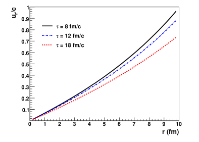
Figure 5.1: The radial velocity $u_{r}=\sinh\alpha$ as functions of $r$ and $\tau$.

Figure 5.2: The energy density as a function of $r$ and $\tau$.

5.1.3 Holographic renormalization

Generally, the AdS metric can be written in the form of Fefferman coordinates [198]

$$ds^{2} = g_{MN}dX^{M}dX^{N}=\frac{1}{z^{2}}\left[\widetilde{g}_{\mu\nu}(x,z)dx^{\mu}dx^{\nu}+dz^{2}\right]\;,$$ (5.20)

where $X^{M}=(x^{\mu},z)$ and $\widetilde{g}_{\mu\nu}(x,z)$ is the metric tensor in the 4-dimensional space. In Eq.(5.20), there is divergences at the boundary $z\rightarrow 0$. To cancel this divergence, i.e. to renormalize the metric $\widetilde{g}_{\mu\nu}$ at the boundary $z\rightarrow 0$, it is straightforward to assume that $\widetilde{g}_{\mu\nu}\sim z^{2}f(x,z)$ where $f(x,z)$ is a function free of singularities near the boundary. The authors of [199, 200] obtain the form of $f(x,z)$

$$\widetilde{g}_{\mu\nu}(x,z)=\sum_{n=0}z^{2n}\widetilde{g}_{\mu\nu}^{(2n)}(x)\;,$$ (5.21)

and prove that $\widetilde{g}_{\mu\nu}$ is the metric for a conformal theory. In the expansion (5.21), $\widetilde{g}_{\mu\nu}^{(0)}(x)$ is just the metric in the 4-dimensional flat space. The term $\widetilde{g}_{\mu\nu}^{(2)}(x)$ can be proved to vanish in a conformal theory. The term $\widetilde{g}_{\mu\nu}^{(4)}(x)$ is associated with the energy-momentum tensor of the conformal theory,

$$\widetilde{g}_{\mu\nu}^{(4)}(x)\propto\left\langle T_{\mu\nu}\right\rangle\;,$$ (5.22)

where the factor $\frac{N_{c}^{2}}{2\pi^{2}}=1$ with $N_{c}$ the number of colors. Higher order terms are given by the Einstein equation

$$R_{MN}-\frac{1}{2}g_{MN}R+6g_{MN}=0\;,$$ (5.23)

with the given initial condition $\widetilde{g}_{\mu\nu}^{(0)}(x)$ and $\widetilde{g}_{\mu\nu}^{(4)}(x)$, the cosmology constant $\Lambda=-\frac{d(d-2)}{2}=-6$. Here $R_{MN}$ and $R$ are the curvature tensor and scalar of AdS space, respectively. In this case, one finds that a conformal system is located at the boundary of an AdS space.

5.1.4 AdS metric with radial flow

The authors of Ref. [191, 192, 193, 194] suggest that one can use the holographic renormalization to regard the energy-momentum tensor of a boost invariant fireball as a boundary condition for $\widetilde{g}_{\mu\nu}$ in Eq.(5.21). By solving the Einstein equation (5.23), an AdS metric with the properties of the boost invariant fireball can be obtained.

In cylindrical coordinates, $\widetilde{g}_{\mu\nu}(x,z)$ can be cast in the form

$$\widetilde{g}_{\mu\nu}(x,z)dx^{\mu}dx^{\nu}=-Ad\tau^{2}+B\tau^{2}dy^{2}+C\left(dr^{2}+r^{2}d\theta^{2}\right)+2Dd\tau dr\;,$$

where $d\tau dr$ is off-diagonal element. It is too complicated to solve the AdS metric directly in the above form. A simplification is necessary. As argued in the last subsection, the radial velocity is negligible compared to the transverse one. Therefore, one can assume $\alpha$ in Eq.(5.17) is small, so $T^{\mu\nu}$ can be expanded in $\alpha$,

$$T_{\mu\nu} = \left(\begin{array}[]{cccc}\rho&0&0&0\\ 0&\tau^{2}\frac{1}{3}\rho&0&0\\ 0&0&\frac{1}{3}\rho&0\\ 0&0&0&r^{2}\frac{1}{3}\rho\end{array}\right)+\alpha\left(\begin{array}[]{cccc}0&0&-\frac{4}{3}\rho&0\\ 0&0&0&0\\ -\frac{4}{3}\rho&0&0&0\\ 0&0&0&0\end{array}\right)$$ (5.37)

$$+\alpha^{2}\left(\begin{array}[]{cccc}\frac{4}{3}\rho&0&0&0\\ 0&0&0&0\\ 0&0&\frac{4}{3}\rho&0\\ 0&0&0&0\end{array}\right)+O\left(\alpha^{3}\right)\;.$$

The off-diagonal terms proportional to $\alpha$ only arise in the next-to-leading order of the expansion. Therefore, the modification from the radial flow should be also in the order of $O(\alpha)$. Solving the Einstein equation (5.23) with the boundary condition given by Eq.(5.22) and (5.37) yields

$$g_{MN}=\frac{1}{z^{2}}\left(\begin{array}[]{ccccc}-\frac{(1-a)^{2}}{1+a}&0&\frac{4}{3}\alpha\frac{(1-a)^{2}}{1+a}&0&0\\ 0&\tau^{2}(1+a)&0&0&0\\ \frac{4}{3}\alpha\frac{(1-a)^{2}}{1+a}&0&1+a&0&0\\ 0&0&0&r^{2}(1+a)&0\\ 0&0&0&0&1\end{array}\right)\;.$$ (5.38)

with $a=\frac{\epsilon_{0}z^{4}}{3\tau^{4/3}}$ and $\epsilon_{0}$ is the same as the one in Eq.(5.10). Note here $a$ is set to a scaling and higher order contribution $\tau^{-1}$ is neglected in the late time $\tau\rightarrow\infty$ limit.

For $\alpha=0$, the metric is

$$ds^{2}=-\frac{(1-z^{4}/z_{H}^{4})^{2}}{1+z^{4}/z_{H}^{4}}\frac{d\tau^{2}}{z^{2}}+\frac{1+z^{4}/z_{H}^{4}}{z^{2}}[\tau^{2}dy^{2}+dr^{2}+r^{2}d\theta^{2}]+\frac{dz^{2}}{z^{2}}\;,$$ (5.39)

with the horizon of the black hole

$$z_{H}=\left(\frac{\epsilon_{0}}{3}\right)^{-1/4}\tau^{1/3}\;.$$ (5.40)

The standard D$3$ black AdS metric can be obtained from Eq.(5.39)

$$ds^{2}=-\frac{1-\widetilde{z}^{4}/\widetilde{z}_{H}^{4}}{\widetilde{z}^{2}}d\tau^{2}+\frac{d\mathbf{x}^{2}}{\widetilde{z}^{2}}+\frac{1}{1-\widetilde{z}^{4}/\widetilde{z}_{H}^{4}}\frac{d\widetilde{z}^{2}}{\widetilde{z}^{2}}\;,$$ (5.41)

with the replacement

$$z\rightarrow\widetilde{z}=\frac{z}{\sqrt{1+\frac{z^{4}}{z_{H}^{4}}}},\qquad z_{H}\rightarrow\widetilde{z}_{H}=\frac{z_{H}}{\sqrt{2}}\;.$$

The Hawking temperature can also be obtained

$$T_{H}=\frac{1}{\pi\widetilde{z}_{H}}=\frac{\sqrt{2}}{\pi z_{H}}\;.$$ (5.42)

5.1.5 Evolution of $\eta/s$

To compute the retarded Green function, the action of gravity is necessary. Generally, the action in the AdS space reads

$$I_{5D}=\frac{N^{2}}{8\pi^{2}R^{3}}\int d^{5}x(\mathcal{R}_{5D}-2\Lambda)\;,$$ (5.43)

where the contributions from the matter term $g_{\mu\nu}T^{\mu\nu}$ in AdS space is ignored. Considering a perturbation $g_{\mu\nu}=g_{\mu\nu}^{(0)}+h_{\mu\nu}$ with $h_{z\mu}=h_{\mu z}=0$ yields

$$I_{5D} = \frac{N^{2}}{8\pi^{2}}\int d^{5}x\sqrt{-g}(\mathcal{R}_{\mu\nu}-\frac{1}{2}g_{\mu\nu}\mathcal{R}+\Lambda g_{\mu\nu})h^{\mu\nu}$$ (5.44)

$$= \frac{N^{2}}{8\pi^{2}}\int d^{5}x\sqrt{-g}(\mathcal{R}_{\mu\nu}^{(0)}-\frac{1}{2}g_{\mu\nu}^{(0)}\mathcal{R}_{(0)}+\Lambda g_{\mu\nu}^{(0)})h^{\mu\nu}$$

$$+\frac{N^{2}}{8\pi^{2}}\int d^{5}x\sqrt{-g}(\delta\mathcal{R}_{\mu\nu}-\frac{1}{2}h_{\mu\nu}\mathcal{R}_{(0)}-\frac{1}{2}g_{\mu\nu}^{(0)}\delta\mathcal{R}+\Lambda h_{\mu\nu})h^{\mu\nu}$$

$$= \frac{N^{2}}{8\pi^{2}}\int d^{5}x\sqrt{-g}(\delta\mathcal{R}_{\mu\nu}-\frac{1}{2}g_{\mu\nu}^{(0)}\delta\mathcal{R}+4h_{\mu\nu})h^{\mu\nu}\;,$$

where $\mathcal{R}_{0}=-20$ and $\Lambda=-6$ have been used. For most AdS metric, the $h_{2}^{1}\equiv\phi$ is decoupled with others

$$I_{5D} \approx \frac{N^{2}}{8\pi^{2}}\int d^{5}x\sqrt{-g}(\delta R_{12}+4h_{12})h^{12}$$ (5.45)

$$= \frac{N^{2}}{8\pi^{2}}\int d^{5}x\sqrt{-g}\left(-\frac{1}{2}g^{\mu\nu}\partial_{\mu}\phi\partial_{\nu}\phi+\cdots\right)\;.$$

In $0+1$-dimensional case, i.e. the radial flow vanishes, the metric gives

$$ds^{2}=\frac{1}{z^{2}}\left\{-\frac{(1-a)^{2}}{1+a}d\tau^{2}+(1+a)[\tau^{2}dy^{2}+dx_{1}^{2}+dx_{2}^{2}]\right\}+\frac{dz^{2}}{z^{2}}\;,$$ (5.46)

which is identical to Ref. [191, 192, 193, 194]. The equation of motion for $\phi$ is given by

$$\partial_{\mu}(\sqrt{-g}g^{\mu\nu}\partial_{\nu}\phi)=0\;.$$ (5.47)

Assuming

$$\phi(\tau,y,z) = \phi_{0}(y,\tau)f(z)$$

$$= \int\frac{d\omega dp_{3}}{(2\pi)^{2}}\exp(-i\omega\tau\cosh y+ip_{3}\tau\sinh y)\phi_{0}(\omega,p_{3})f_{p}(z)\;,$$

and taking the limit $\tau\rightarrow\infty$ while keeping $a$ as a scaling yields

$$(1-a^{2})\frac{d^{2}f_{p}}{dz^{2}}+f_{p}\frac{(1+a)^{2}}{1-a}\omega^{2}\cosh^{2}y-f_{p}(1-a)(-\omega\sinh y+p_{3}\cosh y)^{2}=0\;.$$ (5.48)

In central rapidity $y\simeq 0$ and static limit $p_{3}=0$, the solution of the above equation is

$$f_{p}(z)=(1-z^{\prime})^{\pm i\omega^{\prime}}\;,$$ (5.49)

with

$$z\rightarrow z^{\prime}=\left(\frac{\rho_{0}}{3}\right)^{1/4}\tau^{-1/3}z\;,\quad\omega^{\prime}\rightarrow\frac{1}{2\sqrt{2}}\left(\frac{\rho_{0}}{3}\right)^{-1/4}\tau^{1/3}\omega\;.$$ (5.50)

In this case, the action (5.51) becomes

$$I_{5D} = -\frac{N^{2}}{16\pi^{2}}\int dx^{1}dx^{2}\int\frac{d\omega dp_{3}}{(2\pi)^{2}}\phi_{0}(-\omega,-p_{3})\phi_{0}(\omega,p_{3})$$ (5.51)

$$\times\left.\frac{1-a^{2}}{z^{3}}f_{-p}(z)\frac{df_{p}(z)}{dz}\right|_{z=z_{H}}$$

$$\equiv \int\frac{d^{4}p}{(2\pi)^{4}}\phi_{0}(-\omega,-p)\phi_{0}(\omega,p)F(\omega)\;,$$

where

$$F(\omega) = -\frac{N^{2}}{16\pi^{2}}\left.\frac{1-a^{2}}{z^{3}}f_{-p}(z)\frac{df_{p}(z)}{dz}\right|_{z=z_{H}}$$ (5.52)

$$= -\frac{N^{2}}{16\pi^{2}}\frac{8}{3}\rho_{0}\tau^{-4/3}\lim_{z\rightarrow z_{H}}(1-z^{\prime})f_{-p}(z)\frac{df_{p}(z)}{dz^{\prime}}$$

$$= i\omega\frac{\sqrt{2}N^{2}}{8\pi^{2}}\left(\frac{\rho_{0}}{3}\right)^{3/4}\tau^{-1}\;.$$

The retarded Green function $G^{R}$ can be written in the form

$$G^{R}\propto F(p)+F(-p)\;.$$

The negative modes of the function $F(p)$ is $F(-p)=F^{*}(p)$. Thus, $G^{R}\propto\textrm{Re }F(p)$ and the imaginary part of retarded Green functions in CFT via the AdS/CFT duality is found to be zero. The authors of Ref. [201] assume that the imaginary part of $G^{R}$ is given by $2\textrm{Im }F(p)$. In this case, the retarded Green function reads

$$G_{12,12}^{R}(\omega,0)=-2F(\omega)=-i\frac{\sqrt{2}}{3^{3/4}\times 4\pi^{2}}N^{2}\rho_{0}^{3/4}\tau^{-1}\omega\;.$$ (5.53)

The shear viscosity can be obtained via the Kubo relation (5.7)

$$\eta=\frac{\rho_{0}^{3/4}\sqrt{N}}{6^{3/4}\sqrt{\pi}}\frac{1}{\tau}\;.$$ (5.54)

On the other hand, from Eq.(5.42) the entropy per transverse area and rapidity reads

$$S=\left(\frac{N^{2}}{2\pi}\right)^{1/4}\left(\frac{\pi}{3}\right)^{3/4}2\sqrt{2}\rho_{0}^{3/4}=\frac{N^{2}}{2}\pi^{2}T^{3}\tau\;.$$ (5.55)

Finally, the famous KSS bound is obtained

$$\frac{\eta}{s}=\frac{1}{4\pi}\;.$$ (5.56)

The metric in the $1+1$-dimensional AdS space is written as

$$ds^{2} = \frac{1}{z^{2}}\left\{-\frac{(1-a)^{2}}{1+a}dt^{2}+(1+a)(dx_{3}dx_{3}+dx_{i}dx_{i})\right.$$ (5.57)

$$\quad\left.+\frac{8}{3}\alpha\frac{(1-a)^{2}}{1+a}\frac{1}{r}x_{i}dx_{i}dt+\frac{dz^{2}}{z^{2}}\right\}\;,$$

where for convenience the rectangular transverse coordinates $(x_{1},x_{2})$ is used instead of cylindrical ones $(r,\theta)$. The equation of motion for $\phi$ is found to be the same as Eq.(5.47). Using the same assumption as in $0+1$-dimensional case $\phi(\tau,y,z)=\phi_{0}(y,\tau)f(z)$ yields

$$\frac{d^{2}f_{p}}{dz^{2}}-\frac{3+5a}{z(1-a^{2})}\frac{df_{p}}{dz}+\frac{1+a}{(1-a)^{2}}\omega^{2}f_{p}-\frac{i}{1+a}\frac{2\alpha}{3r}\omega f_{p}=0\;,$$ (5.58)

whose solutions are

$$f_{p} = (1-z^{\prime})^{i\omega^{\prime}}z_{H}^{i\omega^{\prime}}\left(\frac{\alpha\omega}{3r}\right)^{i\omega^{\prime}}\left[\frac{(-1)^{i3\omega^{\prime}/4}2^{-i\omega^{\prime}}}{\Gamma(1+i\omega^{\prime})}\right.$$

$$\left.+\frac{i(-1)^{i3\omega^{\prime}/4}2^{-2-i\omega^{\prime}}}{(1+i\omega^{\prime})\Gamma(1+i\omega^{\prime})}(1-z^{\prime})^{2}z_{H}^{2}\frac{\alpha\omega}{3r}\right]\;,$$

$$f_{-p} = f_{p}(i\omega^{\prime}\rightarrow-i\omega^{\prime})\;.$$ (5.59)

In this case, $F(\omega)$ in Eq.(5.51) becomes

$$F(\omega) = -\frac{N^{2}}{16\pi^{2}}\left.\frac{1-a^{2}}{z^{3}}f_{-p}(z)\frac{df_{p}(z)}{dz}\right|_{z=z_{H}}$$ (5.60)

$$= -\frac{N^{2}}{16\pi^{2}}\frac{8}{3}\rho_{0}\tau^{-4/3}\lim_{z\rightarrow z_{H}}(1-z^{\prime})f_{-p}(z)\frac{df_{p}(z)}{dz^{\prime}}$$

$$= i\omega\frac{\sqrt{2}N^{2}}{8\pi^{2}}\left(\frac{\rho_{0}}{3}\right)^{3/4}\tau^{-1}\;,$$

where the derivative of $f_{p}(z)$ is given by

$$\frac{df_{p}(z)}{dz^{\prime}} = -i\omega^{\prime}(1-z^{\prime})^{i\omega^{\prime}-1}z_{H}^{i\omega^{\prime}}\left(\frac{\alpha\omega}{3r}\right)^{i\omega^{\prime}}\left[\frac{(-1)^{i3\omega^{\prime}/4}2^{-i\omega^{\prime}}}{\Gamma(1+i\omega^{\prime})}\right.$$ (5.61)

$$\left.+\frac{i(-1)^{i3\omega^{\prime}/4}2^{-2-i\omega^{\prime}}}{(1+i\omega^{\prime})\Gamma(1+i\omega^{\prime})}(1-z^{\prime})^{2}z_{H}^{2}\frac{\alpha\omega}{3r}\right]$$

$$-2(1-z^{\prime})^{i\omega^{\prime}+1}z_{H}^{i\omega^{\prime}+2}\left(\frac{\alpha\omega}{3r}\right)^{i\omega^{\prime}+1}\frac{i(-1)^{i3\omega^{\prime}/4}2^{-2-i\omega^{\prime}}}{(1+i\omega^{\prime})\Gamma(1+i\omega^{\prime})}\;,$$

Finally, the ratio $\eta/s$ turns out to be

$$\frac{\eta}{s}=\frac{1}{4\pi}+O(\alpha^{2})\;.$$ (5.62)

5.1.6 Discussion

We have derived a time dependent metric dual to fluid in 1+1 dimension with Bjorken scaling and radial flow in late time via holographic renormalization. We assume the transverse expansion is small and can be treated as a perturbation. In that case, we solve the Einstein equation and obtain the new AdS metric. With this metric we calculate the ratio $\eta/s$ in late time limit. We have shown that the ratio for fluids in 1+1 dimension is the same as in 0+1 dimension in the leading order of transverse rapidity. In 1+1 dimension one can introduce the shear viscosity of the next-to-leading order in the stress tensor in late time solution [9,11,12]. We found that the correction to the shear viscosity is of the next-to-leading order as shown in Eq.(5.62). Compared Eq.(5.54) with $\eta\sim\epsilon l_{\mathrm{mfp}}\sim g^{-2}T^{3}$,we see that the coupling is as strong at the beginning as at the late time, i.e. the evolution does not influence the strength of the interaction.

This technique can also be used to investigate the evolution of QGP at the very early time with the the scale $a\sim z\tau^{+\left|s\right|}$, see e.g. Ref. [202]. The local thermal equilibrium for the fireball has not been established because of the anisotropic evolution, i.e. the temperature which is a varying slowly function of the coordinates is not well-defined. It will be of interest to investigate the phenomena near the phase transition, e.g. evaluation of the time for the local thermal equilibrium [202].

5.2 High spin baryon in hot plasma

As mentioned in Sec. 1.3.2, the Wilson loops via AdS/CFT can be used to study the potential between quarks and anti-quarks. Besides these, the velocity dependence of the screening length in the QGP can also be learned about in a boost AdS metric [203]. In Ref. [124], the rotation dependence of the screening length for the baryons in the QGP is considered. The physical picture for Wilson loops is similar as in Ref. [124]. They differs on the end points of the open strings. In Wilson loops, the two end points of open strings stay in the same brane while in Ref. [124] they stay in a static brane as a boundary and a probe one (also see Fig. 5.3). The baryons live in the boundary of the AdS space. And another D5 brane as a probe is in the bulk of the AdS space as shown in Fig. 5.3.

5.2.1 Setup

The AdS metric is given by

$$ds^{2}=-f(r)dt^{2}+\frac{r^{2}}{R^{2}}dx_{3}^{2}+\frac{r^{2}}{R^{2}}\left(d\rho^{2}+\rho^{2}d\theta^{2}\right)+\frac{1}{f(r)}dr^{2}+R^{2}d\Omega_{5}^{2}\;,$$ (5.63)

where $\rho$ and $\theta$ are in the $x_{1}-x_{2}$ plane. Mapping the coordinates of the strings to the that of the space-time

$$\tau=t\;,\qquad\sigma=r\;,\qquad\theta=\omega t\;,\qquad\rho=\rho(r)\;,$$ (5.64)

and using the Nambu-Goto action

$$S_{string}=\frac{1}{2\pi\alpha^{\prime}}\int d\sigma d\tau\sqrt{-\det[h_{ab}]}\;,$$ (5.65)

with $h_{ab}=g_{\mu\nu}\frac{\partial x^{\mu}\partial x^{\nu}}{\partial\sigma^{a}\partial\sigma^{b}}$ and $1/(2\pi\alpha^{\prime})$ the string tension becomes

$$S_{string}=\frac{\mathcal{T}}{2\pi\alpha^{\prime}}\int_{r_{e}}^{r_{\Lambda}}dr\sqrt{-\left(\frac{r^{2}}{R^{2}}\rho^{2}\omega^{2}-f(r)\right)\left(\frac{1}{f(r)}+\frac{r^{2}}{R^{2}}\rho^{\prime 2}(r)\right)}\;,$$ (5.66)

where $\mathcal{T}$ is the total time and $r_{\Lambda},r_{e}$ are the cut-off and end points of the strings, respectively. The total action is given by

$$S_{total}=\sum_{i=1}^{N_{c}}S_{string}^{(i)}+S_{D5}\;,$$

where the action for the probe D5 brane is

$$S_{D5}=\frac{\mathcal{V}(r_{e})\mathcal{T}V_{5}}{(2\pi)^{5}\alpha^{\prime 3}}\;,$$ (5.67)

with $V_{5}$ the volume of the compact brane and $\mathcal{V}(r_{e})=\sqrt{-g_{00}}$ the potential for the brane at $r=r_{e}$.

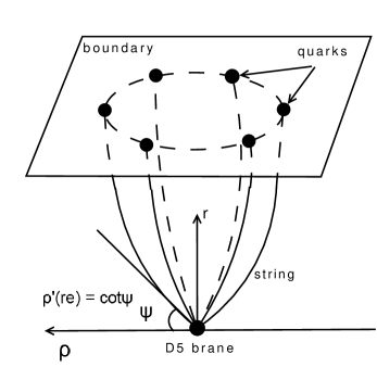
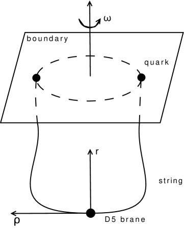
Figure 5.3: String and a brane as the boundary represent a baryon.

On the other hand, a constraint condition, the so-called force balance condition (FBC), in the $r$-direction is also considered

$$\sum_{i=1}^{N_{c}}H^{(i)}\biggr{|}_{r_{e}}=\Sigma\;,$$ (5.68)

with $H$ the Hamilton of the system and

$$\Sigma\equiv\frac{2\pi\alpha^{\prime}}{\mathcal{T}}\frac{\partial S_{D5}}{\partial r_{e}}\;.$$ (5.69)

5.2.2 $\omega$ dependence

From Eq.(5.66), the equation of motion for $\rho(r)$ is obtained

$$\left(\frac{\partial}{\partial\rho}-\frac{\partial}{\partial r}\frac{\partial}{\partial\rho^{\prime}}\right)\mathcal{L}=0\;,$$ (5.70)

where $\mathcal{L}$ is the Lagrangian of the action (5.66).

Substituting Eq.(5.66) into Eq.(5.68) we can obtain the FBC as a boundary condition for the numerical calculations

$$\rho^{\prime}(r_{e})=\frac{R}{r_{e}f(r_{e})^{1/2}}\sqrt{\frac{R^{2}(r_{e}^{4}-r_{0}^{4})r_{e}^{4}}{(r_{e}^{4}+r_{0}^{4})^{2}A^{2}}-1}\;,$$ (5.71)

with

$$A=\frac{1}{N_{c}}\frac{V_{5}}{(2\pi)^{4}(\alpha^{\prime})^{2}}\;.$$

With a given value of $r_{e}$, Eq.(5.70) can be solved with the boundary condition (5.71). The numerical result is shown in Fig. 5.4. The separation distance of quarks with a given $r_{e}$ is

$$l_{q}=2\int_{r_{e}}^{r_{\Lambda}}\rho^{\prime}(r)dr=2\rho(r_{\Lambda})\;.$$ (5.72)

The result of $l_{q}$ as a function of $r_{e}$ is shown in Fig. 5.5. The maximum value of $l_{q}$ is defined as the screening length $l_{s}$ of the baryon $l_{s}$ as shown in Fig. 5.6. We obtain the form of $l_{s}$ as

$$l_{s}=\frac{a}{b\omega+c}-d\;,$$ (5.73)

where it is drawn in Fig. 5.6 with following parameters,

$$l_{s}=\frac{0.51}{0.14\omega+0.22}-0.85\;.$$ (5.74)

In hot QGP, the screening length depends on the temperature and $\omega$ or spin. The smaller screening length of a baryon with higher spin is easier to dissociate. The linear velocity of quarks $v\equiv l_{q}\omega/2$ is similar to Ref. [123] if a drag force in the $x_{3}$ direction orthogonal to the rotating plane is added.

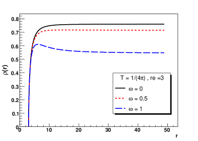
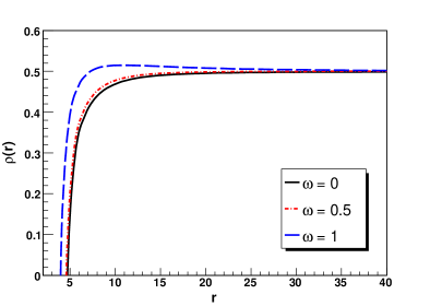
Figure 5.4: Embedding function $\rho(r)$ as a function of $\omega$ with fixed $r_{e}$ (upper plane) and $l_{q}$ with $r_{\Lambda}=100$ (lower plane).

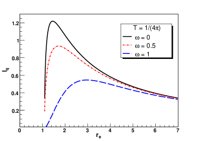
Figure 5.5: Separation distance of quarks as a function of $r_{e}$ with $r_{\Lambda}=100$.

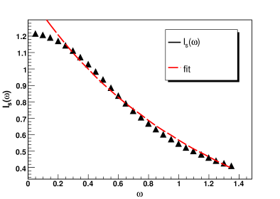
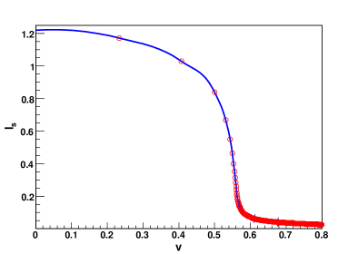
Figure 5.6: Screening length as a function of spin of baryons $\omega$ (upper plane) and linear velocity $v$ (lower plane).

5.2.3 Regge behavior

At the time when the classic string theory was considered as a candidate for the theory of the strong interaction, it was found that the angular momentum of baryons $J$ is proportional to the square of energy $E^{2}$ as follows

$$J\propto E^{2}\;,$$

which is called the Regge behavior. In this model, the angular momentum and energy of the strings read

$$J_{string} = \frac{\partial\mathcal{L}}{\partial\omega}$$ (5.75)

$$= \frac{1}{2\pi\alpha^{\prime}}\int_{r_{e}}^{r_{\Lambda}}dr\frac{\left(\frac{1}{f(r)}+\frac{r^{2}}{R^{2}}\rho^{\prime 2}(r)\right)(\frac{r^{2}}{R^{2}}\rho^{2}\omega)}{\sqrt{-\left(\frac{r^{2}}{R^{2}}\rho^{2}\omega^{2}-f(r)\right)\left(\frac{1}{f(r)}+\frac{r^{2}}{R^{2}}\rho^{\prime 2}(r)\right)}}\;,$$

and

$$E_{string} = \omega\frac{\partial\mathcal{L}}{\partial\omega}-\mathcal{L}$$ (5.76)

$$= \frac{1}{2\pi\alpha^{\prime}}\int_{r_{e}}^{r_{\Lambda}}dr\frac{\left(\frac{1}{f(r)}+\frac{r^{2}}{R^{2}}\rho^{\prime 2}(r)\right)f(r)}{\sqrt{-\left(\frac{r^{2}}{R^{2}}\rho^{2}\omega^{2}-f(r)\right)\left(\frac{1}{f(r)}+\frac{r^{2}}{R^{2}}\rho^{\prime 2}(r)\right)}}\;.$$

The total angular momentum and energy of the system are given by

$$E_{total} = N_{c}E_{string}+E_{brane}\;,$$

$$J_{total} = N_{c}J_{string}+J_{brane}\;,$$ (5.77)

where

$$E_{brane}=\frac{\mathcal{V}(r_{e})V_{5}}{(2\pi)^{5}\alpha^{\prime 3}}\;.$$ (5.78)

The numerical results for $J_{total}$ and $E_{total}$ as functions of $\omega$ with different cutoff $r_{\Lambda}$ are shown in the upper and lower plane of Fig. 5.7, respectively. The relation between $J_{total}$ and $E_{totoal}^{2}$ with the same $\omega$ (i.e. fixed $r_{e}$) is shown in Fig. 5.8. In the case of the same separation distance of quarks, i.e. the fixed value of $l_{q}$, the relation between $J_{total}$ and $E_{totoal}^{2}$ is shown in Fig. 5.9 and 5.10.

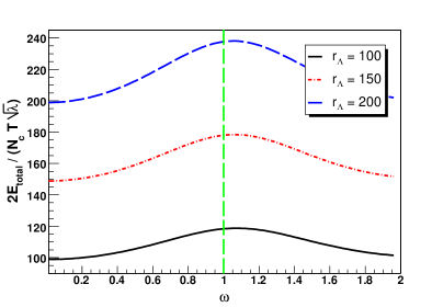
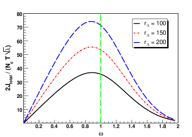
Figure 5.7: $J_{total}$ and $E_{total}$ as functions of $\omega$ with fixed $r_{e}$.

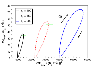
Figure 5.8: The relation between $J_{total}$ and $E_{total}$ with fixed $r_{e}$.

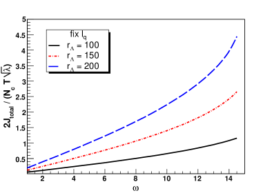
Figure 5.9: $J_{total}$ and $E_{total}$ as functions of $\omega$ with fixed $l_{q}$.

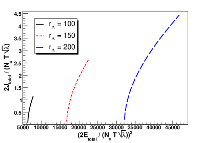
Figure 5.10: The relation between $J_{total}$ and $E_{total}$ with fixed $l_{q}$.

Finally, another physical boundary condition is considered. In order to pick up some configurations for baryons with the same constituents but different $\omega$ or spin, the configurations satisfying the following boundary condition are chosen,

$$\frac{\partial\mathcal{L}}{\partial\rho^{\prime}}=0\;,$$ (5.79)

which gives

$$\frac{1}{4}\>l_{q}^{2}\>\omega^{2}=\left(1-\frac{r_{0}^{4}}{r_{\Lambda}^{4}}\right)\;,$$ (5.80)

or

$$\rho^{\prime}(r_{\Lambda})=0\;.$$ (5.81)

It is observed that the end points of strings move with the speed of light on the cutoff brane with the first condition (5.80), while the string is orthogonal to this brane with the condition (5.81). Unfortunately, it is not guaranteed to find out the points to fulfill the boundary condition (5.80) for small $\omega$. The configurations for the strings fulfilling with condition (5.81) are shown in Fig. 5.11.

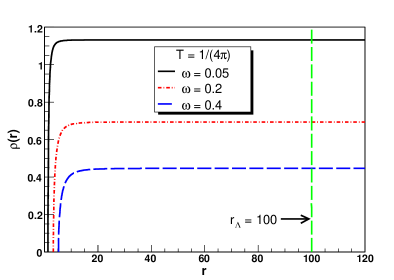
Figure 5.11: Embedding function $\rho(r)$ with orthogonal boundary condition (5.81).

In this case, the FBC in the $\rho$-direction becomes

$$\frac{\partial E_{I}}{\partial\rho}=m_{q}\omega^{2}\rho\;,$$ (5.82)

with $m_{q}=\frac{1}{2\pi\alpha^{\prime}}(r_{\Lambda}-r_{0})$ the mass of quarks and $E_{I}$ the interaction potential defined as

$$E_{I}=N_{c}E_{string}-E_{q}+E_{brane}\;,$$ (5.83)

where

$$E_{q}=\frac{N_{c}}{2\pi\alpha^{\prime}}\int_{r_{0}}^{r_{\Lambda}}dr\;,$$ (5.84)

is the energy of free quarks. The $\omega$ dependence of angular momentum and energy with the FBC (5.82) is shown in Fig. 5.12. The relation between $J_{total}$ and $E_{totoal}^{2}$ with the FBC (5.82) is shown in Fig. 5.13.

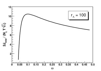
Figure 5.12: Angular momentum and energy with the FBC (5.82) as functions of $\omega$.

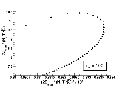
Figure 5.13: Angular momentum and energy with the FBC (5.82) as functions of $\omega$.

5.2.4 Conclusion

We calculate the $\omega$ dependence of the baryon screening length in strongly coupled hot plasma via AdS/CFT duality. In our model, we consider a baryon in the bulk space as a probe and a baryon at the boundary with high spin using the rotating strings. We obtain the $\omega$ dependence of the embedding function of these strings and their screening length. We also investigate the relation between total angular momentum and energy of baryons and show the numerical results in three different conditions. We find that these solutions with orthogonal boundary condition (5.82) are the best candidates for baryons with same constituents but different spins.

Chapter 6 Fluid dynamics with triangle anomaly

The RHIC data for collective flows have been well described by the ideal and dissipative hydrodynamics [47, 50, 105, 204, 205, 206, 207, 208]. The correspondence of relativistic hydrodynamics to charged black-branes was investigated by AdS/CFT duality [146, 145]. A new term associated with the axial anomalies was found in the first order dissipative hydrodynamics (see, e.g., Ref. [147] about holographic hydrodynamics with multiple/non-Abelian symmetries, or Ref. [148] in Sakai-Sugimoto model). Recently the new term has been derived in hydrodynamics with a triangle anomaly [149]. A similar result was also obtained in microscopic theory of the superfluid [150]. This problem is closely related to the so-called Chiral Magnetic Effect (CME) in heavy ion collisions [151, 152, 153, 154]. When two energetic nuclei pass each other a strong magnetic field up to $10^{18}$ G is formed, which breaks local parity via axial anomaly. This effect may be observed through charge separation. Hydrodynamics in an external background field can be used to pin down the CME in real time simulation. However the anomalous term in the charge current breaks the second law of thermodynamics unless new terms of vorticity and magnetic field are introduced in the charge and entropy currents [149].

In this chapter, we try to provide a consistent description of the kinetic equation with a triangle anomaly. We will derive the kinetic equation to the next to leading order as well as the leading order correction to the particle distribution function arising from anomaly. These results are compatible with the entropy principle of the second law of thermodynamics and the charge/energy-momentum conservation equations. Most of the contents in this chapter are taken from Ref. [209]

6.1 Constraining distribution function with anomaly compatible to second law of thermodynamics

In this and the next sections we will consider the most simple case with one charge and one particle species (without anti-particles). The relativistic Boltzmann equation for the on-shell phase-space distribution $f(x,p)$ in a background electromagnetic field $F_{\mu\nu}$ is given by Eq.(4.1). Note that $\mathcal{C}[f]$ contains a normal collision term $\mathcal{C}_{0}[f]$ and a source term from anomaly $\mathcal{C}_{A}[f]$, $\mathcal{C}[f]=\mathcal{C}_{0}[f]+\mathcal{C}_{A}[f]$. We assume that $\mathcal{C}_{A}[f]$ is at most of the first order, a small quantity. The necessity for the source term is to make the charge conservation equation hold,

$$\partial_{\mu}j^{\mu}=-CE^{\mu}B_{\mu}\equiv-CE\cdot B.$$ (6.1)

Here $j^{\mu}$ is the charge current and $E^{\mu}=u_{\nu}F^{\mu\nu}$ and $B_{\mu}=\frac{1}{2}\epsilon_{\mu\nu\alpha\beta}u^{\nu}F^{\alpha\beta}$ are electric and magnetic field vectors respectively, where $u_{\mu}$ is the fluid velocity and $\epsilon_{\mu\nu\alpha\beta}=-\epsilon^{\mu\nu\alpha\beta}=-1,1$ for the order of Lorentz indices $(\mu\nu\alpha\beta)$ is an even/odd permutation of $(0123)$. However, the presence of the source term should not influence the energy momentum conservation,

$$\partial_{\mu}T^{\mu\nu}=F^{\nu\mu}j_{\mu}.$$ (6.2)

One can verify that the equilibrium solution of the distribution function,

$$f_{0}=\frac{1}{\exp[\beta u_{\mu}(p^{\mu}-QF^{\mu\nu}x_{\nu})-\beta Q\mu_{0}]-e},$$ (6.3)

satisfies the collisionless Boltzmann equation (4.1) in an external field for constant $\beta=1/T$ ($T$ is the local temperature), $u_{\mu}$ and $\mu_{0}$ (local chemical potential without electromagnetic field). Here $e=0,\pm 1$ for Boltzmann, Bose and Fermi distributions respectively. When $\beta$, $u_{\mu}$ and $\mu_{0}$ are not constants but functions of space-time, the Boltzmann equation (4.1) is not satisfied automatically. Note that we can absorb $-Qx_{\nu}u_{\mu}F^{\mu\nu}=Qx\cdot E$ into $\mu_{0}$ so that $f_{0}$ has the form of an equilibrium distribution function,

$$f_{0}(x,p) = \frac{1}{e^{(u\cdot p-Q\mu)/T}-e},$$ (6.4)

where $\mu\equiv\mu_{0}-x\cdot E$.

We assume that the distribution function $f$ in presence of an anomaly is a solution of the Boltzmann equation with collision terms in Eq. (4.1), where $\beta$, $u_{\mu}$ and $\mu$ are functions of space-time. Generally $f(x,p)$ can be written in the following form,

$$f(x,p) = \frac{1}{e^{(u\cdot p-Q\mu)/T+\chi(x,p)}-e}=f_{0}(x,p)+f_{1}(x,p),$$ (6.5)

where $f_{0}(x,p)$ is given in Eq. (6.4) and $f_{1}(x,p)$ is the first order deviation from it,

$$f_{1}(x,p) = -f_{0}(x,p)\left[1+ef_{0}(x,p)\right]\chi(x,p).$$ (6.6)

It is known that a magnetic field is closely related to a charge rotation characterized by vorticity. So we introduce into the distribution function terms associated with the vorticity-induced current $\omega_{\mu}=\frac{1}{2}\epsilon_{\mu\nu\alpha\beta}u^{\nu}\partial^{\alpha}u^{\beta}$ and the magnetic field 4-vector $B_{\mu}$ which are assumed to be of the first order, which provide a leading order correction to the particle distribution function. For simplicity we will neglect viscous and diffusive effects throughout the paper, then the ordinary form in the current scheme for $\chi(x,p)$ reads,

$$\chi(x,p) = \lambda(p)p\cdot\omega+\lambda_{B}(p)p\cdot B,$$ (6.7)

where $\lambda(p)$ and $\lambda_{B}(p)$ are functions of $\mu$, $T$, and $u\cdot p$ and have mass dimension $-2$ and $-3$ respectively. We will show that $\lambda(p)$ and $\lambda_{B}(p)$ must depend on momentum otherwise they will contradict the entropy principle from the second law of thermodynamics.

Using Eq. (6.5) we can decompose the charge and entropy currents and the stress tensor into equilibrium values and the leading order (first order) corrections as $j^{\mu}=j_{0}^{\mu}+j_{1}^{\mu}$, $S^{\mu}=S_{0}^{\mu}+S_{1}^{\mu}$ and $T^{\mu\nu}=T_{0}^{\mu\nu}+T_{1}^{\mu\nu}$ with

$$j_{0,1}^{\mu}(x) = q\int[dp]p^{\mu}f_{0,1}(x,p),$$

$$S_{0}^{\mu}(x) = -\int[dp]p^{\mu}\psi(f_{0}),$$

$$S_{1}^{\mu}(x) = -\int[dp]p^{\mu}\psi^{\prime}(f_{0})f_{1},$$

$$T_{0,1}^{\mu\nu}(x) = \int[dp]p^{\mu}p^{\nu}f_{0,1}(x,p),$$ (6.8)

where we have defined $[dp]\equiv d_{g}\frac{d^{3}p}{(2\pi)^{3}(u\cdot p)}$ ($d_{g}$ is the degeneracy factor), $\psi(f_{0})=f_{0}\ln(f_{0})-e(1+ef_{0})\ln(1+ef_{0})$ and $\psi^{\prime}(f_{0})=\ln[f_{0}/(1+ef_{0})]=-(u\cdot p-Q\mu)/T$. Inserting $f_{0}$ into the above formula, we obtain the charge and entropy currents and the stress tensor in equilibrium, $j_{0}^{\mu}=nu^{\mu}$, $S_{0}^{\mu}=su^{\mu}$ and $T_{0}^{\mu\nu}=(\epsilon+P)u^{\mu}u^{\nu}-Pg^{\mu\nu}$, with the energy density $\varepsilon$, the pressure $P$, the particle number density $n$ and the entropy density $s=(\epsilon+P-n\mu)/T$. Using Eqs. (6.6,6.7,6.8), we obtain

$$j_{1}^{\mu} = \xi\omega^{\mu}+\xi_{B}B^{\mu},$$

$$T_{1}^{\mu\nu} = DT\left(u^{\mu}\omega^{\nu}+u^{\nu}\omega^{\mu}\right)+D_{B}T\left(u^{\mu}B^{\nu}+u^{\nu}B^{\mu}\right),$$

$$S_{1}^{\mu} = -\frac{\mu}{T}(\xi\omega^{\mu}+\xi_{B}B^{\mu})+(D\omega^{\mu}+D_{B}B^{\mu}),$$ (6.9)

where

$$\xi = -QJ_{21}^{\lambda}\equiv\frac{1}{3}Q\int[dp][(p\cdot u)^{2}-m^{2}]f_{0}(1+ef_{0})\lambda(p),$$

$$\xi_{B} = -QJ_{21}^{\lambda_{B}}\equiv\frac{1}{3}Q\int[dp][(p\cdot u)^{2}-m^{2}]f_{0}(1+ef_{0})\lambda_{B}(p),$$

$$D = -\frac{J_{31}^{\lambda}}{T}\equiv\frac{1}{3T}\int[dp][(p\cdot u)^{2}-m^{2}](p\cdot u)f_{0}(1+ef_{0})\lambda(p),$$

$$D_{B} = -\frac{J_{31}^{\lambda_{B}}}{T}\equiv\frac{1}{3T}\int[dp][(p\cdot u)^{2}-m^{2}](p\cdot u)f_{0}(1+ef_{0})\lambda_{B}(p).$$ (6.10)

On the other hand, $\xi$, $\xi_{B}$, $D$ and $D_{B}$ as functions of $\mu$ and $T$ can be determined by the second law of thermodynamics or the entropy principle together with Eq. (6.1-6.2). The entropy production rate is given by

$$\partial_{\mu}\left(su^{\mu}-\frac{\mu}{T}\nu^{\mu}\right) = \frac{\pi^{\mu\nu}}{T}\partial_{\mu}u_{\nu}-\nu^{\mu}\left(\partial_{\mu}\frac{\mu}{T}+\frac{E^{\mu}}{T}\right)-C\frac{\mu}{T}E\cdot B\;,$$ (6.11)

where $C$ is a constant whose sign is arbitrary. We find that $\partial_{\mu}(su^{\mu}+S_{1}^{\mu})$ cannot be positive definite unless we make a shift to introduce a new entropy current $\tilde{S}^{\mu}$ as follows,

$$\tilde{S}^{\mu} = su^{\mu}+S_{1}^{\mu}-(D\omega^{\mu}+D_{B}B^{\mu})=su^{\mu}-\frac{\mu}{T}\left(\xi\omega^{\mu}+\xi_{B}B^{\mu}\right)$$ (6.12)

$$= \frac{1}{T}(Pu^{\mu}-\mu j^{\mu}+u_{\lambda}T^{\lambda\mu})-(D\omega^{\mu}+D_{B}B^{\mu})$$

We will use the thermodynamic relation

$$\partial_{\mu}(Pu^{\mu})=j_{0}^{\mu}\partial_{\mu}\overline{\mu}-T_{0}^{\lambda\mu}\partial_{\mu}u_{\lambda}$$ (6.13)

and the identities

$$u^{\mu}u^{\lambda}\partial_{\mu}\omega_{\lambda} = \frac{1}{2}\partial_{\mu}\omega^{\mu},$$

$$u^{\mu}u^{\lambda}\partial_{\mu}B_{\lambda} = \partial_{\mu}B^{\mu}-2\omega^{\rho}E_{\rho},$$

$$\partial_{\mu}\omega^{\mu} = -\frac{2}{\epsilon+P}(n\omega^{\mu}E_{\mu}+\omega^{\mu}\partial_{\mu}P),$$

$$\partial_{\mu}B^{\mu} = 2\omega^{\rho}E_{\rho}-\frac{1}{\epsilon+P}(nB_{\lambda}E^{\lambda}+B^{\mu}\partial_{\mu}P),$$ (6.14)

to evaluate $\partial_{\mu}\tilde{S}^{\mu}$. We have used the shorthand notation $\overline{\mu}\equiv\mu/T$ in Eq. (6.13). Following the same procedure as in Ref. [149], we obtain

$$\partial_{\mu}\widetilde{S}^{\mu} = \omega^{\mu}\left[\xi^{SS}\partial_{\mu}\overline{\mu}-\partial_{\mu}D+\frac{2D}{\epsilon+P}\partial_{\mu}P\right]$$ (6.15)

$$+B^{\mu}\left[\xi_{B}^{SS}\partial_{\mu}\overline{\mu}-\partial_{\mu}D_{B}+\frac{D_{B}}{\epsilon+P}\partial_{\mu}P\right]$$

$$+E\cdot\omega\left[\frac{1}{T}\xi^{SS}+\frac{2nD}{\epsilon+P}-2D_{B}\right]$$

$$+E\cdot B\left[\frac{1}{T}\xi_{B}^{SS}+C\frac{\mu_{A}}{T}+\frac{nD_{B}}{\epsilon+P}\right].$$

where we have defined

$$\xi^{SS} = \frac{DTn}{\epsilon+P}-\xi,\;\xi_{B}^{SS}=\frac{D_{B}Tn}{\epsilon+P}-\xi_{B}.$$ (6.16)

For the constraint $\partial_{\mu}\widetilde{S}^{\mu}\geq 0$ to hold, we impose that all quantities inside the square brackets should vanish. We finally obtain

$$D=\frac{1}{3}C\frac{\mu^{3}}{T},\;D_{B}=\frac{1}{2}C\frac{\mu^{2}}{T},\;\xi=-C\frac{sT\mu^{2}}{\epsilon+P},\;\xi_{B}=-C\frac{sT\mu}{\epsilon+P}.$$ (6.17)

Using Eqs. (6.16,6.17), one can verify that the values of $\xi^{SS}$ and $\xi_{B}^{SS}$ are identical to Ref. [149]. The difference between our values in Eq. (6.17) and those in Ref. [149] arises from the fact that we do not use the Landau frame while the authors of Ref. [149] do. By equating Eq. (6.10) and (6.17), we obtain equations for $\lambda$ and $\lambda_{B}$,

$$QJ_{21}^{\lambda}=-\xi,\;J_{31}^{\lambda}=-DT,\;QJ_{21}^{\lambda_{B}}=-\xi_{B},\;J_{31}^{\lambda_{B}}=-D_{B}T.$$ (6.18)

Equation (6.18) forms a complete set of constraints for $\lambda$ and $\lambda_{B}$. We note that $\lambda$ and $\lambda_{B}$ must depend on momentum in general. If $\lambda$ and $\lambda_{B}$ are constants, we would obtain

$$\frac{\xi}{DT}=\frac{\xi_{B}}{D_{B}T}=Q\frac{J_{21}}{J_{31}},$$ (6.19)

which contradict Eq. (6.17) from the entropy principle.

We can expand $\lambda(p)$ and $\lambda_{B}(p)$ in powers of $u\cdot p$,

$$\lambda(p)=\sum_{i=0}\lambda_{i}(u\cdot p)^{i},\;\lambda_{B}(p)=\sum_{i=0}\lambda_{i}^{B}(u\cdot p)^{i}.$$ (6.20)

So we obtain the following expressions

$$J_{n1}^{\lambda}=\sum_{i=0}\lambda_{i}J_{i+n,1},\;J_{n1}^{\lambda_{B}}=\sum_{i=0}\lambda_{i}^{B}J_{i+n,1},$$ (6.21)

for $n=2,3$. Here the functions $J_{nq}$ are integrals defined in Ref. [46, 205],

$$J_{nq}=(-1)^{q}\frac{1}{(2q+1)!!}\int\frac{d^{3}p}{(2\pi)^{3}(u\cdot p)}[(u\cdot p)^{2}-m^{2}]^{q}(u\cdot p)^{n-2q}f_{0}(1+ef_{0}),$$ (6.22)

Using Eqs. (6.20,6.21) in Eq. (6.18), we can constrain the coefficients $\lambda_{i}$ and $\lambda_{i}^{B}$. If we expand both $\lambda(p)$ and $\lambda_{B}(p)$ to the first power of $u\cdot p$, we can completely fix the coefficients $\lambda_{0,1}$ and $\lambda_{0,1}^{B}$ from Eq. (6.18) since we have two equations for $\lambda_{0,1}$ and two for $\lambda_{0,1}^{B}$,

$$\left(\begin{array}[]{cc}QJ_{21}&QJ_{31}\\ J_{31}&J_{41}\end{array}\right)\left(\begin{array}[]{c}\lambda_{0}\\ \lambda_{1}\end{array}\right) = \left(\begin{array}[]{c}-\xi\\ -DT\end{array}\right),$$ (6.29)

whose solutions to $\lambda_{0,1}$ are

$$\left(\begin{array}[]{c}\lambda_{0}\\ \lambda_{1}\end{array}\right) = \frac{1}{Q(J_{21}J_{41}-J_{31}^{2})}\left(\begin{array}[]{c}-\xi J_{41}+DTQJ_{31}\\ \xi J_{31}-DTQJ_{21}\end{array}\right).$$ (6.34)

The equations and solutions for $\lambda_{0,1}^{B}$ are in the same form as Eqs. (6.29,6.34) with replacements $\lambda_{0,1}\rightarrow\lambda_{0,1}^{B}$, $\xi\rightarrow\xi_{B}$ and $D\rightarrow D_{B}$.

In massless limit, the integrals of $J_{nk}$ are well defined as the Poly logarithm functions $\textrm{Li}_{n}(z)$,

$$-\textrm{Li}_{s}(-z)=\frac{1}{\Gamma(s)}\int_{0}^{\infty}\frac{t^{s-1}}{e^{t}/z+1}dt.\quad\textrm{execpt for }z\leq-1$$ (6.35)

When $\mu$ is small, the Poly logarithm functions can be expanded in $\frac{\mu}{T}$, so the leading order contribution of the solution (6.34) is then

$$\lambda_{0}\approx-CG_{1}\frac{\mu^{2}}{T^{4}}\;, \lambda_{1}\approx CG_{2}\frac{\mu^{2}}{T^{5}}\;,$$

$$\lambda_{0}^{B}\approx\frac{\lambda}{\mu}\;, \lambda_{1}^{B}\approx\frac{\lambda_{1}}{\mu}\;,$$ (6.36)

where $G_{1}$ and $G_{2}$ are two constants, $G_{1}\equiv 607500\pi^{2}\zeta(5)/(d_{g}G_{0})$ and $G_{2}\equiv 1260\pi^{6}/(d_{g}G_{0})$ with $G_{0}\equiv 455625\zeta(3)\zeta(5)-49\pi^{8}$. We notice that the $D$ terms in Eq. (6.34) are negligible, so the solutions are proportional to $\xi$.

6.2 One charge with particle/anti-particle

We now consider one charge case but add anti-particles to the system. We will calculate $\lambda(p)$ and $\lambda_{B}(p)$. Since there are particles and anti-particles, we recover the index $Q=\pm 1$ in particle distribution function, $f\rightarrow f^{Q}$ and $f_{0,1}\rightarrow f_{0,1}^{Q}$. In Eq. (6.8), summations over $Q$ should be added. In Eq. (6.10) we also have to add the index $Q$ to $J_{n1}^{\lambda}$ and $J_{n1}^{\lambda_{B}}$: $J_{n1}^{\lambda}\rightarrow J_{n1}^{\lambda,Q}$ and $J_{n1}^{\lambda_{B}}\rightarrow J_{n1}^{\lambda_{B},Q}$ ($n=2,3$), and add summations over $Q$ into the formula of $\xi$, $\xi_{B}$, $D$, $D_{B}$. Inserting $f_{0}^{Q}$ into Eq. (6.8), we obtain the charge and entropy currents and the stress tensor in equilibrium, $j_{0}^{\mu}=nu^{\mu}$, $S_{0}^{\mu}=su^{\mu}$ and $T_{0}^{\mu\nu}=(\epsilon+P)u^{\mu}u^{\nu}-Pg^{\mu\nu}$, with the particle number density $n\equiv\sum_{Q}Qn_{Q}$, the energy density $\epsilon=\sum_{Q}\epsilon_{Q}$, the pressure $P=\sum_{Q}P_{Q}$, and the entropy density $s=\sum_{Q}s_{Q}=(\epsilon+P-n\mu)/T$. The solutions to $\xi,\xi_{B},D,D_{B}$ are the same as in Eq. (6.17). Then Eq. (6.18) is modified to

$$J_{21}^{\lambda,+}-J_{21}^{\lambda,-}=-\xi,\;J_{31}^{\lambda,+}+J_{31}^{\lambda,+}=-DT,$$

$$J_{21}^{\lambda_{B},+}-J_{21}^{\lambda_{B},-}=-\xi_{B},\;J_{31}^{\lambda_{B},+}+J_{31}^{\lambda_{B},-}=-D_{B}T.$$ (6.37)

Eq. (6.21) now becomes

$$J_{n1}^{\lambda,Q}=\sum_{i=0}\lambda_{i}J_{i+n,1}^{Q},\;J_{n1}^{\lambda_{B},Q}=\sum_{i=0}\lambda_{i}^{B}J_{i+n,1}^{Q},$$ (6.38)

In the case of minimal number of coefficients we can completely fix the coefficients $\lambda_{0,1}$ by solving following system of equations,

$$\left(\begin{array}[]{cc}\delta J_{21}&\delta J_{31}\\ \sigma J_{31}&\sigma J_{41}\end{array}\right)\left(\begin{array}[]{c}\lambda_{0}\\ \lambda_{1}\end{array}\right) = \left(\begin{array}[]{c}-\xi\\ -DT\end{array}\right),$$ (6.45)

where we have used the shorthand notation, $\delta J_{n1}\equiv J_{n1}^{+}-J_{n1}^{-}$ and $\sigma J_{n1}\equiv J_{n1}^{+}+J_{n1}^{-}$. The solutions to $\lambda_{0,1}$ are

$$\left(\begin{array}[]{c}\lambda_{0}\\ \lambda_{1}\end{array}\right) = \frac{1}{\Delta}\left(\begin{array}[]{c}-\xi(\sigma J_{41})+DT(\delta J_{31})\\ \xi(\sigma J_{31})-DT(\delta J_{21})\end{array}\right),$$ (6.50)

where $\Delta=(\delta J_{21})(\sigma J_{41})-(\sigma J_{31})(\delta J_{31})$. The equations and solutions for $\lambda_{0,1}^{B}$ are in the same form as Eqs. (6.45,6.50) with replacements $\lambda_{0,1}\rightarrow\lambda_{0,1}^{B}$, $\xi\rightarrow\xi_{B}$ and $D\rightarrow D_{B}$.

Using integration by parts in Appendix B, $\delta J_{nk}$ and $\sigma J_{nk}$ for $n=2,3,4$ and $k=1$ are given by

$$\delta J_{21}=\frac{d_{g}T^{4}}{6}\left(\bar{\mu}+\frac{\bar{\mu}^{3}}{\pi^{2}}\right)\;, \sigma J_{21}=\frac{d_{g}T^{4}}{\pi^{2}}\left[-\textrm{Li}_{3}(-e^{\bar{\mu}})-\textrm{Li}_{3}(-e^{-\bar{\mu}})\right]\;$$

$$\delta J_{31}=\frac{4d_{g}T^{5}}{\pi^{2}}\left[-\textrm{Li}_{4}(-e^{\bar{\mu}})-\textrm{Li}_{4}(-e^{-\bar{\mu}})\right]\;, \sigma J_{31}=d_{g}T^{5}\left[\frac{7\pi^{2}}{90}+\frac{\bar{\mu}^{2}}{3}+\frac{\bar{\mu}^{4}}{6\pi^{2}}\right]\;$$

$$\delta J_{41}=d_{g}T^{6}\left[\frac{7\pi^{2}}{18}\bar{\mu}+\frac{5}{9}\bar{\mu}^{3}+\frac{\bar{\mu}^{5}}{6\pi^{2}}\right]\;, \sigma J_{41}=\frac{20d_{g}T^{6}}{\pi^{2}}\left[-\textrm{Li}_{5}(-e^{\bar{\mu}})-\textrm{Li}_{5}(-e^{-\bar{\mu}})\right]\;.$$ (6.51)

For massless fermions and small $\overline{\mu}$, we have,

$$\sigma J_{21} \approx 9\zeta(3)G,\;\sigma J_{31}\approx\frac{7\pi^{4}}{15}GT,\;\sigma J_{41}\approx 225\zeta(5)GT^{2},$$

$$\delta J_{21} \approx \pi^{2}\overline{\mu}G,\;\delta J_{31}\approx 36\zeta(3)\overline{\mu}GT,\;\delta J_{41}\approx\frac{7\pi^{4}}{3}\overline{\mu}GT^{2},$$

$$\Delta \approx \frac{\pi^{2}}{5}G^{2}G_{0}T^{2}\overline{\mu}.$$ (6.52)

where $G\equiv\frac{d_{g}T^{4}}{6\pi^{2}}$ and $G_{0}\equiv-84\pi^{2}\zeta(3)+1125\zeta(5)$. The solutions have very simple form,

$$\lambda_{0}\approx CG_{1}\frac{\mu}{T^{3}}\;, \lambda_{1}\approx-CG_{2}\frac{\mu}{T^{4}}\;,$$

$$\lambda_{0}^{B}\approx\frac{\lambda}{\mu}\;, \lambda_{1}^{B}\approx\frac{\lambda_{1}}{\mu}\;,$$ (6.53)

where we have used two constants, $G_{1}\equiv\frac{6750\pi^{2}\zeta(5)}{d_{g}G_{0}}$, $G_{2}\equiv\frac{14}{d_{g}G_{0}}$. We notice that the $D$ terms in Eq. (6.50) are negligible, so the solutions are proportional to $\xi$. Note that the quantity $\frac{n\mu}{\epsilon+P}\sim\overline{\mu}^{2}$ is also small and we have dropped it, since $n\mu\approx\frac{d_{g}}{6\pi^{2}}T^{4}\overline{\mu}^{2}$ and $\epsilon+P=\frac{4}{3}\epsilon\approx d_{g}\frac{7\pi^{2}}{90}T^{4}$.

6.3 With two charges and particle/antiparticle

As an example for the case of two charges, we consider adding to the system the chirality or an axial $U(1)$ charge to particles. Then there are two currents, one for each chirality, or equivalently, for the $U(1)/U_{A}(1)$ charge. For simplicity we assume that there is an anomaly for the axial charge current but no anomaly for the charge one. There are distribution functions for right-hand and left-hand particles, $f_{a}^{Q}(x,p)$ ($a=R,L$), with chemical potentials $\mu_{R.L}=\mu\pm\mu_{A}$. As an extension to Eq. (6.7), the corrections $\chi_{a}(x,p)$ in $f_{a}^{Q}(x,p)$ are now $\chi_{a}(x,p)=\lambda_{a}p^{\mu}\omega_{\mu}+\lambda_{aB}p^{\mu}B_{\mu}$. Instead of right-hand and left-hand quantities $X_{a}$, we can equivalently use $X=X_{R}+X_{L}$ and $X_{A}=X_{R}-X_{L}$, where $X=\lambda,\lambda_{B},\xi,\xi_{B},n,s,\epsilon,P,j_{\mu}$. The distribution functions $f_{a}^{Q}(x,p)$ satisfy two separate Boltzmann equations of the following form,

$$p^{\mu}\left(\frac{\partial}{\partial x^{\mu}}-QF_{\mu\nu}\frac{\partial}{\partial p_{\nu}}\right)f_{a}^{Q}(x,p)=\mathcal{C}_{aQ}[f_{b}^{Q^{\prime}}].$$ (6.54)

The $U(1)/U_{A}(1)$ charge and entropy currents and the stress tensor in equilibrium are give by: $j_{0}^{\mu}=nu^{\mu}$, $j_{A0}^{\mu}=n_{A}u^{\mu}$, $S_{0}^{\mu}=su^{\mu}$ and $T_{0}^{\mu\nu}=(\epsilon+P)u^{\mu}u^{\nu}-Pg^{\mu\nu}$, with the particle number density $n\equiv\sum_{aQ}Qn_{aQ}$ ($a=R,L$; $Q=\pm 1$), the energy density $\epsilon=\sum_{aQ}\epsilon_{aQ}$, the pressure $P=\sum_{aQ}P_{aQ}$, and the entropy density $s=\sum_{aQ}s_{aQ}=(\epsilon+P-\sum_{a}n_{a}\mu_{a})/T$.

Similar to Eqs. (6.68,6.70), the $U(1)/U_{A}(1)$ charge conservation equations (6.1) can be derived as

$$\partial_{\mu}j^{\mu}(x) = \int[dp](\mathcal{C}_{R,+}-\mathcal{C}_{R,+}+\mathcal{C}_{L,+}-\mathcal{C}_{L,+})=0,$$ (6.55)

$$\partial_{\mu}j_{A}^{\mu}(x) = \int[dp](\mathcal{C}_{R,+}-\mathcal{C}_{R,-}-\mathcal{C}_{L,+}+\mathcal{C}_{L,+})=-CE^{\mu}B_{\mu},$$ (6.56)

where we have used Eq. (6.69). The energy and momentum conservation equation reads,

$$\partial_{\mu}T^{\mu\nu}-F^{\nu\mu}j_{\mu} = \int[dp]p^{\nu}(\mathcal{C}_{R,+}+\mathcal{C}_{R,-}+\mathcal{C}_{L,+}+\mathcal{C}_{L,-})=0,$$ (6.57)

where we have used Eq. (6.72).

Similar to Eq. (6.10), we can express $\xi_{a}$, $\xi_{aB}$, $D$ and $D_{B}$ in terms of $\lambda_{a}$ and $\lambda_{aB}$ as,

$$\xi_{a}=-(J_{21}^{\lambda_{a},+}-J_{21}^{\lambda_{a},-}),\;\;-DT=J_{31}^{\lambda_{R},+}+J_{31}^{\lambda_{R},-}+J_{31}^{\lambda_{L},+}+J_{31}^{\lambda_{L},-},$$

$$\xi_{aB}=-(J_{21}^{\lambda_{aB},+}-J_{21}^{\lambda_{aB},-}),\;\;-D_{B}T=J_{31}^{\lambda_{RB},+}+J_{31}^{\lambda_{RB},-}+J_{31}^{\lambda_{LB},+}+J_{31}^{\lambda_{LB},-},$$ (6.58)

for $a=R,L$. We have the following first order corrections,

$$j_{1}^{\mu} = j_{R1}^{\mu}+j_{L1}^{\mu}=\sum_{a=R,L}(\xi_{a}\omega^{\mu}+\xi_{aB}B^{\mu})=\xi\omega^{\mu}+\xi_{B}B^{\mu},$$

$$j_{A1}^{\mu} = j_{R1}^{\mu}-j_{L1}^{\mu}=(\xi_{R}-\xi_{L})\omega^{\mu}+(\xi_{RB}-\xi_{LB})B^{\mu}=\xi_{A}\omega^{\mu}+\xi_{AB}B^{\mu},$$

$$T_{1}^{\mu\nu} = DT\left(u^{\mu}\omega^{\nu}+u^{\nu}\omega^{\mu}\right)+D_{B}T\left(u^{\mu}B^{\nu}+u^{\nu}B^{\mu}\right),$$

$$S_{1}^{\mu} = -\sum_{a=R,L}\frac{\mu_{a}}{T}(\xi_{a}\omega^{\mu}+\xi_{aB}B^{\mu})+(D\omega^{\mu}+D_{B}B^{\mu})$$ (6.59)

$$= -\sum_{i=\mathrm{null},A}\frac{\mu_{i}}{T}(\xi_{i}\omega^{\mu}+\xi_{iB}B^{\mu})+(D\omega^{\mu}+D_{B}B^{\mu}).$$

It can be verified that the entropy current in Eq. (6.59) cannot satisfy $\partial_{\mu}S^{\mu}\geq 0$ unless $C=0$. In order to ensure the positivity of $\partial_{\mu}S^{\mu}$ in presence of an anomaly, one would have to substract the vector $Q^{\mu}=D\omega^{\mu}+D_{B}B^{\mu}$ from $S^{\mu}$. With $U(1)$ and $U_{A}(1)$ charges, we have

$$\widetilde{S}^{\mu} = S^{\mu}-Q^{\mu}=su^{\mu}-\sum_{a=R,L}\overline{\mu}_{a}(\xi_{a}\omega^{\mu}+\xi_{aB}B^{\mu})$$ (6.60)

$$= \frac{1}{T}(Pu^{\mu}-\sum_{a=R,L}\mu_{a}j_{a}^{\mu}+u_{\lambda}T^{\lambda\mu})-Q^{\mu}.$$

In the same way as in Sec. 6.1, the divergence of the entropy current can be evaluated as,

$$\partial_{\mu}\widetilde{S}^{\mu} = \omega^{\mu}\left[\sum_{a=R,L}\partial_{\mu}\overline{\mu}_{a}\left(\frac{n_{i}TD}{\epsilon+P}-\xi_{a}\right)-\partial_{\mu}D+\frac{2D}{\epsilon+P}\partial_{\mu}P\right]$$ (6.61)

$$+B^{\mu}\left[\sum_{a=R,L}\partial_{\mu}\overline{\mu}_{a}\left(\frac{n_{i}TD_{B}}{\epsilon+P}-\xi_{aB}\right)-\partial_{\mu}D_{B}+\frac{D_{B}}{\epsilon+P}\partial_{\mu}P\right]$$

$$+E\cdot\omega\left[\sum_{a=R,L}\left(\frac{n_{a}D}{\epsilon+P}-\frac{\xi_{a}}{T}\right)+\frac{2nD}{\epsilon+P}-2D_{B}\right]$$

$$+E\cdot B\left[\sum_{a=R,L}\left(\frac{n_{a}D_{B}}{\epsilon+P}-\frac{\xi_{aB}}{T}\right)+C\frac{\mu_{A}}{T}+\frac{nD_{B}}{\epsilon+P}\right],$$

following Eqs. (6.55-(6.57)). By imposing all quantities inside the square brackets to vanish we can solve $\xi_{a}$, $\xi_{aB}$, $D$, $D_{B}$ as follows,

$$D =-C\mu_{A}T\;, D_{B}=-C\mu_{A}\overline{\mu}\;,$$

$$\xi =-2C\mu\mu_{A}\left(1-\frac{n\mu}{\epsilon+P}\right)\;, \xi_{A}=-C\mu^{2}\left(1-\frac{2n_{A}\mu_{A}}{\epsilon+P}\right)\;,$$

$$\xi_{B} =-C\mu_{A}\left(1-\frac{n\mu}{\epsilon+P}\right)\;, \xi_{AB}=-C\mu\left(1-\frac{n_{A}\mu_{A}}{\epsilon+P}\right)\;,$$ (6.62)

In small $\mu_{A}$ limit, Eq.(6.62) will be

$$D=-C\mu_{A}T\;, \quad\xi=-2C\mu\mu_{A}\;, \quad\xi_{B}=-C\mu_{A}\;,$$

$$D_{B}=-C\mu_{A}\overline{\mu}, \quad\xi_{A}=-C\mu^{2}\;, \quad\xi_{AB}=-C\mu\;,$$ (6.63)

which is identical to the result of Ref. [152, 154]. Here we have assumed that all integral constants are vanishing. Note that Eq. (6.63) is the result of the entropy principle in the hydrodynamic approach which was also obtained in Ref. [210, 211, 212].

Equivalently we can use $\xi_{R}=(\xi+\xi_{A})/2$ and $\xi_{L}=(\xi-\xi_{A})/2$ to determine $\lambda_{a}$, $\lambda_{aB}$ $(a=R,L)$ via solving a system of equations (6.58), where the first/second line (each has three equations) is for $\lambda_{R,L}/\lambda_{RB,LB}$. For minimal number of coefficients we can determine the values of these coefficients completely, $\lambda_{R,L}$ and $\lambda_{RB,LB}$ can be expanded to the zeroth or first power of $u\cdot p$. For example, if we expand $\lambda_{R}$ to the zeroth power, then we have to expand $\lambda_{L}$ to the first power, and vice versa. Suppose we take the former case, $\lambda_{R}=\lambda_{R0}$ and $\lambda_{L}=\lambda_{L0}+\lambda_{L1}(u\cdot p)$, we can solve $\lambda_{R,L}$ as

$$\lambda_{R0} = -\xi_{R}\frac{1}{\delta J_{21}^{R}},$$

$$\lambda_{L0} = -\frac{1}{\Delta}\xi_{L}(\sigma J_{41}^{L})+\frac{1}{\Delta}\left(DT-\xi_{R}\frac{\sigma J_{31}^{R}}{\delta J_{21}^{R}}\right)(\delta J_{31}^{L}),$$

$$\lambda_{L1} = \frac{1}{\Delta}\xi_{L}(\sigma J_{31}^{L})-\frac{1}{\Delta}\left(DT-\xi_{R}\frac{\sigma J_{31}^{R}}{\delta J_{21}^{R}}\right)(\delta J_{21}^{L}),$$ (6.64)

where $\Delta=(\delta J_{21}^{L})(\sigma J_{41}^{L})-(\delta J_{31}^{L})(\sigma J_{31}^{L})$. The solutions to $\lambda_{RB,LB}$ take the same form as above with replacements $\lambda_{a}\rightarrow\lambda_{aB}$, $\xi_{a}\rightarrow\xi_{aB}$ and $D\rightarrow D_{B}$ if we assume the same expansion as $\lambda_{R,L}$: $\lambda_{RB}=\lambda_{RB,0}$ and $\lambda_{LB}=\lambda_{LB,0}+\lambda_{LB,1}(u\cdot p)$.

For massless fermions and small $\overline{\mu}_{R,L}$ (or equivalently small $\overline{\mu}$ and $\overline{\mu}_{A}$), we obtain

$$\sigma J_{21}^{L,R}\simeq 9\zeta(3)G\;, \sigma J_{31}^{L,R}\simeq\frac{7\pi^{4}}{15}GT\;, \sigma J_{41}^{L,R}\simeq 225\zeta(5)GT^{2}\;,$$

$$\delta J_{21}^{L,R}\simeq\pi^{2}\bar{\mu}_{L,R}G\;, \delta J_{31}^{L,R}\simeq 36\zeta(3)\bar{\mu}_{L,R}GT\;, \delta J_{41}^{L,R}\simeq\frac{7\pi^{4}}{3}\bar{\mu}_{L,R}GT^{2}\;,$$

$$\Delta=\frac{\pi^{2}}{5}G^{2}G_{0}T^{2}\bar{\mu}_{L}\;,$$ (6.65)

where $G$ and $G_{0}$ are the same as in the former section. Then the solutions to $\lambda_{R,L}$ are

$$\lambda_{R0}\simeq-\frac{3C}{d_{g}}\frac{\mu}{T^{3}}\frac{\mu+2\mu_{A}}{\mu+\mu_{A}}\;, \lambda_{L0}\simeq\frac{3C}{d_{g}}\frac{\mu}{T^{3}}\left(G_{4}\frac{\mu+2\mu_{A}}{\mu+\mu_{A}}+G_{5}\frac{\mu-2\mu_{A}}{\mu-\mu_{A}}\right)\;,$$

$$\lambda_{L1}\simeq\frac{14C}{d_{g}G_{0}}\frac{\mu}{T^{4}}\frac{\mu\mu_{A}}{\mu^{2}-\mu_{A}^{2}}\;, \lambda_{RB,0}\simeq-\frac{3C}{d_{g}}\frac{1}{T^{3}}\;,$$

$$\lambda_{LB,0}\simeq\frac{3C}{d_{g}}\frac{1}{T^{3}}\;, \lambda_{RB,1}\simeq\frac{30\pi^{2}C}{d_{g}G_{0}}\frac{\mu\mu_{A}}{T^{6}}\;,$$ (6.66)

where $G_{4}\equiv-\frac{1}{G_{0}}84\pi^{2}\zeta(3)$ and $G_{5}\equiv\frac{1}{G_{0}}1125\zeta(5)$. The coefficient ratios of $\lambda_{ai}/\lambda_{aB,i}$ ($i=0,1$) are proportional to $\mu$ times dimensionless factors,

$$\frac{\lambda_{R0}}{\lambda_{RB,0}} \approx \mu\frac{\mu+2\mu_{A}}{\mu+\mu_{A}},\;\frac{\lambda_{L0}}{\lambda_{LB,0}}\approx\mu\left(G_{4}\frac{\mu+2\mu_{A}}{\mu+\mu_{A}}+G_{5}\frac{\mu-2\mu_{A}}{\mu-\mu_{A}}\right),$$

$$\frac{\lambda_{L1}}{\lambda_{LB,1}} \approx \mu\frac{7}{15}\pi^{2}\frac{T^{2}}{\mu^{2}-\mu_{A}^{2}}.$$ (6.67)

Note that $\lambda_{LB,1}\ll T\lambda_{LB,0}\sim T\lambda_{RB,0}$, so both $\lambda_{BR}(p)$ and $\lambda_{BL}(p)$ can be constants at small $\overline{\mu}$ and $\overline{\mu}_{A}$ limit. This property is quite different from the one-charge case in which $\lambda_{B}(p)$ must have momentum dependence in order to comply with the entropy principle.

6.4 Collision and anomalous source terms

In this section we will show that a general form of $\lambda(p)$ and $\lambda_{B}(p)$ are compatible to the charge and energy-momentum conservation equations (6.1) and (6.2). We will also derive equations for the collision and anomalous source terms. For simplicity we consider the single charge case without anti-particles.

The charge conservation equation (6.1) can be derived from the Boltzmann equation (4.1) as

$$\partial_{\mu}j^{\mu}(x) = \int\frac{d^{3}p}{(2\pi)^{3}E_{p}}p^{\mu}\partial_{\mu}f(x,p)=\int\frac{d^{3}p}{(2\pi)^{3}E_{p}}p^{\mu}F_{\mu\nu}\frac{\partial f}{\partial p_{\nu}}+\int\frac{d^{3}p}{(2\pi)^{3}E_{p}}\mathcal{C}[f]$$ (6.68)

$$= \int\frac{d^{3}p}{(2\pi)^{3}E_{p}}\mathcal{C}[f],$$

where have used the identity

$$\int\frac{d^{3}p}{2E_{p}}p^{\mu}F_{\mu\nu}\frac{\partial}{\partial p_{\nu}}f$$

$$= \int d^{4}p\theta(p^{0})\delta(p^{2}-m^{2})p^{\mu}F_{\mu\nu}\frac{\partial}{\partial p_{\nu}}f$$

$$= -\int d^{4}p\theta(p^{0})\delta(p^{2}-m^{2})p^{\mu}F_{\mu\nu}\frac{\partial}{\partial p_{\nu}}f$$

$$= -\int d^{4}pf[\theta(p^{0})\delta(p^{2}-m^{2})F^{\mu\nu}\delta_{\mu\nu}$$

$$+\theta(p^{0})F^{\mu\nu}p_{\mu}2g_{\alpha\beta}p^{\alpha}\delta_{\beta}^{\nu}\delta^{\prime}(p)$$

$$+\delta(p^{0})F^{0\mu}p_{\mu}\delta(p^{2}-m^{2})]$$

$$= 0\;.$$ (6.69)

Then the momentum integral of the collision term must obey

$$\int\frac{d^{3}p}{(2\pi)^{3}E_{p}}\mathcal{C}[f]=-CE\cdot B,$$ (6.70)

so that Eq. (6.1) can hold. The energy and momentum conservation equation (6.2) can be derived from the Boltzmann equation (4.1) as

$$\partial_{\mu}T^{\mu\nu} = \int\frac{d^{3}p}{(2\pi)^{3}E_{p}}p^{\mu}p^{\nu}\partial_{\mu}f=\int\frac{d^{3}p}{(2\pi)^{3}E_{p}}p^{\nu}p^{\alpha}F_{\alpha\beta}\frac{\partial f}{\partial p_{\beta}}+\int\frac{d^{3}p}{(2\pi)^{3}E_{p}}p^{\nu}\mathcal{C}[f]$$ (6.71)

$$= F^{\nu\mu}j_{\mu}+\int\frac{d^{3}p}{(2\pi)^{3}E_{p}}p^{\nu}\mathcal{C}[f],$$

where we have used

$$\int\frac{d^{3}p}{(2\pi)^{3}E_{p}}F^{\mu\alpha}p_{\mu}p_{\nu}\frac{\partial f}{\partial p^{\alpha}}$$

$$= \int d^{4}p\theta(p^{0})\delta(p^{2}-m^{2})F^{\mu\alpha}p_{\mu}p_{\nu}\frac{\partial f}{\partial p^{\alpha}}$$

$$= -\int d^{4}pf\frac{\partial}{\partial p^{\alpha}}[\theta(p^{0})\delta(p^{2}-m^{2})F^{\mu\alpha}p_{\mu}p_{\nu}]$$

$$= -\int d^{4}pf[\theta(p^{0})\delta(p^{2}-m^{2})F^{\mu\alpha}(\delta_{\mu\alpha}p_{\nu}+p_{\mu}\delta_{\nu\alpha})$$

$$+\delta(p^{0})F^{0\mu}p_{\mu}p_{\nu}\delta(p^{2}-m^{2})$$

$$+F^{\mu\alpha}p_{\mu}p_{\nu}\theta(p^{0})\delta^{\prime}(p^{2}-m^{2})2g^{\nu\rho}p_{\rho}\delta_{\nu\alpha}]$$

$$= F^{\nu\alpha}j_{\alpha}\;.$$ (6.72)

Then we require that the collision term must satisfy

$$\int\frac{d^{3}p}{(2\pi)^{3}E_{p}}p^{\nu}\mathcal{C}[f]=0,$$ (6.73)

so that Eq. (6.2) can hold.

We can expand $\mathcal{C}[f]$ to the second order as

$$\mathcal{C}[f] = \mathcal{C}_{0}[f_{0}+f_{1}+f_{2}]+\mathcal{C}_{A}[f]\approx\mathcal{C}_{1}+\mathcal{C}_{2}$$ (6.74)

where we have used the property $\mathcal{C}_{0}[f_{0}]=0$, and defined

$$\mathcal{C}_{1} = \left.\frac{d\mathcal{C}_{0}}{df}\right|_{f=f_{0}}f_{1}+\mathcal{C}_{A1},$$

$$\mathcal{C}_{2} = \left.\frac{d\mathcal{C}_{0}}{df}\right|_{f=f_{0}}f_{2}+\frac{1}{2}\left.\frac{d^{2}\mathcal{C}_{0}}{df^{2}}\right|_{f=f_{0}}f_{1}^{2}+\mathcal{C}_{A2}.$$ (6.75)

Note that the general form for the normal part of $\mathcal{C}_{1}$ is $\left.\frac{d\mathcal{C}_{0}}{df}\right|_{f=f_{0}}f_{1}=H_{\lambda}(u\cdot p)p\cdot\omega+H_{\lambda_{B}}(u\cdot p)p\cdot B$. When inserting the distribution function (6.5) into the Boltzmann equation (4.1) and using Eq. (6.74), we obtain the Boltzmann equations to the first and second order,

$$p^{\mu}\left(\frac{\partial}{\partial x^{\mu}}-F_{\mu\nu}\frac{\partial}{\partial p_{\nu}}\right)f_{0} = \mathcal{C}_{1},$$ (6.76)

$$p^{\mu}\left(\frac{\partial}{\partial x^{\mu}}-F_{\mu\nu}\frac{\partial}{\partial p_{\nu}}\right)f_{1} = \mathcal{C}_{2}.$$ (6.77)

From Eqs. (6.75,6.76) we can determine the anomalous source term of the first order,

$$\mathcal{C}_{A1}=-H_{\lambda}(u\cdot p)p\cdot\omega-H_{\lambda_{B}}(u\cdot p)p\cdot B-f_{0}(1+ef_{0})p^{\mu}\partial_{\mu}[(u\cdot p-\mu_{0})/T].$$ (6.78)

By evaluating the left hand sides of Eq. (6.77), we can fix $\mathcal{C}_{2}$ as follows

$$\mathcal{C}_{2} = f_{0}(1+ef_{0})\left\{-[(1+2ef_{0})\lambda\partial_{\mu}\psi^{\prime}(f_{0})+(\partial_{\mu}\lambda)]p^{\mu}p^{\nu}\omega_{\nu}\right.$$ (6.79)

$$-[(1+2ef_{0})\lambda_{B}\partial_{\mu}\psi^{\prime}(f_{0})+(\partial_{\mu}\lambda_{B})]p^{\mu}p^{\nu}B_{\nu}$$

$$+\left[-\beta(1+2ef_{0})\lambda+\frac{d\lambda}{d(u\cdot p)}\right]p^{\mu}p^{\nu}E_{\mu}\omega_{\nu}+\lambda p^{\mu}F_{\mu\nu}\omega^{\nu}$$

$$+\left[-\beta(1+2ef_{0})\lambda_{B}+\frac{d\lambda_{B}}{d(u\cdot p)}\right]p^{\mu}p^{\nu}E_{\mu}B_{\nu}+\lambda_{B}p^{\mu}F_{\mu\nu}B^{\nu}$$

$$\left.-\lambda p^{\mu}p^{\nu}\partial_{\mu}\omega_{\nu}-\lambda_{B}p^{\mu}p^{\nu}\partial_{\mu}B_{\nu}\right\}$$

Taking momentum integrals for Eqs. (6.76,6.77), we obtain the divergences of charge currents to the first and second order,

$$\partial_{\mu}j_{0}^{\mu}(x) = \int[dp]\mathcal{C}_{1}=\int[dp]\mathcal{C}_{A1},$$ (6.80)

$$\partial_{\mu}j_{1}^{\mu}(x) = \int[dp]\mathcal{C}_{2}.$$ (6.81)

where we have used the property,

$$\int[dp]\left.\frac{d\mathcal{C}_{0}}{df}\right|_{f=f_{0}}f_{1}=\int[dp][H_{\lambda}(u\cdot p)p\cdot\omega+H_{\lambda_{B}}(u\cdot p)p\cdot B]=0.$$ (6.82)

With Eq. (6.8) and identities in Eq. (6.14), the left hand side of Eq. (6.81) can be evaluated as,

$$\partial_{\mu}j_{1}^{\mu}(x) = \omega\cdot E\left(2\xi_{B}-\frac{2n\xi}{\epsilon+P}\right)-B\cdot E\frac{n\xi_{B}}{\epsilon+P}$$ (6.83)

$$+\omega^{\mu}\left(\partial_{\mu}\xi-\frac{2\xi}{\epsilon+P}\partial_{\mu}P\right)+B^{\mu}\left(\partial_{\mu}\xi_{B}-\frac{\xi_{B}}{\epsilon+P}\partial_{\mu}P\right).$$

In order for Eq. (6.1) to be satisfied, it is required that $\partial_{\mu}j_{0}^{\mu}(x)$ must have the form

$$\partial_{\mu}j_{0}^{\mu}(x) = -CB\cdot E-\partial_{\mu}j_{1}^{\mu}(x)$$ (6.84)

$$= -\omega\cdot E\left(2\xi_{B}-\frac{2n\xi}{\epsilon+P}\right)-B\cdot E\left(C-\frac{n\xi_{B}}{\epsilon+P}\right)$$

$$-\omega^{\mu}\left(\partial_{\mu}\xi-\frac{2\xi}{\epsilon+P}\partial_{\mu}P\right)-B^{\mu}\left(\partial_{\mu}\xi_{B}-\frac{\xi_{B}}{\epsilon+P}\partial_{\mu}P\right).$$

We see that $\partial_{\mu}j_{0}^{\mu}(x)$ is not vanishing but of the second order though it is superficially a first order quantity. This is very important otherwise it would lead to $\partial_{\mu}j_{1}^{\mu}(x)=-CE\cdot B$ and give rise to incompatible results for $\xi,\xi_{B},D,D_{B}$ with Ref. [149]. Therefore we should keep in mind that it is the full charge current that satisfies charge conservation equation (6.1). We note that the expression of $\partial_{\mu}j_{0}^{\mu}(x)$ in Eq. (6.84) also gives the momentum integral of the anomalous source term of the first order,

$$\int[dp]\mathcal{C}_{A1} = -\omega\cdot E\left(2\xi_{B}-\frac{2n\xi}{\epsilon+P}\right)-B\cdot E\left(C-\frac{n\xi_{B}}{\epsilon+P}\right)$$ (6.85)

$$-\omega^{\mu}\left(\partial_{\mu}\xi-\frac{2\xi}{\epsilon+P}\partial_{\mu}P\right)-B^{\mu}\left(\partial_{\mu}\xi_{B}-\frac{\xi_{B}}{\epsilon+P}\partial_{\mu}P\right).$$

For the energy and momentum conservation we obtain,

$$\partial_{\mu}T_{0}^{\mu\nu}-F^{\nu\mu}j_{\mu}^{0} = \int[dp]p^{\nu}\mathcal{C}_{1},$$ (6.86)

$$\partial_{\mu}T_{1}^{\mu\nu}-F^{\nu\mu}j_{\mu}^{1} = \int[dp]p^{\nu}\mathcal{C}_{2},$$ (6.87)

With Eqs. (6.8,6.14), we can evaluate the left hand side of Eq. (6.87) as,

$$\partial_{\mu}T_{1}^{\mu\nu}-F^{\nu\mu}j_{\mu}^{1} = \omega^{\nu}[DT\partial\cdot u+u\cdot\partial(DT)]+B^{\nu}[D_{B}T\partial\cdot u+u\cdot\partial(D_{B}T)]$$ (6.88)

$$+u^{\nu}\{\omega\cdot E(2D_{B}T-\frac{2DTn}{\epsilon+P})-E\cdot B\frac{D_{B}Tn}{\epsilon+P}+\omega\cdot[\partial(DT)-\frac{2DT}{\epsilon+P}\partial P]$$

$$+B\cdot[\partial(D_{B}T)-\frac{D_{B}T}{\epsilon+P}\partial P]\}$$

$$+DT(u\cdot\partial\omega^{\nu}+\omega\cdot\partial u^{\nu})+D_{B}T(u\cdot\partial B^{\nu}+B\cdot\partial u^{\nu})$$

$$-F^{\nu\mu}(\xi\omega_{\mu}+\xi_{B}B_{\mu}),$$

where one can verify that each term in the right hand side is of second order. The left hand side of Eq. (6.86) is then given by

$$\partial_{\mu}T_{0}^{\mu\nu}-F^{\nu\mu}j_{\mu}^{0}=-(\partial_{\mu}T_{1}^{\mu\nu}-F^{\nu\mu}j_{\mu}^{1}),$$ (6.89)

which is also a second order quantity though $p^{\nu}\mathcal{C}_{1}=p^{\nu}p^{\mu}\left(\frac{\partial}{\partial x^{\mu}}-F_{\mu\sigma}\frac{\partial}{\partial p_{\sigma}}\right)f_{0}$ is superficially of first order. One might question the validity of Eq. (6.14) which follows $\partial_{\mu}T_{0}^{\mu\nu}-F^{\nu\mu}j_{\mu}^{0}=0$, but it is not a problem here since this equation really holds at the first order or the leading order but not true at the second order. It is essential that the energy momentum equation (6.2) hold for the full quantities $T^{\mu\nu}$ and $j_{\mu}$, and not for $T_{0,1}^{\mu\nu}$ and $j_{\mu}^{0,1}$ separately, otherwise the results would be contradictory to those of Ref. [149] following the entropy principle of the second law of thermodynamics.

We now obtain the momentum integral of $p^{\nu}\mathcal{C}_{1,2}$ from Eqs. (6.86,6.87) with $\partial_{\mu}T_{0,1}^{\mu\nu}-F^{\nu\mu}j_{\mu}^{0,1}$ given by Eqs.(6.88,6.89).

6.5 Discussions and conclusions

We have shown that induced terms related to the vorticity and magnetic field in the charge and entropy currents from a triangle anomaly can be derived in kinetic theory by introducing correction terms to the phase space distribution function at the first order. We demonstrated that the anomalous source terms are necessary to ensure that the equations for the charge and energy-momentum conservation are satisfied and that the correction terms of distribution functions are compatible to these equations.

As examples for the correction terms of distribution functions, we focus on the massless fermionic system in three cases for small $\mu/T$, with one charge [$U(1)$] and one particle species (without anti-particles), with one charge [$U(1)$] and particles/anti-particles, and with two charges [$U(1)\times U_{A}(1)$]. In the latter two cases, the coefficients for $\omega$ and $B$ terms in distribution functions are found to be proportional to $C\mu/T^{3}$ and $C/T^{3}$ respectively. In the two-charges case the coefficients can be constants or independent of momentum, such a property is impossible for the one-charge case since it is not allowed by the entropy principle.

In the two-charges case, we assumed that there is an anomaly for the axial charge current but no anomaly for the charge one. The coefficients of correction terms for the charge/axial-charge currents and energy-momentum tensor have a very simple and symmetric form at small $\mu/T$ and $\mu_{A}/T$ limit: $\xi\approx 2C\mu\mu_{A}$, $\xi_{A}\approx C\mu^{2}$, $\xi_{B}\approx C\mu_{A}$, $\xi_{AB}\approx C\mu$, $DT=-C\mu_{A}\mu^{2}$, and $D_{B}T=-C\mu_{A}\mu$. This means that similar to the CME an axial anomaly can induce a residual charge current which is proportional to the magnetic field and the axial chemical potential [152].

We have a few comments about our results. In our evaluation of the correction terms of distribution functions, we have assumed that $\lambda(p)$ and $\lambda_{B}(p)$ are identical to particles and anti-particles. Alternatively we can assume that they have an opposite sign for particles to anti-particles. We can not tell which case is correct due to lack of deeper knowledge about these anomalous term at a microscopic level. Similarly we have assumed that $\lambda(p)$ and $\lambda_{B}(p)$ have different values for right-handed particles from left-handed ones. One can also assume that they have the same or opposite values for right-handed and left-handed particles. In the current framework one can not tell which is correct. Such a situation is like what happens in an effective theory when many effective candidates point to a unique microscopic theory. We also note that the solutions to $\lambda(p)$ and $\lambda_{B}(p)$ given in this paper are for the cases where the number of unknown coefficients in $\lambda(p)$ and $\lambda_{B}(p)$ is equal to that of constraining equations. It is possible that $\lambda(p)$ and $\lambda_{B}(p)$ can be expanded to higher powers of $(p\cdot u)$ and then have larger number of unknown coefficients than that of constraining equations. In this case the constraining equations just provide constraints for $\lambda(p)$ and $\lambda_{B}(p)$ from the second law of thermodynamics.

Appendix A Matrix elements in Eq.(3.92)

For the sake of simplicity, the velocity of the fluid is parametrized as

$$u^{\mu}=(\cosh\theta,\sinh\theta\cos\phi,\sinh\theta\sin\phi)\;.$$

The matrix elements of $A_{ab}^{x}$ are

$$A_{11}^{x} = \left(c_{s}^{2}+1\right)\sinh\theta\cosh\theta\cos\phi\;,$$

$$A_{12}^{x} = \frac{1}{2}\text{sech}^{3}\theta\left\{2\sinh^{2}\theta\left[(2w+\pi^{xx})\sin^{2}\phi+3w\cos^{2}\phi-\pi^{xy}\sin\phi\cos\phi\right]\right.$$

$$+ \left.w\sinh^{4}\theta(\cos(2\phi)+3)+w+\pi^{xx}\frac{}{}\right\}\;,$$

$$A_{13}^{x} = \text{sech}^{3}\theta\{\sinh\theta\cos\phi\left[(w-\pi^{xx})\sin\phi+\pi^{xy}\cos\phi\right]$$

$$+w\sinh^{4}\theta\sin\phi\cos\phi+\pi^{xy}\}\;,$$

$$A_{14}^{x} = \tanh\theta\cos\phi\;,$$

$$A_{15}^{x} = \tanh\theta\sin\phi\;,$$

$$A_{21}^{x} = \left(c_{s}^{2}+1\right)\sinh^{2}\theta\cos^{2}\phi+c_{s}^{2}\;,$$

$$A_{22}^{x} = 2w\sinh\theta\cos\phi\;,$$

$$A_{24}^{x} = A_{35}^{x}=1\;,$$

$$A_{31}^{x} = \left(c_{s}^{2}+1\right)\sinh^{2}\theta\sin\phi\cos\phi\;,$$

$$A_{32}^{x} = w\sinh\theta\sin\phi\;,$$

$$A_{33}^{x} = w\sinh\theta\cos\phi\;,$$

$$A_{42}^{x} = \text{sech}^{2}\theta\left\{\frac{}{}\sinh^{4}\theta\cos^{2}\phi\left[\eta+\tau_{\pi}\pi^{xx}\cos(2\phi)-\tau_{\pi}\pi^{xx}+\tau_{\pi}\pi^{xy}\sin(2\phi)\right]\right.$$

$$+ \left.\sinh^{2}\theta\left[2(\eta-\tau_{\pi}\pi^{xx})\cos^{2}\phi+\eta\sin^{2}\phi\right]+\eta\frac{}{}\right\}\;,$$

$$A_{43}^{x} = -2\tau_{\pi}\tanh^{2}\theta\cos^{2}\phi\left[\sinh^{2}\theta\cos\phi(\pi^{xy}\cos\phi-\pi^{xx}\sin\phi)+\pi^{xy}\right]\;,$$

$$A_{44}^{x} = A_{55}^{x}=\tau_{\pi}\sinh\theta\cos\phi\;,$$

$$A_{52}^{x} = \frac{\tanh^{2}\theta\cos\phi}{2(\sinh^{2}\theta\cos^{2}\phi+1)}\left\{-2\sinh^{2}\theta(\pi^{xx}\sin^{3}\phi+2\pi^{xx}\sin\phi\cos^{2}\phi\right.$$

$$+\pi^{xy}\cos^{3}\phi)+\sinh^{4}\theta\sin^{2}(2\phi)(\pi^{xy}\cos\phi-2\pi^{xx}\sin\phi)$$

$$\left.-2\pi^{xx}\sin\phi-2\pi^{xy}\cos\phi\frac{}{}\right\}\;,$$

$$A_{53}^{x} = \frac{1}{2}\text{sech}^{2}\theta\left\{2\sinh^{4}\theta\cos^{2}\phi[\eta-\tau_{\pi}\pi^{xx}\cos(2\phi)+\tau_{\pi}\pi^{xx}\right.$$

$$-\tau_{\pi}\pi^{xy}\sin(2\phi)]+\sinh^{2}\theta[(\eta+\tau_{\pi}\pi^{xx})\cos(2\phi)$$

$$\left.+3\eta+\tau_{\pi}\pi^{xx}-\tau_{\pi}\pi^{xy}\sin(2\phi)]+2\eta\right\}\;.$$

The matrix elements of $A_{ab}^{t}$ are given by

$$A_{11}^{t} = \frac{1}{2}\left[\left(c_{s}^{2}+1\right)\cosh(2\theta)-c_{s}^{2}+1\right]\;,$$

$$A_{12}^{t} = \frac{2\sinh\theta}{\left(\sinh^{2}\theta\cos^{2}\phi+1\right)^{2}}\left\{\sinh^{2}\theta\cos\phi\left(2w\cos^{2}\phi+\pi^{xx}\sin^{2}\phi-\pi^{xy}\sin\phi\cos\phi\right)\right.$$

$$+\left.w\sinh^{4}\theta\cos^{5}\phi+(w+\pi^{xx})\cos\phi+\pi^{xy}\sin\phi\right\}\;,$$

$$A_{13}^{t} = 2\sinh\theta\left(w\sin\phi+\frac{\pi^{xy}\cos\phi-\pi^{xx}\sin\phi}{\sinh^{2}\theta\cos^{2}\phi+1}\right)\;,$$

$$A_{14}^{t} = \frac{\cos(2\phi)}{\text{csch}^{2}\theta+\cos^{2}\phi}\;,$$

$$A_{15}^{t} = \frac{\sin(2\phi)}{\text{csch}^{2}\theta+\cos^{2}\phi}\;,$$

$$A_{21}^{t} = \left(c_{s}^{2}+1\right)\sinh\theta\cosh\theta\cos\phi\;,$$

$$A_{31}^{t} = \left(c_{s}^{2}+1\right)\sinh\theta\cosh\theta\sin\phi\;,$$

$$A_{22}^{t} = \frac{\text{sech}^{3}\theta}{2}\left\{\frac{}{}2\sinh^{2}\theta\left[(2w+\pi^{xx})\sin^{2}\phi+3w\cos^{2}\phi-\pi^{xy}\sin\phi\cos\phi\right]\right.$$

$$+\left.w\sinh^{4}\theta\left[\cos(2\phi)+3\right]+2w+2\pi^{xx}\frac{}{}\right\}\;,$$

$$A_{23}^{t} = \text{sech}^{3}\theta\{\sinh^{2}\theta\cos\phi\left[w\sinh^{2}\theta\sin\phi+(w-\pi^{xx})\sin\phi+\pi^{xy}\cos\phi\right]$$

$$+\pi^{xy}\}\;,$$

$$A_{24}^{t} = \tanh\theta\cos\phi\;,$$

$$A_{25}^{t} = \tanh\theta\sin\phi\;,$$

$$A_{32}^{t} = \frac{\text{sech}^{3}\theta}{\left(\sinh^{2}\theta\cos^{2}\phi+1\right)^{2}}\left\{\sinh^{2}\theta[(w+3\pi^{xx})\sin\phi\cos\phi+3\pi^{xy}\sin^{2}\phi\right.$$

$$+2\pi^{xy}\cos^{2}\phi+]+\sinh^{4}\theta[3(w+\pi^{xx})\sin\phi\cos^{3}\phi$$

$$+(w+5\pi^{xx})\sin^{3}\phi\cos\phi+2\pi^{xy}\sin^{4}\phi+\pi^{xy}\cos^{4}\phi]$$

$$\left.+\frac{1}{16}\sinh^{6}\theta\left[10\sin(2\phi)+\sin(4\phi)\right][(w-\pi^{xx})\cos(2\phi)\right.$$

$$\left.+w+\pi^{xx}-\pi^{xy}\sin(2\phi)]+w\sinh^{8}\theta\sin\phi\cos^{5}\phi+\pi^{xy}\frac{}{}\right\}\;,$$

$$A_{33}^{t} = \frac{\text{sech}^{3}\theta}{8\left(\sinh^{2}\theta\cos^{2}\phi+1\right)}\left\{\sinh^{4}\theta\left[4(w+2\pi^{xx})\cos(2\phi)+(\pi^{xx}-w)\cos(4\phi)\right.\right.$$

$$\left.+21w-9\pi^{xx}+10\pi^{xy}\sin(2\phi)+\pi^{xy}\sin(4\phi)\right]$$

$$\left.+4\sinh^{2}\theta[6w+2\pi^{xx}\cos(2\phi)-4\pi^{xx}+3\pi^{xy}\sin(2\phi)]\right.$$

$$\left.-4w\sinh^{6}\theta\cos^{2}\phi\left[\cos(2\phi)-3\right]+8w-8\pi^{xx}\right\}\;,$$

$$A_{34}^{t} = -\frac{\tanh\theta\sin\phi\left(\sinh^{2}\theta\sin^{2}\phi+1\right)}{\sinh^{2}\theta\cos^{2}\phi+1}\;,$$

$$A_{35}^{t} = \frac{\tanh\theta\cos\phi}{2\sinh^{2}\theta\cos^{2}\phi+2}\left\{\frac{}{}2-\sinh^{2}\theta[\cos(2\phi)-3]\right\}\;,$$

$$A_{42}^{t} = \tanh\theta\cos\phi\{\sinh\theta\{2\sin\phi\left[(\eta-\tau_{\pi}\pi^{xx})\sin\phi+\tau_{\pi}\pi^{xy}\cos\phi\right]$$

$$+\eta\cos^{2}\phi\}+\eta-2\tau_{\pi}\pi^{xx}\}\;,$$

$$A_{43}^{t} = -\tanh\theta\{\sinh^{2}\theta\cos^{2}\phi\left[(\eta-2\tau_{\pi}\pi^{xx})\sin\phi+2\tau_{\pi}\pi^{xy}\cos\phi\right]$$

$$+\eta\sin\phi+2\tau_{\pi}\pi^{xy}\cos\phi\}\;,$$

$$A_{44}^{t} = A_{55}^{t}=\tau_{\pi}\cosh\theta\;,$$

$$A_{52}^{t} = \frac{\tanh\theta}{4\sinh^{2}\theta\cos^{2}\phi+4}\left\{-2\sinh^{2}\theta\{\sin\phi\left[-2\eta+\tau_{\pi}\pi^{xx}\cos(2\phi)+3\tau_{\pi}\pi^{xx}\right]\right.$$

$$+2\tau_{\pi}\pi^{xy}\cos^{3}\phi\}+\sinh^{4}\theta\sin^{2}(2\phi)\left[(\eta-2\tau_{\pi}\pi^{xx})\sin\phi+2\tau_{\pi}\pi^{xy}\cos\phi\right]$$

$$\left.+4(\eta-\tau_{\pi}\pi^{xx})\sin\phi-4\tau_{\pi}\pi^{xy}\cos\phi\right\}\;,$$

$$A_{53}^{t} = \tanh\theta\left\{\frac{}{}\sinh^{2}\theta\left[\eta\cos^{3}\phi+\tau_{\pi}\pi^{xx}\sin\phi\sin(2\phi)-2\tau_{\pi}\pi^{xy}\sin\phi\cos^{2}\phi\right]\right.$$

$$+ \left.(\eta+\tau_{\pi}\pi^{xx})\cos\phi-\tau_{\pi}\pi^{xy}\sin\phi\frac{}{}\right\}\;.$$

The matrix elements of $A_{ab}^{y}$ are

$$A_{11}^{y} = \left(c_{s}^{2}+1\right)\sinh\theta\cosh\theta\sin\phi\;,$$

$$A_{21}^{y} = \left(c_{s}^{2}+1\right)\sinh^{2}\theta\sin\phi\cos\phi\;,$$

$$A_{12}^{y} = \frac{\text{sech}^{3}\theta}{\left(\sinh^{2}\theta\cos^{2}\phi+1\right)^{2}}\left\{\frac{}{}\sinh^{2}\theta[(w+3\pi^{xx})\sin\phi\cos\phi+3\pi^{xy}\sin^{2}\phi\right.$$

$$+2\pi^{xy}\cos^{2}\phi]+\sinh^{4}\theta[3(w+\pi^{xx})\sin\phi\cos^{3}\phi$$

$$+(w+5\pi^{xx})\sin^{3}\phi\cos\phi+2\pi^{xy}\sin^{4}\phi+\pi^{xy}\cos^{4}\phi]$$

$$+\frac{1}{16}\sinh^{6}\theta[10\sin(2\phi)+\sin(4\phi)][(w-\pi^{xx})\cos(2\phi)$$

$$\left.+w+\pi^{xx}-\pi^{xy}\sin(2\phi)]+w\sinh^{8}\theta\sin\phi\cos^{5}\phi+\pi^{xy}\frac{}{}\right\}\;,$$

$$A_{13}^{y} = \frac{\text{sech}^{3}\theta}{8\left(\sinh^{2}\theta\cos^{2}\phi+1\right)}\left\{\frac{}{}\sinh^{4}\theta[4(w+2\pi^{xx})\cos(2\phi)+(\pi^{xx}-w)\cos(4\phi)\right.$$

$$+21w-9\pi^{xx}+10\pi^{xy}\sin(2\phi)+\pi^{xy}\sin(4\phi)]$$

$$+4\sinh^{2}\theta[6w+2\pi^{xx}\cos(2\phi)-4\pi^{xx}+3\pi^{xy}\sin(2\phi)]$$

$$\left.-4w\sinh^{6}\theta\cos^{2}\phi[\cos(2\phi)-3]+8w-8\pi^{xx}\frac{}{}\right\}\;,$$

$$A_{14}^{y} = -\frac{\tanh\theta\sin\phi\left(\sinh^{2}\theta\sin^{2}\phi+1\right)}{\sinh^{2}\theta\cos^{2}\phi+1}\;,$$

$$A_{15}^{y} = \frac{\tanh\theta\cos\phi}{2\sinh^{2}\theta\cos^{2}\phi+2}\left\{\frac{}{}2-\sinh^{2}\theta\left[\cos(2\phi)-3\right]\right\}\;,$$

$$A_{22}^{y} = w\sinh\theta\sin\phi\;,$$

$$A_{23}^{y} = w\sinh\theta\cos\phi\;,$$

$$A_{25}^{y} = 1\;,$$

$$A_{31}^{y} = \left(c_{s}^{2}+1\right)\sinh^{2}\theta\sin^{2}\phi+c_{s}^{2}\;,$$

$$A_{32}^{y} = \frac{2\sinh\theta\left[\sinh^{2}\theta\sin\phi\cos\phi(\pi^{xx}\sin\phi-\pi^{xy}\cos\phi)+\pi^{xx}\cos\phi+\pi^{xy}\sin\phi\right]}{\left(\sinh^{2}\theta\cos^{2}\phi+1\right)^{2}}\;,$$

$$A_{33}^{y} = 2\sinh\theta\left(w\sin\phi+\frac{\pi^{xy}\cos\phi-\pi^{xx}\sin\phi}{\sinh^{2}\theta\cos^{2}\phi+1}\right)\;,$$

$$A_{34}^{y} = -\frac{\sinh^{2}\theta\sin^{2}\phi+1}{\sinh^{2}\theta\cos^{2}\phi+1}\;,$$

$$A_{35}^{y} = \frac{\sin(2\phi)}{\text{csch}^{2}\theta+\cos^{2}\phi}\;,$$

$$A_{42}^{y} = \tanh^{2}\theta\sin\phi\cos\phi\{\sinh^{2}\theta[2\eta+\tau_{\pi}\pi^{xx}\cos(2\phi)-\tau_{\pi}\pi^{xx}+\tau_{\pi}\pi^{xy}\sin(2\phi)]$$

$$+2\eta-2\tau_{\pi}\pi^{xx}\}\;,$$

$$A_{43}^{y} = -\frac{\text{sech}^{2}\theta}{2}\left\{\frac{}{}2\sinh^{4}\theta\cos^{2}\phi[\eta+\tau_{\pi}\pi^{xx}\cos(2\phi)-\tau_{\pi}\pi^{xx}+\tau_{\pi}\pi^{xy}\sin(2\phi)]\right.$$

$$\left.+\sinh^{2}\theta\left\{\eta[\cos(2\phi)+3]+2\tau_{\pi}\pi^{xy}\sin(2\phi)\right\}+2\eta\frac{}{}\right\}\;,$$

$$A_{44}^{y} = A_{55}^{y}=\tau_{\pi}\sinh\theta\sin\phi\;,$$

$$A_{52}^{y} = \frac{\tanh^{2}\theta}{8(\sinh^{2}\theta\cos^{2}\phi+1)}\left\{\frac{}{}\sinh^{2}\theta\left[(\tau_{\pi}\pi^{xx}-\eta)\cos(4\phi)+9\eta+4\tau_{\pi}\pi^{xx}\cos(2\phi)\right.\right.$$

$$\left.-5\tau_{\pi}\pi^{xx}-8\tau_{\pi}\pi^{xy}\sin\phi\cos^{3}\phi\right]+2\sinh^{4}\theta\sin^{2}(2\phi)[\eta+\tau_{\pi}\pi^{xx}\cos(2\phi)$$

$$\left.-\tau_{\pi}\pi^{xx}+\tau_{\pi}\pi^{xy}\sin(2\phi)]+4[4\eta+\tau_{\pi}\pi^{xx}\cos(2\phi)-\tau_{\pi}\pi^{xx}\right.$$

$$\left.-\tau_{\pi}\pi^{xy}\sin(2\phi)]+8\eta\text{csch}^{2}\theta\frac{}{}\right\}\;,$$

$$A_{53}^{y} = \tau_{\pi}\tanh^{2}\theta\sin\phi\left[\sinh^{2}\theta\sin(2\phi)(\pi^{xx}\sin\phi-\pi^{xy}\cos\phi)+\pi^{xx}\cos\phi-\pi^{xy}\sin\phi\right]\;,$$

Here $w=\epsilon+P$. All other elements vanish.

Appendix B Moments of distribution function

B.1 Basic properties

In order to compute macroscopic quantities (energy density, pressure, etc.) via the microscopic distributions, the following momentum moments are of great help. More details can be found in Ref. [46] with the metric $g^{\mu\nu}=\textrm{diag}\{-,+,+,+\}$ and Ref. [57, 58] with metric same as this thesis.

There are two kinds of moments,

$$I^{\alpha_{1}\alpha_{2}...\alpha_{n}} = \int_{p}f_{0}p^{\alpha_{1}}...p^{\alpha_{n}}\;,$$

$$J^{\alpha_{1}\alpha_{2}...\alpha_{n}} = \int_{p}f_{0}(1+af_{0})p^{\alpha_{1}}...p^{\alpha_{n}}\;,$$ (B.1)

which are called the $n$-th and auxiliary moments, respectively. Similar to the decomposition of the energy-momentum tensor $T^{\mu\nu}$ with respect to an arbitrary velocity $u^{\mu}$, the tensor decomposition of above moments reads,

$$I^{\alpha_{1}\alpha_{2}...\alpha_{n}} = \sum_{q=0}^{[n/2]}a_{nq}I_{nq}U_{(q)}^{\alpha_{1}\alpha_{2}...\alpha_{n}}\;,$$

$$J^{\alpha_{1}\alpha_{2}...\alpha_{n}} = \sum_{q=0}^{[n/2]}a_{nq}J_{nq}U_{(q)}^{\alpha_{1}\alpha_{2}...\alpha_{n}}\;,$$ (B.2)

where $a_{nq}$ is given by $a_{nq}=\left(\begin{array}[]{c}n\\ 2q\end{array}\right)(2q-1)!!$ and $U_{(q)}^{\alpha_{1}\alpha_{2}...\alpha_{n}}$ is the rank-$n$ projection operator

$$U_{(q)}^{\alpha_{1}\alpha_{2}...\alpha_{n}}=\Delta^{(\alpha_{1}\alpha_{2}}...\Delta^{\alpha_{2q-1}\alpha_{2q}}u^{\alpha_{2q+1}}...u^{\alpha_{n})}\;.$$ (B.3)

with

$$\left(\begin{array}[]{c}n\\ k\end{array}\right) = \frac{n!}{(n-k)!k!}=\frac{n(n-1)...(n-k+1)}{k!}\;.$$ (B.6)

$$\Delta^{(\alpha_{1}...\alpha_{2q}}u^{\alpha_{2q+1}}...u^{\alpha_{n})} = \frac{2^{q}!q!(n-2q)!}{n!}$$ (B.7)

$$\times\sum_{\textrm{permutations}}\Delta^{\alpha_{1}\alpha_{2}}...\Delta^{\alpha_{2q-1}\alpha_{2q}}u^{\alpha_{2q+1}}...u^{\alpha_{n}}\;.$$

These projectors possess the orthogonality property

$$U_{(q)}^{\alpha_{1}\alpha_{2}...\alpha_{n}}U_{(l)\alpha_{1}\alpha_{2}...\alpha_{n}}=\frac{(2q+1)!(n-2q)!}{n!}\delta_{ql}\;.$$ (B.8)

Using Eq.(B.1, B.2, B.8), $I_{nq}$ and $J_{nq}$ are given by

$$I_{nq} = (-1)^{q}\frac{1}{(2q+1)!!}\int_{p}[p^{2}-(u\cdot p)^{2}]^{q}(u\cdot p)^{n-2q}f_{0}\;,$$

$$J_{nq} = (-1)^{q}\frac{1}{(2q+1)!!}\int_{p}[p^{2}-(u\cdot p)^{2}]^{q}(u\cdot p)^{n-2q}f_{0}\Delta_{0}\;.$$ (B.9)

By using the identities

$$nU_{(q)}^{\alpha_{1}\alpha_{2}...\alpha_{n-1}\lambda} = (n-2q)U_{(q)}^{\alpha_{1}\alpha_{2}...\alpha_{n-1}}u^{\lambda}+2qU_{(q)}^{(\alpha_{1}\alpha_{2}...\alpha_{n-2}}\Delta^{\alpha_{n-1})\lambda}\;,$$

$$U_{(q+1)}^{\alpha_{1}\alpha_{2}...\alpha_{n}} = U_{(q)}^{(\alpha_{1}\alpha_{2}...\alpha_{n-2}}\Delta^{\alpha_{n-1}\alpha_{n-2})}\;,$$ (B.10)

and Eq.(B.2), it is easy to obtain

$$I_{n+2,q} = m^{2}I_{nq}+(2q+3)I_{n+2,q+1}\;,$$

$$J_{n+2,q} = m^{2}J_{nq}+(2q+3)J_{n+2,q+1}\;.$$ (B.11)

These integrals are Lorentz boost invariant, and therefore can be evaluated in local rest frame for simplicity, In that case, these integrals (B.9) will be

$$I_{nq} = \frac{4\pi d_{g}T^{n+2}}{(2q+1)!!(2\pi)^{3}}\int_{0}^{\infty}dxx^{2(q+1)}(z^{2}+x^{2})^{n/2-q-1/2}(e^{\sqrt{x^{2}+z^{2}}-\alpha}-a)^{-1}\;,$$

$$J_{nq} = \frac{4\pi d_{g}T^{n+2}}{(2q+1)!!(2\pi)^{3}}\int_{0}^{\infty}dxx^{2(q+1)}(z^{2}+x^{2})^{n/2-q-1/2}\frac{e^{\sqrt{x^{2}+z^{2}}-\alpha}}{(e^{\sqrt{x^{2}+z^{2}}-\alpha}-a)^{2}}$$ (B.12)

$$= \frac{1}{\beta}I_{n-1,q-1}+\frac{n-2q}{\beta}I_{n-1,q}\;,$$

where $p^{2}=m^{2}$ with $m$ the mass of the particles, $u\cdot p=E_{p}=\sqrt{m^{2}+\left|\mathbf{p}\right|^{2}}$ and two new variables are defined as

$$x=\frac{\left|\overrightarrow{p}\right|}{T}\;,\qquad z=\frac{m}{T}\;.$$ (B.13)

Taking variation of Eq. (B.12) gives

$$dI_{nk} = J_{nk}d\alpha-J_{n+1,k}d\beta\;,$$

$$dJ_{nk} = \quad\frac{1}{\beta}[J_{n-1,k-1}+(n-2k)J_{n-1,k}]d\alpha$$ (B.14)

$$-\frac{1}{\beta}[J_{n,k-1}+(n+1-2k)J_{n,k}]d\beta\;,$$

which are used to compute the equations of motion for the fluid.

The integrals of $I_{nk}$ and $J_{nk}$ can also be written in familiar form

$$I_{nk} = \frac{4\pi d_{g}m^{n+2}}{(2q+1)!!(2\pi)^{3}}\sum_{l=0}^{\frac{1}{2}n-k}a_{nkl}z^{-(k+l+1)}\times\begin{cases}\mathcal{K}_{k+l+1}(\alpha,z),&n\textrm{ is even}\\ \mathcal{L}_{k+l+2}(\alpha,z),&n\textrm{ is odd}\end{cases}$$

$$J_{nk} = \frac{4\pi d_{g}m^{n+2}}{(2q+1)!!(2\pi)^{3}}\sum_{l=0}^{\frac{1}{2}n-k}a_{nkl}z^{-(k+l+1)}$$ (B.15)

$$\times\begin{cases}\mathcal{L}_{k+l+1}(\alpha,z),&n\textrm{ is even }\\ \mathcal{K}_{k+l}(\alpha,z)+\frac{2(k+l+1)}{z}\mathcal{K}_{k+l+1}(\alpha,z),&n\textrm{ is odd }\end{cases}$$

where the coefficients $a_{nkl}$ are defined by

$$a_{nkl}=\frac{(2k+2l+1)!!}{(2k+1)!!}\left(\begin{array}[]{c}\frac{1}{2}n-k\\ l\end{array}\right)\;,$$ (B.16)

and

$$\mathcal{K}_{n}(\alpha,z) = \frac{1}{(2n-1)!!}\frac{1}{z^{n}}\int_{0}^{\infty}\frac{dxx^{2n}(x^{2}+z^{2})^{-1/2}}{e^{\sqrt{x^{2}+z^{2}}-\alpha}-a}\;,$$

$$\mathcal{L}_{n}(\alpha,z) = \frac{1}{(2n-1)!!}\frac{1}{z^{n+1}}\int_{0}^{\infty}\frac{dxx^{2n}}{e^{\sqrt{x^{2}+z^{2}}-\alpha}-a}\;.$$ (B.17)

Similar to Eq. (B.12), $\mathcal{K}_{n}$ is also associated with $\mathcal{L}_{n}$,

$$\frac{\partial}{\partial\alpha}\mathcal{K}_{n} = \mathcal{L}_{n}\;,$$

$$\frac{\partial}{\partial\alpha}\mathcal{L}_{n+1} = -z^{n}\frac{\partial}{\partial z}(z^{-n}\mathcal{K}_{n})\;.$$ (B.18)

B.2 Comparison with fluid dynamics

We can express energy-momentum tensor and conserved charge currents of an ideal fluid in terms of momentum integrals

$$j^{\mu}=\int_{p}p^{\mu}f=I_{10}u^{\mu}\;, \quad T^{\mu\nu}=\int_{p}p^{\mu}p^{\nu}f=I_{20}u^{\mu}u^{\nu}-I_{21}\Delta^{\mu\nu}\;.$$ (B.19)

Recalling the definitions of the macroscopic quantities of fluid dynamical equations, one obtained

$$I_{10}=n\;,\quad I_{20}=\epsilon\;,\quad I_{21}=P\;.$$ (B.20)

After using Eq.(B.12) for $n=2,3,4$, more quantities can be determined

$$J_{21}=\frac{I_{10}}{\beta}=\frac{n}{\beta}\;, J_{31}=\frac{I_{20}+I_{21}}{\beta}=\frac{\epsilon+P}{\beta}\;,$$

$$J_{41}=\frac{I_{30}+2I_{31}}{\beta}\;, J_{42}=\frac{I_{31}}{\beta}\;.$$ (B.21)

From Eqs.(B.14) the differentials of $I_{nk}$ and $J_{nk}$ are

$$dn = J_{10}d\alpha-J_{20}d\beta\;,$$

$$d\epsilon = J_{20}d\alpha-J_{30}d\beta\;,$$ (B.22)

and

$$dP=J_{21}d\alpha-J_{31}d\beta=\frac{n}{\beta}d\alpha-\frac{\epsilon+P}{\beta}d\beta\;,$$

which is identical to the Gibbs relation $dP=sdT+\mu dn$.

All thermal quantities can be chosen as functions of $\alpha$ and $\beta$. Alternatively, one can also use $\epsilon$ and $n$ as the thermal variables via the following identities

$$d\alpha = \frac{1}{D_{20}}(-J_{20}d\epsilon+J_{30}dn)\;,$$

$$d\beta = \frac{1}{D_{20}}\left(-J_{10}d\epsilon+J_{20}dn\right)\;,$$

$$dP = \frac{1}{D_{20}}[(-J_{21}J_{20}+J_{31}J_{10})d\epsilon+(J_{21}J_{30}-J_{31}J_{20})dn]\;,$$ (B.23)

where

$$D_{nk}\equiv J_{n+1,k}J_{n-1,k}-J_{nk}^{2}\;.$$ (B.24)

Moreover, one can also use $n$ and $s/n$ as thermal variables with the replacement of $\alpha$ and $\beta$ by

$$d\alpha = \frac{1}{D_{20}}\left[\left(J_{30}-\frac{J_{31}}{J_{21}}J_{20}\right)dn-J_{20}nTd\left(\frac{s}{n}\right)\right]\;,$$

$$d\beta = \frac{1}{D_{20}}\left[\left(J_{20}-\frac{J_{31}}{J_{21}}J_{10}\right)dn-J_{10}nTd\left(\frac{s}{n}\right)\right]\;.$$ (B.25)

B.3 Massless limit

In massless limit ($p^{2}=m^{2}=0$), $u\cdot p=E_{p}=\left|\mathbf{p}\right|$, $p^{\nu}p^{\mu}\Delta_{\mu\nu}=p^{2}-(u\cdot p)^{2}=-\left|\mathbf{p}\right|^{2}$ and Eq. (B.11) become

$$I_{nq} = (2q+3)I_{n,q+1}\;,$$

$$J_{nq} = (2q+3)J_{n,q+1}\;.$$ (B.26)

For $n=2$, the equation of state for the ideal gas can be obtained

$$\epsilon=3P\;.$$ (B.27)

Moreover, Eq. (B.12) becomes

$$I_{nk} = \frac{4\pi d_{g}T^{n+2}}{(2k+1)!!(2\pi)^{3}}\int_{0}^{\infty}dxx^{n+1}\frac{1}{e^{x-\phi}-a}\;,$$

$$J_{nk} = \frac{4\pi d_{g}T^{n+2}}{(2k+1)!!(2\pi)^{3}}\int_{0}^{\infty}dxx^{n+1}\frac{e^{x-\phi}}{(e^{x-\phi}-a)^{2}}\;.$$ (B.28)

For a Bosonic gas ($a=1$), if the chemical potential is also vanishing $\alpha=0$, Eq. (B.28) can be worked out

$$I_{nk} = \frac{4\pi d_{g}T^{n+2}}{(2k+1)!!(2\pi)^{3}}\Gamma(n+2)\zeta(n+2)\;,$$

$$J_{nk} = \frac{4\pi d_{g}T^{n+2}}{(2k+1)!!(2\pi)^{3}}\Gamma(n+2)\zeta(n+1)\;,$$ (B.29)

with the help of

$$\int_{0}^{\infty}dxx^{n+1}\frac{1}{e^{x}-a} = \Gamma(n+2)\zeta(n+2)\;,$$

$$\int_{0}^{\infty}dxx^{n+1}\frac{e^{x}}{(e^{x}-a)^{2}} = \Gamma(n+2)\zeta(n+1)\;,$$ (B.30)

where $\Gamma(n)$ is the Gamma function and $\zeta(n)$ is the Rieman Zeta function.

For a Fermionic gas ($a=-1$), it is necessary to consider a system with both particles and anti-particles. In this case, Eq. (B.28) is modified to add the contributions from anti-particles

$$I_{nk}^{\pm} = \frac{4\pi d_{g}T^{n+2}}{(2k+1)!!(2\pi)^{3}}\int_{0}^{\infty}dxx^{n+1}\left[\frac{1}{e^{x-\alpha}-a}+(-1)^{n}\frac{1}{e^{x+\alpha}-a}\right]\;,$$

$$J_{nk}^{\pm} = \frac{4\pi d_{g}T^{n+2}}{(2k+1)!!(2\pi)^{3}}\int_{0}^{\infty}dxx^{n+1}\left[\frac{e^{x-\alpha}}{(e^{x-\alpha}-a)^{2}}+(-1)^{n+1}\frac{e^{x+\alpha}}{(e^{x+\alpha}-a)^{2}}\right]\;,$$ (B.31)

where the sign $(-1)^{n}$ makes the differences between the charges of particles and anti-particles. Through the integration by parts

$$\int_{0}^{\infty}dxx^{n+1}\frac{e^{x-\alpha}}{(e^{x-\alpha}+1)^{2}}$$

$$= -\left.\frac{x^{n+1}}{e^{x-\alpha}+1}\right|_{-\alpha}^{\infty}+\int_{0}^{\infty}dx\frac{(n+1)x^{n}}{e^{x-\alpha}+1}\;,$$

the $J_{nk}^{\pm}$ will be related to $I_{nk}^{\pm}$ via

$$J_{nk}^{\pm} = \frac{(n+1)}{\beta}I_{n-1,k}^{\pm}\;,$$ (B.32)

After some calculations, the integrals $I_{nk}^{\pm}$ can be worked out

$$I_{nk}^{\pm} =\frac{4\pi d_{g}T^{n+2}}{(2k+1)!!(2\pi)^{3}}\left[\frac{\phi^{n+2}}{n+2}+2\sum_{j=0}^{[\frac{n+2}{2}]}\left(\begin{array}[]{c}n+1\\ 2j+1\end{array}\right)\right.$$ (B.35)

$$\quad\left.\times\left(1-\frac{1}{2^{2j+1}}\right)\Gamma(2j+2)\zeta(2j+2)\alpha^{n-2j}\right]\;,$$ (B.36)

where the binomial expansions have been used

$$(x+\alpha)^{n}+(-1)^{n-1}(x-\alpha)^{n}$$

$$= \sum_{k=0}^{n}\left(\begin{array}[]{c}n\\ k\end{array}\right)\left[1+(-1)^{k+1}\right]\alpha^{n-k}x^{k}$$

$$= 2\sum_{j=0}^{[\frac{n+1}{2}]}\left(\begin{array}[]{c}n\\ 2j+1\end{array}\right)\alpha^{n-2j-1}x^{2j+1}\;.$$

The value of $J_{nk}^{\pm}$ is obtained through Eq. (B.32).

B.4 Results for QGP of massless quarks and gluons

If we neglected he mass of quarks and gluons for simplicity, in the ultra-relativistic QGP the integrals of moments can be worked out,

$$I_{10}=\frac{g_{Q}T^{3}}{6}\left(\alpha+\frac{\alpha^{3}}{\pi^{2}}\right)\;, I_{20}=T^{4}\left[\left(g_{G}+\frac{7}{4}g_{Q}\right)\frac{\pi^{2}}{30}+g_{Q}\left(\frac{\alpha^{4}}{8\pi^{2}}\right)\right]\;,$$

$$I_{30}=g_{Q}T^{5}\left(\frac{7\pi^{2}}{30}\alpha+\frac{\alpha^{3}}{3}+\frac{\alpha^{5}}{10\pi^{2}}\right)\;, I_{40}=T^{6}\left[\left(g_{G}+\frac{31}{16}g_{Q}\right)\frac{4\pi^{2}}{63}\right.$$

$$\qquad\left.+\frac{g_{Q}}{12}\left(7\pi^{2}\alpha^{2}+5\alpha^{4}+\frac{\alpha^{6}}{\pi^{2}}\right)\right]\;,$$

$$J_{10}=\frac{1}{2}T^{3}\left[\frac{1}{3}\left(g_{G}+g_{Q}\right)+\frac{g_{Q}}{\pi^{2}}\alpha^{2}\right]\;, J_{20}=\frac{g_{Q}}{2}T^{4}\left(\alpha+\frac{\alpha^{3}}{\pi^{2}}\right)\;,$$

$$J_{30}=T^{5}\left[\left(g_{G}+\frac{7}{4}g_{Q}\right)\frac{2\pi^{2}}{15}\right. J_{40}=g_{Q}T^{6}\left(\frac{7\pi^{2}}{6}\alpha+\frac{5}{3}\alpha^{3}+\frac{\alpha^{5}}{2\pi^{2}}\right)\;,$$

$$\qquad\qquad\left.+g_{Q}\left(\alpha^{2}+\frac{\alpha^{4}}{2\pi^{2}}\right)\right]\;,$$ (B.37)

and

$$I_{n1}=\frac{1}{3}I_{n0}\;, J_{n1}=\frac{1}{3}J_{n0}\;,$$

$$I_{n2}=\frac{1}{15}I_{n0}\;, J_{n2}=\frac{1}{15}J_{n0}\;,$$ (B.38)

with the help of Eq. (B.26) where $g_{G}=N_{s}(N_{c}^{2}-1)$ and $g_{Q}=N_{s}N_{c}N_{f}$ denotes the degrees of freedom for gluons and quarks, respectively, with $N_{s}$ the number of spin states, $N_{c}$ the number of color charges, and $N_{f}$ the number of quark flavors. These results are given in Ref. [57, 58].

B.5 Equations of motion for an ideal fluid

As shown in Eq. (2.9), the equation of motion of fluid dynamics are obtained from the conservation equations. However, the time evolution of the temperature and chemical potential are not known from these equations. The momentum moments of distribution are helpful to express the time derivative of the temperature and chemical potential in terms of thermodynamic quantities and fluid velocity.

The equations of motion for an ideal fluid can be written as

$$0 = u_{\nu}\partial_{\mu}T^{\mu\nu}$$ (B.39)

$$= -J_{30}\dot{\beta}+J_{31}\beta\theta+J_{20}\dot{\alpha}\;,$$

$$0 = \Delta_{\mu\alpha}\partial_{\nu}T^{\mu\nu}$$ (B.40)

$$(\Delta_{\alpha}^{\nu}\partial_{\nu}\beta+\beta\dot{u}_{\alpha})J_{31}-(\Delta_{\alpha}^{\nu}\partial_{\nu}\alpha)J_{21}\;,$$

$$0 = \partial_{\mu}j^{\mu}$$ (B.41)

$$= -J_{20}\dot{\beta}+J_{21}\beta\theta+J_{10}\dot{\alpha}\;.$$

Substituting Eq. (B.41) into Eqs. (B.39, B.40) yields

$$\dot{\beta} = \frac{1}{D_{20}}(J_{31}J_{10}-J_{21}J_{20})\beta\theta\;,$$

$$\dot{\alpha} = \frac{1}{D_{20}J_{20}}(J_{31}J_{20}^{2}-J_{30}J_{21}J_{20})\beta\theta\;,$$

$$\Delta_{\mu}^{\nu}\partial_{\nu}\alpha = \frac{J_{31}}{J_{21}}(\Delta_{\mu}^{\nu}\partial_{\nu}\beta+\beta\dot{u}_{\mu})\;.$$ (B.42)

In massless limit, i.e., $J_{30}/J_{31}=J_{20}/J_{21}=3$ given by Eq. (B.26), Eq. (B.42) becomes

$$\dot{\beta} = \frac{1}{3}\beta\theta\;,$$

$$\dot{\alpha} = 0\;,$$

$$\partial_{\mu}\alpha = \frac{\epsilon+P}{n}\left(\partial_{\mu}\beta-u_{\mu}\dot{\beta}+\beta\dot{u}_{\mu}\right)\;,$$ (B.43)

In an external electromagnetic field $F^{\mu\nu}=\partial^{\mu}A^{\nu}-\partial^{\nu}A^{\mu}$, there is a source term for the energy-momentum production,

$$\partial_{\mu}T^{\mu\nu}=F^{\nu\lambda}j_{\lambda}\;,$$ (B.44)

which can also be obtained from the quantum field theory in Chap. 6. In this case, substituting the source term into Eqs. (B.39, B.40) yields

$$-J_{30}\dot{\beta}+J_{31}\beta\theta+J_{20}\dot{\alpha} = 0\;,$$

$$(\Delta_{\alpha}^{\nu}\partial_{\nu}\beta+\beta\dot{u}_{\alpha})J_{31}-(\Delta_{\alpha}^{\nu}\partial_{\nu}\alpha)J_{21} = nE_{\alpha}\;,$$ (B.45)

with $E^{\mu}\equiv F^{\mu\nu}u_{\nu}$ and $u\cdot E=0$. The equations in present of the external field become

$$\dot{\beta} = \frac{1}{D_{20}}(J_{31}J_{10}-J_{21}J_{20})\beta\theta\;,$$

$$\dot{\alpha} = \frac{1}{D_{20}J_{20}}(J_{31}J_{20}^{2}-J_{30}J_{21}J_{20})\beta\theta\;,$$

$$\Delta_{\mu}^{\nu}\partial_{\nu}\alpha = \frac{J_{31}}{J_{21}}(\Delta_{\mu}^{\nu}\partial_{\nu}\beta+\beta\dot{u}_{\mu})-\frac{nE_{\mu}}{J_{21}}\;.$$ (B.46)

which in the massless limit become

$$\dot{\beta} = \frac{1}{3}\beta\theta\;,$$

$$\dot{\alpha} = 0\;,$$

$$\partial_{\mu}\alpha = \frac{\epsilon+P}{n}\left(\partial_{\mu}\beta-u_{\mu}\dot{\beta}+\beta\dot{u}_{\mu}\right)-\frac{E_{\mu}}{T}\;.$$ (B.47)

References

- [1] S. Bethke, “The 2009 Wolrd Average of ,” Eur. Phys. J. C64 (2009) 689–703, arXiv:0908.1135 [hep-ph].
- [2] Particle Data Group Collaboration, K. Nakamura et al., “Review of particle physics,” J. Phys. G37 (2010) 075021.
- [3] D. J. Gross and F. Wilczek, “ULTRAVIOLET BEHAVIOR OF NON-ABELIAN GAUGE THEORIES,” Phys. Rev. Lett. 30 (1973) 1343–1346.
- [4] H. D. Politzer, “RELIABLE PERTURBATIVE RESULTS FOR STRONG INTERACTIONS?,” Phys. Rev. Lett. 30 (1973) 1346–1349.
- [5] T. D. Lee and G. C. Wick, “Vacuum Stability and Vacuum Excitation in a Spin 0 Field Theory,” Phys. Rev. D9 (1974) 2291.
- [6] J. C. Collins and M. J. Perry, “Superdense Matter: Neutrons Or Asymptotically Free Quarks?,” Phys. Rev. Lett. 34 (1975) 1353.
- [7] F. Karsch, E. Laermann, and A. Peikert, “The pressure in 2, 2+1 and 3 flavour QCD,” Phys. Lett. B478 (2000) 447–455, arXiv:hep-lat/0002003.
- [8] Z. Fodor and S. D. Katz, “Critical point of QCD at finite T and mu, lattice results for physical quark masses,” JHEP 04 (2004) 050, arXiv:hep-lat/0402006.
- [9] M. Gyulassy, “The QGP discovered at RHIC,” arXiv:nucl-th/0403032.
- [10] M. Gyulassy and L. McLerran, “New forms of QCD matter discovered at RHIC,” Nucl. Phys. A750 (2005) 30–63, arXiv:nucl-th/0405013.
- [11] STAR Collaboration, J. Adams et al., “Particle dependence of azimuthal anisotropy and nuclear modification of particle production at moderate p(T) in Au + Au collisions at s(NN)**(1/2) = 200-GeV,” Phys. Rev. Lett. 92 (2004) 052302, arXiv:nucl-ex/0306007.
- [12] STAR Collaboration, J. Adams et al., “Azimuthal anisotropy at RHIC: The first and fourth harmonics,” Phys. Rev. Lett. 92 (2004) 062301, arXiv:nucl-ex/0310029.
- [13] STAR Collaboration, C. Adler et al., “Elliptic flow from two- and four-particle correlations in Au + Au collisions at s(NN)**(1/2) = 130-GeV,” Phys. Rev. C66 (2002) 034904, arXiv:nucl-ex/0206001.
- [14] P. R. Sorensen, “Kaon and Lambda production at intermediate p(T): Insights into the hadronization of the bulk partonic matter created in Au + Au collisions at RHIC,” arXiv:nucl-ex/0309003.
- [15] P. F. Kolb and U. W. Heinz, “Hydrodynamic description of ultrarelativistic heavy-ion collisions,” arXiv:nucl-th/0305084.
- [16] Y. Hama, T. Kodama, and O. Socolowski, Jr., “Topics on hydrodynamic model of nucleus nucleus collisions,” Braz. J. Phys. 35 (2005) 24–51, arXiv:hep-ph/0407264.
- [17] P. Huovinen and P. V. Ruuskanen, “Hydrodynamic Models for Heavy Ion Collisions,” Ann. Rev. Nucl. Part. Sci. 56 (2006) 163–206, arXiv:nucl-th/0605008.
- [18] J.-Y. Ollitrault, “Relativistic hydrodynamics,” Eur. J. Phys. 29 (2008) 275–302, arXiv:0708.2433 [nucl-th].
- [19] D. Teaney, “Effect of shear viscosity on spectra, elliptic flow, and Hanbury Brown-Twiss radii,” Phys. Rev. C68 (2003) 034913, arXiv:nucl-th/0301099.
- [20] R. A. Lacey et al., “Has the QCD critical point been signaled by observations at RHIC?,” Phys. Rev. Lett. 98 (2007) 092301, arXiv:nucl-ex/0609025.
- [21] G. Policastro, D. T. Son, and A. O. Starinets, “The shear viscosity of strongly coupled N = 4 supersymmetric Yang-Mills plasma,” Phys. Rev. Lett. 87 (2001) 081601, arXiv:hep-th/0104066.
- [22] P. B. Arnold, G. D. Moore, and L. G. Yaffe, “Transport coefficients in high temperature gauge theories. II: Beyond leading log,” JHEP 05 (2003) 051, arXiv:hep-ph/0302165.
- [23] P. B. Arnold, G. D. Moore, and L. G. Yaffe, “Transport coefficients in high temperature gauge theories: (I) Leading-log results,” JHEP 11 (2000) 001, arXiv:hep-ph/0010177.
- [24] P. Kovtun, D. T. Son, and A. O. Starinets, “Viscosity in strongly interacting quantum field theories from black hole physics,” Phys. Rev. Lett. 94 (2005) 111601, arXiv:hep-th/0405231.
- [25] D. T. Son and A. O. Starinets, “Viscosity, Black Holes, and Quantum Field Theory,” Ann. Rev. Nucl. Part. Sci. 57 (2007) 95–118, arXiv:0704.0240 [hep-th].
- [26] P. Danielewicz and M. Gyulassy, “Dissipative Phenomena in Quark Gluon Plasmas,” Phys. Rev. D31 (1985) 53–62.
- [27] R. Baier, D. Schiff, and B. G. Zakharov, “Energy loss in perturbative QCD,” Ann. Rev. Nucl. Part. Sci. 50 (2000) 37–69, arXiv:hep-ph/0002198.
- [28] B. Tomasik and U. A. Wiedemann, “Central and non-central HBT from AGS to RHIC,” arXiv:hep-ph/0210250.
- [29] M. Gyulassy, I. Vitev, X.-N. Wang, and B.-W. Zhang, “Jet quenching and radiative energy loss in dense nuclear matter,” arXiv:nucl-th/0302077.
- [30] D. H. Rischke, “The quark-gluon plasma in equilibrium,” Prog. Part. Nucl. Phys. 52 (2004) 197–296, arXiv:nucl-th/0305030.
- [31] P. Jacobs and X.-N. Wang, “Matter in extremis: Ultrarelativistic nuclear collisions at RHIC,” Prog. Part. Nucl. Phys. 54 (2005) 443–534, arXiv:hep-ph/0405125.
- [32] STAR Collaboration, J. Adams et al., “Experimental and theoretical challenges in the search for the quark gluon plasma: The STAR collaboration’s critical assessment of the evidence from RHIC collisions,” Nucl. Phys. A757 (2005) 102–183, arXiv:nucl-ex/0501009.
- [33] CMS Collaboration, V. Khachatryan et al., “Observation of Long-Range Near-Side Angular Correlations in Proton-Proton Collisions at the LHC,” JHEP 09 (2010) 091, arXiv:1009.4122 [hep-ex].
- [34] E. Shuryak, “Comments on the CMS discovery of the ’Ridge’ in High Multiplicity pp collisions at LHC,” arXiv:1009.4635 [hep-ph].
- [35] A. Dumitru et al., “The ridge in proton-proton collisions at the LHC,” arXiv:1009.5295 [hep-ph].
- [36] P. Bozek, “Elliptic flow in proton-proton collisions at 7 TeV,” Eur. Phys. J. C71 (2011) 1530, arXiv:1010.0405 [hep-ph].
- [37] I. M. Dremin and V. T. Kim, “Towards a common origin of the elliptic flow, ridge and alignment,” Pisma Zh. Eksp. Teor. Fiz. 92 (2010) 720, arXiv:1010.0918 [hep-ph].
- [38] The ALICE Collaboration, K. Aamodt et al., “Elliptic flow of charged particles in Pb-Pb collisions at 2.76 TeV,” arXiv:1011.3914 [nucl-ex].
- [39] The ALICE Collaboration, K. Aamodt et al., “Charged-particle multiplicity density at mid-rapidity in central Pb-Pb collisions at sqrt(sNN) = 2.76 TeV,” arXiv:1011.3916 [nucl-ex].
- [40] L. D. Landau, “On the multiparticle production in high-energy collisions,” Izv. Akad. Nauk SSSR Ser. Fiz. 17 (1953) 51–64.
- [41] P. J. Siemens and J. O. Rasmussen, “Evidence for a blast wave from compress nuclear matter,” Phys. Rev. Lett. 42 (1979) 880–887.
- [42] E. V. Shuryak and O. V. Zhirov, “VACUUM PRESSURE EFFECTS IN LOW P(T) HADRONIC SPECTRA,” Phys. Lett. B89 (1979) 253–255.
- [43] D. H. Rischke, “Fluid dynamics for relativistic nuclear collisions,” arXiv:nucl-th/9809044.
- [44] E. Shuryak, “Why does the quark gluon plasma at RHIC behave as a nearly ideal fluid?,” Prog. Part. Nucl. Phys. 53 (2004) 273–303, arXiv:hep-ph/0312227.
- [45] R. Stock, “Relativistic nucleus nucleus collisions: From the BEVALAC to RHIC,” J. Phys. G30 (2004) S633–S648, arXiv:nucl-ex/0405007.
- [46] W. Israel and J. M. Stewart, “Transient relativistic thermodynamics and kinetic theory,” Ann. Phys. 118 (1979) 341–372.
- [47] B. Betz, D. Henkel, and D. H. Rischke, “From kinetic theory to dissipative fluid dynamics,” Prog. Part. Nucl. Phys. 62 (2009) 556–561, arXiv:0812.1440 [nucl-th].
- [48] B. Betz, D. Henkel, and D. H. Rischke, “Complete second-order dissipative fluid dynamics,” J. Phys. G36 (2009) 064029.
- [49] B. Betz et al., “Second order dissipative fluid dynamics from kinetic theory,” arXiv:1012.5772 [nucl-th].
- [50] R. Baier, P. Romatschke, D. T. Son, A. O. Starinets, and M. A. Stephanov, “Relativistic viscous hydrodynamics, conformal invariance, and holography,” JHEP 04 (2008) 100, arXiv:0712.2451 [hep-th].
- [51] G. S. Denicol, T. Kodama, T. Koide, and P. Mota, “Extensivity of irreversible current and stability in causal dissipative hydrodynamics,” J. Phys. G36 (2009) 035103.
- [52] T. Koide, G. S. Denicol, P. Mota, and T. Kodama, “Relativistic dissipative hydrodynamics: A Minimal causal theory,” Phys. Rev. C75 (2007) 034909, arXiv:hep-ph/0609117.
- [53] J. C.-V. D. Jou and G. Lebon Rep. Prog. Phys. 62 (1999) 1035.
- [54] J. C.-V. D. Jou and G. Lebon Rep. Prog. Phys. 51 (1988) 1105.
- [55] B. Carter Proc. R. Soc. A 433 (1991) 45.
- [56] M. Grmela and H. C. Ottinger, “Dynamics and thermodynamics of complex fluids. [<EN SPACE>] [<EN SPACE>] 1. Development of a general formalism,” Phys. Rev. E56 (1997) 6620–6632.
- [57] A. Muronga, “Relativistic Dynamics of Non-ideal Fluids: Viscous and heat-conducting fluids I. General Aspects and 3+1 Formulation for Nuclear Collisions,” Phys. Rev. C76 (2007) 014909, arXiv:nucl-th/0611090.
- [58] A. Muronga, “Relativistic Dynamics of Non-ideal Fluids: Viscous and heat-conducting fluids II. Transport properties and microscopic description of relativistic nuclear matter,” Phys. Rev. C76 (2007) 014910, arXiv:nucl-th/0611091.
- [59] W. A. Hiscock and L. Lindblom, “Stability and causality in dissipative relativistic fluids,” Annals Phys. 151 (1983) 466–496.
- [60] W. A. Hiscock and L. Lindblom, “Generic instabilities in first-order dissipative relativistic fluid theories,” Phys. Rev. D31 (1985) 725–733.
- [61] W. A. Hiscock and L. Lindblom, “Linear plane waves in dissipative relativistic fluids,” Phys. Rev. D35 (1987) 3723–3732.
- [62] T. S. Olson and W. A. Hiscock, “Relativistic dissipative hydrodynamics and the nuclear equation of state,” Phys. Rev. C39 (1989) 1818–1826.
- [63] T. S. Olson and W. A. Hiscock, “STABILITY, CAUSALITY AND HYPERBOLICITY IN CARTER’S ’REGULAR’ THEORY OF RELATIVISTIC HEAT CONDUCTING FLUIDS,” Phys. Rev. D41 (1990) 3687.
- [64] G. S. Denicol, T. Kodama, T. Koide, and P. Mota, “Stability and Causality in relativistic dissipative hydrodynamics,” J. Phys. G35 (2008) 115102, arXiv:0807.3120 [hep-ph].
- [65] S. Pu, T. Koide, and D. H. Rischke, “Does stability of relativistic dissipative fluid dynamics imply causality?,” Phys. Rev. D81 (2010) 114039, arXiv:0907.3906 [hep-ph].
- [66] S. Pu, T. Koide, and Q. Wang, “Causality and stability of dissipative fluid dynamics with diffusion currents,” AIP Conf. Proc. 1235 (2010) 186–192.
- [67] M. S. A. Hosoya and M. Takao Ann. Phys. (N.Y.) 154 (1984) 229.
- [68] E. M. Lifshitz and L. P. Pitaevski, Statistical Physics. Pergamon Press, New York,, 1980.
- [69] Z. Xu, C. Greiner, and H. Stocker, “PQCD calculations of elliptic flow and shear viscosity at RHIC,” Phys. Rev. Lett. 101 (2008) 082302, arXiv:0711.0961 [nucl-th].
- [70] J.-W. Chen, H. Dong, K. Ohnishi, and Q. Wang, “Shear Viscosity of a Gluon Plasma in Perturbative QCD,” Phys. Lett. B685 (2010) 277–282, arXiv:0907.2486 [nucl-th].
- [71] J.-W. Chen, J. Deng, H. Dong, and Q. Wang, “How Perfect a Gluon Plasma Can Be in Perturbative QCD?,” Phys. Rev. D83 (2011) 034031, arXiv:1011.4123 [hep-ph].
- [72] J.-W. Chen, C.-T. Hsieh, and H.-H. Lin, “Minimum Shear Viscosity over Entropy Density at Phase Transition? — A Counterexample,” arXiv:1010.3119 [hep-ph].
- [73] J.-W. Chen, M. Huang, C.-T. Hsieh, and H.-H. Lin, “Shear Viscosity in Weakly Coupled N-Component Scalar Field Theories,” arXiv:1010.3121 [hep-ph].
- [74] P. B. Arnold, C. Dogan, and G. D. Moore, “The bulk viscosity of high-temperature QCD,” Phys. Rev. D74 (2006) 085021, arXiv:hep-ph/0608012.
- [75] G. D. Moore and O. Saremi, “Bulk viscosity and spectral functions in QCD,” JHEP 09 (2008) 015, arXiv:0805.4201 [hep-ph].
- [76] E. Lu and G. D. Moore, “The Bulk Viscosity of a Pion Gas,” arXiv:1102.0017 [hep-ph].
- [77] M. A. York and G. D. Moore, “Second order hydrodynamic coefficients from kinetic theory,” Phys. Rev. D79 (2009) 054011, arXiv:0811.0729 [hep-ph].
- [78] Z. Xu, C. Greiner, and H. Stocker, “QCD plasma thermalization, collective flow and extraction of shear viscosity,” J. Phys. G35 (2008) 104016, arXiv:0807.2986 [hep-ph].
- [79] Z. Xu and C. Greiner, “Elliptic flow of gluon matter in ultrarelativistic heavy- ion collisions,” Phys. Rev. C79 (2009) 014904, arXiv:0811.2940 [hep-ph].
- [80] J. Uphoff, O. Fochler, Z. Xu, and C. Greiner, “Production, elliptic flow and energy loss of heavy quarks in the quark-gluon plasma,” J. Phys. Conf. Ser. 270 (2010) 012028, arXiv:1008.1995 [hep-ph].
- [81] J. Uphoff, O. Fochler, Z. Xu, and C. Greiner, “Heavy quarks at RHIC and LHC within a partonic transport model,” Nucl. Phys. A855 (2011) 444–447, arXiv:1011.6183 [hep-ph].
- [82] K. Gallmeister, C. Greiner, and Z. Xu, “Energy loss of high p(T) hadrons by final hadronic state,” arXiv:nucl-th/0202051.
- [83] K. Gallmeister, C. Greiner, and Z. Xu, “Quenching of high p(T) hadron spectra by hadronic interactions in heavy ion collisions at RHIC,” Phys. Rev. C67 (2003) 044905, arXiv:hep-ph/0212295.
- [84] G.-Y. Qin, J. Ruppert, C. Gale, S. Jeon, and G. D. Moore, “Jet energy loss, photon production, and photon-hadron correlations at RHIC,” Phys. Rev. C80 (2009) 054909, arXiv:0906.3280 [hep-ph].
- [85] G. Y. Qin, C. Gale, S. Jeon, G. D. Moore, and J. Ruppert, “Jet energy loss and high photon production in hot quark-gluon plasma,” Nucl. Phys. A830 (2009) 459c–462c, arXiv:0907.3898 [hep-ph].
- [86] O. Fochler, Z. Xu, and C. Greiner, “Investigation of jet quenching and elliptic flow within a pQCD-based partonic transport model,” J. Phys. Conf. Ser. 230 (2010) 012019, arXiv:1004.4068 [hep-ph].
- [87] O. Fochler, Z. Xu, and C. Greiner, “Jets and flow within a pQCD-based partonic transport model,” Nucl. Phys. A855 (2011) 420–423, arXiv:1012.1811 [hep-ph].
- [88] O. Fochler, Z. Xu, and C. Greiner, “Energy loss in a partonic transport model including bremsstrahlung processes,” Phys. Rev. C82 (2010) 024907, arXiv:1003.4380 [hep-ph].
- [89] I. Bouras et al., “Collective Flow and Energy Loss with parton transport,” arXiv:1011.5073 [hep-ph].
- [90] I. Bouras et al., “Relativistic Shock Waves and Mach Cones in Viscous Gluon Matter,” J. Phys. Conf. Ser. 230 (2010) 012045, arXiv:1004.4615 [hep-ph].
- [91] I. Bouras et al., “Mach Cones in Viscous Matter,” J. Phys. Conf. Ser. 270 (2011) 012012, arXiv:1008.4072 [hep-ph].
- [92] I. Bouras et al., “Relativistic shock waves and mach cones in viscous gluon matter,” PoS BORMIO2010 (2010) 010.
- [93] I. Bouras et al., “Collective Flow and Mach Cones with Parton Transport,” arXiv:1102.2518 [hep-ph].
- [94] I. Bouras et al., “Viscous Effects on Elliptic Flow and Shock Waves,” arXiv:0811.4133 [hep-ph].
- [95] I. Bouras et al., “Dissipation, Collective Flow and Mach Cones at RHIC,” arXiv:0906.2675 [hep-ph].
- [96] I. Bouras et al., “Development of relativistic shock waves in viscous gluon matter,” Nucl. Phys. A830 (2009) 741c–744c, arXiv:0907.4519 [hep-ph].
- [97] Z. Xu and C. Greiner, “Thermalization of gluons at RHIC including g g <–> g g g interactions in a parton cascade,” Nucl. Phys. A774 (2006) 787–790, arXiv:hep-ph/0509324.
- [98] Z. Xu and C. Greiner, “Thermalization of gluons at RHIC: Dependence on initial conditions,” Eur. Phys. J. A29 (2006) 33–37, arXiv:hep-ph/0511145.
- [99] C. Greiner and Z. Xu, “Thermalization of gluons and onset of collectivity at RHIC due to g g <–> g g g interactions,” arXiv:hep-ph/0506162.
- [100] A. El, C. Greiner, and Z. Xu, “Thermalization of gluon matter including g g <–> g g g interactions,” Nucl. Phys. A785 (2007) 132–137, arXiv:hep-ph/0609278.
- [101] A. El, Z. Xu, and C. Greiner, “Thermalization of a color glass condensate and review of the ’Bottom-Up’ scenario,” Nucl. Phys. A806 (2008) 287–304, arXiv:0712.3734 [hep-ph].
- [102] P. B. Arnold, “Quark-Gluon Plasmas and Thermalization,” Int. J. Mod. Phys. E16 (2007) 2555–2594, arXiv:0708.0812 [hep-ph].
- [103] A. El, Z. Xu, and C. Greiner, “Thermalization of a color glass condensate in a partonic cascade,” Acta Phys. Polon. B40 (2009) 925–930.
- [104] H. Song and U. W. Heinz, “Causal viscous hydrodynamics in 2+1 dimensions for relativistic heavy-ion collisions,” Phys. Rev. C77 (2008) 064901, arXiv:0712.3715 [nucl-th].
- [105] H. Song and U. W. Heinz, “Suppression of elliptic flow in a minimally viscous quark- gluon plasma,” Phys. Lett. B658 (2008) 279–283, arXiv:0709.0742 [nucl-th].
- [106] H. Song, S. A. Bass, U. W. Heinz, T. Hirano, and C. Shen, “200 A GeV Au+Au collisions serve a nearly perfect quark- gluon liquid,” arXiv:1011.2783 [nucl-th].
- [107] D. Kharzeev and M. Nardi, “Hadron production in nuclear collisions at RHIC and high density QCD,” Phys. Lett. B507 (2001) 121–128, arXiv:nucl-th/0012025.
- [108] D. Kharzeev, E. Levin, and M. Nardi, “QCD saturation and deuteron nucleus collisions,” Nucl. Phys. A730 (2004) 448–459, arXiv:hep-ph/0212316.
- [109] D. Kharzeev, E. Levin, and M. Nardi, “Color glass condensate at the LHC: Hadron multiplicities in p p, p A and A A collisions,” Nucl. Phys. A747 (2005) 609–629, arXiv:hep-ph/0408050.
- [110] M. L. Miller, K. Reygers, S. J. Sanders, and P. Steinberg, “Glauber modeling in high energy nuclear collisions,” Ann. Rev. Nucl. Part. Sci. 57 (2007) 205–243, arXiv:nucl-ex/0701025.
- [111] H. J. Drescher and Y. Nara, “Effects of fluctuations on the initial eccentricity from the color glass condensate in heavy ion collisions,” Phys. Rev. C75 (2007) 034905, arXiv:nucl-th/0611017.
- [112] P. F. Kolb, J. Sollfrank, and U. W. Heinz, “Elliptic and hexadecupole flow from AGS to LHC energies,” Phys. Lett. B459 (1999) 667–673, arXiv:nucl-th/9906003.
- [113] P. F. Kolb, J. Sollfrank, and U. W. Heinz, “Anisotropic transverse flow and the quark-hadron phase transition,” Phys. Rev. C62 (2000) 054909, arXiv:hep-ph/0006129.
- [114] J. M. Maldacena, “The large N limit of superconformal field theories and supergravity,” Adv. Theor. Math. Phys. 2 (1998) 231–252, arXiv:hep-th/9711200.
- [115] S. S. Gubser, I. R. Klebanov, and A. M. Polyakov, “Gauge theory correlators from non-critical string theory,” Phys. Lett. B428 (1998) 105–114, arXiv:hep-th/9802109.
- [116] E. Witten, “Anti-de Sitter space, thermal phase transition, and confinement in gauge theories,” Adv. Theor. Math. Phys. 2 (1998) 505–532, arXiv:hep-th/9803131.
- [117] H. Liu, K. Rajagopal, and U. A. Wiedemann, “Calculating the jet quenching parameter from AdS/CFT,” Phys. Rev. Lett. 97 (2006) 182301, arXiv:hep-ph/0605178.
- [118] C. P. Herzog, A. Karch, P. Kovtun, C. Kozcaz, and L. G. Yaffe, “Energy loss of a heavy quark moving through N = 4 supersymmetric Yang-Mills plasma,” JHEP 07 (2006) 013, arXiv:hep-th/0605158.
- [119] S. S. Gubser, “Drag force in AdS/CFT,” Phys. Rev. D74 (2006) 126005, arXiv:hep-th/0605182.
- [120] D. Hou and H.-c. Ren, “On Melting Temperature of Heavy Quarkonium with the AdS/CFT Implied Potential,” J. Phys. G36 (2009) 064052, arXiv:0903.1158 [hep-ph].
- [121] D. Hou and H.-c. Ren, “Heavy Quarkonium States with the Holographic Potential,” JHEP 01 (2008) 029, arXiv:0710.2639 [hep-ph].
- [122] H. Liu, K. Rajagopal, and U. A. Wiedemann, “An AdS/CFT calculation of screening in a hot wind,” Phys. Rev. Lett. 98 (2007) 182301, arXiv:hep-ph/0607062.
- [123] K. Peeters, J. Sonnenschein, and M. Zamaklar, “Holographic melting and related properties of mesons in a quark gluon plasma,” Phys. Rev. D74 (2006) 106008, arXiv:hep-th/0606195.
- [124] M. Li, Y. Zhou, and S. Pu, “High spin baryon in hot strongly coupled plasma,” JHEP 10 (2008) 010, arXiv:0805.1611 [hep-th].
- [125] A. Karch, E. Katz, D. T. Son, and M. A. Stephanov, “Linear Confinement and AdS/QCD,” Phys. Rev. D74 (2006) 015005, arXiv:hep-ph/0602229.
- [126] T. Sakai and S. Sugimoto, “Low energy hadron physics in holographic QCD,” Prog. Theor. Phys. 113 (2005) 843–882, arXiv:hep-th/0412141.
- [127] T. Sakai and S. Sugimoto, “More on a holographic dual of QCD,” Prog. Theor. Phys. 114 (2005) 1083–1118, arXiv:hep-th/0507073.
- [128] S. A. Hartnoll, C. P. Herzog, and G. T. Horowitz, “Building a Holographic Superconductor,” Phys. Rev. Lett. 101 (2008) 031601, arXiv:0803.3295 [hep-th].
- [129] C. P. Herzog, P. K. Kovtun, and D. T. Son, “Holographic model of superfluidity,” Phys. Rev. D79 (2009) 066002, arXiv:0809.4870 [hep-th].
- [130] J.-W. Chen, Y.-J. Kao, and W.-Y. Wen, “Peak-Dip-Hump from Holographic Superconductivity,” Phys. Rev. D82 (2010) 026007, arXiv:0911.2821 [hep-th].
- [131] S. Pu, S.-J. Sin, and Y. Zhou, “A Holographic model for Non-Relativistic Superconductor,” arXiv:0903.4185 [hep-th].
- [132] H. Liu, J. McGreevy, and D. Vegh, “Non-Fermi liquids from holography,” arXiv:0903.2477 [hep-th].
- [133] T. Faulkner, N. Iqbal, H. Liu, J. McGreevy, and D. Vegh, “Strange metal transport realized by gauge/gravity duality,” Science 329 (2010) 1043–1047.
- [134] O. Aharony, S. S. Gubser, J. M. Maldacena, H. Ooguri, and Y. Oz, “Large N field theories, string theory and gravity,” Phys. Rept. 323 (2000) 183–386, arXiv:hep-th/9905111.
- [135] E. D’Hoker and D. Z. Freedman, “Supersymmetric gauge theories and the AdS/CFT correspondence,” arXiv:hep-th/0201253.
- [136] J. M. Maldacena, “Lectures on AdS/CFT,” arXiv:hep-th/0309246.
- [137] H. Nastase, “Introduction to AdS-CFT,” arXiv:0712.0689 [hep-th].
- [138] S. A. Hartnoll, “Lectures on holographic methods for condensed matter physics,” Class. Quant. Grav. 26 (2009) 224002, arXiv:0903.3246 [hep-th].
- [139] C. P. Herzog, “Lectures on Holographic Superfluidity and Superconductivity,” J. Phys. A42 (2009) 343001, arXiv:0904.1975 [hep-th].
- [140] S.-S. Lee, “TASI Lectures on Emergence of Supersymmetry, Gauge Theory and String in Condensed Matter Systems,” arXiv:1009.5127 [hep-th].
- [141] E. Iancu, “Partons and jets in a strongly-coupled plasma from AdS/CFT,” Acta Phys. Polon. B39 (2008) 3213–3280, arXiv:0812.0500 [hep-ph].
- [142] U. Gursoy, “Deconfinement and Thermodynamics in 5D Holographic Models of QCD,” Mod. Phys. Lett. A23 (2009) 3349–3365, arXiv:0904.2750 [hep-th].
- [143] M. Rangamani, “Gravity & Hydrodynamics: Lectures on the fluid-gravity correspondence,” Class. Quant. Grav. 26 (2009) 224003, arXiv:0905.4352 [hep-th].
- [144] P. Romatschke, “New Developments in Relativistic Viscous Hydrodynamics,” Int. J. Mod. Phys. E19 (2010) 1–53, arXiv:0902.3663 [hep-ph].
- [145] N. Banerjee et al., “Hydrodynamics from charged black branes,” JHEP 01 (2011) 094, arXiv:0809.2596 [hep-th].
- [146] J. Erdmenger, M. Haack, M. Kaminski, and A. Yarom, “Fluid dynamics of R-charged black holes,” JHEP 01 (2009) 055, arXiv:0809.2488 [hep-th].
- [147] M. Torabian and H.-U. Yee, “Holographic nonlinear hydrodynamics from AdS/CFT with multiple/non-Abelian symmetries,” JHEP 08 (2009) 020, arXiv:0903.4894 [hep-th].
- [148] A. Rebhan, A. Schmitt, and S. A. Stricker, “Anomalies and the chiral magnetic effect in the Sakai- Sugimoto model,” JHEP 01 (2010) 026, arXiv:0909.4782 [hep-th].
- [149] D. T. Son and P. Surowka, “Hydrodynamics with Triangle Anomalies,” Phys. Rev. Lett. 103 (2009) 191601, arXiv:0906.5044 [hep-th].
- [150] M. Lublinsky and I. Zahed, “Anomalous Chiral Superfluidity,” Phys. Lett. B684 (2010) 119–122, arXiv:0910.1373 [hep-th].
- [151] D. E. Kharzeev, L. D. McLerran, and H. J. Warringa, “The effects of topological charge change in heavy ion collisions: ’Event by event P and CP violation’,” Nucl. Phys. A803 (2008) 227–253, arXiv:0711.0950 [hep-ph].
- [152] K. Fukushima, D. E. Kharzeev, and H. J. Warringa, “The Chiral Magnetic Effect,” Phys. Rev. D78 (2008) 074033, arXiv:0808.3382 [hep-ph].
- [153] K. Fukushima, D. E. Kharzeev, and H. J. Warringa, “Real-time dynamics of the Chiral Magnetic Effect,” Phys. Rev. Lett. 104 (2010) 212001, arXiv:1002.2495 [hep-ph].
- [154] D. E. Kharzeev and D. T. Son, “Testing the chiral magnetic and chiral vortical effects in heavy ion collisions,” arXiv:1010.0038 [hep-ph].
- [155] L. Landau and E. M. Lifshitz, Fluid dynamics. Pergamon, New York, 1959.
- [156] C. Eckart, “The Thermodynamics of irreversible processes. 3. Relativistic theory of the simple fluid,” Phys. Rev. 58 (1940) 919–924.
- [157] L. P. Csernai, Introduction to relativistic heavy ion collisions. Jonh Wiley & Sons Ltd. , Chichester, England, 2005.
- [158] K.-c. Chou, Z.-b. Su, B.-l. Hao, and L. Yu, “Equilibrium and Nonequilibrium Formalisms Made Unified,” Phys. Rept. 118 (1985) 1.
- [159] U. W. Heinz, “Quark - Gluon Transport Theory. Part 1. the Classical Theory,” Ann. Phys. 161 (1985) 48.
- [160] U. W. Heinz, “QUARK - GLUON TRANSPORT THEORY. PART 2. COLOR RESPONSE AND COLOR CORRELATIONS IN A QUARK - GLUON PLASMA,” Ann. Phys. 168 (1986) 148.
- [161] U. W. Heinz, “QUARK - GLUON TRANSPORT THEORY,” Nucl. Phys. A418 (1984) 603c–612c.
- [162] H. T. Elze, M. Gyulassy, and D. Vasak, “TRANSPORT EQUATIONS FOR THE QCD QUARK WIGNER OPERATOR,” Nucl. Phys. B276 (1986) 706–728.
- [163] H. T. Elze, M. Gyulassy, and D. Vasak, “TRANSPORT EQUATIONS FOR THE QCD GLUON WIGNER OPERATOR,” Phys. Lett. B177 (1986) 402–408.
- [164] D. Vasak, M. Gyulassy, and H. T. Elze, “QUANTUM TRANSPORT THEORY FOR ABELIAN PLASMAS,” Annals Phys. 173 (1987) 462–492.
- [165] H. T. Elze et al., “TOWARDS A RELATIVISTIC SELFCONSISTENT QUANTUM TRANSPORT THEORY OF HADRONIC MATTER,” Mod. Phys. Lett. A2 (1987) 451–460.
- [166] H.-T. Elze and U. W. Heinz, “Quark - Gluon Transport Theory,” Phys. Rept. 183 (1989) 81–135.
- [167] M. Schonhofen, M. Cubero, B. L. Friman, W. Norenberg, and G. Wolf, “Covariant kinetic equations and relaxation processes in relativistic heavy ion collisions,” Nucl. Phys. A572 (1994) 112–140.
- [168] Q. Wang, K. Redlich, H. Stoecker, and W. Greiner, “Kinetic equation for gluons in the background gauge of QCD,” Phys. Rev. Lett. 88 (2002) 132303, arXiv:nucl-th/0111040.
- [169] Q. Wang, K. Redlich, H. Stoecker, and W. Greiner, “From the Dyson-Schwinger to the transport equation in the background field gauge of QCD,” Nucl. Phys. A714 (2003) 293–334, arXiv:hep-ph/0202165.
- [170] L. Kadanoff and G. Baym, Quantum statistical mechanics. Benjamin, New York, 1962.
- [171] M. P. Heller and R. A. Janik, “Viscous hydrodynamics relaxation time from AdS/CFT,” Phys. Rev. D76 (2007) 025027, arXiv:hep-th/0703243.
- [172] S. Pu and Q. Wang, “Bjorken hydrodynamics with radial flow in AdS/CFT duality,” Nucl. Phys. A834 (2010) 269c–272c.
- [173] J. Jackson, Classical Electrodynamics. Wiley, New York, 1999.
- [174] S. Jeon, “Hydrodynamic transport coefficients in relativistic scalar field theory,” Phys. Rev. D52 (1995) 3591–3642, arXiv:hep-ph/9409250.
- [175] S. Jeon and L. G. Yaffe, “From Quantum Field Theory to Hydrodynamics: Transport Coefficients and Effective Kinetic Theory,” Phys. Rev. D53 (1996) 5799–5809, arXiv:hep-ph/9512263.
- [176] M. E. Carrington, D.-f. Hou, and R. Kobes, “Shear viscosity in phi**4 theory from an extended ladder resummation,” Phys. Rev. D62 (2000) 025010, arXiv:hep-ph/9910344.
- [177] E. Wang and U. W. Heinz, “Nonperturbative calculation of the shear viscosity in hot phi**4 theory in real time,” Phys. Lett. B471 (1999) 208–213, arXiv:hep-ph/9910367.
- [178] Y. Hidaka and T. Kunihiro, “Renormalized Linear Kinetic Theory as Derived from Quantum Field Theory - a novel diagrammatic method for computing transport coefficients -,” Phys. Rev. D83 (2011) 076004, arXiv:1009.5154 [hep-ph].
- [179] J.-S. Gagnon and S. Jeon, “Leading Order Calculation of Shear Viscosity in Hot Quantum Electrodynamics from Diagrammatic Methods,” Phys. Rev. D76 (2007) 105019, arXiv:0708.1631 [hep-ph].
- [180] P. B. Arnold, G. D. Moore, and L. G. Yaffe, “Photon emission from quark gluon plasma: Complete leading order results,” JHEP 12 (2001) 009, arXiv:hep-ph/0111107.
- [181] M. Prakash, M. Prakash, R. Venugopalan, and G. Welke, “Nonequilibrium properties of hadronic mixtures,” Phys. Rept. 227 (1993) 321–366.
- [182] A. Dobado and S. N. Santalla, “Pion gas viscosity at low temperature and density,” Phys. Rev. D65 (2002) 096011, arXiv:hep-ph/0112299.
- [183] A. Dobado and F. J. Llanes-Estrada, “The viscosity of meson matter,” Phys. Rev. D69 (2004) 116004, arXiv:hep-ph/0309324.
- [184] J.-W. Chen and E. Nakano, “Shear Viscosity to Entropy Density Ratio of QCD below the Deconfinement Temperature,” Phys. Lett. B647 (2007) 371–375, arXiv:hep-ph/0604138.
- [185] J.-W. Chen, Y.-H. Li, Y.-F. Liu, and E. Nakano, “QCD Viscosity to Entropy Density Ratio in the Hadronic Phase,” Phys. Rev. D76 (2007) 114011, arXiv:hep-ph/0703230.
- [186] K. Itakura, O. Morimatsu, and H. Otomo, “Shear viscosity of a hadronic gas mixture,” Phys. Rev. D77 (2008) 014014, arXiv:0711.1034 [hep-ph].
- [187] T. Schafer and D. Teaney, “Nearly Perfect Fluidity: From Cold Atomic Gases to Hot Quark Gluon Plasmas,” Rept. Prog. Phys. 72 (2009) 126001, arXiv:0904.3107 [hep-ph].
- [188] J. Frenkel, Kinetic Theory of Liquids. New York: Dover, 1955.
- [189] Z. Xu and C. Greiner, “Shear viscosity in a gluon gas,” Phys. Rev. Lett. 100 (2008) 172301, arXiv:0710.5719 [nucl-th].
- [190] Z. Xu and C. Greiner, “Thermalization of gluons in ultrarelativistic heavy ion collisions by including three-body interactions in a parton cascade,” Phys. Rev. C71 (2005) 064901, arXiv:hep-ph/0406278.
- [191] R. A. Janik, “Viscous plasma evolution from gravity using AdS/CFT,” Phys. Rev. Lett. 98 (2007) 022302, arXiv:hep-th/0610144.
- [192] S.-J. Sin, S. Nakamura, and S. P. Kim, “Elliptic Flow, Kasner Universe and Holographic Dual of RHIC Fireball,” JHEP 12 (2006) 075, arXiv:hep-th/0610113.
- [193] R. A. Janik and R. B. Peschanski, “Asymptotic perfect fluid dynamics as a consequence of AdS/CFT,” Phys. Rev. D73 (2006) 045013, arXiv:hep-th/0512162.
- [194] R. A. Janik and R. B. Peschanski, “Gauge / gravity duality and thermalization of a boost- invariant perfect fluid,” Phys. Rev. D74 (2006) 046007, arXiv:hep-th/0606149.
- [195] H.-U. Yee, “Parity asymmetric boost invariant plasma in AdS/CFT correspondence,” Phys. Lett. B680 (2009) 286–295, arXiv:0906.2192 [hep-th].
- [196] J. D. Bjorken, “Highly Relativistic Nucleus-Nucleus Collisions: The Central Rapidity Region,” Phys. Rev. D27 (1983) 140–151.
- [197] P. F. Kolb, U. W. Heinz, P. Huovinen, K. J. Eskola, and K. Tuominen, “Centrality dependence of multiplicity, transverse energy, and elliptic flow from hydrodynamics,” Nucl. Phys. A696 (2001) 197–215, arXiv:hep-ph/0103234.
- [198] D. Z. Fefferman and C. R. Graham, “Conformal Invariants,” Elie Cartan et les Mathématiques d’aujourd’hui (Astérisque, 1985) 95.
- [199] K. Skenderis, “Lecture notes on holographic renormalization,” Class. Quant. Grav. 19 (2002) 5849–5876, arXiv:hep-th/0209067.
- [200] A. Karch, A. O’Bannon, and K. Skenderis, “Holographic renormalization of probe D-branes in AdS/CFT,” JHEP 04 (2006) 015, arXiv:hep-th/0512125.
- [201] D. T. Son and A. O. Starinets, “Minkowski-space correlators in AdS/CFT correspondence: Recipe and applications,” JHEP 09 (2002) 042, arXiv:hep-th/0205051.
- [202] Y. V. Kovchegov and A. Taliotis, “Early time dynamics in heavy ion collisions from AdS/CFT correspondence,” Phys. Rev. C76 (2007) 014905, arXiv:0705.1234 [hep-ph].
- [203] C. Athanasiou, H. Liu, and K. Rajagopal, “Velocity Dependence of Baryon Screening in a Hot Strongly Coupled Plasma,” JHEP 05 (2008) 083, arXiv:0801.1117 [hep-th].
- [204] P. Huovinen, P. F. Kolb, U. W. Heinz, P. V. Ruuskanen, and S. A. Voloshin, “Radial and elliptic flow at RHIC: further predictions,” Phys. Lett. B503 (2001) 58–64, arXiv:hep-ph/0101136.
- [205] A. Muronga, “Second order dissipative fluid dynamics for ultra- relativistic nuclear collisions,” Phys. Rev. Lett. 88 (2002) 062302, arXiv:nucl-th/0104064.
- [206] P. F. Kolb and U. W. Heinz, “Emission angle dependent HBT at RHIC and beyond,” Nucl. Phys. A715 (2003) 653–656, arXiv:nucl-th/0208047.
- [207] A. Muronga and D. H. Rischke, “Evolution of hot, dissipative quark matter in relativistic nuclear collisions,” arXiv:nucl-th/0407114.
- [208] P. Romatschke and U. Romatschke, “Viscosity Information from Relativistic Nuclear Collisions: How Perfect is the Fluid Observed at RHIC?,” Phys. Rev. Lett. 99 (2007) 172301, arXiv:0706.1522 [nucl-th].
- [209] S. Pu, J.-h. Gao, and Q. Wang, “A consistent description of kinetic equation with triangle anomaly,” Phys. Rev. D83 (2011) 094017, arXiv:1008.2418 [nucl-th].
- [210] A. V. Sadofyev and M. V. Isachenkov, “The chiral magnetic effect in hydrodynamical approach,” Phys. Lett. B697 (2011) 404–406, arXiv:1010.1550 [hep-th].
- [211] I. Amado, K. Landsteiner, and F. Pena-Benitez, “Anomalous transport coefficients from Kubo formulas in Holography,” JHEP 05 (2011) 081, arXiv:1102.4577 [hep-th].
- [212] T. Kalaydzhyan and I. Kirsch, “Fluid/gravity model for the chiral magnetic effect,” Phys. Rev. Lett. 106 (2011) 211601, arXiv:1102.4334 [hep-th].