Scalar Field, Four Dimensional Spacetime Volume and the Holographic Dark Energy

Abstract

We explore the cosmic evolution of a scalar field which is identified with the four dimensional spacetime volume. Given a specific form for the Lagrangian of the scalar field, a new holographic dark energy model is present. The energy density of dark energy is reversely proportional to the square of the radius of the cosmic null hypersurface which is present as a new infrared cutoff for the Universe. We find this holographic dark energy belongs to the phantom dark energy for some appropriate parameters in order to interpret the current acceleration of the Universe.

I Introduction

Scalar fields are of great importance in both physics and cosmology. In physics, scalar fields are present in Jordan-Brans-Dicke theory as Jordan-Brans-Dicke scalar brans:1961 ; in Kaluza-Klein compactification theory as the radion csaki:2000 , in the Standard Model of particle physics as the Higgs boson higgs:1964 , in the low-energy limit of the superstring theory as the dilaton gibbons:1985 or tachyon sen:2002 and so on. In cosmology, scalar fields are investigated as the inflaton guth:1981 to drive the inflation of the early Universe and currently as the quintessence ratra:1988 ; caldwell:1998 ; zlatev:1999 or phantom caldwell:1999 to drive the acceleration the Universe.

When the canonical scalar field $\phi$ is minimally coupled to the gravitation, it has the Lagrangian density as follows

$$\mathscr{L}=\sqrt{-g}\left[\frac{1}{2}\nabla_{\mu}\phi\nabla^{\mu}\phi+V\left(\phi\right)\right]\;,$$ (1)

where $V\left(\phi\right)$ is the scalar potential. The scalar field may originate from the extra space dimensions, for example, in Kaluza-Klein compactification theory as the radion csaki:2000 , in the low-energy limit of the superstring theory as the dilaton gibbons:1985 or tachyon sen:2002 .

Now we want to know whether we can construct the scalar field from the four dimensional spacetime geometry. In General Relativity, the dynamical variable is the metric tensor $g_{\mu\nu}$ from which we can construct the Ricci scalar ${R}$, the four dimensional volume,

$$\texttt{V}=\int d^{4}x\sqrt{-g}\;,$$ (2)

and various scalar quantities (for example, $R^{2}$, $R_{\mu\nu}R^{\mu\nu}$, $R_{\mu\nu\delta\lambda}R^{\mu\nu\delta\lambda}$ and so on).

However, among the vast scalars, it is uniquely the four dimensional volume that has no derivatives with respect to the spacetime coordinates. So in order to obtain an equation of motion up to the second order of derivatives, if and only if we assume the scalar field $\phi$ is the function of four dimensional spacetime volume

$$\phi=\phi\left(\texttt{V}\right)\;.$$ (3)

For simplicity, we identify $\phi$ with the four dimensional volume,

$$\phi\equiv\texttt{V}\;.$$ (4)

We define the kinetic term of the scalar field as $U$:

$$U\equiv-\frac{1}{2}\nabla_{\mu}\phi\nabla^{\mu}\phi\;.$$ (5)

In the following, we shall explore the Lagrangian density as follows

$$\mathscr{L}=K\left(U\right)\sqrt{-g}\;,$$ (6)

with $K$ an arbitrary function of $U$. It is similar to the pure K-essence theory muk:2000 .

Now the total action in the presence of other matter sources is given by

$$S=\int d^{4}x\sqrt{-g}\left[\frac{R}{16\pi}+K\left(U\right)\right]+S_{m}\;.$$ (7)

In the next, we will investigate the cosmic evolution of this scalar field in the presence of other matter sources which include matter (baryon matter and dark matter) and radiation. We find the scalar field behaves as a holographic dark energy Li:2004 ; holo:2009 ; cai:2007 ; wei:2008 ; gao:2009 ; rongjia:2011 ; fischler:1998 for the specific form of $K(U)\propto\sqrt[3]{1/U}$.

The paper is organized as follows. In section II, we shall calculate the four dimensional spacetime volume of the Friedmann-Robertson-Walker (FRW) Universe. To this end, we rewrite the FRW metric from the homogenous and isotropic coordinate system to the Schwarzschild coordinate system. This is motivated by Faraoni’s recent paper faraoni:2011 where the dynamics of particle, event, and apparent horizons of FRW Universe is studied. In section III, we construct the Lagrangian $K(U)$ for the holographic dark energy. In section IV, we investigate the cosmic evolution of the scalar field and find it is a phantom dark energy for some appropriate parameters in order to interpret the current acceleration of the Universe. Section V gives the conclusion and discussion.

II four dimensional volume

In this section, let’s calculate the four dimensional spacetime volume of our Universe. We mainly follow Faraoni’s recent paper faraoni:2011 . Consider spatially flat Friedmann-Robertson-Walker (FRW) Universe which has the metric

$$ds^{2}=-dt^{2}+a^{2}\left(dr^{2}+r^{2}d\Omega^{2}\right)\;,$$ (8)

where $a(t)$ is the scale factor. The coordinate system $(t,r,\theta,\varphi)$ is named after homogenous and isotropic coordinate system. In order to calculate the four dimensional volume, we had better rewrite the metric in the Schwarzschild coordinate system. Therefore, we introduce the physical space variable $\bar{r}$ by

$$\bar{r}\equiv a\left(t\right)r\;.$$ (9)

Then the metric becomes

$$ds^{2}=-\left(1-H^{2}\bar{r}^{2}\right)dt^{2}-2H\bar{r}dtd\bar{r}+d\bar{r}^{2}+\bar{r}^{2}d\Omega^{2}\;,$$ (10)

where

$$H\equiv\frac{1}{a}\frac{da}{dt}\;,$$ (11)

is the Hubble parameter. The coordinate system of $(t,\bar{r},\theta,\varphi)$ is not orthogonal. We can eliminate the coefficient of $dtd\bar{r}$ by introducing a new time coordinate, $T$. The form of Eq. (10) suggests we set

$$dT=\frac{1}{F\left(t,\bar{r}\right)}\left[dt+\frac{\bar{r}H}{1-H^{2}\bar{r}^{2}}d\bar{r}\right],$$ (12)

where $F(t,\bar{r})$ is a perfect differential factor and it always exists. $F(t,\bar{r})$ solves the equation

$$\frac{\partial}{\partial\bar{r}}\left(\frac{1}{F\left(t,\bar{r}\right)}\right)=\frac{\partial}{\partial t}\left[\frac{\bar{r}H}{F\left(1-H^{2}\bar{r}^{2}\right)}\right].$$ (13)

Then the metric Eq. (10) can be written as

$$ds^{2}=-\left(1-H^{2}\bar{r}^{2}\right)F^{2}dT^{2}+\frac{1}{1-H^{2}\bar{r}^{2}}d\bar{r}^{2}+\bar{r}^{2}d\Omega^{2}\;,$$ (14)

where $H$ and $F$ become now the functions of variables $T$ and $\bar{r}$. This is the FRW metric in the Schwarzschild coordinate system. For de Sitter Universe, we have $a=e^{Ht}$ with $H$ a constant. Then Eq. (12) or Eq. (13) tell us we may put $F=1$ and Eq. (14) reduces exactly to the well-known form:

$$ds^{2}=-\left(1-H^{2}\bar{r}^{2}\right)dT^{2}+\frac{1}{1-H^{2}\bar{r}^{2}}d\bar{r}^{2}+\bar{r}^{2}d\Omega^{2}\;.$$ (15)

For FRW Universe, $H$ and $F$ are the functions of variables $T$ and $\bar{r}$. It is apparent the Universe is isotropic but not homogeneous in the Schwarzschild coordinate system. From Eq. (14) we see there exists a horizon with the physical radius

$$\bar{r}_{H}=H^{-1}\;,$$ (16)

at which $g_{00}=0$ and $g_{11}=\infty$. It is usually called the Hubble horizon or dynamical apparent horizon gong:07 . The Hubble-redshift relation is given by

$$v=H\bar{r}\;,$$ (17)

where $v$ can be interpreted as the receding velocity of galaxies or cluster of galaxies. Substituting Eq. (17) into Eq. (14), we obtain

$$ds^{2}=-\left(1-v^{2}\right)F^{2}dT^{2}+\frac{1}{1-v^{2}}d\bar{r}^{2}+\bar{r}^{2}d\Omega^{2}\;.$$ (18)

So the receding velocity $v$ approaches the speed of light on the Hubble horizon $\bar{r}_{H}=H^{-1}$. But we find in the next the Hubble horizon is actually not a null hypersurface because it does not obey the equation for a null hypersurface.

To show this point, we solve the equation of null hypersurface

$$f\left(x^{\mu}\right)=0\;.$$ (19)

Taking into account the spherically symmetric property of the Universe, the null hypersurface should have the form

$$f\left(T,\bar{r}\right)=0\;,$$ (20)

which is determined by the definition

$$g^{\mu\nu}\frac{\partial f}{\partial x^{\mu}}\frac{\partial f}{\partial x^{\nu}}=0\;.$$ (21)

Eq. (21) can be rewritten as follows

$$-\left(1-H^{2}\bar{r}^{2}\right)^{-1}F^{-2}\frac{\partial f}{\partial T}\frac{\partial f}{\partial T}+\left(1-H^{2}\bar{r}^{2}\right)\frac{\partial f}{\partial\bar{r}}\frac{\partial f}{\partial\bar{r}}=0\;.$$ (22)

From Eq. (20) we obtain

$$\bar{r}_{N}=\bar{r}_{N}\left(T\right)\;,$$ (23)

where $\bar{r}_{N}$ represents the physical radius of the null hypersurface. Substituting Eq. (23) into Eq. (22), we obtain the equation for the null hypersurface

$$\frac{\partial\bar{r}_{N}}{\partial T}=F\left(1-H^{2}\bar{r}_{N}^{2}\right)\;.$$ (24)

Turn to the cosmic time $t$, we arrive at (from Eq. (10))

$$\frac{\partial\bar{r}_{N}}{\partial t}=1-H\bar{r}_{N}\;.$$ (25)

Taking account of $H$ as the function of cosmic time $t$, we recognize that above equation describes the evolution of physical radius $\bar{r}_{N}$ of the null hypersurface with cosmic time $t$. We note that this null hypersurface is different from the particle horizon part

$$r_{P} = a\left(t\right)\int_{0}^{t}\frac{1}{a\left(t\right)}dt\;,$$ (26)

the event horizon part

$$r_{E} = a\left(t\right)\int_{t}^{\infty}\frac{1}{a\left(t\right)}dt\;,$$ (27)

and the apparent horizon gong:07 (for spatially flat Universe)

$$r_{A} = \frac{1}{H}\;.$$ (28)

The difference comes from the fact $\bar{r}_{N}$ is defined in not the isotropic and homogenous coordinate system, but the Schwarzschild coordinate system. We focus on the four dimensional volume within the null hypersurface $\bar{r}_{N}$:

$$\phi = \int d^{4}x\sqrt{-g}=\int 4\pi\bar{r}^{2}d\bar{r}dt$$ (29)

$$= \int_{0}^{\bar{r}_{N}}d\bar{r}\int_{0}^{t}dt\cdot 4\pi\bar{r}^{2}=\int_{0}^{t}{\frac{4}{3}\pi\bar{r}_{N}^{3}}dt\;.$$

In particular, for de Sitter space (Eq. 15), we have

$$\bar{r}_{N}=r_{E}=r_{A}=\frac{1}{H}\;,$$ (30)

and

$$\phi = {\frac{4}{3}\pi}H^{-3}t\;.$$ (31)

III Holographic dark energy

In section II, we derived the four dimensional volume for the Universe. In this section, we shall derive the Lagrangian density of holographic dark energy using the four dimensional volume. According to the holographic dark energy model, the density of dark energy should inversely proportional to the square of some horizon, for example, the event horizon Li:2004 , the particle horizon fischler:1998 , the four dimensional Ricci radius gao:2009 , the three dimensional Ricci radius rongjia:2011 and so on. In the next, lets’s investigate the case for the null hypersurface. Then the density of dark energy is given by

$${\bar{\rho}}=\frac{\alpha}{\bar{r}_{N}^{2}}\;,$$ (32)

where $\alpha$ is a positive constant. Since $\bar{r}_{N}$ is different from $r_{P}$, $r_{E}$ and $r_{A}$, it turns out to be a new infrared cutoff for the Universe. It is easy to find the kinetic energy $U$ from Eq. (5)

$$U\equiv-\frac{1}{2}\nabla_{\mu}\phi\nabla^{\mu}\phi=\frac{8}{9}\pi^{2}\bar{r}_{N}^{6}\;.$$ (33)

The pressure derived from the Lagrangian Eq. (6) is given by

$$\bar{p} = \frac{1}{8\pi}\cdot\frac{1}{6a^{2}}\cdot\frac{\partial\mathscr{L}}{\partial a}$$ (34)

$$= \frac{1}{8\pi}\cdot\frac{1}{6a^{2}}\cdot\frac{\partial{\left(Ka^{3}\right)}}{\partial a}\;.$$

On the other hand, the energy-momentum conservation equation,

$$\bar{p} = -\bar{\rho}-\frac{1}{3}\frac{\partial\bar{\rho}}{\partial\ln a}\;,$$ (35)

can be rewritten as

$$-\bar{\rho}-\frac{1}{3}\frac{\partial\bar{\rho}}{\partial\ln a}=\frac{1}{8\pi}\cdot\frac{1}{6a^{2}}\cdot\frac{\partial{\left(Ka^{3}\right)}}{\partial a}\;.$$ (36)

Substituting Eq. (32) into above equation, we obtain

$$K\left(U\right)=\sqrt[3]{\frac{\beta}{U}}\;,$$ (37)

with

$$\beta\equiv-\frac{32^{3}}{9}\alpha^{3}\pi^{5}\;.$$ (38)

So the Lagrangian density for the holographic dark energy is

$$\mathscr{L}=\sqrt[3]{\frac{\beta}{U}}\cdot\sqrt{-g}\;.$$ (39)

The reason for $\sqrt[3]{{1}/{U}}$ could also be understood from the dimensional analysis. Eq. (2) and Eq. (3) tell us the dimension of $\phi$ is $l^{4}$. So the dimension of $U$ (Eq. (33)) is $l^{6}$. We conclude the dimension of $\sqrt[3]{{1}/{U}}$ is $l^{-2}$ which is the same as Ricci scalar. $\beta$ is present as a dimensionless constant.

IV cosmic evolution

In this section, we investigate the cosmic evolution of this dark energy proposal in detail. We model all other matter sources present in the Universe as the perfect fluids. These matter sources can be baryon matter, dark matter and relativistic matter and so on. We assume there is no interaction between the scalar field and other matter fields. Then the Friedmann equation is given by

$$3H^{2} = 8\pi\left(\rho+\frac{\alpha}{\bar{r}_{N}^{2}}\right)\;.$$ (40)

$\bar{r}_{N}$ is determined by

$$H\frac{\partial\bar{r}_{N}}{\partial\ln a}=1-H\bar{r}_{N}\;.$$ (41)

For the present-day Universe, we have

$$3H_{0}^{2}=8\pi\rho_{0}\;,$$ (42)

where $H_{0}$ and $\rho_{0}$ are the present-day Hubble parameter and the present-day total energy density. Divided Eq. (40) by Eq. (42) and put

$$h=\frac{H}{H_{0}}\;,\ \ \ \Omega_{m0}=\frac{\rho_{m0}}{\rho_{0}}\;,\ \ \ \Omega_{r0}=\frac{\rho_{r0}}{\rho_{0}}\;,$$

$$\eta=\frac{8\pi}{3}\alpha\;,\ \ \ u=H_{0}\bar{r}_{N}\;,$$ (43)

where $\Omega_{m0}$ and $\Omega_{r0}$ are the relative density of the dark matter and the radiation, respectively. The main equations are reduced to

$${h}^{2} = \frac{\Omega_{m0}}{a^{3}}+\frac{\Omega_{r0}}{a^{4}}+\frac{\eta}{u^{2}}\;,$$

$$h\frac{\partial u}{\partial\ln a} = 1-hu\;.$$ (44)

Let

$$x\equiv\ln a\;.$$ (45)

We obtain

$${h}^{2} = {\Omega_{m0}}{e^{-3x}}+{\Omega_{r0}}{e^{-4x}}+\frac{\eta}{u^{2}}\;,$$

$$h\frac{\partial u}{\partial x} = 1-hu\;.$$ (46)

It is hard to solve these differential equations analytically. Let’s set up an autonomous system to study the evolution of the Universe. Following Ref. cope:1999 , we introduce the following dimensionless quantities

$$X\equiv\sqrt{\Omega_{m0}}\cdot\frac{e^{-3x/2}}{h}\;,\ \ \ Y\equiv\sqrt{\Omega_{r0}}\cdot\frac{e^{-2x}}{h}\;.$$ (47)

Then $X^{2}$ and $Y^{2}$ represent the density parameters for the matter and radiation, respectively. The main equations can be written in the following autonomous form

$$\frac{dX}{dx} = -\frac{3}{2}X-\frac{1}{2}X\left[-3X^{2}-4Y^{2}-2\left(1-X^{2}-Y^{2}\right)\right.$$ (48)

$$\left.\cdot\left(\frac{\sqrt{1-X^{2}-Y^{2}}}{\sqrt{\eta}}-1\right)\right]\;,$$

$$\frac{dY}{dx} = -{2}Y-\frac{1}{2}Y\left[-3X^{2}-4Y^{2}-2\left(1-X^{2}-Y^{2}\right)\right.$$ (49)

$$\left.\cdot\left(\frac{\sqrt{1-X^{2}-Y^{2}}}{\sqrt{\eta}}-1\right)\right]\;,$$

together with a constraint equation

$$X^{2}+Y^{2}+\Omega_{\phi}=1\;.$$ (50)

Here $\Omega_{\phi}$ stands for the density parameter of holographic dark energy. The equation of state $w$ of dark energy is found to be

$$w=-1+\frac{2}{3}\cdot\left(\frac{\sqrt{1-X^{2}-Y^{2}}}{\sqrt{\eta}}-1\right)\;.$$ (51)

The deceleration parameter $q$ of the Universe is given by

$$q = -1-\frac{1}{2}\left[-3X^{2}-4Y^{2}-2\left(1-X^{2}-Y^{2}\right)\right.$$ (52)

$$\left.\cdot\left(\frac{\sqrt{1-X^{2}-Y^{2}}}{\sqrt{\eta}}-1\right)\right]\;.$$

Name	$X$	$Y$	Existence	Stability	$\Omega_{\phi}$	$w$
(a1)	0	0	$0<\eta<\frac{1}{9}$	Unstable node	1	$-\frac{5}{3}+\frac{2}{3\sqrt{\eta}}$
(a2)	0	0	$\frac{1}{9}<\eta<\frac{4}{25}$	Saddle point	$1$	$-\frac{5}{3}+\frac{2}{3\sqrt{\eta}}$
(a3)	0	0	$\frac{4}{25}<\eta$	Stable node	$1$	$-\frac{5}{3}+\frac{2}{3\sqrt{\eta}}$
(b)	$1$	0	$\eta>0$	Saddle point	$0$	$-\frac{5}{3}$
(c)	$0$	1	$\eta>0$	Unstable node	$0$	$-\frac{5}{3}$
(d)	$0$	$\sqrt{1-9\eta}$	$0<\eta<\frac{1}{9}$	Saddle point	$9\eta$	$\frac{1}{3}$
(e)	$\frac{\sqrt{4-25\eta}}{2}$	0	$0<\eta<\frac{4}{25}$	Stable node	$\frac{25}{4}\eta$	$0$

Table 1: The properties of the critical points for the autonomous system.

In TABLE I, we present the properties of the critical points for different values of $\eta$. The points (a1, a2, a3) correspond to the dark energy dominated epoch and the point (a3) are stable. In this epoch, the equation of state for dark energy is $-\frac{5}{3}+\frac{2}{3\sqrt{\eta}}$. The point (b) corresponds to the matter dominated epoch and it is a saddle point. The point (c) corresponds to the radiation dominated epoch and it is an unstable node. In both epoches, the equation of state for dark energy is $-\frac{5}{3}$. Point (d) and point (e) correspond to the track solution that the dark energy tracks the background energy sources (matter and radiation).

The present-day matter density parameter $\Omega_{m0}$ and radiation density parameter $\Omega_{r0}$ have been obtained by Komatsu et al. komatsu:2009 from a combination of baryon acoustic oscillation, type Ia supernovae and WMAP5 data at a $95\%$ confidence limit, $\Omega_{m0}=0.25$ and $\Omega_{r0}=8.1\cdot 10^{-5}$. So in the following discussions, we will adopt these values.

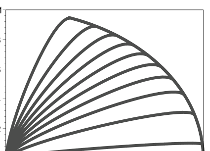
Figure 1: The phase plane for $\eta=0.9$. The point ($X=0,\ Y=0$) corresponds to the dark energy dominated epoch. It is stable and thus an attractor. The point ($X=0,\ Y=1$) corresponds to the radiation dominated epoch at which the dark energy has the equation of state $-5/3$. The point ($X=1,\ Y=0$) corresponds to the matter dominated epoch at which the dark energy has also the equation of state $-5/3$. These trajectories show that the Universe always evolves from the radiation dominated epoch to the dark energy dominated epoch.

In Fig. 1, we plot the phase portraits for $\eta=0.9$ with vast initial conditions. For $\eta=0.9$, we have three critical points, namely, point (0, 0), (0, 1) and (1, 0). The point (0, 0) corresponds to the dark energy dominated epoch and the circled arc ($X^{2}+Y^{2}=1$) corresponds to the matter and radiation co-dominated epoch. The point (0, 0) is stable and thus an attractor. The point (1, 0) is the matter dominated epoch and it is a saddle point. The point (0, 1) is the radiation dominated epoch and it is unstable. Since this point is unstable, we conclude that the Universe always evolves from the radiation dominated epoch to the dark energy dominated epoch shown by the portrait.

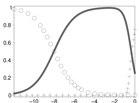
Figure 2: The evolution of density fractions for radiation ($Y^{2}$) (circled line), matter ($X^{2}$) (solid line) and dark energy ($\Omega_{\phi}$) (crossed line), for the value $\eta=0.9$.

In Fig. 2, we plot the evolution of density fractions for radiation, matter and holographic dark energy, for the parameter $\eta=0.9$. The solid line represents the density fraction of the matter. The circled line and crossed line represent the density fraction for the radiation and dark energy, respectively.

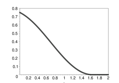
Figure 3: The evolution of the dimensionless energy density $\eta/u^{2}$ of holographic dark energy with redshift. The energy density of dark energy approaches zero at redshifts greater than $1.6$.

In Fig. 3, we plot the evolution of the dimensionless energy density $\eta/u^{2}$ of holographic dark energy with redshift. Since the density of dark energy approaching zero at redshifts greater than $1.6$, this shows that dark energy should not play a key role in the history of structure formation. Also, the coincidence problem coin:2000 is greatly relaxed because the scalar field emerges very recently.

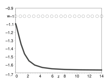
Figure 4: The equation of the state of the dark energy. Since the equation of state is always smaller than $-1$, it belongs to the phantom dark energy models. The present-day equation of state is $-1.1$ which is consistent with observations.

In Fig. 4, we plot the equation of state $w$ for dark energy. Since the equation of state is always smaller than $-1$, the dark energy belongs to the phantom dark energy models. For the present universe, the equation of state is $-1.1$. This is consistent with observations komatsu:2009 .

In Fig. 5, we plot the deceleration parameter $q$ for the Universe. Fig. 5 tells us the Universe speeds up around redshift $z_{T}=0.86$ which is not inconsistent with astronomical observations.

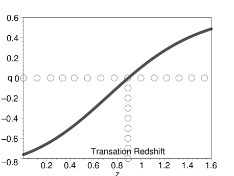
Figure 5: The deceleration parameter $q$ with the redshift. The Universe speeds up around redshift $z_{T}=0.86$ which is not inconsistent with astronomical observations.

V conclusion and discussion

Scalar fields may originate from the extra space dimensions, for example, in Kaluza-Klein compactification theory as the radion csaki:2000 , in the low-energy limit of the superstring theory as the dilaton gibbons:1985 or tachyon sen:2002 . In this paper, we propose the scalar field originates from the four dimensional spacetime geometry. In order that the theory leads to the second order differential equations, one should let $\phi$ be the function of the four dimensional volume. For simplicity, we identify $\phi$ with the four dimensional volume. Motivated by Faraoni’s work faraoni:2011 , we rewrite the FRW metric in the Schwarzschild coordinate system and then calculate the four dimensional volume.

For the specific form of Lagrangian $\propto 1/\sqrt[3]{U}$, the model gives the holographic dark energy where the density of dark energy is inversely proportional to the square of the radius of null hypersurface. We note that this null hypersurface is different from the Hubble horizon, the event horizon, the particle horizon and the apparent horizon. In order to interpret the current acceleration of the Universe, this holographic dark energy belongs to the phantom dark energy.

Is this holographic dark energy consistent with the solar system tests on General Relativity? The answer is yes. The reason could be understood as follows. The gravitational field in the solar system can be very well described by the Schwarzschild solution

$$ds^{2}=-\left(1-\frac{2M}{r}\right)dt^{2}+\left(1-\frac{2M}{r}\right)^{-1}dr^{2}+r^{2}d\Omega^{2}\;,$$ (53)

where $M$ is the mass of the Sun. The four dimensional volume of the spacetime is

$$\texttt{V}=\int d^{4}x\sqrt{-g}=\int_{0}^{L_{\infty}}{4}\pi r^{2}dr\int_{0}^{t}dt=\frac{32}{3}\pi L_{\infty}^{3}t\;.$$ (54)

Here $L_{\infty}$ stands for the maximum scale in the Universe which can be taken as the Universe scale $L_{\infty}=\bar{r}_{N}$. Then the Lagrangian (Eq. (39)) becomes

$$\mathscr{L}\propto\sqrt{-g}\cdot\frac{1}{\bar{r}_{N}^{2}}\;.$$ (55)

We know from the dimensional analysis that the Ricci scalar $R\simeq{L^{-2}}$ with $L$ some scale within the solar system. It is apparent that

$$\frac{1}{\bar{r}_{N}^{2}}\ll\frac{1}{L^{2}}\;,$$ (56)

in the solar system. So the Lagrangian (Eq. (55)) can be safely neglected compared to the Einstein-Hilbert action. In other words, the gravitational field in the solar system can be very well described by the Schwarzschild solution.

- (1) C. Brans and R. H. Dicke, Phys. Rev. D 124, 925 (1961)
- (2) C. Csaki, M. Graesser, L. Randall, J. Terning, Phys. Rev. D 62, 045015 (2000)
- (3) P. W. Higgs, Phys. Lett. B 12, 132 (1964)
- (4) G. W. Gibbons, K. Maeda, Nucl. Phys. B 298, 741 (1988)
- (5) Sen, A., JHEP. 0204, 048 (2002)
- (6) A. H. Guth, Phys. Rev. D 23, 347 (1981)
- (7) B. Ratra and J. Peebles, Phys. Rev. D 37, 321 (1988)
- (8) R. R. Caldwell, R. Dave and P. J. Steinhardt, Phys. Rev. Lett. 80, 1582 (1998)
- (9) Zlatev, L. Wang, P. J. Steinhardt, Phys. Rev. Lett. 82, 896 (1999)
- (10) R. R. Caldwell, Phys. Lett. B 545, 23 (2002)
- (11) C. Armendariz-Picon, V. F. Mukhanov and P. J. Steinhardt, Phys. Rev. Lett. 85, 4438 (2000) [astro-ph/0004134]; C. Armendariz-Picon, V. F. Mukhanov and P. J. Steinhardt, Phys. Rev. D 63, 103510 (2001) [astro-ph/0006373]; R. J. Scherrer, Phys. Rev. Lett. 93, 011301 (2004)
- (12) M. Li, Phys.Lett. B603 (2004) 1.
- (13) A. Cohen, D. Kaplan and A. Nelson, Phys. Rev. Lett. 82 (1999) 4971; P. Horava and D. Minic, hep-th/hep-th/0001145, Phys.Rev.Lett. 85 (2000) 1610; S. Thomas, Phys. Rev. Lett. 89 (2002) 081301; S. Nojiri and S. D. Odintsov, Gen. Rel. Grav. 38, 1285 (2006); X. Zhang, F. Q. Wu, Phys. Rev. D 72 (2005) 043524; Z. Chang, F.Q. Wu, X. Zhang, Phys.Lett.B 633 (2006) 14; J. Zhang, X. Zhang, H. Liu Phys.Lett.B651 (2007) 84; Y. Ma, X. Zhang, Phys.Lett.B 661 (2008) 239; L. Xu, W. Li J. Lu arXiv: 0810.4730; C.J. Feng, Phys. Lett. B 670, 231 (2008); L.N. Granda and A. Oliveros, Phys. Lett. B 669, 275 (2008); Q.G. Huang and M. Li, JCAP 0408, 013 (2004); Y.G. Gong, B. Wang and Y.Z. Zhang Phys. Rev. D 72, 043510 (2005); B. Wang, Y.G. Gong and E. Abdalla, Phys. Lett. B 624, 141 (2005); B. Chen, M. Li and Y. Wang, Nucl. Phys. B 774, 256 (2007); I.P. Neupane, Phys. Rev. D 76, 123006 (2007); J.P. Wu, D.Z. Ma and Y. Ling, Phys. Lett. B 663, 152 (2008); H. Wei and R.G. Cai, Eur. Phys. J. C 59, 99 (2009); Z. Yi and T. Zhang, Mod. Phys. Lett. A. 22, 41 (2007); E. N. Saridakis, Phys. Lett. B 660, 138 (2008); E. N. Saridakis, JCAP. 0804, 020 (2008); Phys. Lett. B 661, 335 (2008)
- (14) R. G. Cai, Phys. Lett. B 657, 228 (2007); Z. Zhai, T. Zhang and W. Liu, JCAP. 8, 019 (2011); T. Zhang, C. Ma and T. Lan, Advances in Astronomy, 2010, 184284, 2010
- (15) H. Wei and R. G. Cai, Phys. Lett. B 660, 113 (2008); O. A. Lemets, D. A. Yerokhin and L.G. Zazunov JCAP. 01, 007 (2011)
- (16) C. Gao, F. Wu, X. Chen and Y. Shen, Phys. Rev. D 79, 043511 (2009); R. Cai, B. Hu and Y. Zhang, Commun. Theor. Phys. 51, 954 (2009)
- (17) R. Yang, Z. Zhu and F. Wu, Int. J. Mod. Phy. A 26, 317 (2011)
- (18) W. Fischler and L. Susskind, hep-th/9806039; R. Bousso, JHEP 9907 (1999) 004.
- (19) V. Faroni, Phys. Rev. D 84, 024003 (2011)
- (20) W. Rindler, Mon. Not. R. Astr. Soc. 116 (1956) 663. Reprinted in Gen. Rel. Gravit. 34 (2002) 133
- (21) S.A. Hayward, Phys. Rev. D 49, 6467 (1994); Y. Gong and A. Wang, Phys. Rev. Lett. 99, 211301 (2007); M. Akbar and R.G. Cai, Phys. Rev. D 75, 084003 (2007); R.G. Cai and L.M. Cao, Phys. Rev. D 75, 064008 (2007); R.G. Cai and L.M. Cao, Nucl. Phys. B 785, 135 (2007); M. Akbar and R.G. Cai, Phys. Lett. B 648, 243 (2007); A. Sheykhi, B. Wang and R.G. Cai, Phys. Rev. D 76, 023515 (2007); A. Sheykhi, B. Wang and R.G. Cai, Nucl. Phys. B 779, 1 (2007).
- (22) E. J. Copeland, A. R. Liddle, and D. Wands, Phys. Rev. D57, 4686 (1998), arXiv:gr-qc/9711068.
- (23) E. Komatsu et al, Astrophys. J. Suppl. 180, 330 (2009).
- (24) S. Weinberg, astro-ph/0005265.