Controlling overestimation of error covariance in ensemble Kalman filters with sparse observations: A variance limiting Kalman filter

Abstract

We consider the problem of an ensemble Kalman filter when only partial observations are available. In particular we consider the situation where the observational space consists of variables which are directly observable with known observational error, and of variables of which only their climatic variance and mean are given. To limit the variance of the latter poorly resolved variables we derive a variance limiting Kalman filter (VLKF) in a variational setting. We analyze the variance limiting Kalman filter for a simple linear toy model and determine its range of optimal performance. We explore the variance limiting Kalman filter in an ensemble transform setting for the Lorenz-96 system, and show that incorporating the information of the variance of some un-observable variables can improve the skill and also increase the stability of the data assimilation procedure.

1 Introduction

In data assimilation one seeks to find the best estimation of the state of a dynamical system given a forecast model with a possible model error and noisy observations at discrete observation intervals (Kalnay, 2002). This process is complicated on the one hand by the often chaotic nature of the underlying nonlinear dynamics leading to an increase of the variance of the forecast, and on the other hand by the fact that one often has only partial information of the observables. In this paper we address the latter issue. We consider situations whereby noisy observations are available for some variables but not for other unresolved variables. However, for the latter we assume that some prior knowledge about their statistical climatic behaviour such as their variance and their mean is available.

A particularly attractive framework for data assimilation are ensemble Kalman filters (see for example Evensen (2006)). These straightforwardly implemented filters distinguish themselves from other Kalman filters in that the spatially and temporally varying background error covariance is estimated from an ensemble of nonlinear forecasts. Despite the ease of implementation and the flow-dependent estimation of the error covariance ensemble Kalman filters are subject to several errors and specific difficulties (see Ehrendorfer (2007) for a recent review). Besides the problems of estimating model error which is inherent to all filters, and inconsistencies between the filter assumptions and reality such as non-Gaussianity which render all Kalman filters suboptimal, ensemble based Kalman filters have the specific problem of sampling errors due to an insufficient size of the ensemble. These errors usually underestimate the error covariances which may ultimately lead to filter divergence when the filter trusts its own forecast and ignores the information given by the observations.

To counteract the associated small spread of the ensemble several techniques have been developed. To deal with errors in ensemble filters due to sampling errors we mention two of the main algorithms, covariance inflation and localisation. To avoid filter divergence due to an underestimation of error covariances the concept of covariance inflation was introduced whereby the prior forecast error covariance is increased by an inflation factor (Anderson and Anderson, 1999). This is usually done in a global fashion and involves careful and expensive tuning of the inflation factor; however recently methods have been devised to adaptively estimate the inflation factor from the innovation statistics (Anderson, 2007, 2009; Li et al., 2009). Too small ensemble sizes also lead to spurious correlations associated with remote observations. To address this issue the concept of localization has been introduced (Houtekamer and Mitchell, 1998, 2001; Hamill et al., 2001; Ott et al., 2004; Szunyogh et al., 2005) whereby only spatially close observations are used for the innovations.

To take into account the uncertainty in the model representation we mention here isotropic model error parametrization (Mitchell and Houtekamer, 2000; Houtekamer et al., 2005), stochastic parametrizations (Buizza et al., 1999) and kinetic energy backscatter (Shutts, 2005). A recent comparison between those methods is given in Houtekamer et al. (2009); Charron et al. (2010), see also Hamill and Whitaker (2005). The problem of non-Gaussianity is for example discussed in Pires et al. (2010); Bocquet et al. (2010).

Whereas the underestimation of error covariances has received much attention, relatively little is done for a possible overestimation of error covariances. Overestimation of covariance is a finite ensemble size effect which typically occurs in sparse observation networks (see for example Liu et al. (2008); Whitaker et al. (2009)). Uncontrolled growth of error covariances which is not tempered by available observations may progressively spoil the overall analysis. This effect is even exacerbated when inflation is used; in regions where no observations influence the analysis, inflation can lead to unrealistically large ensemble variances progressively degrading the overall analysis (see for example Whitaker et al. (2004)). This is particularly problematic when inappropriate uniform inflation is used. Moreover, it is well known that covariance localization can be a significant source of imblance in the analyzed fields (see for example Houtekamer and Mitchell (2005); Kepert (2009); Houtekamer et al. (2009)). Localization artificially generates unwanted gravity wave activity which in poorly resolved spatial regions may lead to an unrealistic overestimation of error covariances. Being able to control this should help filter performances considerably.

When assimilating current weather data in numerical schemes for the troposphere, the main problem is underestimation of error covariances rather than overestimation. This is due to the availability of radiosonde data which assures wide observational coverage. However, in the pre-radiosonde era there were severe data voids, particularly in the southern hemisphere and in vertical resolution since most observations were done on the surface level in the northern hemisphere. There is an increased interest in so called climate reanalysis (see for example (Bengtsson et al., 2007; Whitaker et al., 2004)), which has the challenge to deal with large unobserved regions. Historical atmospheric observations are reanalyzed by a fixed forecast scheme to provide a global homogeneous dataset covering troposphere and stratosphere for very long periods. A remarkable effort is the international Twentieth Century Reanalysis Project (20CR) (Compo et al., 2011), which produced a global estimate of the atmosphere for the entire 20th century (1871 to the present) using only synoptic surface pressure reports and monthly sea-surface temperature and sea-ice distributions. Such a dataset could help to analyze climate variations in the twentieth century or the multidecadal variations in the behaviour of the El-Niño-Southern Oscillation. An obstacle for reanalysis is the overestimation of error covariances if one chooses to employ ensemble filters (Whitaker et al. (2004) where multiplicative covariance inflation is employed).

Overestimation of error covariances occurs also in modern numerical weather forecast schemes for which the upper lid of the vertical domain is constantly pushed towards higher and higher levels to incorporate the mesosphere, with the aim to better resolve processes in the polar stratosphere (see for example Polavarapu et al. (2005); Sankey et al. (2007); Eckermann et al. (2009)). The energy spectrum in the mesosphere is, contrary to the troposphere, dominated by gravity waves. The high variability associated with these waves causes very large error covariances in the mesosphere which can be $2$ orders of magnitude larger than at lower levels (Polavarapu et al., 2005), rendering the filter very sensitive to small uncertainties in the forecast covariances. Being able to control the variances of mesospheric gravity waves is therefore a big challenge.

The question we address in this work is how can the statistical information available for some data which are otherwise not observable, be effectively incorporated in data assimilation to control the potentially high error covariances associated with the data void. We will develop a framework to modify the familiar Kalman filter (see for example (Evensen, 2006; Simon, 2006)) for partial observations with only limited information on the mean and variance, with the effect that the error covariance of the unresolved variables cannot exceed their climatic variance and their mean is controlled by driving it towards the climatological value.

The paper is organized as follows. In Section 2 we will introduce the dynamical setting and briefly describe the ensemble transform Kalman filter (ETKF), a special form of an ensemble square root filter. In Section 3 we will derive the variance limiting Kalman filter (VLKF) in a variational setting. In Section 4 we illustrate the VLKF with a simple linear toy model for which the filter can be analyzed analytically. We will extract the parameter regimes where we expect VLKF to yield optimal performance. In Section 5 we apply the VLKF to the $40$-dimensional Lorenz-96 system (Lorenz, 1996) and present numerical results illustrating the advantage of such a variance limiting filter. We conclude the paper with a discussion in section 6.

2 Setting

Assume an $N$-dimensional dynamical system whose dynamics is given by

$$\dot{\bf z}=f({\bf z})\;,$$ (1)

with the state variable ${\bf z}\in\mathbb{R}^{N}$. We assume that the state space is decomposable according to ${\bf z}=({\bf x},{\bf y})$ with ${\bf x}\in\mathbb{R}^{n}$ and ${\bf y}\in\mathbb{R}^{m}$ and $n+m=N$. Here ${\bf x}$ shall denote those variables for which direct observations are available, and ${\bf y}$ shall denote those variables for which only some integrated or statistical information is available. We will coin the former observables and the latter pseudo-observables. We do not incorporate model error here and assume that (1) describes the truth. We apply the notation of Ide et al. (1997) unless stated explicitly otherwise.

Let us introduce an observation operator ${\bf{H}}:\mathbb{R}^{N}\to\mathbb{R}^{n}$ which maps from the whole space into observation space spanned by the designated variables ${\bf{x}}$. We assume that observations of the designated variables ${\bf{x}}$ are given at equally spaced discrete observation times $t_{i}$ with the observation interval $\Delta t_{\rm{obs}}$. Since it is assumed that there is no model error, the observations ${{\bf{{\bf{y}}_{\rm{o}}}}}\in\mathbb{R}^{n}$ at discrete times $t_{i}=i\Delta t_{\rm{obs}}$ are given by

$${{\bf{{\bf{y}}_{\rm{o}}}}}(t_{i})={\bf{H}}{\bf{z}}(t_{i})+{{\bf{r}}_{\rm{o}}}\,,$$

with independent and identically distributed (i.i.d.) observational Gaussian noise ${\bf{r}}_{\rm{o}}\in\mathbb{R}^{n}$. The observational noise is assumed to be independent of the system state, and to have zero mean and constant covariance ${\bf{R}}_{\rm{o}}\in\mathbb{R}^{n\times n}$.

We further introduce an operator ${\bf{h}}:\mathbb{R}^{N}\to\mathbb{R}^{m}$ which maps from the whole space into the space of the pseudo-observables spanned by ${\bf{y}}$. We assume that the pseudo-observables have variance ${\bf{A}}_{\rm{clim}}\in\mathbb{R}^{m\times m}$ and constant mean ${\bf{a}}_{\rm{clim}}\in\mathbb{R}^{m}$. This is the only information available for the pseudo-observables, and may be estimated, for example, from climatic measurements. The error covariance of those pseudo-observations is denoted by ${\bf{R}}_{\rm{w}}\in\mathbb{R}^{m\times m}$.

The model forecast state ${\bf{z}}_{f}$ at each observation interval is obtained by integrating the state variable with the full nonlinear dynamics (1) for the time interval $\Delta t_{\rm{obs}}$. The background (or forecast) involves an error with covariance ${\bf{P}}_{f}\in\mathbb{R}^{N\times N}$.

Data assimilation aims to find the best estimation of the current state given the forecast ${\bf{z}}_{f}$ with variance ${\bf{P}}_{f}$ and observations ${\bf{{\bf{y}}_{\rm{o}}}}$ of the designated variables with error covariance ${\bf{R}}_{\rm{o}}$. Pseudo-observations can be included following the standard Bayesian approach once their mean ${\bf{a}}_{\rm{clim}}$ and error covariance ${\bf{R}}_{\rm{w}}$ are known. However, the error covariance ${\bf{R}}_{\rm{w}}$ of a pseudo-observation is in general not equal to ${\bf{A}}_{\rm{clim}}$. In Section 3, we will show how to derive the error covariance ${\bf{R}}_{\rm{w}}$ in order to ensure that the forecast does not exceed the prescribed variance ${\bf{A}}_{\rm{clim}}$. We do so in the framework of Kalman filters and shall now briefly summarize the basic ideas to construct such a filter for the case of an ensemble square root filter (Tippett et al., 2003), the ensemble transform filter (Wang et al., 2004).

2.1 Ensemble Kalman filter

In an ensemble Kalman filter (EnKF) (Evensen, 2006) an ensemble with $k$ members ${\bf{z}}_{k}$

$${\bf{Z}}=\left[{\bf{z}}_{1},{\bf{z}}_{2},\dots,{\bf{z}}_{k}\right]\in\mathbb{R}^{N\times k}$$

is propagated by the full nonlinear dynamics (1), which is written as

$${\dot{{\bf{Z}}}}={\bf{f}}({\bf{Z}})\;,\qquad{\bf{f}}({\bf{Z}})=\left[f({\bf{z}}_{1}),f({\bf{z}}_{2}),\dots,f({\bf{z}}_{k})\right]\in\mathbb{R}^{N\times k}\;.$$ (2)

The ensemble is split into its mean

$${\bar{{\bf{z}}}}=\frac{1}{k}\sum_{i=1}^{k}{\bf{z}}_{i}={\bf{Z}}{\bf{w}}\qquad{\rm{with}}\qquad{\bf{w}}=\frac{1}{k}{\bf{e}}\in\mathbb{R}^{k}\;,$$

where ${\bf{e}}=\left[1,\dots,1\right]^{T}\in\mathbb{R}^{k}$, and its ensemble deviation matrix

$${\bf{Z}}^{\prime}={\bf{Z}}-{\bar{{\bf{z}}}}{\bf{e}}^{T}={\bf{Z}}{\bf{T}}\;,$$

with the constant projection matrix

$${\bf{T}}={\bf{I}}-{\bf{w}}{\bf{e}}^{T}\in\mathbb{R}^{k\times k}\;.$$

The ensemble deviation matrix ${\bf{Z}}^{\prime}$ can be used to approximate the ensemble forecast covariance matrix via

$${\bf{P}}_{f}(t)=\frac{1}{k-1}{\bf{Z}}^{\prime}(t)\left[{\bf{Z}}^{\prime}(t)\right]^{T}\in\mathbb{R}^{N\times N}\;.$$

Given the forecast ensemble ${\bf{Z}}_{f}={\bf{Z}}(t_{i}-\epsilon)$ and the associated forecast error covariance matrix (or the prior) ${\bf{P}}_{f}(t_{i}-\epsilon)$, the actual Kalman analysis (Kalnay, 2002; Evensen, 2006; Simon, 2006) updates a forecast into a so-called analysis (or the posterior). Variables at times $t=t_{i}-\epsilon$ are evaluated before taking the observations (and/or pseudo-observations) into account in the analysis step, and variables at times $t=t_{i}+\epsilon$ are evaluated after the analysis step when the observations (and/or pseudo-observations) have been taken into account. In the first step of the analysis the forecast mean,

$${\bar{{\bf{z}}}}_{f}={\bf{Z}}_{f}{\bf{w}}\;,$$

is updated to the analysis mean

$${\bar{{\bf{z}}}}_{a}={\bar{{\bf{z}}}}_{f}-{\bf{K}}_{\rm{o}}\left[{\bf{H}}{\bar{{\bf{z}}}}_{f}-{{\bf{{\bf{y}}_{\rm{o}}}}}\right]-{\bf{K}}_{\rm{w}}\left[{\bf{h}}{\bar{{\bf{z}}}}_{f}-{\bf{a}}_{\rm{clim}}\right]\;,$$ (3)

where the Kalman gain matrices are defined as

$${\bf{K}}_{\rm{o}} = {\bf{P}}_{a}{\bf{H}}^{T}{\bf{R}}^{-1}_{\rm{o}}$$

$${\bf{K}}_{\rm{w}} = {\bf{P}}_{a}{\bf{h}}^{T}{\bf{R}}^{-1}_{\rm{w}}\;.$$ (4)

The analysis covariance ${\bf{P}}_{a}$ is given by the addition rule for variances, typical in linear Kalman filtering (Kalnay, 2002),

$${\bf{P}}_{a}=\left({\bf{P}}_{f}^{-1}+{\bf{H}}^{T}{\bf{R}}^{-1}_{\rm{o}}{\bf{H}}+{\bf{h}}^{T}{\bf{R}}^{-1}_{\rm{w}}{\bf{h}}\right)^{-1}\,.$$ (5)

To calculate an ensemble ${\bf{Z}}_{a}$ which is consistent with the error covariance after the observation ${\bf{P}}_{a}$, and which therefore needs to satisfy

$${\bf{P}}_{a}=\frac{1}{k-1}{\bf{Z}}_{a}{\bf{T}}\left[{\bf{Z}}_{a}\right]^{T}\;,$$

we use the method of ensemble square root filters (Simon, 2006). In particular we use the method proposed in (Tippett et al., 2003; Wang et al., 2004), the so called ensemble transform Kalman filter (ETKF), which seeks a transformation ${\bf{S}}\in\mathbb{R}^{k\times k}$ such that

$${\bf{Z}}_{a}^{\prime}={\bf{Z}}_{f}^{\prime}{\bf{S}}\;.$$ (6)

Alternatively one could have chosen the ensemble adjustment filter (Anderson, 2001) in which the ensemble deviation matrix ${\bf{Z}}_{f}^{\prime}$ is pre-multiplied with an appropriately determined matrix ${\bf{A}}\in\mathbb{R}^{N\times N}$. However, since we are mainly interested in the case $k\ll N$ we shall use the ETKF. Note that the matrix ${\bf{S}}$ is not uniquely determined for $k<N$. The transformation matrix ${\bf{S}}$ can be obtained either by using continuous Kalman filters (Bergemann et al., 2009) or directly (Wang et al., 2004) by

$${\bf{S}}={\bar{{\bf{C}}}}\left({\bf{I}}_{k}+{\bar{{\bf{\Gamma}}}}\right)^{-\frac{1}{2}}{\bar{{\bf{C}}}}^{T}\;.$$

Here ${\bf{C}}{\bf{\Gamma}}{\bf{C}}^{T}$ is the singular value decomposition of

$${\bf{U}}=\frac{1}{k-1}{\bf{T}}^{T}{\bf{Z}}_{f}^{T}\left({\bf{H}}^{T}{\bf{R}}^{-1}_{\rm{o}}{\bf{H}}+{\bf{h}}^{T}{\bf{R}}^{-1}_{\rm{w}}{\bf{h}}\right){\bf{Z}}_{f}{\bf{T}}\;.$$

The matrix ${\bar{{\bf{C}}}}\in\mathbb{R}^{k\times(k-1)}$ is obtained by erasing the last zero column from ${\bf{C}}\in\mathbb{R}^{k\times k}$, and ${\bar{{\bf{\Gamma}}}}\in\mathbb{R}^{(k-1)\times(k-1)}$ is the upper left $(k-1)\times(k-1)$ block of the diagonal matrix ${\bf{\Gamma}}\in\mathbb{R}^{k\times k}$. The deletion of the $0$ eigenvalue and the associated columns in ${\bf{C}}$ assure that ${\bf{Z}}_{a}^{\prime}={\bf{Z}}_{a}^{\prime}{\bf{S}}$ and therefore that the analysis mean is given by ${\bar{{\bf{z}}}}_{a}$. Note that ${\bf{S}}$ is symmetric and ${\bf{S}}{\bf{T}}={\bf{T}}{\bf{S}}$ which assures that ${\bf{Z}}_{a}^{\prime}={\bf{Z}}_{a}^{\prime}{\bf{S}}$ implying that the mean is preserved under the transformation. This is not necessarily true for general ensemble transform methods of the form (6).

A new forecast ${\bf{Z}}(t_{i+1}-\epsilon)$ is then obtained by propagating ${\bf{Z}}_{a}$ with the full nonlinear dynamics (2) to the next time of observation. The numerical results presented later in Sections 4 and 5 are obtained with this method.

In the next Section we will determine how the error covariance ${\bf{R}}_{\rm{w}}$ used in the Kalman filter is linked to the variance ${\bf{A}}_{\rm{clim}}$ of the pseudo-variables.

3 Derivation of the variance limiting Kalman filter

One may naively believe that the error covariance of the pseudo-observable ${\bf{R}}_{\rm{w}}$ is determined by the target variance of the pseudo-observables ${\bf{A}}_{\rm{clim}}$ simply by setting ${\bf{R}}_{\rm{w}}={\bf{A}}_{\rm{clim}}$. In the following we will see that this is not true, and that the expression for ${\bf{R}}_{\rm{w}}$ which ensures that the variance of the pseudo-observables in the analysis is limited from above by ${\bf{A}}_{\rm{clim}}$ involves all error covariances.

We formulate the Kalman filter as a minimization problem of a cost function (e.g. Kalnay (2002)). The cost function for one analysis step as described in Section 2.1 with a given background ${\bf{z}}_{f}$ and associated error covariance ${\bf{P}}_{f}$ is typically written as

$$J({{\bf{z}}}) = \frac{1}{2}({{\bf{z}}}-{{\bf{z}}}_{f})^{T}{\bf{P}}_{f}^{-1}({\bf{z}}-{\bf{z}}_{f})+\frac{1}{2}({\bf{{\bf{y}}_{\rm{o}}}}-{\bf{H}}{\bf{z}})^{T}{\bf{R}}^{-1}_{\rm{o}}({\bf{{\bf{y}}_{\rm{o}}}}-{\bf{H}}{\bf{z}})$$ (7)

$$+\;\frac{1}{2}({\bf{a}}_{\rm{clim}}-{\bf{h}}{\bf{z}})^{T}{\bf{R}}^{-1}_{\rm{w}}({\bf{a}}_{\rm{clim}}-{\bf{h}}{\bf{z}})\;,$$

where ${\bf{z}}$ is the state variable at one observation time $t_{i}=i\Delta t_{\rm{obs}}$. Note that the part involving the pseudo-observables corresponds to the notion of weak constraints in variational data assimilation (Sasaki, 1970; Zupanski, 1997; Neef et al., 2006).

The analysis step of the data assimilation procedure consists of finding the critical point of this cost function. The thereby obtained analysis ${{\bf{z}}={\bar{\bf{z}}}_{a}}$ and the associated variance ${\bf{P}}_{a}$ are then subsequently propagated to the next observation time $t_{i+1}$ to yield ${{\bf{z}}}_{f}$ and ${\bf{P}}_{f}$ at the next time step, at which a new analysis step can be performed. The equation for the critical point with $\nabla_{{{\bf{z}}}}J({{\bf{z}}})=0$ is readily evaluated to be

$$\left({\bf{P}}_{f}^{-1}+{{\bf{H}}}^{T}{\bf{R}}^{-1}_{\rm{o}}{\bf{H}}+{{\bf{h}}}^{T}{\bf{R}}^{-1}_{\rm{w}}{\bf{h}}\right){\bf{z}}_{a}={\bf{P}}_{f}^{-1}{\bf{z}}_{f}+{{\bf{H}}}^{T}{\bf{R}}^{-1}_{\rm{o}}{{\bf{{\bf{y}}_{\rm{o}}}}}+{\bf{h}}^{T}{\bf{R}}^{-1}_{\rm{w}}{\bf{a}}_{\rm{clim}}\;,$$ (8)

and yields (3) for the analysis mean ${\bar{\bf{z}}}_{a}$, and (5) for the analysis covariance ${\bf{P}}_{a}$ with Kalman gain matrices given by (4).

To control the variance of the unresolved pseudo-observables ${\bf{a}}_{\rm{clim}}={\bf{h}}{\bf{z}}$ we set

$${\bf{h}}{\bf{P}}_{a}{\bf{h}}^{T}={\bf{A}}_{\rm{clim}}\;.$$ (9)

Introducing

$${\bm{{\mathcal{P}}}}^{-1}={\bf{P}}_{f}^{-1}+{\bf{H}}^{T}{\bf{R}}^{-1}_{\rm{o}}{\bf{H}}\;,$$ (10)

and upon applying the Sherman-Morrison-Woodbury formula (see for example Golub and Loan (1996)) to $({\bm{{\mathcal{P}}}}^{-1}+{\bf{h}}^{T}{\bf{R}}^{-1}_{\rm{w}}{\bf{h}})^{-1}$, equation (9) yields the desired equation for ${\bf{R}}_{\rm{w}}$

$${\bf{R}}^{-1}_{\rm{w}}={\bf{A}}^{-1}_{\rm{clim}}-\left({\bf{h}}{\bm{{\mathcal{P}}}}{\bf{h}}^{T}\right)^{-1}\;,$$ (11)

which is yet again a reciprocal addition formula for variances. Note that the naive expectation that ${\bf{R}}_{\rm{w}}={\bf{A}}_{\rm{clim}}$ is true only for ${\bf{P}}_{f}\to\infty$, but is not generally true. For sufficiently small background error covariance ${\bf{P}}_{f}$, the error covariance ${\bf{R}}_{\rm{w}}$ as defined in (11) is not positive semi-definite. In this case the information given by the pseudo-observables has to be discarded. In the language of variational data assimilation the criterion of positive definiteness of ${\bf{R}}^{-1}_{\rm{w}}$ determines whether the weak constraint is switched on or off. To determine those eigendirections for which the statistical information available can be incorporated, we diagonalize ${\bf{R}}^{-1}_{\rm{w}}={\bf{V}}{\bf{D}}{\bf{V}}^{T}$ and define ${\bar{{\bf{D}}}}$ with ${\bar{{\bf{D}}}}_{ii}={\bf{D}}_{ii}$ for ${\bf{D}}_{ii}\geq 0$ and ${\bar{{\bf{D}}}}_{ii}=0$ for ${\bf{D}}_{ii}<0$. The modified ${\bf{R}}^{-1}_{\rm{w}}={\bf{V}}{\bar{{\bf{D}}}}{\bf{V}}^{T}$ then uses information of the pseudo-observables only in those directions which potentially allow for improvement of the analysis. Noting that ${\bm{{\mathcal{P}}}}$ denotes the analysis covariance of an ETKF (with ${\bf{R}}_{\rm{w}}=0$), we see that equation (11) states that the variance constraint switches on for those eigendirections whose corresponding singular eigenvalues of ${\bf{h}}{\bm{{\mathcal{P}}}}{\bf{h}}^{T}$ are larger than those of ${\bf{A}}_{\rm{clim}}$. Hence the proposed VLKF as defined here incorporates the climatic information of the unresolved variables in order to restrict the posterior error covariance of those pseudo-observables to lie below their climatic variance and to drive the mean towards their climatological mean.

4 Analytical linear toy model

In this Section we study the VLKF for the following coupled linear skew product system for two oscillators ${\bf{x}}\in\mathbb{R}^{2}$, ${\bf{y}}\in\mathbb{R}^{2}$

$${d{\bf{x}}} = {\bm{A}}{\bf{x}}\,dt-{\bm{\Gamma}_{\bm{x}}}\,{\bf{x}}\,dt+{\bm{\sigma}_{\bm{x}}}d{\bm{W}}_{t}+{\mathbf{\Lambda}}{\bf{y}}\,dt$$

$${d{\bf{y}}} = {\bm{B}}{\bf{y}}\,dt-{\bm{\Gamma}_{\bm{y}}}\,{\bf{y}}\,dt+{\bm{\sigma}_{\bm{y}}}d{\bm{B}}_{t}\;,$$

where $\bm{A}$, $\bm{B}$ and $\bm{\Lambda}$ are all skew-symmetric, $\bm{\sigma}_{\bm{x,y}}$ and $\bm{\Gamma}_{\bm{x,y}}$ are all symmetric, and $d{\bm{W}}_{t}$ and $d{\bm{B}}_{t}$ are independent two-dimensional Brownian processes. We assume here for simplicity that

$$\bm{\Gamma}_{\bm{x}}=\gamma_{x}{\bf{I}}\,,\qquad\bm{\Gamma}_{\bm{y}}=\gamma_{y}{\bf{I}}\,,\qquad\bm{\sigma}_{\bm{x}}=\sigma_{x}{\bf{I}}\,,\qquad\bm{\sigma}_{\bm{y}}=\sigma_{y}{\bf{I}}\,,\qquad{\bf{R}}_{\rm{o}}=R_{\rm obs}{\bf{I}}\;,$$

with the identity matrix ${\bf{I}}$, and

$$\bm{A}=\omega_{x}\bm{J}\,,\qquad\bm{B}=\omega_{y}\bm{J}\,,\qquad\bm{\Lambda}=\lambda\bm{J}\;,$$

with the skew-symmetric matrix

$$\bm{J}=\left(\begin{array}[]{cc}0&-1\\ 1&\;\,\,\,0\end{array}\right)\;.$$

Note that our particular choice for the matrices implies ${\bf{R}}_{\rm{w}}=R_{w}{\bf{I}}$.

The system models two noisy coupled oscillators, ${\bf{x}}$ and ${\bf{y}}$. We assume that we have access to observations of the variable ${\bf{x}}$ at discrete observation times $t_{i}=i\Delta t_{\rm{obs}}$, but have only statistical information about the variable ${\bf{y}}$. We assume knowledge of the climatic mean $\bm{\mu}_{\rm clim}$ and the climatic covariance $\bm{\sigma}_{\rm clim}^{2}$ of the unobserved variable ${\bf{y}}$. The noise is of Ornstein-Uhlenbeck type (Gardiner, 2003), and may represent either model error or parametrize highly chaotic nonlinear dynamics. Without loss of generality, the coupling is chosen such that the ${\bf{y}}$-dynamics drives the ${\bf{x}}$-dynamics but not vice versa. The form of the coupling is not essential for our argument, and it may be oscillatory or damping with $\bm{\Lambda}=\lambda{\bf{I}}$. We write this system in the more compact form for ${\bf{z}}=({\bf{x}},{\bf{y}})\in\mathbb{R}^{4}$

$${d{\bf{z}}} = {\bm{M}}{\bf{z}}\,dt-{\bm{\Gamma}}{\bf{z}}\,dt+{\bm{\sigma}}\,d{\bm{W}}_{t}+{\bm{C}}{\bf{z}}\,dt$$ (12)

with

$$\bm{M}=\left(\begin{array}[]{cc}\bm{A}&\bm{0}\\ \bm{0}&\bm{B}\end{array}\right)\qquad\bm{\Gamma}=\left(\begin{array}[]{cc}\bm{\Gamma}_{\bm{x}}&\bm{0}\\ \bm{0}&\bm{\Gamma}_{\bm{y}}\end{array}\right)$$

$${\bm{\sigma}}=\left(\begin{array}[]{cc}\bm{\sigma}_{x}&\bm{0}\\ \bm{0}&\bm{\sigma}_{y}\end{array}\right)\qquad{\bm{C}}=\left(\begin{array}[]{cc}\bm{0}&\bm{\Lambda}\\ \bm{0}&\bm{0}\end{array}\right)\;.$$

The solution of (12) can be obtained using Itô’s formula and, introducing the propagator ${\bm{L}}(t)=\exp\left((\bm{M}-\bm{\Gamma}+{\bm{C}})t\right)$, which commutes with $\bm{\sigma}$ for our choice of the matrices, is given by

$${\bf{z}}(t)={\bm{L}}(t){\bf{z}}_{0}+{\bm{\sigma}}\int_{0}^{t}{\bm{L}}(t-s)\,d{\bm{W}}_{s}\;,$$

with mean

$$\bm{\mu}(t)={\bm{L}}(t){\bf{z}}_{0}\;,$$

and covariance

$${\bm{\Sigma}}(t)={\bm{\sigma}}\left(2\bm{\Gamma}-{\bm{\mathcal{C}}}\right)^{-1}\left({\bf{I}}-\exp\left(-\left(2\bm{\Gamma}-{\bm{\mathcal{C}}}\right)t\right)\right){\bm{\sigma}}^{T}\;,$$ (13)

where

$${\bm{\mathcal{C}}}=\left(\begin{array}[]{cc}\bm{0}&\bm{\Lambda}\\ -\bm{\Lambda}&\bm{0}\end{array}\right)\;.$$

The climatic mean $\bm{\mu}_{\rm clim}\in\mathbb{R}^{4}$ and covariance matrix $\bm{\Sigma}_{\rm{clim}}\in\mathbb{R}^{4\times 4}$ are then obtained in the limit $t\to\infty$ as

$$\bm{\mu}_{\rm clim}=\lim_{t\to\infty}\bm{\mu}(t)=0\;,$$

and

$$\bm{\Sigma}_{\rm clim}=\lim_{t\to\infty}{\bm{\Sigma}}(t)={\bm{\sigma}}\left(2\bm{\Gamma}-{\bm{\mathcal{C}}}\right)^{-1}{\bm{\sigma}}^{T}\;.$$

In order for the stochastic process (12) to have a stationary density and for ${\bm{\Sigma}}(t)$ to be a positive definite covariance matrix for all $t$, the coupling has to be sufficiently small with $\lambda^{2}<4\gamma_{x}\gamma_{y}$. Note that the skew product nature of the system (12) is not special in the sense that a non-skew product structure where ${\bf{x}}$ couples back to ${\bf{y}}$ would simply lead to a renormalization of ${\bm{\mathcal{C}}}$. However, it is pertinent to mention that although in the actual dynamics of the model (12) there is no back-coupling from ${\bf{x}}$ to ${\bf{y}}$, the Kalman filter generically introduces back-coupling of all variables through the inversion of the covariance matrices (cf. (5)).

We will now investigate the variance limiting Kalman filter for this toy model. In particular we will first analyze under what conditions ${\bf{R}}_{\rm{w}}$ is positive definite and the variance constraint will be switched on, and second we will analyze when the VLKF yields a skill improvement when compared to the standard ETKF.

We start with the positive definiteness of ${\bf{R}}_{\rm{w}}$. When calculating the covariance of the forecast in an ensemble filter we need to interpret the solution of the linear toy model (12) as

$${{\bf{z}}}_{j}(t_{i+1})\,{\buildrel d\over{=}}\,{\bm{L}}(\Delta t_{\rm{obs}}){{\bf{z}}_{j}}(t_{i})+{\bm{\sigma}}\int_{0}^{\Delta t_{\rm{obs}}}{\bm{L}}(\Delta t_{\rm{obs}}-s)d{\bm{W}_{j}}_{s}\qquad j=1,2,\cdots,k\;\,,$$

where ${\bf{z}}_{j}(t_{i+1})$ is the forecast of ensemble member $j$ at time $t_{i+1}=t_{i}+\Delta t_{\rm{obs}}=(i+1)\Delta t_{\rm{obs}}$ before the analysis propagated from its initial condition ${\bf{z}}_{j}(t_{i})={\bar{\bf{z}}}_{a}(t_{i})+\xi_{j}$ with $\xi_{j}\sim{\cal{N}}(0,{\bf{P}}_{a}(t_{i}))$ at the previous analysis. The equality here is in distribution only, i.e. members of the ensemble are not equal in a pathwise sense as their driving Brownian will be different, but they will have the same mean and variance. The covariance of the forecast can then be obtained by averaging with respect to the ensemble and with respect to realizations of the Brownian motion, and is readily computed as

$${\bf{P}}_{f}(t_{i+1})={\bm{L}}(\Delta t_{\rm{obs}})\,{\bf{P}}_{a}(t_{i})\,{\bm{L}}^{T}(\Delta t_{\rm{obs}})+{\bm{\Sigma}}(\Delta t_{\rm{obs}})\;,$$ (14)

where ${\bm{L}}^{T}(t)=\exp\left((-\bm{M}-\bm{\Gamma}+{\bm{C}}^{T})\,t\right)$ denotes the transpose of ${\bm{L}}(t)$. The forecast covariance of an ensemble with spread ${\bf{P}}_{a}$ is typically larger than the forecast covariance $\bm{\Sigma}$ of one trajectory with a non-random initial condition ${\bf{z}}_{0}$. The difference is most pronounced for small observation intervals when the covariance of the ensemble ${\bf{P}}_{f}$ will be close to the initial analysis covariance ${\bf{P}}_{a}$, whereas a single trajectory will not have acquired much variance $\bm{\Sigma}$. In the long-time limit, both, ${\bf{P}}_{f}$ and $\bm{\Sigma}$, will approach the climatic covariance $\bm{\Sigma}_{\rm clim}$ (cf. (13)).
In the following we restrict ourselves to the limit of small observation intervals $\Delta t_{\rm{obs}}\ll 1$. In this limit, we can approximate ${\bf{P}}_{a}(t_{i})\approx{\bf{P}}_{f}(t_{i+1})$ and explicitly solve the forecast covariance matrix ${\bf{P}}_{f}$ using (14). This assumption requires that the analysis is stationary in the sense that the filter has lost its memory of its initial background covariance provided by the user to start up the analysis. We have verified the validity of this assumption for small observation intervals and for a range of initial background variances. This assumption renders (14) a matrix equation for ${\bf{P}}_{f}$. To derive analytical expressions we further Taylor-expand the propagator ${\bm{L}}(\Delta t_{\rm{obs}})$ and the covariance $\bm{\Sigma}(\Delta t_{\rm{obs}})$ for small observation intervals $\Delta t_{\rm{obs}}$. This is consistent with our stationarity assumption ${\bf{P}}_{a}(t_{i})\approx{\bf{P}}_{f}(t_{i+1})$. The very lengthy analytical expression for ${\bf{P}}_{f}(t_{i+1})$ can be obtained with the aid of Mathematica (Mathematica Version 7.0, 2008), but is omitted from this paper.
In filtering one often uses variance inflation (Anderson and Anderson, 1999) to compensate for the loss of ensemble variance due to finite size effects, sampling errors and the effects of nonlinearities. We do so here by introducing an inflation factor $\delta>1$ multiplying the forecast variance ${\bf{P}}_{f}$. Having determined the forecast covariance matrix ${\bf{P}}_{f}$ we are now able to write down an expression for the error covariance of the pseudo-observables ${\bf{R}}_{\rm{w}}$. As before we limit the variance and the mean of our pseudo-observable ${\bf{y}}$ to be ${\bf{A}}_{\rm{clim}}=\bm{\sigma}_{\rm clim}^{2}$ and ${\bf{a}}_{\rm{clim}}=\bm{\mu}_{\rm clim}$. Then, upon using the definitions (10) and (11), we find that the error covariance for the pseudo-observables ${\bf{R}}_{\rm{w}}$ is positive definite provided the observation interval $\Delta t_{\rm{obs}}$ is sufficiently large. Particularly, in the limit of ${\bf{R}}_{\rm{o}}\to\infty$, we find that if

$$\Delta t_{\rm{obs}}(\delta)>\frac{\delta\lambda^{2}+4\gamma_{x}\gamma_{y}(1-\delta)}{2\gamma_{x}(1+\gamma_{y}^{2})}\;,$$ (15)

the variance constraint will be switched on. Note that for $\delta>1$ the critical $\Delta t_{\rm{obs}}$ above which ${\bf{R}}_{\rm{w}}$ is positive definite can be negative, implying that the variance constraint will be switched on for all (positive) values of $\Delta t_{\rm{obs}}$. If no inflation is applied, i.e. $\delta=1$, this simplifies to

$$\Delta t_{\rm{obs}}>\frac{\lambda^{2}}{2\gamma_{x}(1+\gamma_{y}^{2})}>0\;.$$ (16)

Because $4\gamma_{x}\gamma_{y}-\lambda^{2}>0$ the critical observation interval $\Delta t_{\rm{obs}}$ is smaller for non-trivial inflation with $\delta>1$ than if no variance inflation is incorporated. This is intuitive, because the variance inflation will increase instances with $|{\bf{h}}{\bf{P}}_{a}{\bf{h}}^{T}|>|\bm{\sigma}_{\rm clim}^{2}|$. We have numerically verified that inflation is beneficial for the variance constraint to be switched on. It is pertinent to mention that for sufficiently large coupling strength $\lambda$ or sufficiently small values of $\gamma_{x}$, Equation (16) may not be consistent with the assumption of small observation intervals $\Delta t_{\rm{obs}}\ll 1$.
We have checked analytically that the derivative of ${\bf{R}}_{\rm{w}}^{-1}$ is positive at the critical observation interval $\Delta t_{\rm{obs}}$, indicating that the frequency of occurrence when the variance constraint is switched on increases monotonically with the observation interval $\Delta t_{\rm{obs}}$, in the limit of small $\Delta t_{\rm{obs}}$. This has been verified numerically with the application of VLKF for (12) and is illustrated in Figure 1.
At this stage it is important to mention effects due to finite size ensembles. For large observation intervals $\Delta t_{\rm{obs}}\to\infty$ and large observational noise ${\bf{R}}_{\rm{o}}\to\infty$, we have ${\bf{P}}_{f}\to\bm{\Sigma}_{\rm clim}$ and our analytical formulae would indicate that the variance constraint should not be switched on (cf. (10) and (11)). However, in numerical simulations of the Kalman filter we observe that for large observation intervals the variance constraint is switched on for almost all analysis times. This is a finite ensemble size effect and is due to the mean of the forecast variance ensemble adopting values larger than the climatic value of ${\bm{\sigma}}_{\rm clim}$ implying positive definite values of ${\bf{R}}_{\rm{w}}$. The closer the ensemble mean approaches the climatic variance, the more likely fluctuations will push the forecast covariance above the climatic value. However, we observe that the actual eigenvalues of ${\bf{R}}_{\rm{w}}$ decrease for $\Delta t_{\rm{obs}}\to\infty$ and for the size of the ensemble $k\to\infty$.

The analytical results obtained above are for the ideal case with $k\to\infty$. As mentioned in the introduction, in sparse observation networks finite ensemble sizes cause the overestimation of error covariances (Liu et al., 2008; Whitaker et al., 2009), implying that ${\bf{R}}_{\rm{w}}$ is positive definite and the variance limiting constraint will be switched on. This finite size effect is illustrated in Figure 2, where the maximal singular value of ${\bf{h}}{\bf{P}}_{a}{\bf{h}}^{T}$, averaged over $50$ realizations, is shown for ETKF as a function of ensemble size $k$ for different observational noise variances. Here we used no inflation, i.e. $\delta=1$, in order to focus on the effect of finite ensemble sizes. It is clearly seen that the projected covariance decreases for large enough ensemble sizes. The variance will asymptote from above to ${\bf{h}}{\bm{\Sigma}_{\rm clim}}{\bf{h}}^{T}$ in the limit $k\to\infty$. For sufficiently small observational noise, the filter corrects too large forecast error covariances by incorporating the observations into the analysis leading to a decrease in the analysis error covariance.

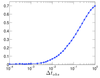
Figure 1: Proportion of incidences when the variance constraint is switched on and ${\bf{R}}_{\rm{w}}$ is positive definite as a function of the observation interval $\Delta t_{\rm{obs}}$ for the stochastic linear toy model (12). We used $\gamma_{x}=1$, $\gamma_{y}=1$, $\sigma_{x}=1$, $\sigma_{y}=1$, $\lambda=0.2$. We used $k=20$ ensemble members, 100 realizations and ${\bf{R}}_{\rm{o}}={\bf{H}}\bm{\Sigma}_{\rm clim}{\bf{H}}^{T}$ and no inflation with $\delta=1$. The analytically calculated critical observation interval according to equation (16) is $\Delta t_{\rm{obs}}=10^{-2}$.

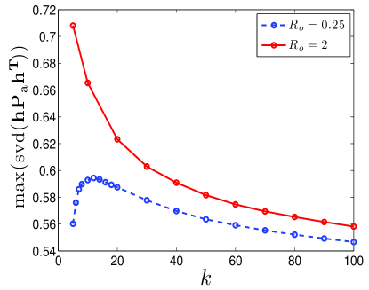
Figure 2: Average maximal singular value of ${\bf{h}}{\bf{P}}_{a}{\bf{h}}^{T}$ as a function of ensemble size $k$ for the stochastic linear toy model (12) using standard ETKF without inflation, with ${\bf{R}}_{\rm{o}}=0.25$ (dashed curve) and ${\bf{R}}_{\rm{o}}=2$ (solid curve). Parameters are $\sigma_{x}=\sigma_{y}=\gamma_{x}=\gamma_{y}=1$, $\lambda=0.2$, $\Delta t_{\rm{obs}}=1$, for which the climatic variance is ${\bf{h}}\Sigma{\bf{h}}^{T}\approx 0.505$. We used $50$ realizations for the averaging.

However, the fact that the variance constraint is switched on does not necessarily imply that the variance limiting filter will perform better than the standard ETKF. In particular, for very large observation intervals $\Delta t_{\rm{obs}}$ when the ensemble will have acquired the climatic mean and covariances, VLKF and ETKF will have equal skill. We now turn to the question under what conditions VLKF is expected to yield improved skill compared to standard ETKF. To this end we introduce as skill indicator the (squared) RMS error

$${\cal{E}}=\mathbb{E}^{t,dW}\|{\bar{{\bf{z}}}}_{a}(t_{i})-{\bf{z}}_{\rm{truth}}(t_{i})\|_{\bf G}^{2}\;,$$ (17)

between the truth ${\bf{z}}_{\rm{truth}}$ and the ensemble mean analysis ${\bar{{\bf{z}}}}_{a}$ (the square root is left out here for convenience of exposition). Here $\mathbb{E}^{t}$ denotes the temporal average over analyzes cycles, and $\mathbb{E}^{dW}$ denotes averaging over different realizations of the Brownian paths $dW$. We introduced the norm $\|{\bf{a}}{\bf{b}}\|_{\bf G}={\bf{a}}^{T}{\bf{G}}{\bf{b}}$ to investigate the overall skill using $\bf{G}={\bf{I}}$, the skill of the observed variables using ${\bf{G}}={\bf{H}}^{T}{\bf{H}}$ and the skill of the pseudo-observables using ${\bf{G}}={\bf{h}}^{T}{\bf{h}}$. Using the Kalman filter equation (3) for the analysis mean with ${\bf{K}}_{\rm{w}}=0$, we obtain for the ETKF

$${\cal{E}}^{\rm ETKF}=\mathbb{E}^{t,dW}\|({\bf{I}}-{\bf{K}}_{\rm{o}}{\bf{H}})({\bar{{\bf{z}}}}_{f}(t_{i})-{\bf{z}}_{\rm{truth}}(t_{i}))+{\bf{K}}_{\rm{o}}{\bf{r}}_{\rm{o}}(t_{i})\|_{\bf G}^{2}\;.$$

Solving the linear toy-model (12) for each member of the ensemble and then performing an ensemble average, we obtain

$${\bar{{\bf{z}}}}_{f}(t_{i})={\bm{L}}(\Delta t_{\rm{obs}})\;{\bar{{\bf{z}}}}_{a}(t_{i-1})\;.$$ (18)

Substituting a particular realization of the truth ${\bf{z}}_{\rm{truth}}(t)$, and performing the average over the realizations, we finally arrive at

$${\cal{E}}^{\rm ETKF}=\mathbb{E}^{t}\|({\bf{I}}-{\bf{K}}_{\rm{o}}{\bf{H}}){\bm{L}}(\Delta t_{\rm{obs}})\;\bm{\xi}_{t_{i-1}}\|_{\bf G}^{2}+\mathbb{E}^{t}\|({\bf{I}}-{\bf{K}}_{\rm{o}}{\bf{H}})\bm{\eta}_{t_{i}}\|_{\bf G}^{2}+\mathbb{E}^{t}\|{\bf{K}}_{\rm{o}}{\bf{r}}_{\rm{o}}\|_{\bf G}^{2}\;,$$ (19)

with the mutually independent normally distributed random variables

$$\bm{\xi}_{t_{i}} = {\bar{{\bf{z}}}}_{a}(t_{i})-{\bf{z}}_{\rm{truth}}(t_{i})\sim{\cal{N}}(0,{\bf{P}}_{a}(t_{i}))$$

$$\bm{\eta}_{t_{i}} = {\bm{\sigma}}\int_{t_{i-1}}^{t_{i}}{\bm{L}}(\Delta t_{\rm{obs}}-s)\,d{\bm{W}}_{s}\sim{\cal{N}}(0,\bm{\Sigma}(\Delta t_{\rm{obs}}))$$

$${\bf{r}}_{\rm{o}} \sim {\cal{N}}(0,{\bf{R}}_{\rm{o}})\;.$$ (20)

We have numerically verified the validity of our assumptions of the statistics of $\bm{\xi}_{t_{i}}$ and $\bm{\eta}_{t_{i}}$. Note that for $\bm{\xi}_{t_{i}}$ to have mean zero and variance ${\bf{P}}_{a}(t_{i})$ filter divergence has to be excluded. Similarly we obtain for the VLKF

$${\cal{E}}^{\rm VLKF} = \mathbb{E}^{t}\|({\bf{I}}-{\bf{K}}_{\rm{o}}{\bf{H}}){\bm{L}}(\Delta t_{\rm{obs}})\;\bm{\xi}_{t_{i-1}}\|_{\bf G}^{2}+\mathbb{E}^{t}\|({\bf{I}}-{\bf{K}}_{\rm{o}}{\bf{H}})\bm{\eta}_{t_{i}}\|_{\bf G}^{2}+\mathbb{E}^{t}\|{\bf{K}}_{\rm{o}}{\bf{r}}_{\rm{o}}\|_{\bf G}^{2}$$ (21)

$$+ \mathbb{E}^{t}\|{\bf{K}}_{\rm{w}}{\bf{h}}\bm{\zeta}_{t_{i}}\|_{\bf G}^{2}+2\,\mathbb{E}^{t}[({\bf{I}}-{\bf{K}}_{\rm{o}}{\bf{H}}){\bm{L}}(\Delta t_{\rm{obs}})\;\bm{\xi}_{t_{i-1}})^{T}\,{\bf{G}}\,({\bf{K}}_{\rm{w}}{\bf{h}}\;\bm{\zeta}_{t_{i}})]\;,$$

with the normally distributed random variable

$$\bm{\zeta}_{t_{i}} = {\bar{{\bf{z}}}}_{f}(t_{i})\sim{\cal{N}}(0,\frac{1}{k}{\bf{P}}_{f}(t_{i}))\;,$$ (22)

where we used that ${\bf{a}}_{\rm{clim}}=0$. Note that using our stationarity assumption to calculate ${\bf{P}}_{f}$ we have $\zeta_{t_{i}}\,{\buildrel d\over{\sim}}\,(1/k)\xi_{t_{i-1}}$. Again we have numerically verified the statistics for $\bm{\zeta}_{t_{i}}$. The expression for the RMS error of the VLKF (21) can be considerably simplified. Since for large ensemble sizes $k\to\infty$ the random variable $\zeta_{t_{i}}$ becomes a deterministic variable with mean zero, we may neglect all terms containing $\zeta_{t_{i}}$. We summarize to

$${\cal{E}}^{\rm VLKF}=\mathbb{E}^{t}\|({\bf{I}}-{\bf{K}}_{\rm{o}}{\bf{H}}){\bm{L}}(\Delta t_{\rm{obs}})\;\bm{\xi}_{t_{i-1}}\|_{\bf G}^{2}+\mathbb{E}^{t}\|({\bf{I}}-{\bf{K}}_{\rm{o}}{\bf{H}})\bm{\eta}_{t_{i}}\|_{\bf G}^{2}+\mathbb{E}^{t}\|{\bf{K}}_{\rm{o}}{\bf{r}}_{\rm{o}}\|_{\bf G}^{2}\;.$$ (23)

For convenience we have omitted superscripts for ${\bf{K}}_{\rm{o}}$ and $\bm{\xi}_{t_{i-1}}$ in (19) and (23) to denote whether they have been evaluated for ETKF and VLKF. But note that, although the expressions (19) and (23) are formally the same, one generally has ${\cal{E}}^{\rm ETKF}\neq{\cal{E}}^{\rm VLKF}$, because the analysis covariance matrices ${\bf{P}}_{a}$ are calculated differently for both methods leading to different gain matrices ${\bf{K}}_{\rm{o}}$ and different statistics of $\bm{\xi}_{t}$ in (19) and (23).

We can now estimate the skill improvement defined as

$${\cal{S}}={\cal{E}}^{\rm ETKF}/{\cal{E}}^{\rm VLKF}$$

with values of ${\cal{S}}>1$ indicating skill improvement of VLKF over ETKF. We shall choose ${\bf{G}}={\bf{h}}^{T}{\bf{h}}$ from now on, and concentrate on the skill improvement for the pseudo-observables. Recalling that ${\cal{E}}^{\rm ETKF}\approx{\cal{E}}^{\rm VLKF}$ for large observation intervals $\Delta t_{\rm{obs}}$, we expect skill improvement for small $\Delta t_{\rm{obs}}$. We perform again a Taylor expansion in small $\Delta t_{\rm{obs}}$ of the skill improvement ${\cal{S}}$. The resulting analytical expressions are very lengthy and cumbersome, and are therefore omitted for convenience.
We found that there is indeed skill improvement ${\cal{S}}>1$ in the limit of either $\gamma_{y}\to\infty$ or $\gamma_{x}\to 0$. This suggests that the skill is controlled by the ratio of the time scales of the observed and the unobserved variables. If the time scale of the pseudo-observables is much larger than the one of the observed variables, VLKF will exhibit superior performance over ETKF. This can be intuitively understood since $1/(2\gamma_{y})$ is the time scale on which equilibrium – i.e. the climatic state – is reached for the pseudo-observables ${\bf{y}}$. If the pseudo-observables have relaxed towards equilibrium within the observation interval $\Delta t_{\rm{obs}}$, and their variance has acquired the climatic covariance ${\bf{h}}{\bf{P}}_{a}{\bf{h}}^{T}=\bm{\sigma}_{\rm clim}^{2}$, we expect the variance limiting to be beneficial.

Furthermore, we found analytically that the skill improvement increases with increasing observational noise $R_{\rm obs}$ (at least in the small observation interval approximation). In particular we found that $\partial{\cal{S}}/\partial R_{\rm obs}>0$ at $R_{\rm obs}=0$. The increase of skill with increasing observational noise can be understood phenomenologically in the following way. For $R_{\rm obs}=0$ the filter trusts the observations, which as a time series carry the climatic covariance. This implies that there is a realization of the Wiener process such that the analysis can be reproduced by a model with the true values of $\gamma_{x,y}$ and $\sigma_{x,y}$. Similarly, this is the case in the other extreme $R_{\rm obs}\to\infty$, where the filter trusts the model. For $0\ll R_{\rm obs}\ll\infty$ the analysis reproducing system would have a larger covariance $\sigma_{x}$ than the true value. This slowed down relaxation towards equilibrium of the observed variables can be interpreted as an effective decrease of the damping coefficient $\gamma_{x}$. This effectively increases the time scale separation between the observed and the unobserved variables, which was conjectured above to be beneficial for skill improvement.

As expected, the skill improves with increasing inflation factor $\delta>1$. The improvement is exactly linear for $\Delta t_{\rm{obs}}\to 0$. This is due to the variance inflation leading to an increase of instances with ${\bf{h}}{\bf{P}}_{a}{\bf{h}}^{T}>\bm{\sigma}_{\rm clim}^{2}$, for which the variance constraint will be switched on.

In Figure 3 we present a comparison of the analytical results (19) and (23) with results from a numerical implementation of ETKF and VLKF for varying damping coefficient $\gamma_{y}$. Since $\gamma_{y}$ controls the time-scale of the ${\bf{y}}$-process, we cannot use the same $\Delta t_{\rm{obs}}$ for a wide range of $\gamma_{y}$ in order not to violate the small observation interval approximations used in our analytical expressions. We choose $\Delta t_{\rm{obs}}$ as a function of $\gamma_{y}$ such that the singular values of the first-order approximation of the forecast variance is a good approximation for this $\Delta t_{\rm{obs}}$. For Figure 3 we have $\Delta t_{\rm{obs}}\in(0.005,0.01)$ to preserve the validity of the Taylor expansion. Besides the increase of the skill with $\gamma_{y}$, Figure 3 shows that the value of ${\cal{S}}$ increases significantly for larger values of the inflation factor $\delta>1$.

We will see in the next Section that the results we obtained for the simple linear toy model (12) hold as well for a more complicated higher-dimensional model, where the dynamic Brownian driving noise is replaced by nonlinear chaotic dynamics.

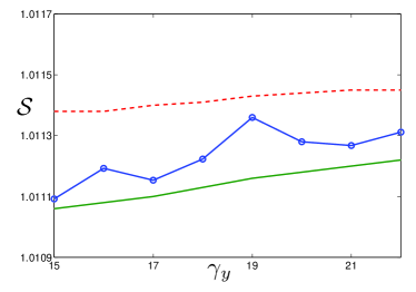
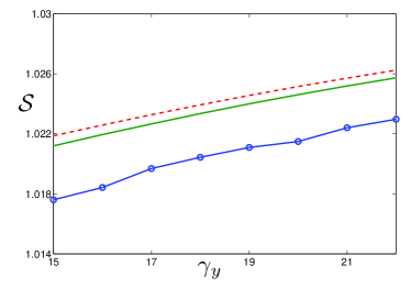
Figure 3: Dependency of the skill improvement ${\cal{S}}$ of VLKF over ETKF on the damping coefficient $\gamma_{y}$ of the pseudo-observable. We show a comparison of direct numerical simulations (open circles) with analytical results using (21) (continuous curve) and the approximation of large ensemble size (23) (dashed curve). Parameters are $\gamma_{x}=1$, $\lambda=2$, $\sigma_{x}=\sigma_{y}=1$, $R_{\rm obs}=0.25$. We used an ensemble size of $k=20$ and averaged over $1000$ realizations. Left: no inflation with $\delta=1$. Right: Inflation with $\delta=1.02^{2}$.

5 Numerical results for the Lorenz-96 system

We illustrate our method with the Lorenz-96 system (Lorenz, 1996) and show its usefulness for sparse observations in improving the analysis skill and stabilizing the filter. In (Lorenz, 1996) Lorenz proposed the following model for the atmosphere

$${\dot{z}}_{i}=z_{i-1}(z_{i+1}-z_{i-2})-z_{i}+F\qquad i=1,\cdots,D$$ (24)

with ${\bf{z}}=(z_{1},\cdots,z_{D})$ and periodic $z_{i+D}=z_{i}$. This system is a toy-model for midlatitude atmospheric dynamics, incorporating linear damping, forcing and nonlinear transport. The dynamical properties of the Lorenz-96 system have been investigated, for example, in (Lorenz and Emanuel, 1998; Orrell and Smith, 2003; Gottwald and Melbourne, 2005), and in the context of data assimilation it was investigated in, for example, (Ott et al., 2004; Fisher et al., 2005; Harlim and Majda, 2010). We use $D=40$ modes and set the forcing to $F=8$. These parameters correspond to a strongly chaotic regime (Lorenz, 1996). For these parameters one unit of time corresponds to $5$ days in the earth’s atmosphere as calculated by calibrating the $e$-folding time of the asymptotic growth rate of the most unstable mode with a time scale of $2.1$ days (Lorenz, 1996). Assuming the length of a midlatitude belt to be about $30,000$km, the spatial scale corresponding to a discretization of the circumference of the earth along the midlatitudes in $D=40$ grid points corresponds to a spacing between adjacent grid points $z_{i}$ of approximately $750$km, roughly equalling the Rossby radius of deformation at midlatitudes. We estimated from simulations the advection velocity to be approximately $10.4$ m/sec which compares well with typical wind velocities in the midlatitudes.

In the following we will investigate the effect of using VLKF on improving the analysis skill when compared to a standard ensemble transform Kalman filter, and on stabilizing the filter and avoiding blow-up as discussed in (Ott et al., 2004; Kepert, 2004; Harlim and Majda, 2010). We perform twin experiments using a $k=41$-member ETKF and VLKF with the same truth time series, the same set of observations and the same initial ensemble. We have chosen an ensemble with $k>D$ in order to eliminate the effect that a finite-size ensemble can only fit as many observations as the number of its ensemble members (Lorenc, 2003). Here we want to focus on the effect of limiting the variance.

The system is integrated using the implicit mid-point rule (see for example Leimkuhler and Reich (2005)) to a time $T=30$ with a time step $dt=1/240$. The total time of integration corresponds to an equivalent of $150$ days, and the integration timestep $dt$ corresponds to half an hour. We measured the approximate climatic mean and variance, $\mu_{\rm{clim}}$ and $\sigma_{\rm{clim}}^{2}$, respectively, via a long time integration over a time interval of $T=2000$ which corresponds roughly to $27.5$ years. Because of the symmetry of the system (24), the mean and the standard deviation are the same for all variables $z_{i}$, and are measured to be $\sigma_{\rm{clim}}=3.63$ and $\mu_{\rm{clim}}=2.34$.

The initial ensemble at $t=0$ is drawn from an ensemble with variance $\sigma_{\rm{clim}}^{2}$; the filter was then subsequently spun up for sufficiently many analysis cycles to ensure statistical stationarity. We assume Gaussian observational noise of the order of $25$% of the climatological standard deviation $\sigma_{clim}$, and set the observational error covariance matrix ${\bf{R}}_{\rm{o}}=(0.25\sigma_{clim})^{2}\,\mathbf{I}$. We find that for larger observational noise levels the variance limiting correction (11) is used more frequently. This is in accordance with our finding in the previous section for the toy model.

We study first the performance of the filter and its dependence on the time between observations $\Delta t_{\rm{obs}}$ and the proportion of the system observed $1/N_{\rm{obs}}$. $N_{\rm{obs}}=2$ means only every second variable is observed, $N_{\rm{obs}}=4$ only every fourth, and so on.

We have used a constant variance inflation factor $\delta=1.05$ for both filters. We note that the optimal inflation factor at which the RMS error $\cal{E}$ is minimal, is different for VLKF and ETKF. For $\Delta t_{obs}=5/120$ ($5$ hours) and $N_{obs}=4$ we find that $\delta=1.06$ produces minimal RMS errors for VLKF and $\delta=1.04$ produces minimal RMS errors for ETKF. For $\delta<1.04$ filter divergence occurs in ETKF, so we chose $\delta=1.05$ as a compromise between controlling filter divergence and minimizing the RMS errors of the analysis.

Figure 4 shows a sample analysis using ETKF with $N_{obs}=5$, $\Delta t_{\rm{obs}}=0.15$ and ${\bf{R}}_{\rm{o}}=(0.25\sigma_{clim})^{2}\,\mathbf{I}$ for an arbitrary unobserved component (top panel) and an arbitrary observed component (bottom panel) of the Lorenz-96 model. While the figure shows that the analysis (continuous grey line) tracks the truth (dashed line) reasonably well for the observed component, the analysis is quite poor for the unobserved component. Substantial improvements are seen for the VLKF when we incorporate information about the variance of the un-observed pseudo-observables, as can be seen in Figure 5. We set the mean and the variance of the pseudo-observables to be the climatic mean and variance, ${\bf{a}}_{\rm{clim}}=\mu_{\rm{clim}}{\bf e}$ and ${\bf{A}}_{\rm{clim}}=\sigma_{\rm clim}^{2}{\bf I}$ to filter the same truth with the same observations as used to produce Fig. 4. For these parameters (and in this realization) the quality of the analysis in both the observed and unobserved components is improved.

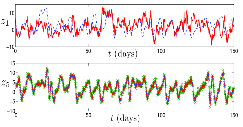
Figure 4: Sample ETKF analysis (continuous grey line) for observed $z_{5}$ (bottom panel) and unobserved $z_{1}$ (top panel) component. The dashed line is the truth, the crosses are observations. Parameters used were $N_{obs}=5$, $\Delta t_{\rm{obs}}=0.15$ (18 hours) and ${\bf{R}}_{\rm{o}}=(0.25\sigma_{clim})^{2}\,\mathbf{I}$.

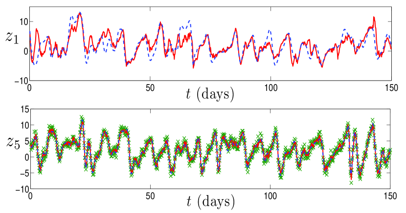
Figure 5: Sample VLKF analysis (continuous grey line) for observed $z_{5}$ (bottom panel) and unobserved $z_{1}$ (top panel) component. The dashed line is the truth, the crosses are observations. Parameters as in Figure 4.

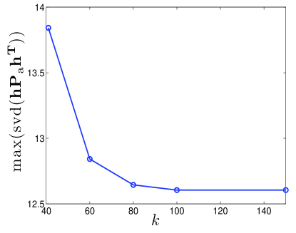
Figure 6: Average maximal singular value of ${\bf{h}}{\bf{P}}_{a}{\bf{h}}^{T}$ as a function of ensemble size $k$ for the Lorenz-96 model (24), using standard ETKF without inflation. All other parameters are as in Figure 4. We used $150$ realisations for the averaging.

As for the linear toy model (12), finite ensemble sizes exacerbate the overestimation of error covariances. In Figure 6 the maximal singular value of ${\bf{h}}{\bf{P}}_{a}{\bf{h}}^{T}$, averaged over $150$ realizations, is shown for ETKF as a function of ensemble size $k$. Again we use no inflation, i.e. $\delta=1$, in order to focus on the effect of finite ensemble sizes. The projected covariance clearly decreases for large enough ensemble sizes. However, here the limit of the maximal singular value of ${\bf{h}}{\bf{P}}_{a}{\bf{h}}^{T}$ for $k\to\infty$ underestimates the climatic variance $\sigma_{\rm{clim}}^{2}=13.18$.

To quantify the improvement of the VLKF filter we measure the site-averaged RMS error

$${\cal{E}}=\sqrt{\langle\frac{1}{LD_{o}}\sum_{l=1}^{L}\|{\bar{{\bf{z}}}}_{a}(l\Delta t_{\rm{obs}})-{\bf{z}}_{\rm{truth}}(l\Delta t_{\rm{obs}})\|^{2}\rangle}$$ (25)

between the truth ${\bf{z}}_{\rm{truth}}$ and the ensemble mean ${\bar{{\bf{z}}}}_{a}$ with $L=\lfloor T/\Delta t_{\rm{obs}}\rfloor$ where the average is taken over $500$ different realizations, and $D_{o}\leq D$ denotes the length of the vectors ${\bar{{\bf{z}}}}_{a}$. In tables 1 we display ${\cal{E}}$ for the ETKF and VLKF respectively, as a function of $N_{obs}$ and $\Delta t_{\rm{obs}}$. The increased RMS error for larger observation intervals $\Delta t_{\rm{obs}}$ can be linked to the increased variance of the chaotic nonlinear dynamics generated during longer integration times between analyses. Figure 7 shows the average proportional improvement of the VLKF over ETKF, obtained from the values of tables 1. Figure 7 shows that the skill improvement is greatest when the system is observed frequently. For large observation intervals $\Delta t_{\rm{obs}}$ ETKF and VLKF yield very similar RMS. We checked that for large observation intervals $\Delta t_{\rm{obs}}$ both filters still produce tracking analyses. Note that the observation intervals $\Delta t_{\rm{obs}}$ considered here are all much smaller than the $e$-folding time of $2.1$ days. The most significant improvement occurs when one quarter of the system is observed, that is for $N_{obs}=4$, and for small observation intervals $\Delta t_{\rm{obs}}$. The dependency of the skill of VLKF on the observation interval is consistent with our analytical findings in Section 4.

We have tested that the increase in skill as depicted in Figure 7 is not sensitive to incomplete knowledge of the statistical properties of the pseudo-observables by perturbing ${\bf{A}}_{\rm{clim}}$ and ${\bf{a}}_{\rm{clim}}$ and then monitoring the change in RMS error. We performed simulations where we drew ${\bf{A}}_{\rm{clim}}$ and ${\bf{a}}_{\rm{clim}}$ independently from uniform distributions $(0.9\,{\bf{A}}_{\rm{clim}},1.1\,{\bf{A}}_{\rm{clim}})$ and $(0.9\,{\bf{a}}_{\rm{clim}},1.1\,{\bf{a}}_{\rm{clim}})$. We found that for parameters $N_{obs}=2,4,6$, $\eta=0.05,0.25,0.5$ (with $\eta$ measuring the amount of the climatic variance used through ${\bf{R}}_{\rm{o}}=(\eta\,\sigma_{clim})^{2}\,\mathbf{I}$), and $\Delta t_{\rm{obs}}=0.025,0.05,0.25$ (corresponding to $3$, $6$ and $30$ hours) over a number of simulations there was on average no more than 7% difference of the analysis mean and the singular values of the covariance matrices between the control run where ${\bf{A}}_{\rm{clim}}=\sigma_{\rm clim}^{2}{\bf I}$ and ${\bf{a}}_{\rm{clim}}=\mu_{\rm{clim}}{\bf e}$ is used, and when ${\bf{A}}_{\rm{clim}}$ and ${\bf{a}}_{\rm{clim}}$ are simultaneously perturbed.

An interesting question is how the relative skill improvement is distributed over the observed and unobserved variables. This is illustrated in Figure 8 and Figure 9. In Figure 8 we show the proportional skill improvement of VLKF over ETKF for the observed variables and the pseudo-observables, respectively. Figure 8 shows that the skill improvement is larger for the pseudo-observables than for the observables which is to be expected. In Figure 9 we show the actual RMS error ${\cal{E}}$ for ETKF and VLKF for the observed variables and the pseudo-observables. It is shown that the skill improvement is better for the unobserved pseudo-observables for all observation intervals $\Delta t_{\rm{obs}}$. In contrast, VLKF exhibits an improved skill for the observed variables either for small observation intervals for all values of $N_{\rm{obs}}$ or for all (sufficiently small) observation intervals when $N_{\rm{obs}}=4,5$. We have, however, checked that the analysis is still tracking the truth reasonably well, and the discrepancy with ETKF is not due to the analysis not tracking the truth anymore. As expected, the RMS error asymptotes for large observation intervals $\Delta t_{\rm{obs}}$ (not shown) to the standard deviation of the observational noise $0.25\,\sigma_{\rm{clim}}\approx 0.91$ for the observables, and to the climatic standard deviation $\sigma_{\rm{clim}}=3.63$ for the pseudo-observable (not shown), albeit slightly reduced for small values of $N_{\rm{obs}}$ due to the impact of the surrounding observed variables (see Figure 10).

Note that there is an order of magnitude difference between the RMS errors for the observables and the pseudo-observables for large $N_{\rm{obs}}$ (cf. Figures 9). This suggests that the information of the observed variables does not travel too far away from the observational sites. However, the nonlinear coupling in the Lorenz-96 system (24) allows for information of the observed components to influence the error statistics of the unobserved components. Therefore the RMS error of pseudo-observables adjacent to observables are better than those far away from observables. Moreover, the specific structure of the nonlinearity introduces a translational symmetry-breaking (one may think of the nonlinearity as a finite difference approximation of an advection term ${\bf{z}}{\bf{z}}_{x}$), which causes those pseudo-observables to the right of an observable to have a more reduced RMS error than those to the left of an observable. This is illustrated in Figure 10 where the RMS error is shown for each site when only one site is observed. The advective time scale of the Lorenz-96 system is much smaller than $\Delta t_{\rm{obs}}$ which explains why the skill is not equally distributed over the sites, and why, especially for large values of $N_{\rm{obs}}$, we observe a big difference between the site-averaged skills of the observed and unobserved variables.

$N_{obs}$	6	4.40	3.64	3.42	3.32	3.29	3.30	3.30	3.28	3.26	3.26
	5	4.08	2.88	2.70	2.83	3.02	3.07	3.17	3.21	3.19	3.20
	4	2.42	1.17	1.35	1.72	2.18	2.37	2.62	2.84	2.98	3.06
	3	0.49	0.51	0.60	0.71	0.89	1.11	1.38	1.68	2.02	2.25
	2	0.31	0.34	0.38	0.43	0.49	0.55	0.66	0.75	0.90	1.13
	1	0.19	0.21	0.24	0.26	0.29	0.31	0.33	0.36	0.39	0.44
		0.025	0.05	0.075	0.1	0.125	0.15	0.175	0.2	0.225	0.25
		3 h	6 h	9 h	12 h	15 h	18 h	21 h	24 h	27 h	30 h
		$\Delta t_{\rm{obs}}$
$N_{obs}$	6	3.20	3.09	3.10	3.15	3.20	3.22	3.27	3.27	3.26	3.27
	5	2.73	2.28	2.51	2.70	2.89	3.03	3.07	3.14	3.15	3.15
	4	1.30	1.03	1.28	1.66	2.04	2.29	2.55	2.70	2.88	2.96
	3	0.48	0.51	0.59	0.70	0.87	1.07	1.39	1.71	1.95	2.21
	2	0.31	0.34	0.38	0.44	0.50	0.56	0.64	0.77	0.95	1.14
	1	0.19	0.21	0.24	0.26	0.29	0.31	0.33	0.36	0.39	0.44
		0.025	0.05	0.075	0.1	0.125	0.15	0.175	0.2	0.225	0.25
		3 h	6 h	9 h	12 h	15 h	18 h	21 h	24 h	27 h	30 h
		$\Delta t_{\rm{obs}}$

Table 1: RMS errors for ETKF (upper table) and VLKF (bottom table), averaged over 500 simulations, and with ${\bf{R}}_{\rm{o}}=(0.25\sigma_{clim})^{2}\,\mathbf{I}$ as observational noise.

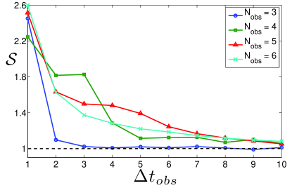
Figure 7: Proportional skill improvement of VLKF over ETKF as a function of the observation interval $\Delta t_{\rm{obs}}$ for different values of $N_{\rm{obs}}$, with observational noise ${\bf{R}}_{\rm{o}}=(0.25\sigma_{clim})^{2}\,\mathbf{I}$. A total of $500$ simulations were used to perform the ensemble average in the RMS errors ${\cal{E}}$ using (25) for ETKF and VLKF. $\Delta t_{\rm{obs}}$ is measured in hours.

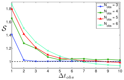
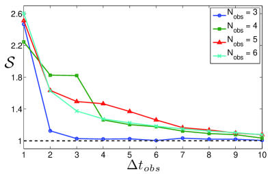
Figure 8: Proportional skill improvement of VLKF over ETKF as a function of the observation interval $\Delta t_{\rm{obs}}$ for different values of $N_{\rm{obs}}$. The RMS error ${\cal{E}}$ is calculated using only the observed variables (left) or only the pseudo-observables (right). $\Delta t_{\rm{obs}}$ is measured in hours. Parameters as in Figure 7.

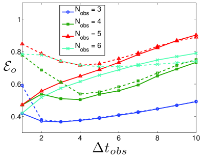
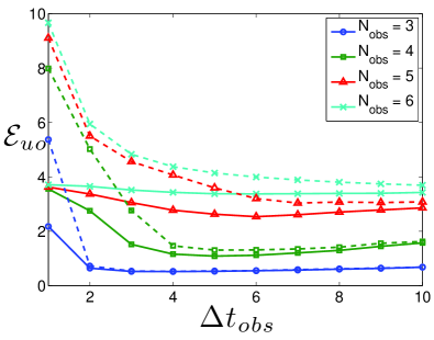
Figure 9: RMS error of VLKF (solid lines) and ETKF (dashed lines) for ${\bf{R}}_{\rm{o}}=(0.25\sigma_{clim})^{2}\,\mathbf{I}$, where ${\cal{E}}$ is calculated using only the observed variables (left) or only the pseudo-observables (right). $\Delta t_{\rm{obs}}$ is measured in hours. Parameters as in Figure 7.

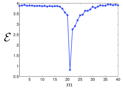
Figure 10: RMS error ${\cal{E}}$ for each variable $z_{i}$ as a function of the lattice site $i$. Only one observable was used at $i=21$. Time between observations is $\Delta t_{\rm{obs}}=10$ hours and observational noise with covariance ${\bf{R}}_{\rm{o}}=(0.25\,\sigma_{clim}^{2}){\bf{I}}$ was used. The results are averaged over $100$ different realizations.

In Figure 11 we show how the RMS error behaves as a function of the observational noise level. We see that for $N_{\rm{obs}}=4$ VLKF always has a smaller RMS error than ETKF.

The results confirm again the results from our analysis of the toy model in Section 4, that VLKF yields best performance for small observation intervals $\Delta t_{\rm{obs}}$ and for large noise levels. For large observation intervals ETKF and VLKF perform equally well, since then the chaotic model dynamics will have lead the ensemble to have acquired the climatic variance during the time of propagation.

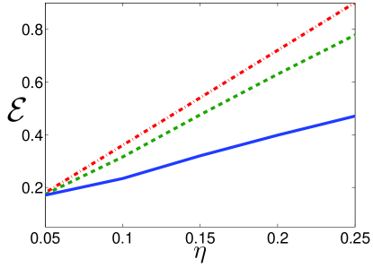
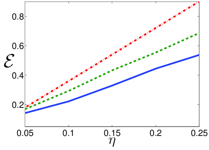
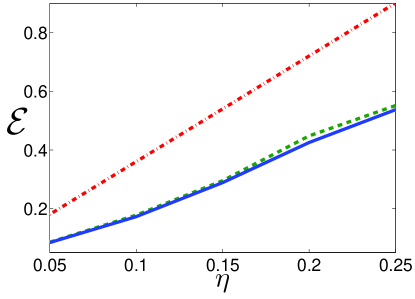
Figure 11: RMS error $\cal{E}$ of VLKF (solid lines) and ETKF (dashed lines), as a function of the observational noise, measured here by $\eta$ defined via ${\bf{R}}_{\rm{o}}=(\eta\,\sigma_{clim})^{2}\,\mathbf{I}$. The dotted line indicates the RMS error if only observations were used. We show results from top to bottom for several observation intervals: $\Delta t_{\rm{obs}}=1$ hour, $\Delta t_{\rm{obs}}=2$ hours and $\Delta t_{\rm{obs}}=5$ hours. $N_{\rm{obs}}=4$ was used and $1000$ simulations were carried out to perform the ensemble averages in the RMS errors ${\cal{E}}$ using (25) for ETKF and VLKF.

In (Ott et al., 2004) it was observed that if not all variables $z_{i}$ are observed the Kalman filter diverges exhibiting blow-up. Similar behaviour was observed in (Harlim and Majda, 2010). In (Ott et al., 2004) the authors suggested that the sparsity of observations leads to an inhomogeneous background error, which causes an underestimation of the error covariance. We study here this catastrophic blow-up divergence (as opposed to filter divergence when the analysis diverges from the truth) and its dependence on the time between observations $\Delta t_{\rm{obs}}$ and the proportion of the system observed $1/N_{\rm{obs}}$. We note that blow-up divergence appears only in the case of sufficiently small observational noise and moderate values of $\Delta t_{\rm{obs}}$. Once $\Delta t_{\rm{obs}}$ is large enough (in fact, larger than the $e$-folding time corresponding to the most unstable Lyapunov exponent, in our case $2.1$ days) we notice that no catastrophic divergence occurs, independent of $N_{\rm{obs}}$. This probably occurs because for large observation intervals the ensemble acquires enough variance through the nonlinear propagation. We prescribe Gaussian observational noise of the order of $5$% of the climatological standard deviation $\sigma_{clim}$, and set the observational error covariance matrix to ${\bf{R}}_{\rm{o}}=(0.05\,\sigma_{clim})^{2}\,\mathbf{I}$. The initial ensemble at $t=0$ is drawn again from an ensemble with variance $\sigma_{\rm{clim}}^{2}$.

To study the performance of VLKF when blow-up occurs in ETKF simulations we count the number $N_{b}$ of blow-ups that occur before a total of $100$ simulations have terminated without blow-up. The proportions of blow-ups for the respective filters is then given by $N_{b}/(N_{b}+100)$. We tabulate this proportion in tables 2 for the ETKF and VLKF respectively and the proportional improvement in table 3. The ‘x’s’ in the table represent cases where no successful simulations could be obtained due to blow-up.

Both filters suffer from severe filter instability for $N_{\rm{obs}}=6$, i.e. for very sparse observational networks, at small observation intervals $\Delta t_{\rm{obs}}$. No blow-up occurs for either filter when every variable is observed. Note the reduction in occurrences of blow-ups for large observation intervals $\Delta t_{\rm{obs}}$ as discussed above. We have checked that for all $N_{\rm{obs}}$ there is no blow-up for ETKF (and VLKF) for sufficiently large $\Delta t_{\rm{obs}}$ (not shown); the larger $N_{\rm{obs}}$ the smaller the upper bound of $\Delta t_{\rm{obs}}$ such that no blow-ups occur. Collapse is most prominent for ETKF (and for VLKF, but to a much lesser extent) for larger values of $N_{\rm{obs}}$ and at intermediate observation intervals which depend on $N_{\rm{obs}}$. Tables 2 and 3 clearly show that incorporating information about the pseudo-observables strongly increases the stability of the filter and suppresses blow-up. However, we note that despite the gain in stability VLKF has a skill less than the purely observational skill in the cases when blow-up occurs for ETKF, because the solutions become non-tracking. Further research is under way to improve on this in the VLKF framework.

$N_{obs}$	6	0.14	x	x	0.98	0.96	0.76	0.32	0.05	0.02	0.01
	5	0.02	0.40	0.67	0.73	0.84	0.89	0.94	0.82	0.49	0.19
	4	0	0.04	0.22	0.29	0.49	0.64	0.77	0.83	0.89	0.82
	3	0	0	0	0.03	0.04	0.11	0.15	0.44	0.58	0.67
	2	0	0	0	0	0	0.01	0	0.01	0.05	0.15
		0.025	0.05	0.075	0.1	0.125	0.15	0.175	0.2	0.225	0.25
		3 h	6 h	9 h	12 h	15 h	18 h	21 h	24 h	27 h	30 h
		$\Delta t_{\rm{obs}}$
$N_{obs}$	6	0.01	0.42	0.11	0.01	0	0	0	0	0	0
	5	0	0.24	0.36	0.10	0.01	0	0	0	0	0
	4	0	0.03	0.22	0.12	0.06	0.02	0	0	0	0
	3	0	0	0	0.02	0	0.01	0.01	0.01	0	0
	2	0	0	0	0	0	0	0	0	0	0.01
		0.025	0.05	0.075	0.1	0.125	0.15	0.175	0.2	0.225	0.25
		3 h	6 h	9 h	12 h	15 h	18 h	21 h	24 h	27 h	30 h
		$\Delta t_{\rm{obs}}$

Table 2: Proportion of catastrophically diverging simulations with ETKF (upper table) and VLKF (lower table). Observational noise with ${\bf{R}}_{\rm{o}}=(0.05\sigma_{clim})^{2}\,\mathbf{I}$ was used.

$N_{obs}$	6	14	x	x	98.00	$\infty$	$\infty$	$\infty$	$\infty$	$\infty$	$\infty$
	5	$\infty$	1.67	1.86	7.30	84.00	$\infty$	$\infty$	$\infty$	$\infty$	$\infty$
	4	1	1.33	1.00	2.42	8.17	32.00	$\infty$	$\infty$	$\infty$	$\infty$
	3	1	1	1	1.5	$\infty$	11.00	15.00	44.00	$\infty$	$\infty$
	2	1	1	1	1	1	$\infty$	1	$\infty$	$\infty$	15.00
		0.025	0.05	0.075	0.1	0.125	0.15	0.175	0.2	0.225	0.25
		3 h	6 h	9 h	12 h	15 h	18 h	21 h	24 h	27 h	30 h
		$\Delta t_{\rm{obs}}$

Table 3: Proportional improvement of VLKF and ETKF as calculated as the ratio of the values from tables 2.

The fact that incorporating information about the variance of the un-observed variables improves the stability of the filter is in accordance with the interpretation of filter divergence of sparse observational networks provided in (Ott et al., 2004).

6 Discussion

We have developed a framework to include information about the variance of unobserved variables in a sparse observational network. The filter is designed to control overestimation of error covariances typical in sparse observation networks, and limits the posterior analysis covariance of the unresolved variables to stay below their climatic variance. We have done so in a variational setting and found a relationship between the error covariance of the variance constraint ${\bf{R}}_{\rm{w}}$ and the assumed target variance of the unobserved pseudo-observables ${\bf{A}}_{\rm{clim}}$.

We illustrated the beneficial effects of the variance limiting filter in improving the analysis skill when compared to the standard ensemble square root Kalman filter. We expect the variance limiting constraint to improve data assimilation for ensemble Kalman filters when finite size effects of too small ensemble sizes overestimate the error covariances, in particular in sparse observational networks. In particular we found that the skill will improve for small observation intervals $\Delta t_{\rm{obs}}$ and sufficiently large observational noise. We found substantial skill improvement for both observed and unobserved variables. These effects can be understood with a simple linear toy model which allows for an analytical treatment. We further established numerically that VLKF reduces the probability of catastrophic filter divergence and improves the stability of the filter when compared to the standard ensemble square root Kalman filter.

We remark that the idea of the variance limiting Kalman filter is not restricted to ensemble Kalman filters but can also be used to modify the extended Kalman filter. However, for the examples we used here the nonlinearities were too strong and the extended Kalman filter did not yield satisfactory results, even in the variance limiting formulation.

The effect of the variance limiting filter to control unrealistically large error covariances of the poorly resolved variables due to finite ensemble sizes may find useful applications. We mention here that the variance constraint is able to adaptively damp unrealistic excitation of ensemble spread in underesolved spatial regions due to inappropriate uniform inflation. This may be an alternative to the spatially adaptive schemes which were recently developed (Anderson, 2007; Li et al., 2009). In addition, it is known that localization of covariance matrices in EnKF leads to imbalance in the analyzed fields (see, e.g., Houtekamer and Mitchell (2005); Kepert (2009) for a recent study). Filter localization typically excites unwanted gravity waves which when uncontrolled can substantially degrade filter performance. One may construct balance constraints as pseudo-observations and thereby potentially reduce this undesired aspect of covariance localization. As more specific applications, we mention climate reanalysis and data assimilation for the mesosphere. It would be interesting to see how the proposed variance limiting filter can be used in climate reanalysis schemes to deal with the vertical sparcity of observational data and the less dense observation network on the southern hemisphere in the pre-radiosonde era (see Whitaker et al. (2004)). One would need to establish though whether the historical observation intervals $\Delta t_{\rm{obs}}$ are sufficiently small to allow for a skill improvement. Similarly, it may help to control the dynamically dominant gravity wave activity in the mesosphere as the upper lid is pushed further and further (see for example Polavarapu et al. (2005)). However, a word of caution is required here. In some atmospheric data assimilation problems, it is not at all uncommon to have an ensemble prior variance for certain variables that is significantly larger than the climatological variance, when the atmosphere is locally far away from equilibrium. One relevant example would be in the vicinity of strong fronts over the southern ocean. In such a case, it may not be appropriate to limit the variance to the climatological value.

In this work we have studied systems where for sufficiently large observation intervals $\Delta t_{\rm{obs}}$ the variables acquire their true climatological mean and variance when the model is run. In particular we have not included model error. It would be interesting to see whether the variance limiting filter can help to control model error in the case that the free running model would produce unrealistically large forecast covariances. Usually numerical schemes do underestimate error covariances, but this is often caused by severe divergence damping (Durran, 1999) which is artificially introduced to the model to control unwanted gravity wave activity and to stabilize the numerical scheme. The stabiliziation may be achieved by a much smaller amount of divergence damping by implementing the variance limiting constraint in the data assimilation procedure. The VLKF would in this case act as an effective adaptive damping scheme, counteracting the model error.

References

- Anderson (2001) Anderson, J. L. (2001). An ensemble adjustment Kalman filter for data assimilation. Mon. Wea. Rev., 129, 2884–2903.
- Anderson (2007) Anderson, J. L. (2007). An adaptive covariance inflation error correction algorithm for ensemble filters. Tellus, 59A, 210–224.
- Anderson (2009) Anderson, J. L. (2009). Spatially and temporally varying adaptive covariance inflation for ensemble filters. Tellus, 61A, 72–83.
- Anderson and Anderson (1999) Anderson, J. L. and Anderson, S. L. (1999). A monte carlo implementation of the nonlinear filtering problem to produce ensemble assimilations and forecasts. Monthly Weather Review, 127(12), 2741–2758.
- Bengtsson et al. (2007) Bengtsson, L., Arkin, P., Berrisford, P., Bougeault, P., Folland, C. K., Gordon, C., Haines, K., Hodges, K. I., Jones, P., Kallberg, P., Rayner, N., Simmons, A., Stammer, D., Thorne, P. W., Uppala, S., and Vose, R. S. (2007). The need for a dynamical climate reanalysis. BAMS, 88(4), 495–501.
- Bergemann et al. (2009) Bergemann, K., Gottwald, G., and Reich, S. (2009). Ensemble propagation and continuous matrix factorization algorithms. Q. J. R. Meteorol. Soc., 135, 1560–1572.
- Bocquet et al. (2010) Bocquet, M., Pires, C. A., and Wu, L. (2010). Beyond gaussian statistical modeling in geophysical data assimilation. Monthly Weather Review, 138(8), 2997–3023.
- Buizza et al. (1999) Buizza, R., Miller, M., and Palmer, T. N. (1999). Stochastic representation of model uncertainties in the ECMWF Ensemble Prediction System. Q. J. R. Meteorol. Soc., 125(560), 2887–2908.
- Charron et al. (2010) Charron, M., Pellerin, G., Spacek, L., Houtekamer, P. L., Gagnon, N., Mitchell, H. L., and Michelin, L. (2010). Toward random sampling of model error in the canadian ensemble prediction system. Monthly Weather Review, 138(5), 1877–1901.
- Compo et al. (2011) Compo, G. P., Whitaker, J. S., Sardeshmukh, P. D., Matsui, N., Allan, R. J., Yin, X., Gleason, B. E., Vose, R. S., Rutledge, G., Bessemoulin, P., Brönnimann, S., Brunet, M., Crouthamel, R. I., Grant, A. N., Groisman, P. Y., Jones, P. D., Kruk, M. C., Kruger, A. C., Marshall, G. J., Maugeri, M., Mok, H. Y., Nordli, ., Ross, T. F., Trigo, R. M., Wang, X. L., Woodruff, S. D., and Worley, S. J. (2011). The twentieth century reanalysis project. Quarterly Journal of the Royal Meteorological Society, 137(654).
- Durran (1999) Durran, D. R. (1999). Numerical Methods for Wave Equations in Geophysical Fluid Dynamics. Springer, New York.
- Eckermann et al. (2009) Eckermann, S. D., Hoppel, K. W., Coy, L., McCormack, J. P., Siskind, D. E., Nielsen, K., Kochenash, A., Stevens, M. H., Englert, C. R., Singer, W., and Hervig, M. (2009). High-altitude data assimilation system experiments for the northern summer mesosphere season 2007. J. Atmos. and Solar-Terr. Phys., 71, 531–551.
- Ehrendorfer (2007) Ehrendorfer, M. (2007). A review of issues in ensemble-based Kalman filtering. Meteorologische Zeitschrift, 16(6), 795–818.
- Evensen (2006) Evensen, G. (2006). Data Assimilation: The Ensemble Kalman Filter. Springer, New York.
- Fisher et al. (2005) Fisher, M., Leutbecher, M., and Kelly, G. A. (2005). On the equivalence between Kalman smoothing and weak-constraint four-dimensional variational data assimilation. Q. J. R. Meteorol. Soc., 131, 3235–3246.
- Gardiner (2003) Gardiner, C. W. (2003). Handbook of Stochastic Methods for Physics, Chemistry, and the Natural Sciences. Springer, New York, 3rd edition.
- Golub and Loan (1996) Golub, G. H. and Loan, C. F. V. (1996). Matrix Computations. The Johns Hopkins University Press, Baltimore, 3rd edition.
- Gottwald and Melbourne (2005) Gottwald, G. A. and Melbourne, I. (2005). Testing for chaos in deterministic systems with noise. Physica D, 212, 100–110.
- Hamill and Whitaker (2005) Hamill, T. M. and Whitaker, J. S. (2005). Accounting for the error due to unresolved scales in ensemble data assimilation: A comparison of different approaches. Mon. Wea. Rev., 133, 3132–3147.
- Hamill et al. (2001) Hamill, T. M., Whitaker, J. S., and Snyder, C. (2001). Distance-dependent filtering of background covariance estimates in an ensemble Kalman filter. Mon. Wea. Rev., 129, 2776–2790.
- Harlim and Majda (2010) Harlim, J. and Majda, A. J. (2010). Catastrophic filter divergence in filtering nonlinear dissipative systems. Comm. Math. Sci., 8, 27–43.
- Houtekamer and Mitchell (1998) Houtekamer, P. L. and Mitchell, H. L. (1998). Data assimilation using an ensemble kalman filter technique. Monthly Weather Review, 126(3), 796–811.
- Houtekamer and Mitchell (2001) Houtekamer, P. L. and Mitchell, H. L. (2001). A sequential ensemble Kalman filter for atmospheric data assimilation. Mon. Wea. Rev., 129, 123–136.
- Houtekamer and Mitchell (2005) Houtekamer, P. L. and Mitchell, H. L. (2005). Ensemble kalman filtering. Q. J. R. Meteorol. Soc., 131, 3269–3289.
- Houtekamer et al. (2005) Houtekamer, P. L., Mitchell, H. L., Pellerin, G., Buehner, M., Charron, M., Spacek, L., and Hansen, B. (2005). Atmospheric data assimilation with an ensemble kalman filter: Results with real observations. Monthly Weather Review, 133(3), 604–620.
- Houtekamer et al. (2009) Houtekamer, P. L., Mitchell, H. L., and Deng, X. (2009). Model error representation in an operational ensemble kalman filter. Monthly Weather Review, 137(7), 2126–2143.
- Ide et al. (1997) Ide, K., Courtier, P., Ghil, M., and Lorenc, A. C. (1997). Unified notation for data assimilation: Operational, sequential and variational. J. . Met. Soc. Japan, 75, 181–189.
- Kalnay (2002) Kalnay, E. (2002). Atmospheric Modeling, Data Assimilation and Predictability. Cambridge University Press.
- Kepert (2004) Kepert, J. D. (2004). On ensemble representation of the observation-error covariances in the ensemble Kalman filter. Ocean Dynamics, 54, 561–569.
- Kepert (2009) Kepert, J. D. (2009). Covariance localisation and balance in an Ensemble Kalman Filter. Q. J. R. Meteorol. Soc., 135, 1157–1176.
- Leimkuhler and Reich (2005) Leimkuhler, B. and Reich, S. (2005). Simulating Hamiltonian Dynamics. Cambridge University Press, Cambridge.
- Li et al. (2009) Li, H., Kalnay, E., and Miyoshi, T. (2009). Simultaneous estimation of covariance inflation and observation errors within an ensemble Kalman filter. Q. J. R. Meteorol. Soc., 135, 523–533.
- Liu et al. (2008) Liu, J., Fertig, E. J., Li, H., Kalnay, E., Hunt, B. R., Kostelich, E. J., Szunyogh, I., and Todling, R. (2008). Comparison between local ensemble transform kalman filter and psas in the nasa finite volume gcm – perfect model experiments. Nonlinear Processes in Geophysics, 15(4), 645–659.
- Lorenc (2003) Lorenc, A. C. (2003). The potential of the ensemble Kalman filter for NWP – a comparison with 4DVAR. Q. J. R. Meteorol. Soc., 129, 3183–3203.
- Lorenz (1996) Lorenz, E. N. (1996). Predictability - a problem partly solved. In T. Palmer, editor, Predictability. European Centre for Medium-Range Weather Forecast, Shinfield Park, Reading, UK.
- Lorenz and Emanuel (1998) Lorenz, E. N. and Emanuel, K. A. (1998). Optimal sites for supplementary weather observations: simulation with a small model. J. Atmos. Sci., 55, 399–414.
- Mathematica Version 7.0 (2008) Mathematica Version 7.0 (2008). Wolfram research, inc., champaign, il.
- Mitchell and Houtekamer (2000) Mitchell, H. L. and Houtekamer, P. L. (2000). An adaptive ensemble kalman filter. Monthly Weather Review, 128(2), 416–433.
- Neef et al. (2006) Neef, L., Polavarapu, S. M., and Shepherd, T. G. (2006). Four-dimensional data assimilation and balanced dynamics. J. Atmos. Sci., 63, 1840 –1850.
- Orrell and Smith (2003) Orrell, D. and Smith, L. (2003). Visualising bifurcations in high dimensional systems: The spectral bifurcation diagram. Int. J. Bifurcation and Chaos, 13, 3015–3028.
- Ott et al. (2004) Ott, E., Hunt, B., Szunyogh, I., Zimin, A., Kostelich, E., Corrazza, M., Kalnay, E., and Yorke, J. (2004). A local ensemble Kalman filter for atmospheric data assimilation. Tellus A, 56, 415 –428.
- Pires et al. (2010) Pires, C. A., Talagrand, O., and Bocquet, M. (2010). Diagnosis and impacts of non-Gaussianity of innovations in data assimilation. Physica D, 239, 1701–1717.
- Polavarapu et al. (2005) Polavarapu, S., Shepherd, T. G., Rochon, Y., and Ren, S. (2005). Some challenges of middle atmosphere data assimilation. Q. J. R. Meteorol. Soc., 131, 3513–3527.
- Sankey et al. (2007) Sankey, D., Ren, S., Polavarapu, S., Rochon, Y., Nezlin, Y., and Beagley, S. (2007). Impact of data assimilation filtering methods on the mesosphere. J. Geophy. Res., 112, D24104.
- Sasaki (1970) Sasaki, Y. (1970). Some basic formalisms on numerical variational analysis. Mon. Wea. Rev., 98, 875 –883.
- Shutts (2005) Shutts, G. J. (2005). A stochastic kinetic energy backscatter algorithm for use in ensemble prediction systems. Q. J. R. Meteorol. Soc., 131, 3079–3102.
- Simon (2006) Simon, D. J. (2006). Optimal State Estimation. John Wiley & Sons, Inc., New York.
- Szunyogh et al. (2005) Szunyogh, I., Kostelich, E., Gyarmati, G., Patil, D. J., Hunt, B., Kalnay, E., Ott, E., and Yorke, J. (2005). Assessing a local ensemble Kalman filter: perfect model experiments with the National Centers for Environmental Prediction global model. Tellus A, 57(4), 528–545.
- Tippett et al. (2003) Tippett, M. K., Anderson, J. L., Bishop, C. H., Hamill, T. M., and Whitaker, J. S. (2003). Ensemble square root filters. Mon. Wea. Rev., 131, 1485–1490.
- Wang et al. (2004) Wang, X., Bishop, C. H., and Julier, S. J. (2004). Ensemble square root filters. Mon. Wea. Rev., 132, 1590–1505.
- Whitaker et al. (2004) Whitaker, J. S., Compo, G. P., Wei, X., and Hamill, T. M. (2004). Reanalysis without radiosondes using ensemble data assimilation. Mon. Wea. Rev., 132, 1190–1200.
- Whitaker et al. (2009) Whitaker, J. S., Compo, G. P., and Thépaut, J. N. (2009). A Comparison of variational and ensemble-based data assimilation systems for reanalysis of sparse observations. Monthly Weather Review, 137(6), 1991–1999.
- Zupanski (1997) Zupanski, D. (1997). A general weak constraint applicable to operational 4DVar data assimilation systems. Mon. Wea. Rev., 125, 2274–2292.