$L$-band spectroscopy of Galactic OB-stars

Abstract

Context. Mass-loss, occurring through radiation driven supersonic winds, is a key issue throughout the evolution of massive stars. Two outstanding problems are currently challenging the theory of radiation-driven winds: wind clumping and the weak-wind problem.

Aims. We seek to obtain accurate mass-loss rates of OB stars at different evolutionary stages to constrain the impact of both problems in our current understanding of massive star winds.

Methods. We perform a multi-wavelength quantitative analysis of a sample of ten Galactic OB-stars by means of the atmospheric code cmfgen, with special emphasis on the $L$-band window. A detailed investigation is carried out on the potential of Br_α and Pf_γ as mass-loss and clumping diagnostics.

Results. For objects with dense winds, Br_α samples the intermediate wind while Pf_γ maps the inner one. In combination with other indicators (UV, H_α, Br_γ) these lines enable us to constrain the wind clumping structure and to obtain “true” mass-loss rates. For objects with weak winds, Br_α emerges as a reliable diagnostic tool to constrain ${\dot{M}}$. The emission component at the line Doppler-core superimposed on the rather shallow Stark absorption wings reacts very sensitively to mass loss already at very low ${\dot{M}}$ values. On the other hand, the line wings display similar sensitivity to mass loss as H_α, the classical optical mass loss diagnostics.

Conclusions. Our investigation reveals the great diagnostic potential of $L$-band spectroscopy to derive clumping properties and mass-loss rates of hot star winds. We are confident that Br_α will become the primary diagnostic tool to measure very low mass-loss rates with unprecedented accuracy.

1 Introduction

In the last decade, massive stars ($M_{\rm ZAMS}\ga 10M_{\odot}$) have (re-) gained considerable interest among the astrophysical community, particularly because of their role in the development of the early Universe (e.g., its chemical evolution and re-ionization) and as (likely) progenitors of long gamma-ray bursters. Present effort concentrates on modeling various dynamical processes in the stellar interior and atmosphere (mass loss, rotation, magnetic fields, convection, and pulsation). Key in this regard is the mass loss that occurs through supersonic winds, which modifies evolutionary timescales, chemical profiles, surface abundances and luminosities. A well-known corollary in massive star physics is that a change of their mass-loss rates by only a factor of two has a dramatic effect on their evolution (Meynet et al. 1994).

The winds from massive stars are described by the radiation-driven wind theory (Castor et al. 1975, Friend & Abbott 1986, Pauldrach et al. 1986). Albeit its apparent success (e.g., Vink et al. 2000, Puls et al. 2003), this theory is presently challenged by two outstanding problems (reviewed by Puls et al. 2008), the clumping and the weak wind problem.

The clumping problem.

During recent years, various evidence has been accumulated that hot star wind are not smooth, but clumpy, i.e., that they consist of density inhomogeneities which redistribute the matter into clumps of enhanced density, embedded in an almost rarefied medium.

Theoretically, the presence of such small-scale structure has been expected since the first hydrodynamical wind simulations (Owocki et al. 1988), due to the presence of a strong instability inherent to radiative line-driving. This can lead to the development of strong reverse shocks, separating over-dense clumps from fast, low-density wind material. Interestingly, however, the column-depth averaged densities and velocities remain very close to the predictions of stationary theory (see also Feldmeier 1995. For more recent results, consult Runacres & Owocki 2002, 2005 (1-D) and Dessart & Owocki 2003, 2005 (2-D)). At least for OB-stars, however, a direct, observational evidence in terms of line profile variability has been found only for two objects so far, the Of stars $\zeta$ Pup and HD 93129A (Eversberg et al. 1998, Lepine & Moffat 2008).

Indirect evidence for small-scale clumping, on the other hand, is manifold, and is mostly based on the results from quantitative spectroscopy, using NLTE model atmospheres. In order to treat wind-clumping in the present generation of atmospheric models, the standard assumption of the so-called “microclumping model” relates to the presence of optically thin clumps and a void inter-clump medium. A consistent treatment of the disturbed velocity field is still missing. The over-density (with respect to the average density) inside the clumps is described alternatively by a volume filling factor, $f_{\rm v}$, or a clumping factor, $f_{\rm cl}\geq 1$ , which in the case of a void interclump-medium, are related via $f_{\rm v}=f_{\rm cl}^{-1}$. The most important consequence of such a structure is that any mass-loss rate, ${\dot{M}}$, derived from density-squared dependent diagnostics (H_α, Br_α or free-free radio emission, involving recombination-based processes) using homogeneous models needs to be scaled down by a factor of $\sqrt{f_{\rm cl}}$.

Based on this approach, Crowther et al. (2002), Hillier et al. (2003) and Bouret et al. (2003, 2005) derived clumping factors of the order of 10…50, with clumping starting at or close to the wind base. From these values, a reduction of (unclumped) mass-loss rates by factors 3…7 seems to be necessary (see also Repolust et al. 2004).

Even worse, the analysis of the FUV Pv-lines by Fullerton et al. (2006) seems to imply factors of 10 or even more (but see also Waldron & Cassinelli 2010 who argued that the ionization fractions of Pv could be seriously affected by XUV radiation). However, as suggested by Oskinova et al. (2007), the analyses of such optically thick lines might require the consideration of wind “porosity”, which reduces the effective opacity at optically thick frequencies (Owocki et al. 2004). Moreover, the porosity in velocity space (= “vorosity”) might play a role as well (Owocki 2008). Consequently, the reduction of ${\dot{M}}$ as implied by the work from Fullerton et al. might be overestimated.

Indeed, Sundqvist et al. (2010), relaxing all the above standard assumptions, showed that the microclumping approximation is not a suitable assumption for UV resonance line formation under conditions prevailing in typical OB-star winds. These results are supported for the case of B supergiants by Prinja & Massa (2010), who found that the observed profile-strength ratios of the individual components of UV resonance line doublets are inconsistent with lines formed in a “microclumped” wind (see also Sundqvist et al. 2011). Resonance together with H_α line profiles as calculated by Sundqvist et al. (2010, 2011) from 2/3D, stochastic wind models allowing for optically thick clumps (= “macroclumping”) and vorosity effects are compatible with mass-loss rates an order of magnitude higher than those derived from the same lines but using the microclumping technique.

Low mass-loss rates as implied by the latter models would have dramatic consequences for the evolution of and feed-back from massive stars (cf. Smith & Owocki 2006). Hirschi (2008) concluded that evolutionary models could “survive” with ${\dot{M}}$ reductions of at most a factor of $\sim$2 in comparison to the rates from Vink et al. (2000) (which translate to an “allowed” reduction of the empirical mass-loss rates of a factor of about four) whilst factors around 10 are strongly disfavored. Furthermore, such revisions would cast severe doubts on the theory of radiative driving, since the present agreement between observations and theory would break down completely.

Hence, a reliable knowledge of the amount of clumping (quantified by the clumping-factor and its radial stratification) is crucial to constrain the “true” mass-loss rate of the star. Since, due to different oscillator strengths and cross-sections, the corresponding formation depths vary from close to the base (H_α) over intermediate regions (Br_α, mid-IR continua) to the outermost wind (radio), a consistent analysis of different diagnostic features will provide severe constraints on the run of $f_{\rm cl}$ and ${\dot{M}}$ itself. To this end, we have started a project to exploit these diagnostics, by collecting the required data and analyzing them in a consistent way. First results with respect to constraints from the IR/mm/radio-continuum combined with H_α have been reported by Puls et al. (2006), in particular regarding the radial stratification of the clumping factor. They found that, at least in dense winds, clumping is stronger in the lower wind than in the outer part, by factors of 4…6, and that unclumped mass-loss rates need to be reduced at least by factors 2…3, in agreement with the results quoted above.

The weak wind problem.

From a detailed UV-analysis, Martins et al. (2004) showed that the mass-loss rates of young O-dwarfs (late spectral type) in N81 (SMC) are significantly smaller than predicted theoretically (see also Bouret et al. 2003 for similar findings), even when relying on unclumped models (the presence of clumping would increase the discrepancy). In the Galaxy, the same dilemma seems to apply, particularly for objects with $\log(L/L_{\odot})$ $\la 5.2$ (Martins et al. 2005b, Marcolino et al. 2009), including the O9V standard 10 Lac (Herrero et al. 2002), and maybe also $\tau$ Sco (B0.2V, see Repolust et al. 2005), pointing towards very low mass-loss rates, thus challenging our current understanding of radiation-driven winds. Note that most mass-loss rates for (other) dwarfs derived so far are only upper limits, due to the insensitivity of the usual mass-loss estimator H_α on (very) low mass-loss rates (see also Mokiem et al. 2006). Present results based on UV studies may suffer from effects such as X-rays, advection or adiabatic cooling, as discussed by Martins et al. (2005b, see also ). Consequently, a detailed investigation by means of sensitive mass-loss diagnostics in dwarfs over a larger sample is crucial to confirm their very weak-winded nature.

Table 1: Sample stars and observing data in the L-band. “S” and “I” correspond to the IRTF/SpeX and VLT/ISAAC spectrograph, respectively, where HD 37128 and HD 37468 have been observed with both instruments.

	spectral	sp. type		obs.	integr.	previous investigations
star	type	reference	instr.	date	time	Pv	opt	H/K	IR/radio
Cyg OB2 $\#$7	O3 If∗	MT91	S	10, 11 Sep 05	360s, 400s	-	3,6	7	8
Cyg OB2 $\#$8A	O5.5 I(f)	MT91	S	11 Sep 05	400s	-	3,6	7	8
Cyg OB2 $\#$8C	O5 If	MT91	S	10, 11 Sep 05	360s, 400s	-	3,6	7	8
HD 30614 ($\alpha$ Cam)	O9.5 Ia	W72	S	11 Sep 06	200s	1	4,5	7	8
HD 36861 ($\lambda$ Ori A)	O8 III((f))	W72	I	08 Jan 06	816s(3.7$\mu$m ), 1224s(3.9$\mu$m )	1	4	-	8
HD 37128 ($\epsilon$ Ori)	B0 Ia	WF90	I	08 Jan 06	102s(3.7$\mu$m ), 204s(3.9$\mu$m )	-	2	7	-
			S	11 Sep 05	80s
HD 37468 ($\sigma$ Ori)	O9.5 V	CA71	I	08 Jan 06	306s(3.7$\mu$m ), 612s(3.9$\mu$m );	-	-	7	-
			S	11 Sep 05	320s
HD 66811($\zeta$ Pup)	O4 I(n)f	W72	I	08 Jan 06	204s(3.7$\mu$m ), 408s(3.9$\mu$m )	1	4,5	7	8
HD 76341	O9 Ib	M98	I	08 Jan 06	826s(3.7$\mu$m ), 1656s(3.9$\mu$m )	-	-	-	-
HD 217086	O7 Vn	W73	S	10, 11 Sep 05	420s, 400s	1	5,6	7	-

Spectral references: CA71, Conti & Alschuler (1971); M98, Mason et al. (1998); MT91, Massey & Thompson (1991); W72, Walborn (1972); W73, Walborn (1973); WF90, Walborn & Fitzpatrick (1990).
Previous investigations refer to (1) the analysis of the Pv$\lambda\lambda$ 1118/28 doublet by Fullerton et al. (2006); (2) Kudritzki et al. (1999, unblanketed analysis); (3) Herrero et al. (2002); (4) the H_α mass-loss analysis by Markova et al. (2004) based on stellar parameters calibrated to the results from optical NLTE analyses by Repolust et al. (2004); (5) Repolust et al. (2004); (6) Mokiem et al. (2005); (7) the H/K-band analysis by Repolust et al. (2005); and (8) the combined H_α, IR, mm and radio continuum analysis by Puls et al. (2006).

In this paper, we intend to show that IR spectroscopy, in particular in the $L$-band, is perfectly suited to investigate both problems, due to the extreme sensitivity of Br_α on mass-loss effects.

1. For objects with large ${\dot{M}}$, this line samples the intermediate wind (because of the larger oscillator strength of Br_α compared to H_α and Br_γ), thus enabling us to derive constraints on the (local) clumping factor, and, in combination with other indicators (UV, H_α, Br_γ, Pf_γ), to derive “true” mass-loss rates. We are aware that our UV-analysis might be hampered by macroclumping/vorosity effects (see above), but lacking suitable methods to include these effects into our NLTE treatment, we consider corresponding constraints as suggestive only.

2. For objects with very weak winds, Br_α provides not just upper limits but reliable constraints on ${\dot{M}}$. The relevance of Br_α has been pointed out already by Auer & Mihalas (1969), who predicted that even for hydrostatic atmospheres the (narrow) Doppler-cores should be in emission, superimposed on rather shallow Stark-wings. As we will show in the following, this emission component (and the line wings!) react sensitively on ${\dot{M}}$, particularly for very weak winds (see also Najarro et al. 1998).

To accomplish our objective(s), we have performed a pilot study with the high resolution IR spectrograph ISAAC attached to the 8.1m Unit 1 telescope of the European Southern Observatory, Very Large Telescope (VLT), and the intermediate resolution spectrograph SpeX at the NASA Infrared Telescope Facility (IRTF), and secured high S/N $L^{(^{\prime})}$-band spectra of selected Galactic OB stars. These spectra will be analyzed in the course of the present paper that is organized as follows: In Sect. 2, we describe our stellar sample, the observations and the data reduction. Sect. 3 summarizes the relevant features of the used NLTE model atmosphere, and describes our implementation of clumping. In Sect. 4 we concentrate on those objects with dense winds within our sample, and investigate their clumping properties by combining the $L$-band spectra with other diagnostics. The complementary objects with thin winds are considered in Sect. 5, after the principal line formation mechanism of Br_αin thin winds has been discussed, and additional problems have been illuminated. In Sect. 6, finally, we discuss our results (particularly with respect to wind-momentum rates), and summarize our results and present our future perspectives in Sect. 7.

2 The stellar sample, observations and data reduction

The specific targets comprise a subsample of the northern (SpeX) and southern (ISAAC) objects of the large sample of Galactic OB-stars which has been observed and analyzed in the optical (see Table 1) and in the $H/K$-band (Repolust et al. 2005, based on the material presented by Hanson et al. 2005). Our subsample covers mostly supergiants from O3 to B0, and has been augmented by one weak wind candidate (HD 37468, O9.5V) and three comparison objects (HD 217086, O7Vn; HD 36861, O8III((f)), HD 76341, O9Ib) which should behave as theoretically predicted. Note that for all objects UV archival data are available as well, that four of them have been analyzed with respect to Pv  (cf. Sect. 1), and that all O-supergiants plus the O8 giant have been investigated in H_α and the IR, mm- and radio-continuum by Puls et al. (2006) regarding their clumping properties. Two of our objects have been observed by SpeX and ISAAC, to enable a comparison of the data obtained by both instruments. Table 1 summarizes our target list, important observing data and the previous investigations of our objects in the individual wavelength bands.

2.1 The IRTF/SPEX Sample of Stars

Our first spectra were obtained in September, 2005 at the 3.0 m IRTF on Mauna Kea, Hawaii, using SpeX (Rayner et al. 2003). Spex is a medium-resolution, 0.8 to 5.4 micron spectrograph built at the Institute for Astronomy (IfA) and is available for general use to the public through qualified time on the IRTF. Two nights were granted to our program. While the second night was good, the first night experienced intermittent cirrus, sometimes seriously reducing the signal in the instrument. Our spectra were taken in the cross-dispersed mode of SpeX, providing full spectral coverage from 0.8 to 5.5$\mu$m with a resolution of $\lambda/\delta\lambda\sim$ 2000 with the narrowest slit (0.3”). Luckily, the seeing was never greater than about 0.8” and was typically closer to 0.6”. About every hour during the night, wavelength arcs and flat fields were taken. Spectra were also obtained of telluric standards. These telluric standards were selected to share the same airmass and approximate sky location as the target stars, are observed to considerably higher counts, and were chosen to be early A-dwarfs with low $v$sin$i$.

A clear advantage to using the IRTF/SpeX system in cross-dispersed mode is the ease with which the spectra can be reduced. A sophisticated IDL-based reduction package called SpeXtool has been developed by Cushing et al. (2004) which incorporates calibration frames and readily produces final wavelength and flux calibrated spectra. While the data is cross-dispersed, there is sufficient room in the 15” slit to allow two uniquely-observed positions. This provides for a traditional A position - B position for background subtraction. SpeXtool also takes advantage of the telluric correction methods recently developed by Vacca et al. (2003) which includes a high-resolution model of Vega. Because Vega has an extremely low $v\sin i$, the A-dwarfs selected for tellurics in our study (HD 219190 and HD 33654) were also chosen to have very low $v\sin i$ to ensure the best match in profile shape. The Appendix of Hanson et al. (2005) provides graphic evidence of why the $v\sin i$ match between model and star is so critical for very high signal-to-noise spectroscopic work like this.

We were particularly lucky for this program as Vega was observable at the start of the night during our run. We took full advantage of this for the purpose of carefully confirming the integrity of the high signal-to-noise telluric spectra derived from all the A-dwarf standard stars observed throughout the night compared against the theoretically-perfect telluric spectrum determined from our direct Vega observations and derived by the Vega models provided in the SpeXtool package.

Figure 1: VLT/ISAAC and IRTF/SpeX $L$-band spectra for our sample stars in the two important regions centered around Pf_γ(left) and Br_α(right). Note the Hei3.703$\mu$m line which is present at later spectral types. Two objects (HD 37468 and $\epsilon$ Ori) have been observed by both instruments.

While spectra were obtained throughout the full spectral range of 0.8 to 5.4 microns with SpeX, we are presenting just the two (most interesting) narrow spectral regions centered at Pf_γ and Br_α in Figure 1.

2.2 The VLT/ISAAC Sample of Stars

We were granted one night, in visitor mode, on 8 January 2006 on VLT1 (Antu) with ISAAC (Moorwood et al. 1998). The weather was at times marginal, with highly variable seeing and sometimes cloud cover too dense to observe. To achieve the highest resolution, again we had the slit set to 0.3”. This proved extremely challenging when the seeing dropped below 2.0”. However, during that single night, we also experienced a few extended moments of reasonable weather and seeing. By sticking to the brightest sources in our sample we were able to observe several stars with sufficiently high count rates, even at 4.05$\mu$m, to achieve the high signal-to-noise needed for our analysis.

For reduction, we closely adhered to the advise found in the ISAAC Data Reduction Guide 1.5 (Amico et al. 2002) and updates found on the ESO ISAAC website. An all encompassing reduction package is not available for the ISAAC instrument such as is available with SpeX. We used fits manipulation routines available from the IRAF software package. The reduction starts with a simple ESO provided configuration file to remove electrical ghosts (provided in the ’eclipse’ package). From there reduction steps involved dark subtraction, linearity corrections and flat fielding, all accomplished using scripts written in IRAF. ISAAC has ample slit length for multiple positions in the slit. However, we observed all of our targets and our telluric standards in the near exact same two positions in the slit, noted as position A and position B.

The ISAAC instrument shows a pronounced curvature and distortion with wavelength on the array. Perhaps more importantly, the shape of this curvature is also a function of position along the slit. Before extracting a 1-D spectrum from the 2-D image, this needs to be corrected. ESO has provided scripts in the eclipse package that use the arc images taken throughout the night to create a distortion correction that can be applied to the 2-D images. For typical applications, this allows stars observed anywhere in the slit, to line up properly in wavelength space. However, these corrections will not be good enough for our observations.

This is the reason only two positions were used in the slit. Two positions are needed to remove the background in the 2-D images. The distortion in the 2-D images was corrected using the ESO eclipse program for this purpose. But we were careful to use a single solution applied to all 2-D images taken during the night, so there was no introduction of very small, but differing wavelength solutions. Once the 2-D image was fully processed and had been converted to a 1-D spectrum, the two slit positions, A and B, were never used together in processing again. Target star A slit positions were only processed with telluric star A slit position and the two slit positions, A and B, were kept separate in processing in much the same way two differing grating tilts would proceed separately. At our resolution and signal-to-noise, subtle misalignment of grating solutions in this wavelength regime, because of the numerous, very deep and narrow telluric features would create strong beat phenomena when 1-D spectra are divided from each other in later processing.

To remove telluric absorption, our strategy is one of bootstrapping all telluric observations off each other (see Hanson et al. 2005) to come up with a consistent set of telluric-free spectra. We started with a synthetic spectrum of the Earth’s atmosphere for the airmass covering our observations using ATRAN (Lord 1992). This model telluric spectrum was used to divide out (remove) the telluric component in all of our telluric A-stars to first order. We then fit the remaining hydrogen lines in the A-stars. We also went through this exercise using several of the OB-stars. While we did not derive the hydrogen profiles of these OB stars in this manner, the relatively narrow width of the OB hydrogen lines allowed us to use their spectra to constrain the very broad wing component of the A-star and to ensure a proper continuum for the hydrogen line fit in the A-star. Then we returned to the original full A-star spectrum, removed the fitted hydrogen lines for that star and created what was the best estimate for the telluric features through that spectral range towards that star. In this way, the telluric spectrum was individually solved for numerous A-star sight-lines with a similar airmass range. These can be checked against each other and then averaged to reduce any possible errors introduced in the hydrogen line fits from a single A-star. From this, a final few telluric spectra as a function of airmass during the night was derived, and the appropriate telluric spectrum could be removed from the OB target star. A rough, but independent check was made by dividing our raw OB star spectra by an ATRAN derived telluric spectrum to ensure there were no obvious mistakes introduced in our method above.

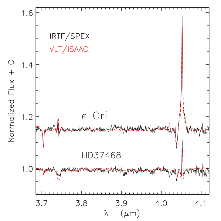
Figure 2: Comparison between IRTF/SpeX (solid) and VLT/ISAAC (dashed) $L$-band spectra for the two objects (HD 37468 and $\epsilon$ Ori) observed in both runs. The VLT/ISAAC spectra have been reduced to the resolution of the IRTF/SpeX instrument. Note the excellent agreement between both datasets.

The validity of the reduction procedure for each dataset is confirmed in Fig. 2, where a comparison between IRTF/SpeX and VLT/ISAAC $L$-band spectra for the two objects (HD 37468 and $\epsilon$ Ori) observed in both runs is presented. In Fig. 2 the VLT/ISAAC spectra have been reduced to the resolution of the IRTF/SpeX instrument (note the larger S/N ratio of the former). The excellent agreement between both datasets clearly supports the different data reduction procedures employed for each run. Given the higher resolution of the VLT/ISAAC data, we made use of these observations for our quantitative analysis.

3 IR diagnostics

To model the infrared spectra of our sample of objects we have utilized cmfgen, which is an iterative, non-LTE, line-blanketed model atmosphere/spectrum synthesis code developed by Hillier & Miller (1998). It solves the radiative transfer equation in the co-moving frame and in spherical geometry for the expanding atmospheres of early-type stars. The model is prescribed by the stellar radius, $R_{\ast}$, the stellar luminosity, $L_{\ast}$, the mass-loss rate, ${\dot{M}}$, the velocity field, $v(r)$ (defined by $v_{\rm\infty}$ and $\beta$), the volume filling factor characterizing the clumping of the stellar wind, and elemental abundances. Following Hillier & Miller (1998, see also ) we include X-rays characterizing the X-ray emissivity in the wind by two different shock temperatures, velocities and filling factors. We refer to Hillier & Miller (1998, 1999) for a detailed discussion of the code.

Table 2: Stellar and wind parameters as adopted/derived in the present analysis. $T_{\rm eff}$ in kK, $R_{\ast}$ in $\rm{R_{\odot}}$, all velocities in km s^-1, ${\dot{M}}$ in $10^{-6}\,{\rm M_{\odot}/yr}$ and modified wind-momentum rate, $D_{\rm mom}=\dot{M}v_{\infty}(R_{\star}/R_{\odot})^{0.5}$, in cgs. The gravitational acceleration, $\log g$, is the effective one, i.e., not corrected for centrifugal forces. The volume filling factor, $f_{\rm v}$, corresponds to the parameter CL₁ in Eq. 1 and describes the maximum degree of clumping reached in the stellar wind. However, since our analysis bases on stratified clumping factors, the usual scaling of $\dot{M}\propto\sqrt{f_{\rm v}}$ does not or only approximately apply in most cases. CL₂ (km s^-1) indicates the onset of clumping in the wind. The horizontal line separates objects displaying significant wind emission in H_α, i.e., dense winds (see Sect. 4), from objects with a pure absorption H_α profile, i.e., thin winds (Sect. 5).

star	sp.type	Mv	$T_{\rm eff}$	$\log g$	$R_{\ast}$	$Y_{\rm He}$	$\log(L/L_{\odot})$	$v\sin i$	$v_{\rm macro}$	$v_{\rm\infty}$	${\dot{M}}$	$\beta$	$f_{\rm v}$	CL2	$v_{\rm{turb}}$	$\log D_{\rm mom}$
Cyg OB2 $\#$7	O3 If∗	-5.911	45.1	3.75	14.7	0.13	5.91	95	65	3100	1.2	1.05	0.03	100	10	28.95
HD 66811	O4 I(n)f	-6.322	40.0	3.63	18.9	0.14	5.92	215	95	2250	2.1	0.90	0.03	180	10	29.11
Cyg OB2 $\#$8C	O5 If	-5.611	37.4	3.61	14.3	0.10	5.56	175	90	2800	2.0	1.30	0.10	550	20	29.13
Cyg OB2 $\#$8A	O5.5 I(f)	-6.911	37.6	3.52	26.9	0.10	6.12	110	80	2700	3.4	1.10	0.01	500	10	29.48
HD 30614	O9.5 Ia	-7.002	28.9	3.01	32.0	0.13	5.81	100	75	1550	0.50	1.60	0.01	25	17.5	28.44
HD 37128	B0 Ia	-6.993	26.3	2.90	34.1	0.13	5.70	55	60	1820	0.46	1.60	0.03	30	15	28.49
HD 217086	O7 Vn	-4.502	36.8	3.83	8.56	0.1	5.08	350	80	2510	0.028	1.2	0.10	30	10	27.11
HD 36861	O8 III((f))	-5.394	34.5	3.70	13.5	0.11	5.37	45	80	2175	0.28	1.3	1.0	-	7.5	28.15
HD 76341	O9 Ib	-6.294	32.2	3.66	21.2	0.1	5.64	63	80	1520	0.065	1.2	1.0	-	7.5	27.46
HD 37468	O9.5 V	-3.904	32.6	4.19	7.1	0.1	4.71	35	100	1500	0.0002	0.8	1.0	-	5	24.70

¹ Mokiem et al. (2005), ² Repolust et al. (2004), ³ Kudritzki et al. (1999), ⁴ from the calibration provided by Martins et al. (2005a).

Given the large range of stellar parameters and the variety of luminosity classes covered by our O-star sample, the location of the $\tau_{\rm Ross}=2/3$ radius for these objects will vary from being placed in the deep hydrostatic layers (dwarfs) up to the upper layers where the wind takes off (supergiants). Noting that not only the IR lines but also the IR continuum, through bound-free and free-free processes, will have different formation depths as a function of wavelength, the role of the hydrostatic structure and the transition region between photosphere and wind becomes crucial to interpret the stellar spectra.

With this in mind, we computed CMFGEN models with a photospheric structure modified following the approach from Santolaya-Rey et al. (1997) , smoothly connected to a beta velocity law. In our approach the Rosseland mean from the original formulation was replaced by the more appropriate flux-weighted mean. Several comparisons using “exact” photospheric structures from tlusty (Hubeny & Lanz 1995) showed excellent agreement with our method. Likewise, model atoms were expanded and optimized to make use of the IR metal lines arising from high lying levels.

To investigate the role of clumping, we follow the conventional approach of microclumping and assuming a void inter-clump matter. In this case, and as already outlined in Sect. 1, the volume filling factor is just the inverse of the clumping factor, $f_{\rm v}=f_{\rm cl}^{-1}$, and the clumping factor itself quantifies the overdensity of the clumps with respect to the averaged density, $\langle\rho\rangle=\dot{M}/(4\pi r^{2}v(r))$. Moreover, the radial stratification of the volume filling factor is described by the clumping law introduced by Najarro et al. (2009):

$$f_{\rm v}(r)=CL_{1}+(1-CL_{1})\,{\rm e}^{-\frac{v(r)}{CL_{2}}}+(CL_{4}-CL_{1})\,{\rm e}^{-\frac{v_{\infty}-v(r)}{CL_{3}}}$$ (1)

where CL₁ and CL₄ are volume filling factors and CL₂ and CL₃ are velocity terms defining locations in the stellar wind where the clumping structure changes. CL₁ sets the maximum degree of clumping reached in the stellar wind (provided CL₄ $>$ CL₁) while CL₂ determines the velocity of the onset of clumping. CL₃ and CL₄ control the clumping structure in the outer wind. From Eq.1 we note that as the wind velocity approaches $v_{\rm\infty}$, so that $(v_{\infty}-v(r))\leq$ CL₃, clumping starts to migrate from CL₁ towards CL₄. If CL₄ is set to unity, the wind will be unclumped in the outermost region. Such behavior was already suggested by Nugis et al. (1998) and was utilized by Figer et al. (2002) and Najarro et al. (2004) for the analysis of the WNL stars in the Arches Cluster. Recently, Puls et al. (2006) have found a similar behavior from H_α and IR/mm/radio studies for OB stars with dense winds. Furthermore, our clumping parametrization seems to follow well the results from hydrodynamical calculations by Runacres & Owocki (2002). From Eq. 1 we note that if the term including CL₃ and CL₄ is neglected or if CL${}_{3}\rightarrow$ 0, we recover the law proposed by Hillier & Miller (1999). For the present study (except for $\zeta$ Pup, see below), we have set CL₄=1, i.e., the outer wind regions are assumed to be unclumped.

Observational constraints are set by the $L$-band spectra presented above and UV, high-resolution optical and $H$ and $K$-band spectra collected by our group as well as by optical, IR and radio continuum measurements from literature/archival data. The individual sources are quoted in the corresponding figure captions. In this paper we concentrate on the strong diagnostic potential provided by the infrared $K$- and $L$-bands to determine mass-loss rates and trace wind clumping as an alternative to H_α, the classical mass loss indicator. Thus, we defer a detailed full wavelength analysis and discussion of these objects to a forthcoming paper.

Table 2 displays the stellar parameters obtained for our sample, whereas a detailed comparison with results from previous investigations is provided in Appendix A. We obtain uncertainties of $\sim$1000 K for the effective temperature of the objects (see Appendix A for a thorough discussion) while typical errors of 0.1 dex are estimated for $\log g$. For objects with dense wind, we estimate our mass-loss accuracy to be better than 25%, with the corresponding ${\dot{M}}$/$f_{\rm v}^{0.5}$ = const scaling for the error on the clumping factor. For objects with thin winds we consider 0.5 dex as a conservative error on the mass-loss rate estimate (see Sect. 6.1).

Projected rotational speeds, $v\sin i$, have been derived via the Fourier-transform technique as developed by Simón-Díaz et al. (2006) (based on the original method proposed by Gray 1973, 1975), applied to weak metal lines (and partly Hei-lines) available in the spectra. The remaining discrepancies between synthetic and observed lines were “cured” by convolving the spectra with an additional, radial-tangential macro-turbulent velocity distribution (entry $v_{\rm macro}$ in Table 2). The derived values are of similar order as found in alternative investigations (Ryans et al. 2002, Simón-Díaz et al. 2006, Simón-Díaz & Herrero 2007, Lefever et al. 2007, Markova & Puls 2008), indicating highly supersonic speeds in photospheric regions that would be difficult to explain. Recently, however, Aerts et al. (2009, see also ) interpreted such extra-broadening in terms of collective effects from hundreds of non-radial gravity-mode oscillations, where the individual amplitudes remain sub-sonic. They pointed out that the rotational velocity could be seriously underestimated whenever the line profiles are fitted assuming a macroturbulent velocity rather than an appropriate expression for the pulsational velocities, or if a Fourier technique is applied to infer the rotational velocity. If this were true, our values for $v\sin i$ (and also those from the quoted investigations) would provide only lower limits. For the present investigation, however, this is of minor concern, since our main interest is to obtain a correct shape of the profiles (irrespective of the responsible process), to enable meaningful fits.

4 Objects with dense winds, constraints on the clumping factor

In this section we discuss our results for the objects of our sample displaying dense winds, and compare them with previous studies carried out at optical (Repolust et al. 2004, hereafter REP04; Mokiem et al. 2005, MOK05) and near-infrared wavelengths (Repolust et al. 2005, REP05) as well as the combined H_α/IR/mm/radio analysis by Puls et al. (2006, hereafter PUL06). For further details, see Appendix A.

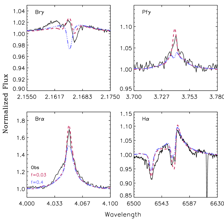
Figure 3: Model fits to IR and H_α observations of Cyg OB2 #7 (solid, black). Two different models corresponding to clumping values of $f_{\rm v}$=0.03 (dashed, red) and $f_{\rm v}$=0.4 (dashed-dotted, blue) are displayed (see text). The H_α spectrum was obtained with ISIS at the William Herschel Telescope on La Palma (kindly provided by A. Herrero).

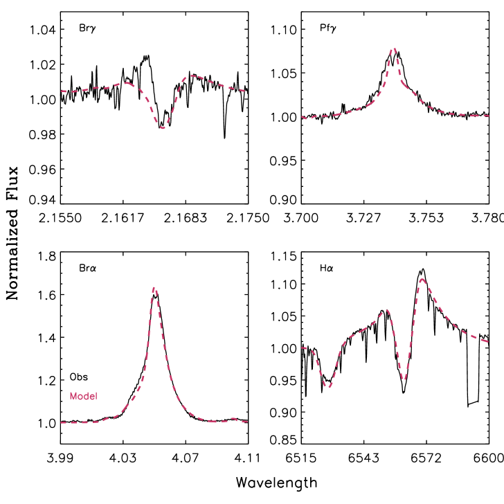
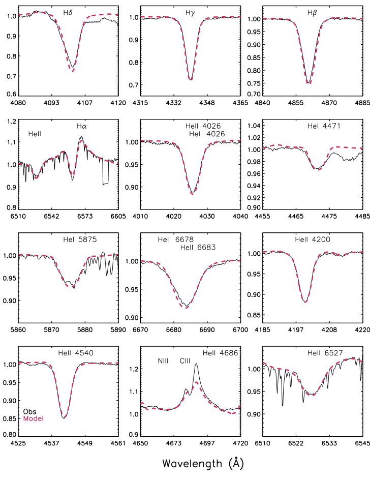
Figure 4: Model fits (dashed) to IR and optical observations of $\zeta$ Pup (solid). Optical data were retrieved from the ESO archive, programme 266.D-5655(A)

Cyg OB2 #7.

Our derived main stellar parameters for Cyg OB2 #7 (see Table 2) agree very well with those obtained from optical (MOK05) and $H$ and $K$-band (REP05) analyses with respect to the effective temperatures (within less than 1000 K). This is a very encouraging result since our temperature determination relies not only on the Heii/Hei equilibrium (e.g., , ) but also on the Nv/Niv/Niii equilibria. Our results confirm the consistency between both criteria and the validity of the weak Hei lines as diagnostics in this high temperature regime. Likewise, our $\log g$ value lies in between the ones derived by MOK05 and REP05, while our unclumped mass-loss rates ($\sim$ 7.8 $\cdot 10^{-6}\,{\rm M_{\odot}/yr}$) are roughly 30% lower. We attribute this discrepancy to our lower He abundance (0.13 vs 0.21 in MOK05) and higher $\beta$ (1.0 vs 0.8). Interestingly, our models favor a large clumping starting relatively close to the photosphere to provide consistent simultaneous fits to the UV, optical and IR observations of this object (see Fig. 3). However, such a strong clumping – via the corresponding lower mass-loss rate – tends to produce much too deep cores in the optical H and Heii lines. For comparison, a less clumped model ($f_{\rm v}$=0.4), better matching the optical lines, is also displayed in Fig. 3. Note, however, that such a model leads to severe mismatches with the $L$-band and UV (not displayed here) spectra. From Fig. 3 we see that in the case of strong winds Br_γ and Pf_γ provide stronger response to clumping than Br_α. PUL06 also found a strong clumping in the inner wind of this object. Their average clumping factors lie between the ones we obtain in our IR and optical analysis. We would like to stress that while the optical and IR spectra of Cyg OB2 #7 provide strong constraints on CL₁ and CL₂, the UV spectra and submillimeter and radio observations constitute crucial diagnostics to determine CL₄ and CL₃. Indeed, our UV and submillimeter data (Najarro et al. 2008) support the presence of constant clumping, at least up to mid-outer wind regions where the millimeter continua of Cyg OB2 #7 are formed. However, radio observations by PUL06 show that clumping may start to vanish at the outermost regions of the stellar wind (note that radio continua form at much larger radii). The expected emission of our models with constant clumping severely overestimate the upper limits provided by the observations by PUL06 of Cyg OB2 #7. This demonstrates the need of multiwavelength observations to constrain the run of the clumping structure.

$\zeta$ Puppis.

Our derived main stellar parameters agree fairly well with those presented by REP04 and REP05. We find, however, a slightly lower He abundance and a much higher (by 50%) “unclumped” mass-loss rate. We attribute this discrepancy in ${\dot{M}}$ to our clumping parametrization for this object. Given the large number of spectroscopic and continuum constraints at nearly all wavelengths available for $\zeta$ Pup, we performed a detailed clumping study aiming to constrain as accurately as possible the run of the clumping factor throughout the wind and compare it with recent results from PUL06. Thus, we made use of all the clumping parameters presented in Eq.1 and obtained CL₁=0.03, CL₂=180., CL₃=600 and CL₄=0.17 as a best fit (see Fig. 18). With this parametrization, maximum clumping ($f_{\rm v}$=0.03) is reached only in a very narrow, $\Delta R\approx 0.1$ $R_{\ast}$, region around r=1.5 $R_{\ast}$. Thus, the classical ${\dot{M}}$/$f_{\rm v}^{0.5}$ = const scaling for constant clumping does not hold and causes the above discrepancy regarding unclumped ${\dot{M}}$ values. Our best model (see Fig.4) is able to reproduce satisfactorily not only the $L$- and $K$-band spectra but also the optical lines and the full UV to radio energy distribution of the object. We stress the almost perfect fit reached for H_α. That quality of fit can only be achieved for models with stratified clumping as otherwise the observed absorption and emission components cannot be fitted simultaneously (see also PUL06). We note, however, that since we aimed at a compromise solution, our model is unable to fit the blue wing of Br_γ. Thus, while a different clumping would yield a better fit to Br_γ, it would also worsen significantly the model fits to other lines.

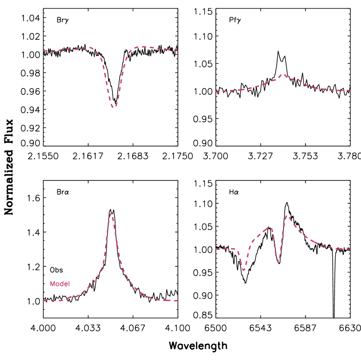
Figure 5: Model fits (dashed) to IR and H_α observations of Cyg OB2 #8C (solid). H_α observations as in Fig. 3.

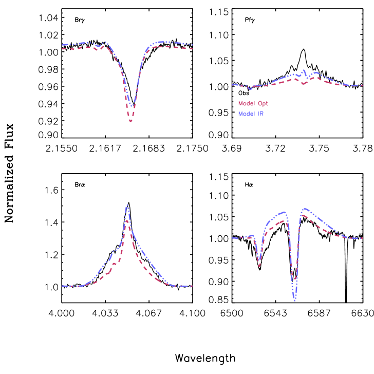
Figure 6: Model fits to IR and H_α observations of Cyg OB2 #8A. (solid, black). Best model fitting only the optical (dashed, red) is displayed together with that providing the best fit to the IR data (dashed-dotted, blue) (see text). H_α observations as in Fig. 3.

In their analysis of the clumping structure of O-star winds, PUL06 pointed out that the derived clumping values for $\zeta$ Pup are strongly dependent on the assumptions regarding the run of the He ionization. Interestingly, their maximum clumping factors ($\sim$5 for Heiii recombining at v=0.86$v_{\rm\infty}$and $\sim$11 for a wind with completely ionized He, when assuming an unclumped outer wind) are reached in the same wind region (i.e. around r=1.5 $R_{\ast}$) as in our models. When scaled to a similar outer clumping factor as derived in this work, the agreement is even more striking (see Fig. 18). Thus, both studies reach the same conclusions concerning the run of the clumping factor. As for Cyg OB2 #7, our investigation shows the high sensitivity of Br_γ and Pf_γ to clumping (see Fig. 4) and the enormous potential of IR spectroscopy to constrain the structure of stellar winds.

Cyg OB2 #8C.

The derived stellar parameters differ considerably from those obtained by MOK05. Our temperature is more than 4000 K lower while our gravity lies only 0.12 dex below. We are confident in our temperature determination since, as discussed above, we make use of both helium and nitrogen ionization equilibria (see Fig.5). In fact, our model reproduces satisfactorily the optical and IR spectra of this object. We suggest that the discrepancy is closely related to the lower $v\sin i$ derived by MOK05 ($v\sin i$=145 km s^-1vs. our 175 km s^-1+ 90 km s^-1macroturbulence) and the strong reaction of Hei 4471 in this parameter domain. The difference in derived $v\sin i$ values can be attributed to the fact that our spectra are of higher quality than those used by MOK05. We stress that our best compromise solution underestimates the emission core of Pf_γ.

Compared to the other strong wind objects discussed in this section, this object requires a lesser degree of clumping. Further, our models imply an onset of clumping which is located at larger velocities than for the rest of our supergiants. PUL06 also derived a low degree of clumping. However, a detailed comparison with their results is not possible as their analysis of this object remained rather unconstrained due to the lack of sufficient flux measurements.

Cyg OB2 #8A.

Unlike for the case of Cyg OB2 #8C, our analysis of Cyg OB2 #8A yields excellent agreement with the stellar parameters obtained by MOK05. de Becker et al. (2004) report this object to be a O6I + O5.5III binary system. This can be clearly inferred from the absolute magnitude of the system displayed in Table2. In fact, no single best fit could be obtained to fit simultaneously the optical and IR observations of Cyg OB2 #8A (see Fig.6). Our preferred model, which reproduces better the IR spectra, is characterized by strong clumping ($f_{\rm v}$=0.01) that leads, as in the aforementioned case of Cyg OB2 #7, to somewhat too strong absorption cores in the optical hydrogen lines. We note that the inclusion of clumping nicely removes the discrepancy in Br_γ found by REP05. On the other hand, a model with $f_{\rm v}$=0.1 tuned to optimize the optical (see Fig.6) severely underestimates the emission components in the IR lines. The analysis of PUL06 was hindered by the non-thermal nature of Cyg OB2 #8A’s radio emission. Nevertheless, their combined H_α + IR photometry analysis yields a wind structure which is significantly less clumped than inferred in this paper. Both results could be only reconciled if the outer wind would be strongly clumped.

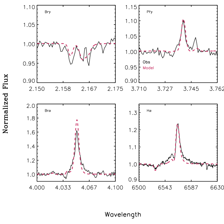
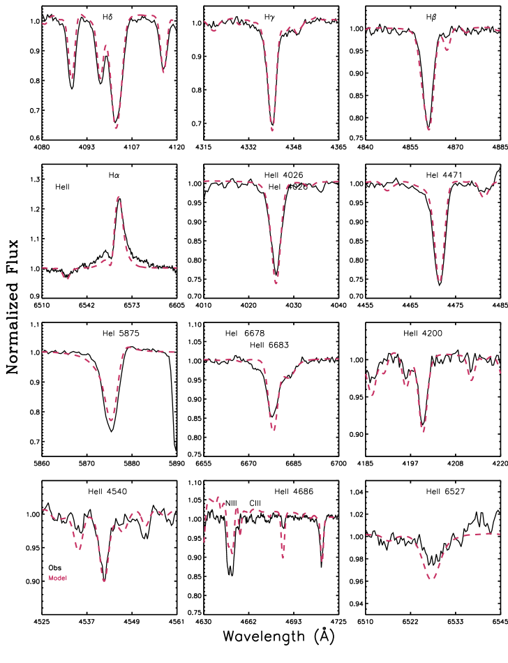
Figure 7: Model fits (dashed) to IR and optical observations of $\alpha$ Cam (solid). Optical data are from the Indo-U.S. Library of Coudé Feed Stellar Spectra (Valdes et al. 2004).

$\alpha$ Cam.

We find excellent agreement with the stellar parameters derived by REP05. A very high degree of clumping, starting very close to the photosphere, is required to match Pf_γ. In fact, this line turns into the most sensitive clumping diagnostic at the base of the wind in O supergiants. Our result agrees qualitatively with PUL06’s conclusions on the run of the clumping factor. They found a moderate degree of clumping in the inner and mid wind regions. Figure 7 shows that our model can reproduce satisfactorily the IR and optical spectra of HD 30614.

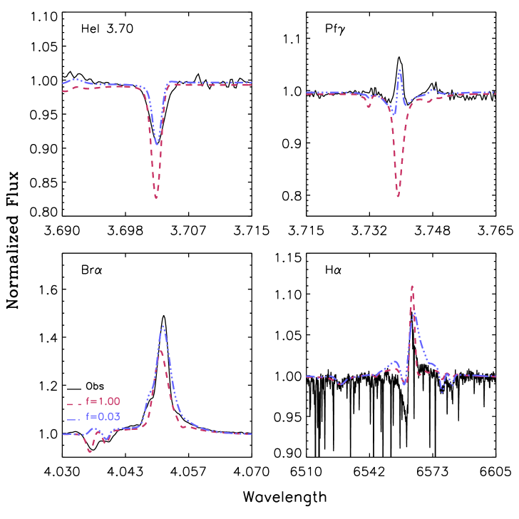
Figure 8: Model fits to IR and H_α observations of $\epsilon$ Ori (solid, black). Two different models corresponding to no clumping (dashed, red) and a clumping value $f_{\rm v}$=0.03 (dashed-dotted, blue) are displayed (see text). The H_α profile was kindly provided by N. Przybilla.

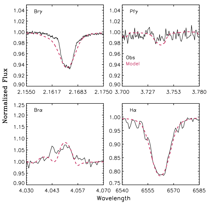
Figure 9: Model fits (dashed) to IR and H_α observations of HD 217086 (solid). H_α observations as in Fig.3.

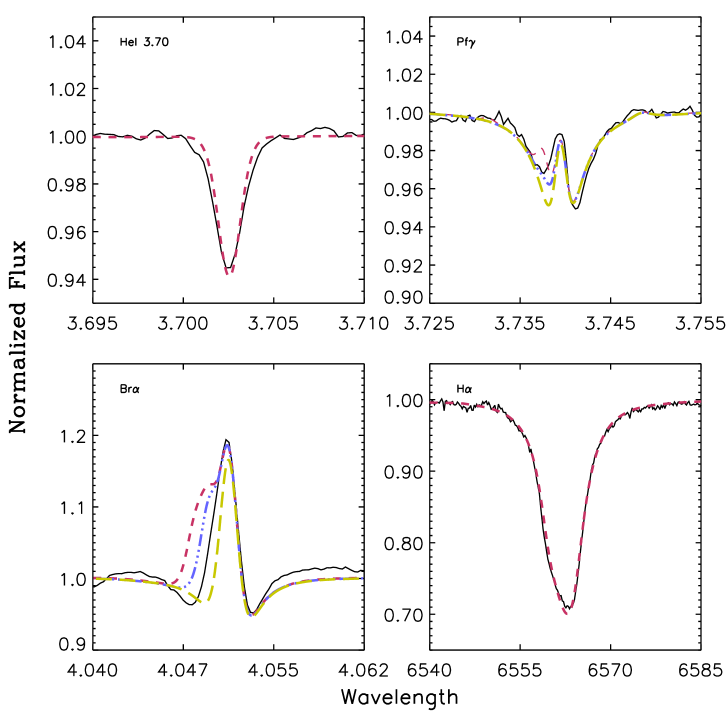
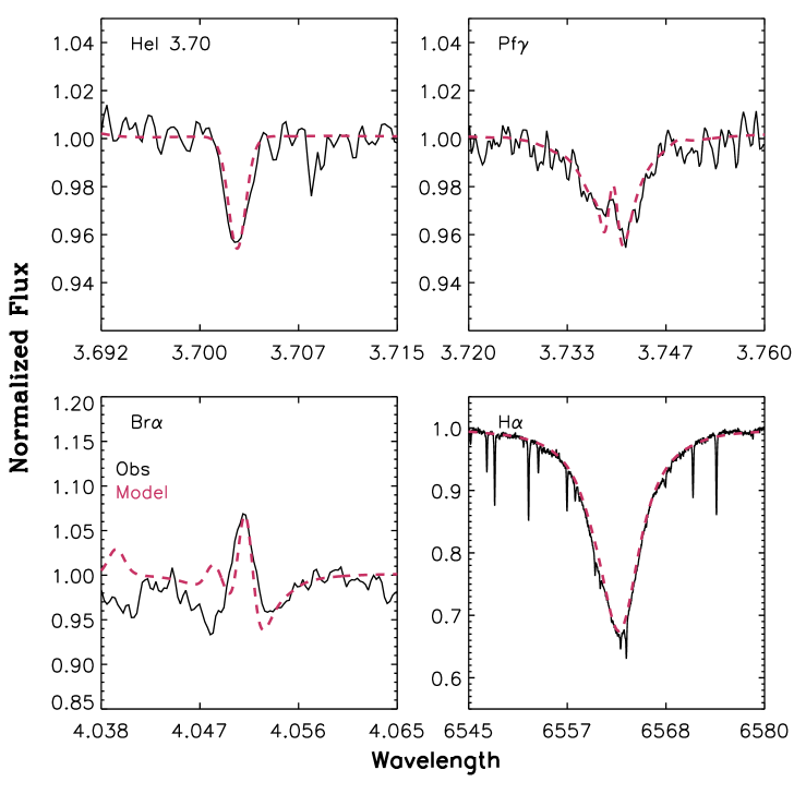
Figure 10: Model fits (dashed) to IR and optical observations (solid) of HD 36861 (top) and HD 76341 (bottom). For HD36861 we show as well model fits to Pf_γ and Br_α computed without Hei components (dashed-dotted), and with no He at all (long dashed, see text). Optical data were retrieved from the UVES POPS Catalog archive, programme 266.D-5655(A).

$\epsilon$ Ori.

Several spectroscopic studies of $\epsilon$ Ori using cmfgen (e.g. Searle et al. 2008) and fastwind (REP05), yielding similar parameters, have recently appeared in the literature. While the cmfgen study made use of UV and optical data, the fastwind one used infrared spectroscopic observations alone. Interestingly, REP05 could derive only an upper limit on the effective temperature due to the absence of Heii IR diagnostic lines. Our results, arising from a full UV to IR investigation and displayed in Table2, revise down the effective temperature by roughly 1000 K. A striking result revealed by Fig.8 is the requirement of strong clumping to match the IR spectra. Figure 8 demonstrates the failure of an unclumped ($f_{\rm v}=1$) wind to reproduce the $L$-band lines. As for most of the previous stars, such strong clumping leads to overestimated HI and Hei line cores. In the case of $\epsilon$ Ori, however, this mismatch could be also due to the intrinsic line profile variability, as the IR and optical observations where taken at different epochs.

5 Objects with thin winds

HD 217086.

Our derived stellar parameters for this fast rotating dwarf are in excellent agreement with those obtained by REP04 and REP05 by means of optical and IR spectroscopy. While their IR analysis could provide an upper limit to the mass-loss rate being a factor of two lower than the optical one, no firm determination of this parameter could be assessed. Our $L$-band data (see Fig. 9) clearly show how Br_α constitutes a much more powerful ${\dot{M}}$ diagnostic for low density winds than the previously used H_α and Br_γ lines. Our UV through IR study yields a less clumped wind than for the case of the supergiants. Without the UV we could not have broken the ${\dot{M}}$- clumping degeneracy though.

HD 36861.

This object displays the strongest wind within our sample of stars with low density winds, as to be expected from its O8 III((f)) spectral type classification. Our derived effective temperature is hotter than the one adopted by PUL06 (based on the calibrations used by Markova et al. 2004). Interestingly, no clumping is required by our models to match the IR and optical lines. This result is consistent with one of the two possible solutions found by PUL06. Figure. 10 (upper two panels) shows the excellent agreement of our models with the observations. Exceptions are two of the optical Hei singlets (related to the so-called singlet problem, Najarro et al. 2006) and the He components of the IR H lines. Our models (see Fig. 10, upper left) tend to show the Hei components in emission. Since this discrepancy appears only in objects with low density winds where the Hei hydrogenic components form at higher densities, we suggest that realistic broadening functions should be developed and used to replace the assumed pure Doppler profiles.

HD 76341.

As for HD 36861, no clumping is required to reproduce optical and IR (also UV, not shown here) spectra of HD 76341 (Figure 10, lower two panels). Again we note the problem with the Hei components in Br_α, but also the enormous potential of this line to determine mass-loss rate in thin winds when H_α struggles to react to changes in ${\dot{M}}$.

Figure 11: Model fits (dashed) to IR and H_α observations of HD 37468 (solid). The H_α profile was obtained with IDS at the INT Telescope on La Palma (kindly provided by S. Simón-Díaz).

HD 37468.

This is the object with the thinnest wind in our sample. Our analysis has made use of available UV and optical spectra as well. Once more, no clumping is required and we obtain ${\dot{M}}$= 2 $\cdot 10^{-10}\,{\rm M_{\odot}/yr}$ as our current best estimate (see Fig. 11). The need of correct broadening functions for the Hei lines is again evident in the Br_α complex. Even though our ${\dot{M}}$ determination appears perfect, we stress that in this regime of extremely low mass-loss rates the resulting synthetic Br_α profile can be very sensitive to the data set used for the hydrogen collisional bound-bound processes (see below).

In the following, we will discuss the formation of the specific shape of the Br_α profile in these very thin winds in considerable detail.

5.1 Theoretical considerations

As has been extensively discussed by Mihalas (1978), Kudritzki (1979), Najarro et al. (1998), Przybilla & Butler (2004) and Lenorzer et al. (2004), the low value of $h\nu/kT$ in the IR leads to the fact that even small departures from LTE become substantially amplified (in contrast to the situation in the UV and optical). This can be immediately seen from the line source-function in the Rayleigh-Jeans limit,

$$S_{L}/B_{\nu}\approx(1+\delta/(h\nu/kT))^{-1},\qquad\delta=b_{l}/b_{u}-1$$ (2)

where $b_{l}$ and $b_{u}$ are the NLTE departure coefficients for the lower and upper level, respectively. For temperatures at 30 kK, the value of $h\nu/kT$ is 0.24 at Br_γ and 0.11 at Br_α. Thus, under typical thin-wind conditions (where in the line forming region the lower level becomes underpopulated compared to the upper one, see below) the line source-function can easily exceed the continuum, or can become even “negative”, i.e., dominated by induced emission. E.g., for the case of $b_{l}/b_{u}=0.95$, $S_{L}/B_{\nu}\approx 1.83$ at Br_α, whereas for a ratio of 0.9 already a value of $S_{L}/B_{\nu}\approx 11$ is present, and lasering sets in at a ratio of 0.89.

From these examples, it is immediately clear that the synthesized profile, particularly Br_α, reacts very sensitively to this ratio, where the major effect regards the height of the narrow emission peak that we will use to constrain the mass-loss rate. Thus, we must also check the influence of uncertainties in atomic data and atmospheric parameters that can influence this ratio and might weaken our conclusions.

To investigate the general formation mechanism and the above problems, we have calculated a large number of models exploring the sensitivity of Br_α on various effects, and will comment on those in the following, by means of our model of HD 37468 with atmospheric parameters as outlined in Table 2.

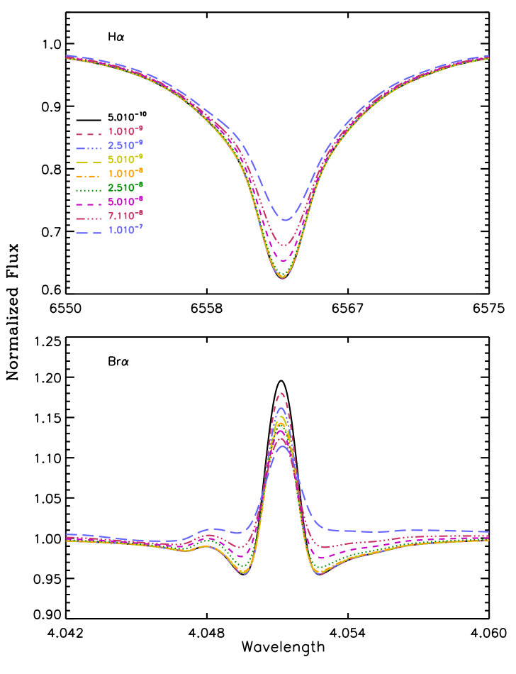
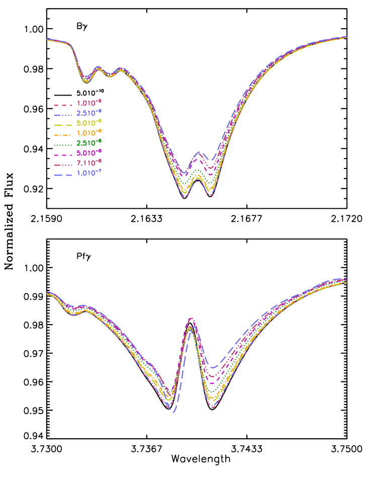
Figure 12: H_α, Br_α, Br_γ, and Pf_γ  profiles for our model of HD 37468 and different mass-loss rates (see text).

General behavior.

In Fig. 12, we compare the reaction of H_α, Br_α, Br_γ, and Pf_γ on different mass-loss rates, varied within ${\dot{M}}$ = 5$\cdot 10^{-10}$ (solid black) and 1$\cdot 10^{-7}\,{\rm M_{\odot}/yr}$ (long-dashed, blue). Whereas a clear reaction of H_α is found only for ${\dot{M}}$ $\geq$ 5$\cdot 10^{-8}\,{\rm M_{\odot}/yr}$, Br_α remains sensitive at even the lowermost values. For increasing mass-loss, the height of the emission peak in Br_α decreases, whereas the wings (in absorption for lowest ${\dot{M}}$) become more and more refilled, going into emission around $10^{-7}\,{\rm M_{\odot}/yr}$. From Fig. 12 we note that also the Br_γ and Pf_γ line profiles are more sensitive than H_α in the thin wind regime as their wings typically require a factor of 5 lower ${\dot{M}}$ to start displaying reactions to mass-loss.

The refilling of the wings with increasing mass-loss can be explained by the increasing influence of the bound-free and free-free continuum (i.e., the typical continuum excess in stellar winds becomes visible) as well as a certain “conventional” wind emission. However, at line center the line processes always dominate and the peak height depends on the location (in $\tau$) where the wind sets in. This is shown in Fig. 13 which relates the strength of the Br_α source function at each point of the atmosphere with the gradient of velocity field and reveals whether the photosphere, transition region or wind control the resulting Br_α line profile.

Depopulation of the $n=4$ level in the outer photosphere.

As outlined in the introduction, already Auer & Mihalas (1969) found in one of their first NLTE-models a stronger depopulation of $n=4$, compared to $n=5$. They argued as follows: Whenever the density becomes so low that collisional coupling plays no role, the decisive processes are recombination and cascading, as in nebulae. Because the decay channel 4 $\rightarrow$ 3 is very efficient in this process, level 4 becomes stronger depopulated than level 5, and the core of Br_α goes into emission.

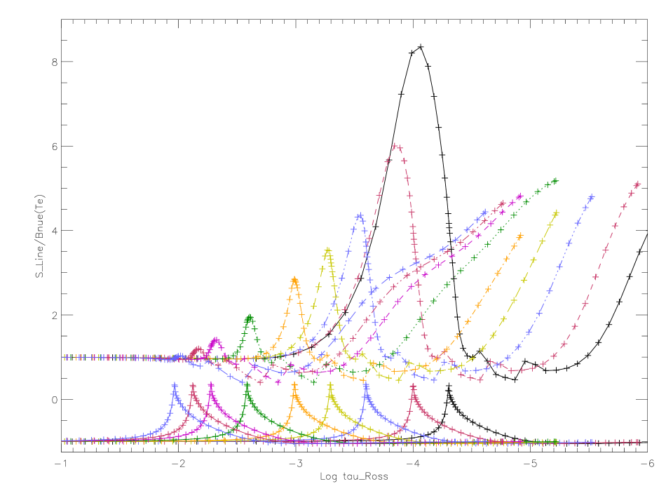
Figure 13: Line source function of Br_α (in units of the local Planck function) and velocity gradient (vertically scaled) as a function of $\tau_{\rm Ross}$, for the same ${\dot{M}}$-sequence as in Fig. 12. Note that the transition region between photosphere and wind moves towards lower $\tau_{\rm Ross}$ for decreasing ${\dot{M}}$, i.e., the model with the lowest mass-loss is located at the right of the figure.

Since their findings refer to different conditions ($T_{\rm eff}$ = 15,000 K), and since it is important to understand the dependence of the depopulation on the precision of the involved processes, we investigated the process in more detail. As it turned out that line-blocking/blanketing effects have a minor influence on the principal results for hydrogen (only the absolute peak height of Br_α is affected, but not its systematic behavior), we used a pure hydrogen/helium model (with parameters as derived for HD 37468, but with a very weak wind, ${\dot{M}}$= $5\cdot 10^{-12}$ ${\rm M}_{\odot}$/yr) for this purpose, in order to allow for a multitude of calculations. The results of our investigation are displayed in Fig. 14. In the optically thin part of the photosphere ($10^{-4}<\tau_{\rm Ross}<10^{-8}$), all departures remain roughly constant, where the ground-state (dashed-dotted) is overpopulated by a factor of 10, the 2nd level (solid) is roughly at LTE and, indeed, $b_{4}$ (dashed) is smaller than $b_{5}$ (dotted). In contrast, the groundstate is strongly overpopulated in the wind ($\propto r^{2}$ for constant temperature, see below), whereas the excited levels are overpopulated by factors between 10 and 5, with a different order than in the photosphere, i.e., $b_{5}<b_{4}<b_{2}$.

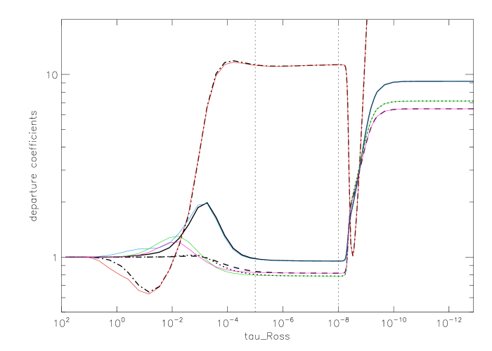
Figure 14: Underpopulation of the hydrogen $n=4$ level (compared to $n=5$) in the outer photospheres of late-type O-dwarfs with very thin winds (pure H/He model atmosphere).
Left: Departure coefficients for $n=1,2,4,5$ (dashed-dotted, solid, dotted, dashed), accounting for all processes (radiative and collisional). Overplotted are the corresponding departure coefficients (red, blue, green, magenta) as resulting from a NLTE solution discarding the collisional processes. Note the underpopulation of $n=4$ compared to $n=5$ in the outer photosphere (responsible for the line core emission in Br_α), which is no longer present in the wind.
Right: Departure coefficients of $n=2,4,5$ (solid, dotted, dashed) in the outermost photosphere (corresponding to the region embraced by dotted lines on the left), as resulting from the complete NLTE solution and various approximations, the latter all without collisions: 2: nebula approximation (Case A); 3: as 2, but including excitation/induced deexcitation from resonance lines (roughly Case B); 4: as 3, but including ionization from excited states; 5: as 4, but including excitation/deexcitation from all lines with lower level $n\leq 3$; 6: as 4, but including excitation/deexcitation from all lines with lower level $n\leq 5$ (see text).

In the following, we will investigate the influence of various effects that determine this pattern, by solving the NLTE rate equations and omitting certain rates, but using a fixed radiation field (which is legitimate at least in the optically thin part of the atmosphere).

At first, we checked the influence of the collisional rates, by leaving them out everywhere. The result of this simulation is displayed on the left of Fig. 14. Obviously, below $\log\tau_{\rm Ross}=-5$ collisions do not play any role, since the departure coefficients with (in black) and without (in color) collisions are identical. In the lower photosphere, of course all departures are affected by collisions, but particularly for level 4 and 5 a difference is visible until $\log\tau_{\rm Ross}=-5$, where these levels remain thermalized until $\log\tau_{\rm Ross}=-2$. Since the major part of the line core forming region of Br_α is just in the range between $10^{-2}<\tau_{\rm Ross}<10^{-4}$, we have to conclude that collisions do play a certain role in the formation of Br_α, and will return to this point later on.

Before doing so, however, we try to understand the depopulating processes in the outer photosphere (opposed to the conditions in the wind) by concentrating on that part which is not affected by collisions, in order to gain insight into the dominating mechanism. To this end, we display the results of various approximations on the right of Fig. 14, by considering the outermost photosphere (indicated by dotted lines on the left panel).

The first approximation (“2”) follows the suggestion by Auer & Mihalas (1969), i.e., we solved the rate-equations for a Case A nebula approximation, i.e., allowed for ground-state ionization, spontaneous decays and radiative recombination into the excited levels. In this case, we derive departures with $1>b_{5}>b_{4}>b_{2}$ (i.e., level 4 is more strongly depopulated than level 5), but far away from the complete solution. Moreover, the ground-state (not displayed) is roughly consistent with the exact solution, whereas the departures of the excited levels in the wind do not differ from the conditions in the outer photosphere.

In simulation 3, we switched on the resonance lines, by including the corresponding excitation and induced deexcitation rates (roughly corresponding to Case B nebula conditions). Immediately, all departures in the wind obtain values very close to the complete model (i.e., $b_{2}>b_{4}>b_{5}>1$), whereas in the outer photosphere the “correct” order is achieved ($b_{2}>b_{5}>b_{4}$), though at a much too high level.

This is cured by simulation 4, where ionization from the excited states is switched on. By this process, all levels are depopulated again, and the corresponding solution looks very close to the exact one. (The departures in the wind remain unaffected, since these rates are almost unimportant because of the strongly diluted radiation field).

One might conclude now that the remaining missing rates (excitation/deexcitation between excited levels) are negligible. Unfortunately, this is not the case, at least if one is interested in the precise ratio of $b_{5}/b_{4}$, which is of major importance in our investigation. Though the line transitions between the excited states are optically thin, the mean line intensity is still large enough to be of influence. This becomes clear by comparing simulation 5 with 6. In the former, we have included the excitation/deexcitation from all lines with lower level $n\leq 3$ (i.e., level 4 and 5 are only affected by line transitions in terms of resonance lines and spontaneous decay), with the effect that now $b_{4}\ga b_{5}$, i.e., the emission core of Br_α would disappear. Only if all bound-bound processes for lines with at least a lower level of $n\leq 5$ are included (simulation 6), the “exact result” is recovered (i.e., higher levels contribute indeed almost only by spontaneous decay).

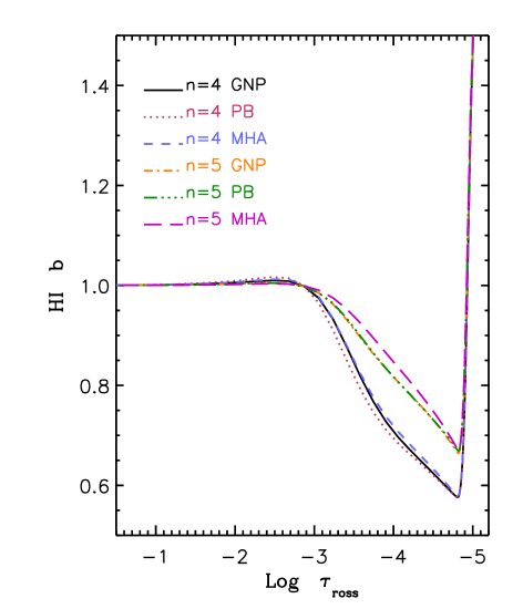
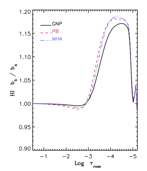
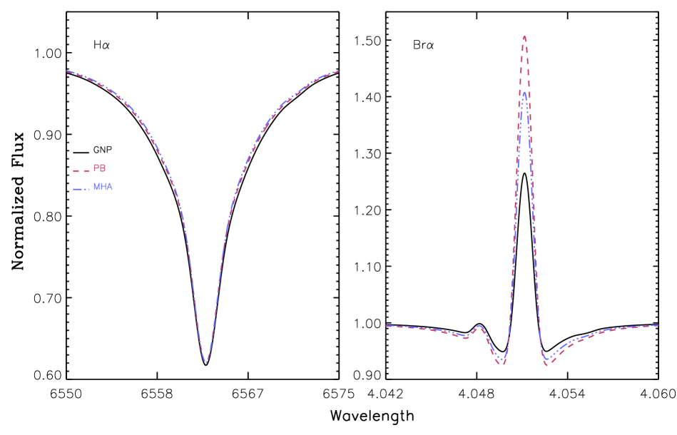
Figure 15: Influence of different collision strengths on the population of $n=4/5$ (left) and the corresponding Br_α profile (right). For comparison, we also display the changes in H_α. See text.

In summary, even in the outermost photosphere the actual value of $b_{5}/b_{4}$ is controlled by (almost) all radiative processes (with additional collisional contributions in the lower photosphere), and thus depends on a precise description of the continuum and line radiation field and to a lesser extent on the correct run of the temperature stratification (entering the recombination coefficients). Interestingly, however, we have also seen that in almost all of our simulations level 4 is more underpopulated than level 5, independent of the various processes considered. In Appendix B we will show that at least this principal behavior can be regarded as the consequence of a typical nebula-like situation, namely as due to the competition between recombination and downwards transitions.

In the wind, on the other hand, a Case B like nebula approximation is able to explain the run of all hydrogen occupation numbers alone. As it will be shown in the appendix, the actual conditions in the outer wind depend strongly on whether line-blocking/-blanketing is considered or not. In all cases, however, the abrupt decrease of the Br_α source function in the transition region between photosphere and wind is triggered by the onset of dilution and the Doppler-effect shifting the (resonance-)lines into the neighboring continuum, thus effectively pumping the excited levels.

5.2 Influence of various parameters

Collision strengths.

As already outlined, collisions do play a role in the formation of the emission peak of Br_α and, even more, in the line wings. In particular, these are the collisional ionization/recombination processes for $n\geq 3$ and the collisional excitation/deexcitation processes within transitions $i\leftrightarrow j,i\geq 3,j\geq i+1$, (strongest for $j=i+1$) which keep the occupation numbers for levels $\geq 3$ and higher in of close to LTE than expected from considering the radiative processes (for given radiation field) alone. From comparing the departure coefficients calculated with and without collisional rates, one might predict that a decrease of the collisional strengths in complete models will increase the strengths of the absorptions wings (since, around $\tau_{\rm Ross}=10^{-2}$, $b_{4}\approx b_{5}\approx 1$ compared to $b_{4}>b_{5}>1$ with and without collisions, respectively), whereas the influence on the emission is difficult to estimate. In Fig. 15, we display the result of three calculations using different sets of collision strengths and its impact on the H_α and Br_α profiles.

Our updated cmfgen “standard” model utilizes the hydrogen collision strengths from Mihalas et al. (1975) (MHA), which are compared to our previous data set from Giovanardi et al. (1987) (GNP) and recent collision strengths from Przybilla & Butler (2004) (PB). The difference between these data sets is significant, particularly for transitions with intermediate $i,j$ such as Br_α. Our “standard” MHA collision strengths lie in between the GNP and PB data sets, the latter being typically a factor of five smaller than the GNP implementation. However, the reaction of the departure coefficients seems to be small. The “only” difference is a weak increase of $b_{4}$ in the lower part of the line-forming region (as predicted above) and a weak decrease of $b_{4}$ in the outer one, i.e., the NLTE effects become increased everywhere. Consequently, the absorption wings of Br_α become deeper and the emission-peak higher, when using the data set with reduced collision strengths (PB) by Przybilla & Butler (2004) (Fig. 15, right panel, dotted profile), where the small differences in departure coefficients are (non-linearly) amplified according to Eq. 2. Since the changes in collision strengths affect both the peak of the line core and the absorption wings of Br_α, they cannot be mapped directly onto ${\dot{M}}$ variations, as the latter only modifies the line core in the thin wind case. Such changes may rather be accomplished by slightly modifying the gravity of the star.

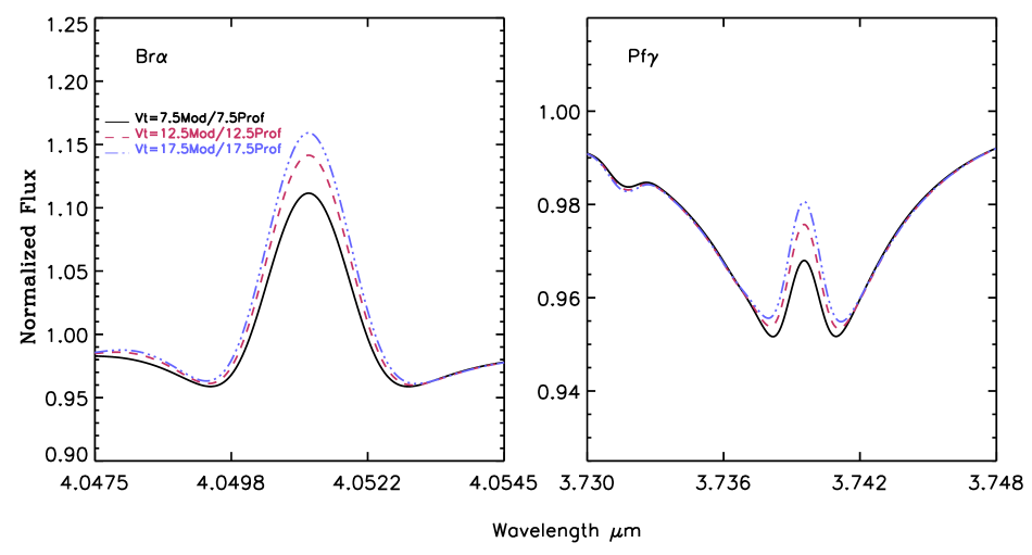
Figure 16: Influence of different microturbulent velocities on Br_α (left) and Pf_γ (right). See text.

Microturbulence.

One of the basic “unknowns” in the calculation of synthetic profiles based on model atmospheres is the microturbulent velocity, $v_{\rm{turb}}$ (e.g., Smith & Howarth 1998, Villamariz & Herrero 2000, Repolust et al. 2004, Hunter et al. 2007). Though it is possible to obtain a “compromise” estimate for this quantity from a simultaneous fit to a multitude of different lines, it is well known that different lines indicate different values, pointing to a dependence on atmospheric height. As a rule of thumb, in the parameter range considered here a value of $v_{\rm{turb}}$ on the order of 10 km s^-1 seems to be consistent with a variety of investigations. Fig. 16 compares the influence of this quantity on the synthetic Br_α profile, again by means of our model of HD 37468, and a typical mass-loss rate. Though a small impact is visible in the blue wing (due to the reaction of the Hei component), the major effect concerns the height of the emission peak, which increases for increasing $v_{\rm{turb}}$ (varied between 7.5 and 17.5 km s^-1). By comparing with Fig. 12, we see that for (very) thin winds (with the line wings well in absorption), an uncertainty in $v_{\rm{turb}}$ of $\pm$5 km s^-1 (which is a typical value) can easily induce uncertainties of a factor of two in the deduced ${\dot{M}}$. We note, however, that unlike ${\dot{M}}$ which changes “only” the height of the emission peak (see Fig. 12), microturbulence modifies both its height and width (see Fig. 16-left). A similar effect as for Br_α but with lower amplitude is found for Pf_γ (see Fig. 16-right). Therefore, provided the spectral resolution is high enough, in principle one could separate the effects of ${\dot{M}}$ and microturbulence and reduce the uncertainty in the final ${\dot{M}}$ estimate.

Most importantly, micro-turbulence affects level n= 4 (similar to the influence of the collisional strengths): The higher the turbulence, the sooner and the more effective this level becomes depopulated, increasing the line source-function. Thus, it is important to adapt $v_{\rm{turb}}$ already in the atmospheric model ($\rightarrow$ changes in the occupation numbers), and not only in the formal integral, as it is often done with respect to metallic lines and Hei.

$\beta$-law.

Here we concentrate on the effects of the steepness of the wind velocity law (expressed in terms of $\beta$) on the line profiles from thin wind objects. At first, for very thin (= weak) winds such as the one from HD 37468, there is almost no reaction at all, since the profile, particularly the line core, is not formed in the wind. For winds with a somewhat higher density (as HD 76341) where the line core of H_α already reacts, the situation is somewhat different. Figure 17 shows corresponding $L$-Band hydrogen lines together with H_α, where both $\beta$ and ${\dot{M}}$ have been modified in opposite directions to keep the H_α core at the same depth. (For this model, such a combination preserves the Br_γ core as well). Interestingly, however, the cores of Br_α and Pf_γ still react strongly, showing that these lines, together with H_α and/or Br_γ, can be confidently used to constrain both $\beta$ and ${\dot{M}}$ in objects with (not too) thin winds and to break the classical ${\dot{M}}$-$\beta$ degeneracy.

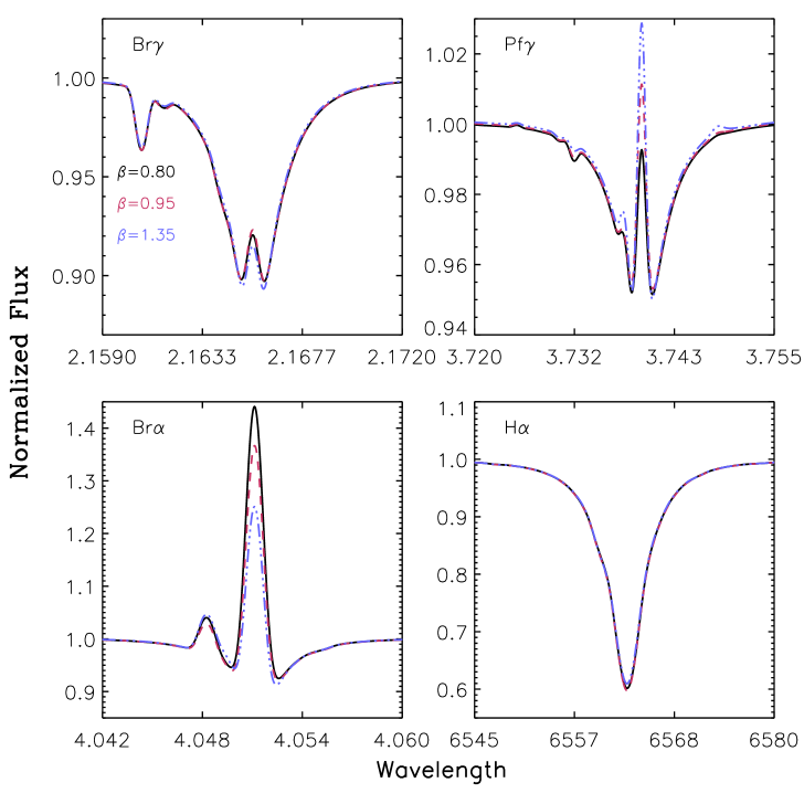
Figure 17: Influence of $\beta$ in thin wind objects (here: our model of HD 76341). Three combinations of $\beta$ and ${\dot{M}}$ which keep the H_α core at the same depth. The different sensitivity of the cores of Br_α and Pf_γ to $\beta$ breaks the well-known ${\dot{M}}$-$\beta$ degeneracy. See text.

Transition Velocity.

A variation of the transition velocity (which defines the transition from photosphere to wind) in the thin/weak wind case shows only minor effects (not displayed here) in the emission core of Br_α, provided such transition takes places at reasonable velocities (roughly between 0.05 … 0.5 V_sound). For the rest of the diagnostic lines considered here, we find no effect at all. If the transition is moved deeper into the photosphere, i.e., below 0.05 V_sound, the Br_α core starts to display a moderate sensitivity.

Finally, we investigated how Br_α and Pf_γ respond to clumping in the thin wind regime. Similarly to the dependence on the transition velocity, we found no effects, unless severe clumping is already present at the base of the photosphere, in which case minor effects start to appear in the core of Br_α.

6 Discussion

6.1 On the reliability of the derived mass-loss rates.

Since the number of ${\dot{M}}$ determinations for OB-stars has significantly increased during the last decade, and largely differing values even for the same objects can be found in the literature, it might be necessary to comment on the reliability of the data provided here. Actually, the major origin of differences in the mass-loss rates bases on different assumptions regarding the clumping properties of the wind. These range from unclumped media over microclumping (constant or stratified, with different prescriptions on the clumping-law) to the inclusion of the effects from macroclumping and vorosity.

From the comparison provided in Appendix A, it becomes obvious that in most cases the basic quantity which can be deduced from the observations, namely the optical depth invariant $Q$, is rather consistent within a variety of studies, at least when concentrating on $\rho^{2}$-dependent diagnostics. Diagnostics relying mostly on UV resonance lines are more strongly affected, as can be seen, e.g., from the differences in the corresponding $Q_{\rm res}$ value derived here and by Fullerton et al. (2006), who studied the Pv resonance line alone. Reasons for such discrepancy are (i) the influence of X-ray/EUV emission on the ionization equilibrium, particularly in the mid and outer wind (see below), and (ii) the strong impact of macroclumping/vorosity on the formation of resonance lines (Sundqvist et al. 2010, 2011, and references therein).

In this work, we have derived the stellar and wind parameters from a consistent, multi-wavelength analysis, allowing for a rather general clumping law. Since we obtained almost perfect simulations of the observed energy distributions, from the UV to the IR (and sometimes even the radio regime), we are quite confident on the quality of the provided values. Corresponding error estimates have been quoted in Sect. 3. Even admitting that the neglect of macroclumping/vorosity might influence the UV resonance lines (particularly those of intermediate strength) to a certain degree, and that our treatment of the X-ray emission is only a first approximation, the ubiquity of excellent fits to features from a variety of elements forming in different layers cannot be considered as pure coincidence. We are optimistic that problems within individual features (which can be disastrous in analyses concentrating on such features alone) have, if at all, only a mild impact in a multi-wavelength study as performed here.

One specific problem within our analysis which cannot be neglected is the problem with the cores of the optical hydrogen and HeI lines, encountered for Cyg OB2 #7 and #8A as well as for $\alpha$ Cam (but see our corresponding comment in Sect. 4). Briefly repeated, the problem reflects the fact that within our analysis we were not able to obtain a simultaneous fit for both the cores of these photospheric features and the IR-lines formed in the lower/mid wind. For a perfect fit of the IR features, a low ${\dot{M}}$ in parallel with a quite large clumping factor (CL₁ $\approx$ 0.01) is needed, whereas a fit of the photospheric line cores requires a larger ${\dot{M}}$ accompanied with moderate clumping (CL₁ $\approx$ 0.1). Further tests are certainly necessary to clarify this problem (i.e., the shape of the assumed clumping law might still not be optimum). In the meanwhile we suggest that the mass-loss rates of the problematic objects should be considered as a lower limit, and might need to be increased in future work.

Thin and weak winds.

As has been outlined in Sect. 1, the vast majority of mass-loss determinations for weak winds and weak-wind candidates has been performed by analyzing UV resonance lines, since H_α is no longer usable at low ${\dot{M}}$, and the IR has not been invoked until now.

A crucial point regarding the reliability of UV ${\dot{M}}$-determinations for weak-winded stars has been already provided by Puls et al. (2008, see their Fig. 20). They calculated the diagnostic UV and H_α profiles for a set of thin and weak wind models where the mass-loss rate was varied by almost two orders of magnitude whilst the X-ray luminosity was increased in parallel to keep the ionization structure and thus the UV lines at the observed level. The changes imposed on the wind did not reach the photospheric levels, and thus the UV iron forest did not change. Most alarming, however, is their finding that essentially all profiles could be equally well reproduced with any ${\dot{M}}$ combined with an appropriate X-ray luminosity, $L_{x}$. Thus, no independent UV mass-loss determination is feasible unless the X-ray properties of the star are accurately known.

This problem, of course, is also present in our analysis. But here, we have utilized the Br_α line as the primary ${\dot{M}}$ indicator, due to its high sensitivity on ${\dot{M}}$, being formed in the upper photosphere for weak winded stars. A similar investigation of the same ${\dot{M}}$-$L_{x}$ combinations as for the UV, but using Br_α, lead to very promising result (see Puls et al. 2008, their Fig. 22): In the case of very low ${\dot{M}}$, i.e., a deep-seated line formation region, Br_α turned out to be basically unaffected by X-rays. Even with increasing mass-loss rate, the hydrogen core of Br_α remains unaffected, at least for canonical X-ray luminosities ($L_{\rm x}/L_{\rm bol}<10^{-4})$. Changes, however, arise for the Heii emission component of Br_α, caused by the large sensitivity of the Heii/Heiii ionization equilibrium to X-rays. This problem needs to be kept in mind for future analyses.

Finally, to assess the precision of the derived mass-loss rate for our weak-wind object HD 37468, we have to consider the major sources of error, as discussed in Sect. 5.2, particularly the impact of the hydrogen bound-bound collision strengths. Here we estimate a total error of plus/minus 0.5 dex, which is irrelevant at such low mass-loss rates.

6.2 Stratification of clumping factors

Since our analysis comprises both $\rho$ and $\rho^{2}$ diagnostics (with all the caveats regarding the potential impact of macroclumping/vorosity), we are able to provide absolute values for $f_{\rm cl}(r)$ as well as for ${\dot{M}}$. This is quite different from (and superior to) the investigation by PUL06, who could derive “only” relative values (normalized to an outer wind assumed to be unclumped), because of relying on $\rho^{2}$ diagnostics alone.

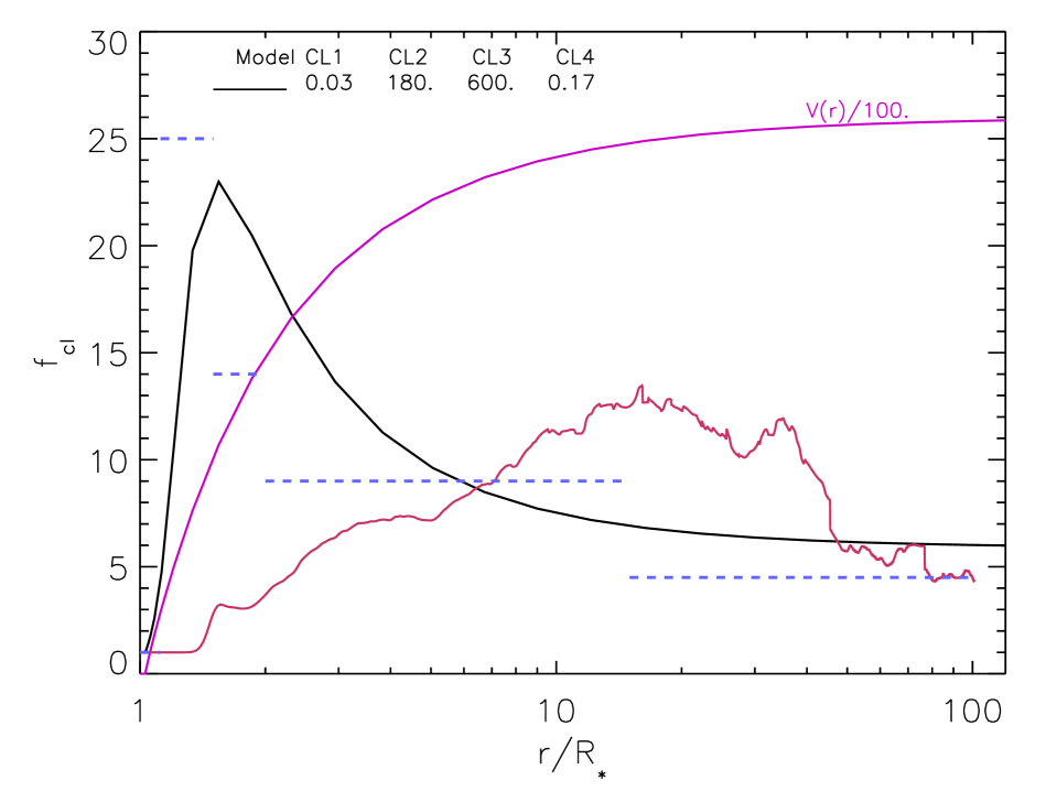
Figure 18: Radial stratification of the clumping factor, $f_{cl}$, for $\zeta$ Pup. Black solid: clumping law derived from our model fits. Red solid: Theoretical predictions by Runacres & Owocki (2002) from hydrodynamical models, with self-excited line driven instability. Dashed: Average clumping factors derived by Puls et al. (2006) assuming an outer wind matching the theoretical predictions. Magenta solid: run of the velocity field in units of 100 km s^-1. See also Sect. 4.

Dense winds.

For most of our dense wind objects, we found rather strong clumping close to the wind-base (which has a substantial impact on the actual mass-loss rate, see next subsection), whereafter the clumping factor decreases towards the mid/outer wind. This finding is similar to the results from PUL06, at least qualitatively. An even quantitative comparison is possible for the case of $\zeta$ Pup, the only star among our sample for which we could determine the run of the clumping factor throughout the entire wind (Fig. 18). When normalizing the results by PUL06 to a similar value in the outer wind ($f_{\rm cl}\approx 5$), the agreement with our results is excellent and re-assuring, since both investigations are completely independent from each other and rely on considerably different methods. Likewise re-assuring is the fact that the derived stratification of $f_{\rm cl}(r)$ is very similar to recent results by Sundqvist et al. (2011), who performed a consistent analysis of Pv and hydrogen/helium recombination lines in the O6I(n)f supergiant $\lambda$ Cep (a cooler counterpart of $\zeta$ Pup), including the consideration of macroclumping and vorosity effects. Also for this object, it turned out that clumping peaks close to the wind base, with a maximum value of $f_{\rm cl}\approx 28$, which is rather close to the value derived here for $\zeta$ Pup (see Fig 18).

Accounting as well for the previous work by Crowther et al. (2002), Hillier et al. (2003) and Bouret et al. (2003, 2005) (see Sect. 1), there is now overwhelming evidence for the presence of highly clumped material close to the wind base. These findings are in stark contrast to theoretical expectations resulting from radiation hydrodynamic simulations (Sect. 1), which predict a rather shallow increase of the clumping factor, due to the strong damping of the line instability in the lower wind caused by the so-called line-drag effect (Lucy 1984, Owocki & Rybicki 1985). In Fig 18 we compare our present results and those from PUL06 with prototypical predictions from radiation hydrodynamic simulations, here from the work by Runacres & Owocki (2002). Though there is a fair agreement for the intermediate and outer wind, the disagreement in the lower wind is striking. A similar conclusion has been reached by Sundqvist et al. (2011), and further progress on the hydrodynamic modeling seems to be necessary to understand this problem.

Thin winds.

Except for HD 217086, all our sample stars with thin winds (i.e., H_α in absorption) require no clumping to yield excellent fits, and for the former object the derived clumping is less ($f_{\rm v}=0.1$) than for the typical dense wind case. Again, this finding is in agreement with the results from PUL06, who constrained the clumping factors for thin winded objects to be similar in the inner and outer wind. Thus and in connection with our present results, one might tentatively conclude that most thin winds are rather unclumped, which immediately raises the question about the difference in the underlying physics. Might it be that the wind-instability is much stronger in objects with dense winds, e.g., due to (stronger) non-radial pulsations, or is there a connection with sub-surface convection, as suggested by Cantiello et al. (2009)?

6.3 Wind-momentum rates

Figure 19: Wind-momentum rates for our sample stars, as a function of $\log(L/L_{\odot})$. Asterisks correspond to supergiants, crosses to other luminosity classes. The two weak wind candidates HD 76341 and HD 37468 are denoted by large symbols. The solid line shows the theoretical predictions for the WLR by Vink et al. (2000), whilst the dashed one has been shifted to lower values by 0.55 dex (see text).

In Fig. 19, we plot the wind-momentum luminosity relation (WLR) for our sample stars, i.e., the wind-momentum rates, modified by the factor ($R_{\ast}$/$R_{\odot}$)^0.5, as a function of luminosity. The results of our analysis suggest a well defined relation, if we exclude three outliers, the binary Cyg OB2 #8A well above and HD 76341/HD 37468 well below the average relation. Of course, a much larger sample needs to be investigated before a final conclusion can be drawn.

From a linear regression to our results, we obtain an ‘observed’ relation in parallel to the theoretical predictions by Vink et al. (2000, solid), but 0.55 dex (factor of 3.5) lower. Due to its large deviation (2 dex!), HD 37468 is certainly a weak winded star, whereas HD 76341 (with a deviation of 0.9 dex) might be considered as a weak-wind candidate, interestingly a Ib supergiant..

On the assumption of an unclumped outer wind, PUL06 found a good agreement between their “observed” and the theoretical WLR. These results could be unified with ours on the hypothesis that the outer regions of most winds are actually clumped, with a typical clumping factor on the order of 10. With regard to our analysis of $\zeta$ Pup (and also the hydro simulations), this seems to be a reasonable, though somewhat too large value.

A down-scaling of theoretical wind-momenta as obtained here is also consistent with results from the analysis of $\lambda$ Cep by Sundqvist et al. (2011), who derived a mass-loss rate being a factor of two lower than predicted by Vink et al. (2000). Let us finally note that an independent “measurement” of the mass-loss rate of $\zeta$ Pup based on X-ray line emission by Cohen et al. (2010) resulted in a value of 3.5 $\cdot 10^{-6}\,{\rm M_{\odot}/yr}$, with a lower limit of 2.0 $\cdot 10^{-6}\,{\rm M_{\odot}/yr}$, if the abundance pattern would be solar (which is rather unlikely).

7 Summary, conclusions and future perspectives

In this pilot study, we have investigated the diagnostic potential of $L$-band spectroscopy to provide strong constraints on hot star winds, with particular emphasis on the determination of their clumping properties and (actual) mass-loss rates, even for objects with very thin (=weak) winds. To this end, we have secured $L^{(^{\prime})}$ band spectra (featuring Br_α, Pf_γ and Hei 3.703) for a sample of ten O-/early B-type stars, by means of ISAAC@VLT and SpeX@IRTF. The sample has been designed in such a way as to cover objects with both dense and thin winds, with the additional requirement that spectroscopic data in the UV, optical and $H/K$ band as well as radio observations are present and that most of the objects have been previously analyzed by means of quantitative spectroscopy.

For all stars, we performed a consistent multi-wavelength NLTE analysis by means of cmfgen, using the complete spectral information including our new $L$-band data. We assumed a microclumped wind, with a rather universal clumping law based on four parameters to be fitted simultaneously with the other stellar and wind parameters. Moreover, we accounted for rotational and macroturbulent broadening in parallel.

For the objects with dense winds, we were able to derive absolute values for mass-loss rates and clumping factors (and not only relative ones as in PUL06), where Pf_γ and Br_α proved to be invaluable tools to derive the clumping properties in the inner and mid wind, respectively.

For our objects with thin winds, on the other hand, the narrow emission core of Br_α(in combination with its line wings) proved as a powerful mass-loss indicator, due to its strong reaction even at lowest ${\dot{M}}$, its independence of X-ray emission, and its only moderate contamination by additional effects such as atomic data, microturbulence and velocity law.

Contrasted to what might be expected, the height of the Br_α line core increases with decreasing mass-loss. This is a consequence of the transition region between photosphere and wind “moving” towards lower $\tau_{\rm Ross}$ for decreasing ${\dot{M}}$, so that more and more of the strong line source function becomes “visible” when the wind becomes thinner. The origin of such a strong source function is a combination of various effects in the upper photosphere and the transonic region that depopulates the lower level of Br_α, $n=4$, stronger than the upper one, $n=5$. By detailed simulations, we explained this in terms of a nebula-like situation, due to the competition between recombinations and downwards transitions, where the stronger decay from $n=4$ (compared to the decay from $n=5$) is decisive.

As an interesting by-product, the specific sensitivity of Br_α and Pf_γ on the velocity field exponent $\beta$ in (not too) thin winds allows a break in the well-known ${\dot{M}}$-$\beta$ degeneracy when using H_α alone. On the other hand, the dependence of Br_α on $\beta$ for weak winds is negligible, which decreases the error bars of the derived ${\dot{M}}$. A major point controlling the depopulation of the lower level of Br_α and thus the height of the emission peak are the hydrogen bound-bound collisional data which are used. Our models utilize data by Mihalas et al. (1975), which provide something of a compromise regarding collisional strengths when comparing with other data sets. Overall, we estimate the error in our Br_α-${\dot{M}}$ determination of weak-winded stars by $\pm$ 0.5 dex. This is certainly better than UV diagnostics that strongly depend on the assumed description of X-ray properties and are further hampered by the impact of macroclumping and vorosity.

We compared the results of our analysis with those from previous work, in particular the derived $T_{\rm eff}$, $\log g$ and $Q$-values (the optical depth invariant(s)). With respect to $T_{\rm eff}$, the (average) agreement is significantly hampered due to sizable differences for Cyg OB2 #8C ($\Delta T_{\rm eff}\approx$ 4000 K), whereas the rest agrees within the conventional errors of $\pm$ 1000 K. The large disagreement for the former object has been attributed to differences in the derived rotational/macroturbulent velocities. On the other hand, the agreement with respect to $Q$ is satisfactory.

Almost all of our dense wind objects require large clumping close to the wind base, whereas for the thin winded stars we did not need to invoke clumping at all. Our clumping factors for the best studied object, $\zeta$ Pup, agree very well with the work by PUL06, if the clumping in the outer wind (which could not derived by the latter authors) is scaled to similar values. Moreover, our results on strong clumping in the lower wind are also consistent with other findings, particularly those by Sundqvist et al. (2011), and challenge present radiation hydrodynamic simulations which predict a much shallower increase of the clumping factors.

Because of using Br_α as a mass-loss indicator, we were able to fully characterize one weak-winded star, the O9.5 dwarf HD 37468, and one weak wind candidate, the O9Ib supergiant(!) HD 76341.

Finally, our results suggest a well defined WLR (discarding the two weak-winded objects and the binary Cyg OB2 #8A) that is located 0.55 dex below the predictions by Vink et al. (2000). From a comparison with PUL06, it seems likely that at least dense winds are considerably clumped in their outer regions. We suggest that the mass-loss rates from PUL06 are upper limits indeed, and that a downscaling of their values by factors on the order of 2 to 3 seems likely.

From all these results, we conclude that the diagnostic potential of IR $L$-band spectroscopy for deriving clumping properties and mass-loss rates of hot star winds is really promising. We suggest to extend this rather small sample with further $L$-band observations for a carefully selected sample of OB stars (with large and low ${\dot{M}}$) in order to derive statistically conclusive results on the “true” mass-loss rates from these stars. Any result drawn from only a few objects suffers from a variety of problems (e.g., the objects might be peculiar, or problems related to the diagnostic tools might remain hidden), and only a careful analysis of a large number of objects (performed with the same diagnostic tool) allows the identification of trends and outliers.

Moreover, there is the additional problem of variability. Due to its higher sensitivity to mass-loss, it might be expected that Br_α is an even better candidate than H_α (e.g., Markova et al. 2005 and references therein) to study and to analyze wind variability in dense winds. The impact of Br_α line profile variability on mass-loss/clumping diagnostics needs to be investigated as well. To our knowledge, corresponding observations have not been carried out so far, and deserve future interest. In thin winds, on the other hand, a strong variability is not to be expected, because of the near-photospheric origin of Br_α and assuming a stationary photosphere. This expectation needs to be confirmed as well, and a contradicting outcome might point to variability in the location of and the conditions in the transition zone, e.g., related to pulsations.

Finally, and from our experience accumulated so far, we are confident that Br_αwill become the primary diagnostic tool to measure very low mass-loss rates at unprecedented accuracy, thus clearly identifying weak-winded stars and quantifying the degree with which they lie below theoretical predictions.

Appendix A Detailed comparison of present results with other investigations

The present work comprises a detailed analysis of a small sample of hot stars, based on the combination of optical, NIR and UV spectra with one of the most sophisticated NLTE atmosphere codes presently available, cmfgen. Thus, a comparison of the derived results with those from more restricted investigations (with respect to wavelength range) based on alternative atmosphere codes provides an opportunity to address typical uncertainties inherent to the spectroscopic analysis of such objects, caused by different data-sets and tools. As outlined in Sect. 2 (cf. Table 1), most previous investigations of our targets have been analyzed by means of fastwind , or by (quasi-) analytic methods designed for specific diagnostics such as H_α or the IR-/mm-/radio continuum (for an overview of these methods, see Kudritzki & Puls 2000, Puls et al. 2008 and references therein).

Brief comments on important differences between our and those results have been already given in Sects. 4 and 5, and the complete set of the various stellar and wind-parameters is presented in Table 4. In the following, the various investigations are referred to following the enumeration provided at the end of this table (ref#). Note that a direct comparison of mass-loss rates is still not possible, due to the uncertainties in distances (and thus radii) for Galactic objects. Moreover, previous analyses were based on either unclumped models (ref# 2-7) or that the derived clumping factors had to be normalized to the clumping conditions in the outermost wind, which are still unclear (ref# 8). Thus, a meaningful comparison is possible only for the optical depth invariants ,

$$Q=\frac{\dot{M}}{(R_{\star}v_{\infty})^{1.5}\sqrt{f_{\rm v}}}\qquad\mbox{and}\qquad Q_{\rm res}=\frac{\dot{M}}{R_{\star}v_{\infty}^{2}},$$ (3)

which describe the actual measurement quantities related to (i) $\rho^{2}$-dependent processes ($Q$), if $f_{\rm v}$ is the average clumping factor in the corresponding formation region and the clumps are optically thin, and (ii) $\rho$-dependent processes ($Q_{\rm res}$), under the assumption that clumping plays only a minor role (but see Sect. 1).

Fig. 20 provides an impression of the differences in the most important parameters for the individual stars, by comparing the effective temperatures and gravities (upper 3$\times$3 panels), and the optical depth invariants and luminosities (lower 3$\times$3 panels). Note that all panels provide identical scales, to enable an easy visualization. From the figure, it is quite clear that typical differences in $T_{\rm eff}$ are of the order of 1,000 to 2,000 K, with corresponding differences of 0.1 to 0.2 dex in $\log g$. The largest differences are found for the effective temperature of Cyg OB2 #8C (roughly 4,000 K when comparing with ref# 3 and 6/8), which has been already discussed in Sect. 4, and most probably relates to an underestimation of $v\sin i$ in these investigations. It is reassuring that in most cases the connecting lines between our (crosses) and the other results in the $T_{\rm eff}$-$\log g$ plane have a positive slope, indicating that higher temperatures go in line with higher gravities and vice versa, which is consistent with the behavior of the gravity indicators (usually, the wings of the Balmer lines).

Table 3: Mean difference of derived effective temperature, $\Delta T_{\rm eff}=T_{\rm eff}({\rm ref\,\,i})-T_{\rm eff}({\rm this\,\,work})$ and derived optical depth invariant, $\Delta\log Q$, for $N$ objects from reference $i,i=1,8$ in common with our sample (cf. Table 4). $\Delta T_{\rm eff}$ in kK, $\Delta\log Q$ in dex. For ref# 1, we compare the $Q_{\rm res}$-values, whereas for the rest we compare the $Q$-values normalized by $f_{\rm v}$ (see Eq. 3.) Positive values indicate that the results from the specific work are on average larger than the results derived here. $\sigma$ is the dispersion of these differences. No values are given for ref# 2 (Kudritzki et al. 1999), since there is only one object in common.

ref#	$N$	$\langle\Delta T_{\rm eff}\rangle$	$\sigma(\Delta T_{\rm eff})$	$\langle\Delta\log Q\rangle$	$\sigma(\Delta\log Q)$
1	4			-1.38	0.76
3	3	1.63	1.72	-0.21	0.31
4	3	0.13	1.70	0.05	0.28
5	3	-0.57	0.59	0.11	0.28
6	4	1.75	1.79	-0.02	0.38
7	8	-0.21	1.67	-0.06∗	0.31∗
8	6			-0.08	0.23

^∗ mean difference and dispersion only for 7 objects, excluding the weak-winded object HD 37468.

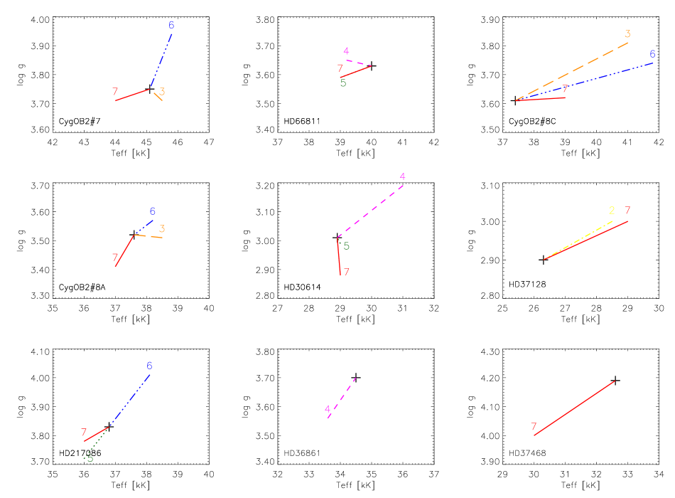
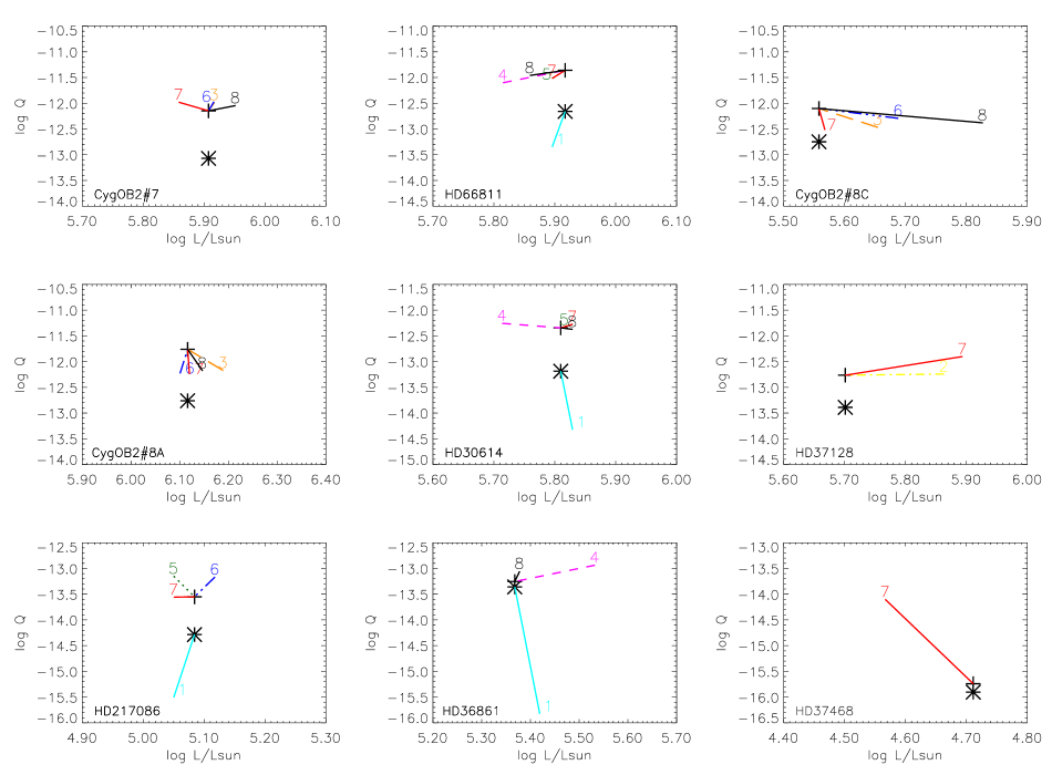
Figure 20: Comparison of the results obtained in this work (crosses) with results from other investigations (for data and reference identifiers, see Table 4). Upper 3$\times$3 panels: $\log g$ vs. $T_{\rm eff}$; all panels have the same scale, corresponding to an extent of 5000 K in $T_{\rm eff}$ and 0.4 dex in $\log g$. Lower 3$\times$3 panels: $\log Q$ vs. $\log(L/L_{\odot})$, with axes extending over 0.4 dex in $\log(L/L_{\odot})$ and 3.5 dex in $\log Q$. In order to facilitate the comparison with $\rho^{2}$-diagnostics, all $Q$ values have been normalized to $f_{\rm v}=1$ (see Eq. 3). The asterisks provide the $Q_{\rm res}$-values which have to be compared with the corresponding values from ref# 1 (Fullerton et al. 2006, $\rho$-diagnostics, but including the product with the ionization fraction of Pv). Note that all $Q_{\rm res}$ values have been scaled by a factor of 10 to fit into the individual figures.

Table 4: Comparison of stellar and wind parameters as derived in the present analysis with results from previous investigations. Units as in Table 2; optical depth invariants, $Q$ and $Q_{\rm res}$ (see Eq. 3), calculated with ${\dot{M}}$ in M${}_{\odot}\,$yr^-1, $R_{\ast}$ in $R_{\odot}$ and $v_{\rm\infty}$ in km s^-1. $f_{\rm v}$ values from this work as in Table 2, i.e., equal to CL1 (Eq. 1). $f_{\rm v}$ values from reference (8) (Puls et al. 2006)) corresponding to the clumping factors within the innermost clumped region (“region 2”) extending between $1.1\leq r/R_{\star}\leq 2$ and assuming an unclumped outer wind. For reference (1) (Fullerton et al. 2006)), the quoted results for ${\dot{M}}$ and $\log Q_{\rm res}$ include the product with the ionization fraction of Pv.

star	ref.	$T_{\rm eff}$	$\log g$	$R_{\ast}$	$Y_{\rm He}$	$v\sin i$	$v_{\rm macro}$	$v_{\rm\infty}$	${\dot{M}}$	$\beta$	$f_{\rm v}$	$\log(L/L_{\odot})$	$\log Q_{\rm res}$	$\log Q$
Cyg OB2 $\#$7	t.w.	45.1	3.75	14.7	0.13	95	65	3100	1.2	1.05	0.03	5.91	-14.07	-12.15
	3	45.5	3.71	14.6	0.30	105		3080	9.86	0.9		5.92		-11.99
	6	45.8	3.94	14.4	0.21	105		3080	9.98	0.77		5.92		-11.97
	7	44.0	3.71	14.6	0.10	145		3080	10.0			5.86		-11.98
	8	45.8	3.94	15.0	0.21	105		3080	$\leq$4.0	0.9	0.2	5.95		-12.05
HD 66811	t.w.	40.0	3.63	18.9	0.14	215	95	2250.	2.1	0.90	0.03	5.92	-13.66	-11.86
	1	39.0		19.4		219		2250	0.44	0.5		5.90	-14.35
	4	39.2	3.65	17.5	0.20	203		2300	6.4	0.92		5.82		-12.10
	5	39.0	3.59	19.4	0.20	220		2250	8.8	0.9		5.90		-12.02
	7	39.0	3.59	19.4	0.17	220		2250	8.77			5.90		-12.02
	8	39.0	3.6	18.6	0.20	220		2250	4.2	0.70	0.2	5.86		-11.96
Cyg OB2 $\#$8C	t.w.	37.4	3.61	14.3	0.10	175	90	2800	2.0	1.30	0.10	5.56	-13.75	-12.10
	3	41.0	3.81	13.3	0.09	145		2650	2.25	0.9		5.65		-12.47
	6	41.8	3.74	13.3	0.13	145		2650	3.37	0.85		5.69		-12.29
	7	39.0	3.62	13.3	0.10	145		2650	2.0			5.57		-12.52
	8	41.8	3.81	15.6	0.13	145		2650	$\leq$3.5	1.0	1.0	5.83		-12.38
Cyg OB2 $\#$8A	t.w.	37.6	3.52	26.9	0.10	110	80	2700	3.4	1.10	0.01	6.12	-13.76	-11.76
	3	38.5	3.51	27.9	0.10	95		2650	13.5	0.7		6.19		-12.17
	6	38.2	3.57	25.6	0.14	130		2650	10.4	0.74		6.10		-12.23
	7	37.0	3.41	27.9	0.10	95		2650	11.5			6.12		-12.24
	8	38.2	3.57	27.0	0.14	130		2650	$\leq$8.0	0.74	0.40	6.15		-12.18
HD 30614	t.w.	28.9	3.01	32.0	0.13	100	75	1550	0.50	1.60	0.01	5.81	-14.19	-12.34
	1	29.0		32.5		129		1550	0.037	1.0		5.83	-15.32
	4a	31.0	3.19	24.9	0.10	100		1550	4.2	1.05		5.71		-12.26
	5	29.0	2.99	32.5	0.10	100		1550	6.04	1.15		5.83		-12.27
	7	29.0	2.88	32.5	0.20	100		1550	6.0			5.83		-12.28
	8b	29.0	3.0	32.5	0.10	100		1550	2.95	1.15	0.38	5.83		-12.37
HD 37128	t.w.	26.3	2.90	34.1	0.13	55	60	1820	0.46	1.60	0.03	5.70	-14.39	-12.77
	2	28.5	3.00	35.0	0.1	80		1600	2.40	1.25		5.86		-12.74
	7	$\leq$29.0	3.0	35.0	0.1	80		1600	5.25			5.89		-12.40
HD 217086	t.w.	36.8	3.83	8.56	0.1	350	80	2510	0.028	1.2	0.10	5.08	-15.28	-13.55
	1	36.0		8.6		332		2550	$\leq$0.00174	1.0		5.05	-16.51
	5	36.0	3.72	8.6	0.15	350		2550	$\leq$0.23	0.8		5.05		-13.15
	6	38.1	4.01	8.3	0.09	350		2550	0.21	1.27		5.12		-13.17
	7	36.0	3.78	8.6	0.15	350		2550	$\leq$0.09			5.05		-13.56
HD 36861	t.w.	34.5	3.70	13.5	0.11	45	80	2175	0.28	1.3	1.0	5.37	-14.36	-13.25
	1	33.6		15.1		74		2400	0.0013	0.7		5.42	-16.83
	4	33.6	3.56	17.2	0.1	66		2400	0.97	0.8		5.53		-12.94
	8	33.6	3.56	14.4	0.10	66		2400	$\leq$0.4	0.9	0.5	5.38		-13.06
HD 76341	t.w.	32.2	3.66	21.2	0.1	63	80	1520	0.065	1.2	1.0	5.64	-14.88	-13.95
HD 37468	t.w.	32.6	4.19	7.1	0.1	35	100	1500	0.0002	0.8	1.0	4.71	-16.90	-15.74
	7c	30.0	4.0	7.1	0.1	80		2300	0.0165	1.0		4.57		-14.10

References: (1) Fullerton et al. (2006); (2) Kudritzki et al. (1999, unblanketed analysis); (3) Herrero et al. (2002); (4) Markova et al. (2004, based on stellar parameters calibrated to the results from optical NLTE analyses by ) (5) Repolust et al. (2004); (6) Mokiem et al. (2005); (7) Repolust et al. (2005); (8) Puls et al. (2006).
^a) using the high luminosity solution; ^b) stellar radius and corresponding quantities scaled to the solution by (5,7) to facilitate the comparison; ^c) stellar radius from this work.

The average differences with respect to effective temperature, $\langle\Delta T_{\rm eff}\rangle$, are presented in Table 3, discarding ref# 1 and 8 who adopted the stellar parameters, mostly from ref# 2-7. Major discrepancies seem to be present when comparing with ref# 3 and 6, who derived temperatures being on average 1,700 K higher than our results. Note, however, that a large part of this discrepancy is caused by the results obtained for Cyg OB2 #8C (see above). The other three investigations (ref# 4, 5 and 7) deviate, at least on average, much less from the present one, by a few hundreds of Kelvin. The dispersion of the differences, however, is very similar in all cases, about 1,700 K, except for ref# 5, with a dispersion of 600 K. Thus, overall, the dispersion of $\langle\Delta T_{\rm eff}\rangle$ is somewhat larger than to be expected from the typically quoted individual uncertainties of 1,000 K, which should give rise to a dispersion of 1,400 K.

Regarding the optical depth invariants, the situation is satisfactory. Except for ref# 3, the mean differences are at or below 0.1 dex (25%), with a dispersion of typically 0.3 dex (factor of 2), which is consistent with the typical individual errors (see Markova et al. 2004 for a detailed analysis). This result is particularly obvious from Fig. 20 (lower panels), where in most cases all investigations show rather similar $Q$ values.

Regarding the $Q_{\rm res}$ values which are relevant when comparing with ref# 1 (the Pv investigation by Fullerton et al. 2006), the discrepancy is still large, particularly when accounting for the fact that our results indicate considerable clumping, thus reducing the absolute mass-loss rate significantly with respect to previous investigations. On average, we find $\langle\Delta\log Q_{\rm res}\rangle\approx$-1.4 dex, with a dispersion of 0.8 dex, Thus, either (i) the actual mass-loss rates are even smaller than derived here, or (ii) the ionization fraction of Pv (remember that the results from Fullerton et al. include the product with this quantity) is very low, of the order of 4% (which would require extreme conditions in the wind, e.g., a very strong X-ray/EUV radiation field), or (iii) the line formation calculations of UV-resonance lines (both in the investigation by Fullerton et al. and in our analysis) require some additional considerations, such as the presence of optically thick clumps and/or the inclusion of a porosity in velocity space, see Sect. 1.

In summary, we conclude that at least the analysis of $Q$ seems to be well-constrained, and that different investigations give rather similar results. The remaining problem is the determination of actual mass-loss rates, which involves the “measurement” of (absolute) values of clumping factors. As we have shown in this investigation, $L$-band spectroscopy turns out to be a promising tool for this objective. Let us note that only a measurement of actual mass-loss rates will enable a strict comparison with theoretical predictions (as performed in Sect. 6), to identify present shortcomings and to provide “hard numbers” for evolutionary calculations.

The precision of effective temperatures, on the other hand, is less satisfactory. Irrespective of the fact that we did not find a real trend in the average differences with respect to three from five investigations, the dispersion is quite large, and individual discrepancies amount to intolerable values. Because of our detailed analysis covering a large range of wavelength domains and using a state-of-the-art model atmosphere code based on an “exact” treatment of all processes, we are quite confident that the $T_{\rm eff}$-errors in our work are of the order of 1,000 K or less, which means that the corresponding errors in the previous investigations must be of the order of 1,400 K or more. Additionally, two from five investigations gave a rather large average difference with respect to our results, which is alarming since all five investigations have been performed with the same NLTE atmosphere code. Insofar, recent attempts to provide reliable spectral-type-$T_{\rm eff}$-calibrations have to be augmented by results from large samples to decrease the individual scatter in a statistical way.

Appendix B Occupation numbers of the hydrogen $n=4$ and $n=5$ level in the outer atmospheres of late O-type stars with thin winds

Conditions in the outer photosphere.

As we have seen from Fig. 14, almost all of our simulations (and many more which have not been displayed) resulted in a stronger depopulation of level 4 compared to level 5 in the outer atmosphere, independent of the various processes considered. One might question how far this result can be explained (coincidence or not?). To obtain an impression on the relevant physics, we write the rate equations for level $i>1$ in the following, condensed form, again neglecting collisions, and assuming that ionization is only possible to the ground-state of the next higher ion (as it is the case for hydrogen):

$$n_{i}\sum_{i>j}A_{ij}Z_{ij}-\sum_{i<j}n_{j}A_{ji}Z_{ji}+n_{i}R_{ik}=n_{i}^{*}R_{ki},$$ (4)

where $A_{ij}$ are the Einstein-coefficients for spontaneous decay, $R_{ik}$ and $R_{ki}$ the rate-coefficients for ionization/recombination, and $Z_{ij}$ the net radiative brackets for the considered line transition, $Z_{ij}=(1-\frac{\bar{J}_{ij}}{S_{ij}})$ (the fraction denotes the ratio of mean line intensity and line source function). $n_{i}^{*}$ = $n_{k}n_{e}\Phi_{ik}(T_{e}$) denotes the LTE population of level $i$, accounting for the actual electron and ion density, $n_{e}$ and $n_{k}$ (for further details see, e.g., Mihalas 1978), such that the departure coefficients are given by $b_{i}=n_{i}/n_{i}^{*}$. Note that for purely spontaneous decays $Z_{ij}=1$, for lines which are in detailed balance, $Z_{ij}=0$, and for levels which are strongly pumped (e.g., by resonance lines with a significantly overpopulated lower level), $Z_{ij}<0$. Solving for the departure coefficients, Eq. 4 results in

$$b_{i}=\frac{\sum_{i<j}n_{j}/n_{i}^{*}A_{ji}Z_{ji}+R_{ki}}{\sum_{i>j}A_{ij}Z_{ij}+R_{ik}}.$$ (5)

The sum in the nominator corresponds to the net-contribution of lines from “above” (i.e., with upper levels $j>i$), normalized to the LTE population of the considered level, whereas the sum in the denominator is the net-contribution of lines to lower levels ($j<i$). The complete fraction can be interpreted as the ratio of populating and depopulating rates, which can be split into the contributions from bound-bound and bound-free processes,

$$b_{i}=\frac{\sum_{i<j}({\ldots})}{\sum_{i>j}({\ldots})+R_{ik}}\,+\,\frac{R_{ki}}{\sum_{i>j}({\ldots})+R_{ik}}.$$ (6)

For all our simulations 1-6 we have now calculated those two terms which determine $b_{4}$ and $b_{5}$. At first, let us concentrate on the outer photosphere, as on the right of Fig. 14. In almost all cases (except for simulation 5), the 2nd term dominates the departure coefficient, and, moreover, the first term (the ratio!, not the individual components) remains rather similar, of order 0.2. Consequently, the stronger depopulation of level 4 compared to level 5 is due to the fact that the quantity

$$\frac{R_{ki}}{\sum_{i>j}A_{ij}Z_{ij}+R_{ik}}$$ (7)

is usually larger for level 5 than for level 4, even though $R_{k5}<R_{k4}$: the accumulated transition probability from level 4 to lower levels ($A_{41}Z_{41}+A_{42}Z_{42}+A_{43}Z_{43}$) is much larger than the corresponding quantity from level 5 to lower levels ($A_{51}Z_{51}+A_{52}Z_{52}+{\ldots}$). This behavior, finally, can be traced down to the run of the oscillator-strengths in hydrogen: On the one side, e.g., $A_{41}$ is larger than $A_{51}$, etc., whereas, on the other, the corresponding net radiative brackets ($Z_{4j}$ vs. $Z_{5j}$ etc.) do not differ too much.

Two examples shall illustrate our findings. For the complete solution, the first term in Eq. 6 is roughly 0.22, whereas the 2nd term amounts to 0.62 for level 5 and to 0.53 for level 4. Thus, $b_{4}\approx 0.75$ and $b_{5}\approx 0.84$. For simulation 2, with $Z_{ij}=Z_{ji}=1$ and $R_{ik}=0$ for $i>1$, the first term $\approx 0.18$, and the 2nd one is 0.41 and 0.3, respectively, such that $b_{4}\approx 0.48$ and $b_{5}\approx 0.6$ (cf. Fig. 14).

In conclusion, the stronger depopulation of level 4 compared to level 5 in the outer photospheres of hot stars can indeed be regarded as the consequence of a typical nebula-like situation, namely as due to the competition between recombination and downwards transitions. Different approximations regarding the contributing lines do control the absolute size of the departures, but not the general trend.

Conditions in the wind.

Though the formation of the emission peak of Br_α for objects with thin winds is controlled by the processes in the upper part of the photosphere, it is also important to understand the conditions in the wind, since, as we have seen in Fig. 13, the onset of the wind prohibits a further growth of the corresponding source function: Immediately after the transition point between photosphere and wind, the source function drops to values corresponding to the local Planck-function (i.e., the departure coefficients of $n_{4}$ and $n_{5}$ become similar). Only in the outer wind the source function increases again (in contrast to the predictions of the pure H/He model, see below), which remains invisible in the profile, due to very low line optical depths. If this abrupt decrease would not happen, the monotonic behavior of the strength of the emission peak (Fig. 12) would no longer be warranted for mass-loss rates at the upper end of the scale considered here, and an important aspect of its diagnostic potential would be lost.

Let us first concentrate on the conditions in the outer wind, where the ground-state has a major impact. We stress again that we are dealing here with (very) weak winds, i.e., the continuum-edges are formed deep in the photosphere, whereas the wind and the transition region are already optically thin. Otherwise, we could no longer assume a “given” radiation temperature in the continuum, but would have to account for a simultaneous solution of radiation field and occupation numbers, as it was done, e.g., to explain the ground-state depopulation of Heii in dense hot star winds by Gabler et al. (1989).

Within our assumptions of ionizations to the ground-state of the next higher ion only and neglecting collisional processes, we obtain an alternative formulation of the rate equation for the ground-state, by summing up the rate equations for all levels $i$ (Eq. 4),

$$n_{1}R_{1k}+\sum_{i>1}n_{i}R_{ik}=n_{1}^{*}R_{k1}+\sum_{i>1}n_{i}^{*}R_{ki},$$ (8)

since the line contributions cancel out. Solving for the ground-state departure coefficient, we find

$$b_{1}=\frac{\sum_{i>1}n_{i}^{*}(R_{ki}-b_{i}R_{ik})/n_{1}^{*}\,+\,R_{k1}}{R_{1k}},$$ (9)

which can be approximated by the well known expression

$$b_{1}\approx\frac{1}{W}\frac{T_{\rm e}}{T_{\rm rad}}\exp\bigl{[}-\frac{h\nu_{0}}{k}\bigl{(}\frac{1}{T_{\rm e}}-\frac{1}{T_{\rm rad}}\bigr{)}\bigr{]}\frac{1}{\rm corr.fac.},$$ (10)

where $T_{\rm rad}$ is the radiation temperature in the ground-state (= Lyman) continuum, $\nu\geq\nu_{0}$, and $W$ the dilution factor. A correction factor of order unity accounts for the ionization/recombination from the excited levels (for details, see, e.g., Puls et al. 2005).

From here on, we have to divide between line-blocked and unblocked (e.g., pure H/He-) models, as they behave different in the wind (though similar in the outer photosphere), due to a considerably different run of electron temperature and radiation-field on both sides of the Lyman edge.

For non-blocked models (see Fig. 14), the wind-temperature is not too different from $T_{\rm rad}$, and $b_{1}$ becomes strongly overpopulated $\propto 1/W=r^{2}$. Moreover, all net radiative brackets coupled to the ground-state,

$$Z_{j1} \approx 1-W\frac{b_{1}}{b_{j}}\exp\bigl{[}\frac{h\nu_{j1}}{k}\bigl{(}\frac{1}{T_{\rm e}}-\frac{1}{T_{\rm rad,j1}}\bigr{)}\bigr{]}$$ (11)

$$\approx 1-\frac{T_{\rm e}}{T_{\rm rad}}\exp\bigl{[}\frac{h\nu_{0}}{k}\bigl{(}\frac{1}{T_{\rm rad}}-\frac{1}{T_{\rm rad,j1}}\bigr{)}\bigr{]}\frac{1}{b_{j}\,\rm{corr.fac.}}$$

become strongly negative, since (i) $b_{1}$ is severely overpopulated and (ii) the Doppler effect in the wind allows for an illumination by the continuum bluewards from the resonance-line rest-frame frequencies $\nu_{j1}$, i.e., $\bar{J}\approx WB_{\nu}(T_{\rm rad,j1})$ (optically thin (Sobolev-)approximation), with $T_{\rm rad,j1}\gg T_{\rm rad}$ due to missing line-blocking.

The consequence for the population of the excited levels (Eq. 5) is twofold. Because of the strong pumping by the resonance lines, the (normalized) population of the higher levels ($n_{j}/n_{i}^{*},j>i$) is much larger than in the photosphere, and the line term becomes larger than the recombination term. Second, the denominator decreases significantly, due to the direct effect of $Z_{j1}$ and since the the ionization rates $\propto W$ become negligible.

In total, now the first term dominates in Eq. 6, and the situation is just opposite to the conditions in the outer photosphere: The lower the considered level $i$, the larger is the nominator and the smaller the denominator, such that we obtain the sequence $b_{2}>b_{3}>b_{4}{\ldots}>1$ (cf. Fig. 14.)

For line-blocked models, on the other hand, the cooling by the enormous number of metallic lines leads to a strong decrease of the electron temperature in the outer wind, and $T_{\rm e}$ becomes much smaller than the radiation temperature in the Lyman continuum (for our late O-type model, 10,000 K vs. 25,000 K). In this case, ionization, though diluted, outweighs recombination (the exponential term in Eq. 10), and the ground-state even becomes underpopulated ($b_{1}$ $\rightarrow$0.5). Consequently, the resonance lines can no longer pump the excited levels (even more, since for blocked models the radiation temperatures close to the resonance lines, $T_{\rm rad,j1}$, are much smaller than in the unblocked case). Thus, we find a situation similar to that in the outer photosphere, namely that the 2nd term in Eq. 6 is the decisive one, and $n_{5}>n_{4}$, which is obvious also from the final increase of the line-source function for Br_α in Fig. 12 for all mass-loss rates considered.

Finally, in the region between the outer photosphere and the outer wind, the dilution of the radiation field is faster or similar to the decrease of $T_{\rm e}$, both for the blocked and the unblocked models. Thus, the departure coefficients of level 4 and 5 increase in this region (due to an overpopulated ground-state, and effective pumping due to the onset of the Doppler-shift), though at a rather similar rate, with $b_{4}\ga b_{5}$. Consequently, the source-function approaches the LTE level, which explains its abrupt decrease in the transition region.