Consistent Reconstruction of the Input
of an Oversampled Filter Bank from Noisy subbands

Abstract

This paper introduces a reconstruction approach for the input signal of an oversampled filter bank (OFB) when the sub-bands generated at its output are quantized and transmitted over a noisy channel. This approach exploits the redundancy introduced by the OFB and the fact that the quantization noise is bounded.

A maximum-likelihood estimate of the input signal is evaluated, which only considers the vectors of quantization indexes corresponding to subband signals that could have been generated by the OFB and that are compliant with the quantization errors.

When considering an OFB with an oversampling ratio of $3/2$ and a transmission of quantized subbands on an AWGN channel, compared to a classical decoder, the performance gains are up to $9$ dB in terms of SNR for the reconstructed signal, and $3$ dB in terms of channel SNR.

1 Introduction

In classical communication systems based on Shannon separation principle [1], source coding and channel coding are optimized separately. However, due to delivery delay and processing complexity constraints, source and channel coding have to be performed on short to moderate-size vectors of source samples. When the channel conditions are better than those for which the channel code has been designed, some redundancy added by the channel coder is wasted. When they are worse than expected, transmission errors may not be efficiently corrected, and will have a detrimental effect on the reconstructed bitstream, see [2].

Joint source and channel coding (JSCC) techniques have been considered to address these issues [3]. In this context, oversampled filter banks (OFB) [4, 5] are particularly interesting, since they perform a signal decomposition into subbands, leaving some controlled redundancy among subbands. When transmitted over a communication channel, subbands are usually first quantized, introducing some background quantization noise in the transmitted subbands. Quantization indexes are then packetized and transmitted over a noisy channel. In absence of residual transmission errors, the redundancy introduced by the OFB in the subband domain has been shown to be helpful to combat quantization noise [6].

When channel impairments are badly corrected by channel decoders at receiver side, corrupted packets are obtained. Classical error detection techniques, such as CRCs or checksums, check the integrity of these packets [7]. When an erroneous packet is detected, retransmission may be asked, but in delay-constrained applications, this is not always possible. The content of the packet is then lost. The robustness of OFB and more generally of frame expansions to the erasure of a whole subband has been evidenced, e.g., in [8, 9, 10]. The design freedom offered by OFB thanks to the introduced redundancy allows to construct synthesis filter banks that exploit the available samples at the receiver side to reconstruct the original signal with a minimal quadratic reconstruction error. These results have been extended in [11] to the case of several subbands randomly affected by erasures, as is the case when quantized subbands are interleaved before being packetized. A progressive missing subband estimation technique has been developed in that case.

When corrupted packets are not dropped, transmission errors result in corrupted quantization indexes, leading to subband samples corrupted by (large-variance) impulse noise. Samples not affected by transmission errors are also corrupted by (moderate-variance) quantization noise introduced at the transmitter side. A Gaussian-Bernoulli-Gaussian noise model [12] representing quite accurately the effect of quantization noise and transmission impairments has been used in [13]. Parity-check filter banks associated to the analysis OFB have been exploited to build hypotheses tests determining whether a subband is affected by a transmission impairment at some time instant. These tests rely on computing a threshold whose value depends on the ratio of the variance of the impulse noise to that of the quantization noise (Impulse over quantization noise ratio, IQNR). The samples detected as corrupted are then corrected with a Bayesian estimator. An alternative approach to detect and correct corrupted subband samples has been proposed in [14, 15] using Kalman filtering techniques. This method relies as well on a set of parameters to be chosen in advance (noise covariance matrices).

The performance of all previously mentioned techniques is strongly dependent of the characteristics of the noise model. In practice, the quantization noise is not Gaussian, but more or less uniformly distributed, and the IQNR is not that high, leading to situations where the error detection and correction is difficult.

The aim of this paper is to exploit the redundancy introduced by the OFB and to explicitly take into account the channel noise model and the bounded quantization noise. A suboptimal maximum-likelihood (ML) estimator is derived. The estimation is performed in the subspace of all consistent indexes, i.e., indexes that can result from the quantization of a subband signal belonging to the subspace of subbands that may be generated at the output of the considered OFB.

An implementation with a reasonable complexity of the proposed ML estimator is proposed. The main idea is to perform at each time instant an estimation of the vector of the most likely indexes with a sequential algorithm such as the M-algorithm [16] and then eliminate those not deemed as consistent. The consistency test is operated using interval analysis [17], but it could alternatively be done via the solution of several linear programs.

The rest of the paper is organized as follows. Section 2 describes the considered transmission scheme based on an OFB. The formulation of the optimal ML estimator of the source samples from channel outputs is given in Section 3. A suboptimal estimator is presented in Section 4 and the corresponding estimation algorithm is given in Section 5. Preliminary simulation results are shown in Section 6, before providing some conclusions.

\psfrag{b_i}[0.8]{$\mathbf{b}^{i}$}\psfrag{r_i}[0.8]{$\mathbf{r}^{i}$}\psfrag{E(z)}[1.2]{$E(z)$}\psfrag{R(z)}[1.2]{$R(z)$}\psfrag{Q}[1.2]{$Q$}\psfrag{Q^(-1)}[1.2]{$Q^{-1}$}\psfrag{z^(-1)}[0.8]{$z^{-1}$}\psfrag{x_n}[0.8]{$\mathbf{x}_{n}$}\psfrag{hx_n}[0.8]{$\widehat{\mathbf{x}}_{n}$}\psfrag{x_Ni}[0.8]{${x}_{Ni}$}\psfrag{x_Ni+1}[0.8]{${x}_{Ni+1}$}\psfrag{x_Ni+N-1}[0.8]{${x}_{Ni+N-1}$}\psfrag{x_i}[0.8]{$\mathbf{x}_{i}$}\psfrag{hx_Ni}[0.8]{$\widehat{x}_{Ni}$}\psfrag{hx_Ni+1}[0.8]{$\widehat{x}_{Ni+1}$}\psfrag{hx_Ni+N-1}[0.8]{$\widehat{x}_{Ni+N-1}$}\psfrag{y_Mi+M-1}[0.8]{${y}_{Mi+M-1}$}\psfrag{y_Mi+1}[0.8]{${y}_{Mi+1}$}\psfrag{y_Mi}[0.8]{${y}_{Mi}$}\psfrag{u_Mi+M-1}[0.8]{${u}_{Mi+M-1}$}\psfrag{u_Mi+1}[0.8]{${u}_{Mi+1}$}\psfrag{u_Mi}[0.8]{${u}_{Mi}$}\psfrag{hu_Mi+M-1}[0.8]{$\tilde{u}_{Mi+M-1}$}\psfrag{hu_Mi+1}[0.8]{$\tilde{u}_{Mi+1}$}\psfrag{hu_Mi}[0.8]{$\tilde{u}_{Mi}$}\psfrag{hy_Mi+M-1}[0.8]{$\tilde{y}_{Mi+M-1}$}\psfrag{hy_Mi+1}[0.8]{$\tilde{y}_{Mi+1}$}\psfrag{hy_Mi}[0.8]{$\tilde{y}_{Mi}$}\includegraphics[width=284.52756pt]{TransmissionScheme}

Figure 1: Transmission scheme based on an $M$-band oversampled filter bank

2 Coding and transmission scheme

Figure 1 describes a typical transmission scheme based on an $M-$band OFB with a downsampling factor of $N\leq M$, introducing a redundancy in the subbands of $M/N$. The analysis filterbank consists of $M$ FIR analysis filters $\left\{\mathbf{h}_{m}\right\}_{m=0}^{M-1}$ with maximal length $N\times(L+1)$. The corresponding polyphase representation of these filters is a $M\times N$ matrix $E(z)$. At each instant $i$, the vector $\mathbf{x}^{i}=\left(x_{Ni},\dots,x_{Ni+N-1}\right)^{T}$ is placed at the input of the OFB and the vector $\mathbf{y}^{i}=\left(y_{Mi},\dots,y_{Mi+M-1}\right)^{T}$ is obtained at its output. The relation in the temporal domain between the input and the output of the OFB is then

$$\mathbf{y}^{i}=\sum_{l=0}^{L}\mathbf{E}_{l}\mathbf{x}^{i-l}=\mathbf{E}_{L:0}\mathbf{x}^{i-L:i},$$ (1)

where $\mathbf{x}^{i-L:i}=\left(\left(\mathbf{x}^{i-L}\right)^{T},\dots,\left(\mathbf{x}^{i}\right)^{T}\right)^{T}$ contains all input samples affecting the OFB output at time $i$ and $\mathbf{E}_{L:0}=\left(\mathbf{E}_{L},\dots,\mathbf{E}_{0}\right)$ is a $M\times(L+1)N$ matrix formed by a sequence of $M\times N$ matrices $\mathbf{E}_{l},\mbox{ }l=0,\dots,L$ that can be constructed from $\left\{\mathbf{h}_{m}\right\}_{m=0}^{M-1}$ [18]. Since $E\left(z\right)$ represents a FIR filter bank, one can find a $\left(M-N\right)\times M$ polyphase matrix $P\left(z\right)$ such that $P\left(z\right)E\left(z\right)=0\>\>\>\>\forall z\in\mathbb{C}$ and that represents a FIR parity-check filter bank, see Proposition 1 in [13]. One can then write

$$P\left(z\right)=\sum_{l=0}^{L^{\prime}}\mathbf{P}_{l}z^{-l}.$$ (2)

Since $P\left(z\right)E\left(z\right)=0$, one has

$$\sum_{l=0}^{L^{\prime}}\mathbf{P}_{l}\mathbf{y}^{i-l}=\mathbf{P}_{L^{\prime}:0}\mathbf{y}^{i-L^{\prime}:i}=\mathbf{0},$$ (3)

where $\mathbf{y}^{i-L^{\prime}:i}=\left(\left(\mathbf{y}^{i-L^{\prime}}\right)^{T},\dots,\left(\mathbf{y}^{i}\right)^{T}\right)^{T}$. This property allows to determine whether a subband signal may be obtained at the output of an OFB.

For the transmission, each component $y_{Mi+m}$, $m=0,\dots,M-1$, of the vector $\mathbf{y}^{i}$ is quantized using a scalar quantizer with a step-size $\Delta_{m}$. The resulting quantization indexes $u_{Mi+m}$ are binarized to get a sequence $\mathbf{b}_{Mi+m}=\mathbf{b}(u_{Mi+m})$ of $R_{m}$ bits. The whole vector $\mathbf{u}^{i}=\left(u_{Mi},\dots,u_{Mi+M-1}\right)^{T}$ of quantized indexes is then represented by a binary sequence $\mathbf{b}^{i}=\left(\mathbf{b}^{T}_{Mi},\dots,\mathbf{b}^{T}_{Mi+M-1}\right)$ of $\sum_{m=0}^{M-1}R_{m}$ bits that are BPSK modulated and then transmitted over a memoryless channel with a transition probability $g\left(r|b\right)$. A vector $\mathbf{r}^{i}=\left(\mathbf{r}^{T}_{Mi},\dots,\mathbf{r}^{T}_{Mi+M-1}\right)^{T}$ of binary-, real- , or complex-valued samples is finally obtained at channel output.

A classical decoder would perform a hard decision on $\mathbf{r}^{i}$ to get some estimate $\widetilde{\mathbf{u}}^{i}$ of $\mathbf{u}^{i}$. After inverse quantization of $\widetilde{\mathbf{u}}^{i}$, the received subbands $\widetilde{\mathbf{y}}^{i}$ are obtained. Finally, the reconstruction is performed using the pseudo-inverse of the $E(z)$, whose polyphase representation $R(z)=(E(z)^{T}E(z))^{-1}E(z)^{T}$ is a $N\times M$ matrix such that $R(z)E(z)=I_{N\times N}$, where $I_{N\times N}$ is the $N\times N$ identity matrix. Nevertheless, this estimator may produce estimated subbands $\widetilde{\mathbf{y}}^{i}$ which may not be produced by the considered OFB. The proposed estimator addresses this issue.

3 Optimal ML estimator

At receiver side the ML estimate of the input vector at time $i$ assuming that all channel outputs have been gathered in a vector $\mathbf{r}$ is

$$\widehat{\mathbf{x}}^{i}=\arg\max_{\widetilde{\mathbf{x}}^{i}\in[\mathbf{x}]}p(\mathbf{r}|\widetilde{\mathbf{x}}^{i}),$$ (4)

where $\left[\mathbf{x}\right]$ is a vector of intervals (or box) to which all the vectors $\mathbf{x}^{i}$ are known to belong. The box $\left[\mathbf{x}\right]$ may be obtained from the dynamic of the input signal. It is aussmed to be known a priori by the receiver. Since the channel is memoryless and the maximal length of the impulse response of the analysis filters is $N\times(L+1)$ one gets

$$\widehat{\mathbf{x}}^{i}=\arg\max_{\widetilde{\mathbf{x}}^{i}\in[\mathbf{x}]}p(\mathbf{r}^{i:i+L}|\widetilde{\mathbf{x}}^{i})$$ (5)

where $\mathbf{r}^{i:i+L}=\left(\left(\mathbf{r}^{i}\right)^{T},\dots,\left(\mathbf{r}^{i+L}\right)^{T}\right)^{T}$. Let $\mathcal{U}$ be the set of all vectors $\widetilde{\mathbf{u}}^{i}$ of indexes that may be obtained at the output of the quantizers. This set, containing at most $\prod_{m=0}^{M-1}2^{R_{m}}$ elements, is independent of $i$ since the characteristics of the scalar quantizers do not depend on time. Then, the conditional probability in (5) becomes

$$\begin{split}p\left(\mathbf{r}^{i:i+L}|\widetilde{\mathbf{x}}^{i}\right)&=\sum_{\widetilde{\mathbf{u}}^{i:i+L}\in\mathcal{U}^{L+1}}p\left(\mathbf{r}^{i:i+L},\widetilde{\mathbf{u}}^{i:i+L}|\widetilde{\mathbf{x}}^{i}\right),\\ &=\sum_{\widetilde{\mathbf{u}}^{i:i+L}\in\mathcal{U}^{L+1}}p\left(\mathbf{r}^{i:i+L}|\widetilde{\mathbf{u}}^{i:i+L},\widetilde{\mathbf{x}}^{i}\right)p\left(\widetilde{\mathbf{u}}^{i:i+L}|\widetilde{\mathbf{x}}^{i}\right)\end{split}$$ (6)

The channel output $\mathbf{r}^{i:i+L}$ depends only on the channel input $\widetilde{\mathbf{u}}^{i:i+L}$. Hence, $\widetilde{\mathbf{x}}^{i}$ does not provide any additional knowledge on $\mathbf{r}^{i:i+L}$ once $\widetilde{\mathbf{u}}^{i:i+L}$ is known, $i.e.$, $\widetilde{\mathbf{x}}^{i}\longleftrightarrow\widetilde{\mathbf{u}}^{i:i+L}\longleftrightarrow\mathbf{r}^{i:i+L}$ forms a Markov chain. Then (6) becomes

$$p\left(\mathbf{r}^{i:i+L}|\widetilde{\mathbf{x}}^{i}\right)=\sum_{\widetilde{\mathbf{u}}^{i:i+L}\in\mathcal{U}^{L+1}}p\left(\mathbf{r}^{i:i+L}|\widetilde{\mathbf{u}}^{i:i+L}\right)p\left(\widetilde{\mathbf{u}}^{i:i+L}|\widetilde{\mathbf{x}}^{i}\right)$$ (7)

Using the fact that the channel is memoryless, the first term $p\left(\mathbf{r}^{i:i+L}|\widetilde{\mathbf{u}}^{i:i+L}\right)$ of (7) is easily obtained from the channel transition probability

$$\begin{split}p\left(\mathbf{r}^{i:i+L}|\widetilde{\mathbf{u}}^{i:i+L}\right)&=\prod_{\ell=0}^{L}p(\mathbf{r}^{i+\ell}|\widetilde{\mathbf{u}}^{i+\ell})\\ &=\prod_{\ell=0}^{L}\hskip 8.5359pt\prod_{m=0}^{M-1}p(\mathbf{r}_{M(i+\ell)+m}|\widetilde{u}_{M(i+\ell)+m}),\\ &=\prod_{\ell=0}^{L}\hskip 8.5359pt\prod_{m=0}^{M-1}g(\mathbf{r}_{M(i+\ell)+m}|\mathbf{b}(\widetilde{u}_{M(i+\ell)+m})).\end{split}$$ (8)

The term $g(\mathbf{r}_{M(i+\ell)+m}|\mathbf{b}(\widetilde{u}_{M(i+\ell)+m}))$ of (8) is then obtained as the product of $R_{m}$ channel transition probabilities corresponding to the $R_{m}$ bits in $\mathbf{b}(\widetilde{u}_{M(i+\ell)+m})$.

The second term $p\left(\widetilde{\mathbf{u}}^{i:i+L}|\widetilde{\mathbf{x}}^{i}\right)$ of (7) is much more complex to evaluate. Moreover, the number of terms of the sum in (7) is in general prohibitively large. A suboptimal estimator is thus introduced in the next section.

4 Suboptimal ML estimator

A suboptimal ML estimator for $\mathbf{x}^{i}$ is obtained when considering only the channel output at time $i$. Thus, one gets

$$\hat{\mathbf{x}}^{i}=\arg\max_{\widetilde{\mathbf{x}}^{i}\in[\mathbf{x}]}p(\mathbf{r}^{i}|\widetilde{\mathbf{x}}^{i})$$ (9)

and

$$\begin{split}p\left(\mathbf{r}^{i}|\widetilde{\mathbf{x}}^{i}\right)&=\sum_{\widetilde{\mathbf{u}}^{i}\in\mathcal{U}}p\left(\mathbf{r}^{i}|\widetilde{\mathbf{u}}^{i}\right)p\left(\widetilde{\mathbf{u}}^{i}|\widetilde{\mathbf{x}}^{i}\right)\end{split}$$ (10)

To evaluate $p\left(\widetilde{\mathbf{u}}^{i}|\widetilde{\mathbf{x}}^{i}\right)$, one knows that a vector of quantized indexes $\widetilde{\mathbf{u}}^{i}$ is produced when the value $\mathbf{y}^{i}$ taken by the random vector $\mathbf{Y}^{i}$ of OFB outputs belongs to some box $\left[\mathbf{y}^{i}\left(\widetilde{\mathbf{u}}^{i}\right)\right]=\left[\mathbf{y}^{i}\left(\widetilde{\mathbf{u}}^{i}\right)-\frac{\mathbf{\Delta}}{2},\mathbf{y}^{i}\left(\widetilde{\mathbf{u}}^{i}\right)+\frac{\mathbf{\Delta}}{2}\right]$, where $\mathbf{y}^{i}\left(\widetilde{\mathbf{u}}^{i}\right)$ is obtained from inverse quantization of $\widetilde{\mathbf{u}}^{i}$ and $\mathbf{\Delta}=\left(\Delta_{1},\dots,\Delta_{M}\right)^{T}$. Then

$$p\left(\mathbf{r}^{i}|\mathbf{X}^{i}=\widetilde{\mathbf{x}}^{i}\right)=\sum_{\widetilde{\mathbf{u}}^{i}\in\mathcal{U}}p\left(\mathbf{r}^{i}|\widetilde{\mathbf{u}}^{i}\right)p\left(\mathbf{Y}^{i}\in\left[\mathbf{y}^{i}\left(\widetilde{\mathbf{u}}^{i}\right)\right]|\mathbf{X}^{i}=\widetilde{\mathbf{x}}^{i}\right),$$ (11)

where $\mathbf{X}^{i}$ is the random vector at the input of the analysis OFB. One may show that the second term of (11) may be written as

$$p\left(\mathbf{Y}^{i}\in\left[\mathbf{y}^{i}\left(\widetilde{\mathbf{u}}^{i}\right)\right]|\widetilde{\mathbf{x}}^{i}\right)$$

$$= \int\limits_{\left[\mathbf{x}\right]^{L}}p\left(\mathbf{Y}^{i}\in\left[\mathbf{y}^{i}\left(\widetilde{\mathbf{u}}^{i}\right)\right],\widetilde{\mathbf{x}}^{i-L:i-1}|\widetilde{\mathbf{x}}^{i}\right)d\widetilde{\mathbf{x}}^{i-L:i-1}$$

$$= \int\limits_{\left[\mathbf{x}\right]^{L}}p\left(\mathbf{E}_{L:0}\mathbf{X}^{i-L:i}\in\left[\mathbf{y}^{i}\left(\widetilde{\mathbf{u}}^{i}\right)\right]|\widetilde{\mathbf{x}}^{i-L:i}\right)p\left(\widetilde{\mathbf{x}}^{i-L:i-1}|\widetilde{\mathbf{x}}^{i}\right)d\widetilde{\mathbf{x}}^{i-L:i-1}$$

Then, (9) becomes

$$\hat{\mathbf{x}}^{i}=\arg\max_{\widetilde{\mathbf{x}}^{i}\in[\mathbf{x}]}\sum_{\widetilde{\mathbf{u}}^{i}\in\mathcal{U}}p\left(\mathbf{r}^{i}|\widetilde{\mathbf{u}}^{i}\right)\int\limits_{\left[\mathbf{x}\right]^{L}}f\left(\widetilde{\mathbf{u}}^{i},\widetilde{\mathbf{x}}^{i-L:i}\right)p\left(\widetilde{\mathbf{x}}^{i-L:i-1}|\widetilde{\mathbf{x}}^{i}\right)d\widetilde{\mathbf{x}}^{i-L:i-1},$$

where $f\left(\widetilde{\mathbf{u}}^{i},\widetilde{\mathbf{x}}^{i-L:i}\right)=p\left(\mathbf{E}_{L:0}\mathbf{X}^{i-L:i}\in\left[\mathbf{y}^{i}\left(\widetilde{\mathbf{u}}^{i}\right)\right]|\widetilde{\mathbf{x}}^{i-L:i}\right)$. For a specific value $\widetilde{\mathbf{u}}^{i}$ one has

$$f\left(\widetilde{\mathbf{u}}^{i},\widetilde{\mathbf{x}}^{i-L:i}\right)=\begin{cases}1&\mbox{if $\mathbf{E}_{L:0}\mathbf{\widetilde{x}}^{i-L:i}\in\left[\mathbf{y}^{i}\left(\widetilde{\mathbf{u}}^{i}\right)\right]$}\\ 0&\mbox{otherwise.}\end{cases}$$

The term $f\left(\widetilde{\mathbf{u}}^{i},\widetilde{\mathbf{x}}^{i-L:i}\right)$ accounts for the fact that all values in $\mathcal{U}$ cannot be obtained at the quantized output of the OFB. One then obtains

$$\hat{\mathbf{x}}^{i}=\arg\max_{\widetilde{\mathbf{x}}^{i}\in[\mathbf{x}]}\sum_{\widetilde{\mathbf{u}}^{i}\in\mathcal{U}}p\left(\mathbf{r}^{i}|\widetilde{\mathbf{u}}^{i}\right)\int\limits_{\mathcal{S}\left(\widetilde{\mathbf{u}}^{i},\widetilde{\mathbf{x}}^{i}\right)}p\left(\widetilde{\mathbf{x}}^{i-L:i-1}|\widetilde{\mathbf{x}}^{i}\right)d\widetilde{\mathbf{x}}^{i-L:i-1},$$ (12)

where

$$\mathcal{S}\left(\widetilde{\mathbf{u}}^{i},\widetilde{\mathbf{x}}^{i}\right)=\left\{\widetilde{\mathbf{x}}^{i-L:i-1}\in\left[\mathbf{x}\right]^{L}|\mathbf{E}_{L:0}\mathbf{\widetilde{x}}^{i-L:i}\in\left[\mathbf{y}^{i}\left(\widetilde{\mathbf{u}}^{i}\right)\right]\right\}$$

Assume further that the estimation process in the previous instants $j=i-L,\dots,i-1$ has been able to provide boxes $\left[\widehat{\mathbf{x}}^{j}\right]$ such that $\mathbf{x}^{j}\in\left[\widehat{\mathbf{x}}^{j}\right]$. Then, (12) becomes

$$\begin{split}\hat{\mathbf{x}}^{i}&=\arg\max_{\widetilde{\mathbf{x}}^{i}\in[\mathbf{x}]}\sum_{\widetilde{\mathbf{u}}^{i}\in\mathcal{U}}p\left(\mathbf{r}^{i}|\widetilde{\mathbf{u}}^{i}\right)\int\limits_{\left[\widehat{\mathbf{x}}^{i-L:i-1}\right]\cap\mathcal{S}\left(\widetilde{\mathbf{u}}^{i},\widetilde{\mathbf{x}}^{i}\right)}p\left(\widetilde{\mathbf{x}}^{i-L:i-1}|\widetilde{\mathbf{x}}^{i}\right)d\widetilde{\mathbf{x}}^{i-L:i-1}\end{split}$$ (13)

Consider now for each $\widetilde{\mathbf{u}}^{i}\in\mathcal{U}$ the set

$$\mathcal{X}^{i}\left(\widetilde{\mathbf{u}}^{i}\right) = \left\{\widetilde{\mathbf{x}}^{i}\in[\mathbf{x}]|\left[\widehat{\mathbf{x}}^{i-L:i-1}\right]\cap\mathcal{S}\left(\widetilde{\mathbf{u}}^{i},\widetilde{\mathbf{x}}^{i}\right)\neq\emptyset\right\}$$

$$= \left\{\widetilde{\mathbf{x}}^{i}\in[\mathbf{x}]|\exists\widetilde{\mathbf{x}}^{i-L:i-1}\in\left[\widehat{\mathbf{x}}^{i-L:i-1}\right]\right.$$

$$\left.\mbox{ such that }E_{0}\mathbf{\widetilde{x}}^{i}\in\left[\mathbf{y}^{i}\left(\widetilde{\mathbf{u}}^{i}\right)\right]-\mathbf{E}_{L:1}\widetilde{\mathbf{x}}^{i-L:i-1}\right\}$$

This set contains all values of the input vector at time $i$ for which there exists some value of the preceding input vectors that leads to quantized OFB output indexes represented by $\widetilde{\mathbf{u}}^{i}$. $\mathcal{X}^{i}\left(\widetilde{\mathbf{u}}^{i}\right)$ is either empty or is a polytope [19]. The set $\mathcal{U}$ can be then partitioned into two subsets $\mathcal{U}_{0}=\left\{\widetilde{\mathbf{u}}^{i}\in\mathcal{U}|\mathcal{X}^{i}\left(\widetilde{\mathbf{u}}^{i}\right)=\emptyset\right\}$ and $\mathcal{U}_{1}=\left\{\widetilde{\mathbf{u}}^{i}\in\mathcal{U}|\mathcal{X}^{i}\left(\widetilde{\mathbf{u}}^{i}\right)\neq\emptyset\right\}$. Therefore (13) becomes

$$\hat{\mathbf{x}}^{i}=\arg\max_{\widetilde{\mathbf{x}}^{i}\in[\mathbf{x}]}\sum_{\widetilde{\mathbf{u}}^{i}\in\mathcal{U}_{1}}p\left(\mathbf{r}^{i}|\widetilde{\mathbf{u}}^{i}\right)\int\limits_{\left[\widehat{\mathbf{x}}^{i-L:i-1}\right]\cap\mathcal{S}\left(\widetilde{\mathbf{u}}^{i},\widetilde{\mathbf{x}}^{i}\right)}p\left(\widetilde{\mathbf{x}}^{i-L:i-1}|\widetilde{\mathbf{x}}^{i}\right)d\widetilde{\mathbf{x}}^{i-L:i-1}.$$ (14)

4.1 Other approximations

In (14), instead of considering all terms of the sum over all $\widetilde{\mathbf{u}}^{i}\in\mathcal{U}_{1}$, we only consider the term corresponding to

$$\hat{\mathbf{u}}^{i}=\arg\max_{\widetilde{\mathbf{u}}^{i}\in\mathcal{U}_{1}}p\left(\mathbf{r}^{i}|\widetilde{\mathbf{u}}^{i}\right).$$ (15)

This is the ML estimate of the quantized indexes at time $i$ accounting for the fact that $\hat{\mathbf{u}}^{i}\in\mathcal{U}_{1}$, i.e., that it can be obtained as a quantized output of the considered OFB. The classical ML estimate would consider a maximization over $\mathcal{U}$ in (15). Using (15), (14) becomes then

$$\hat{\mathbf{x}}^{i}=\arg\max_{\widetilde{\mathbf{x}}^{i}\in[\mathbf{x}]}\int\limits_{\left[\widehat{\mathbf{x}}^{i-L:i-1}\right]\cap\mathcal{S}\left(\hat{\mathbf{u}}^{i},\widetilde{\mathbf{x}}^{i}\right)}p\left(\widetilde{\mathbf{x}}^{i-L:i-1}|\widetilde{\mathbf{x}}^{i}\right)d\widetilde{\mathbf{x}}^{i-L:i-1}.$$ (16)

where the integral in (16) vanishes when $\widetilde{\mathbf{x}}^{i}\notin\mathcal{X}^{i}\left(\mathbf{\hat{u}}^{i}\right)$.

Evaluating the function to maximize in (16) is still complicated. Thus, one evaluates the set of values $\mathcal{X}^{i}\left(\mathbf{\hat{u}}^{i}\right)$ on which the interval does not vanish, or more precisely an outer-approximation of this set. Considering some $\mathbf{\widetilde{u}}^{i}\in\mathcal{U}$, an outer approximation $\left[\mathbf{x}^{i}\left(\mathbf{\widetilde{u}}^{i}\right)\right]$ of $\mathcal{X}^{i}\left(\mathbf{\widetilde{u}}^{i}\right)$ may be evaluated in several ways. One may consider solving several linear programming problems, or using tools from interval analysis [17]. If an empty outer-approximation is obtained for some $\widetilde{\mathbf{u}}^{i}$, then $\widetilde{\mathbf{u}}^{i}\notin\mathcal{U}_{1}$. This allows to construct an iterative algorithm that evaluates at each $i$ the most likely vectors of indexes and keeps only the most likely one which also belongs to $\mathcal{U}_{1}$.

4.2 Parity-check test (PCT)

To determine whether some vector of indexes belongs to $\mathcal{U}_{1},$ one may alternatively use the parity-check polyphase matrix $P\left(z\right)$. One knows that if $\mathbf{y}^{i-L^{\prime}:i}$ contains only vectors corresponding to the output of the OFB with polyphase matrix $E\left(z\right)$, then (3) is necessarily satisfied. Consider now a box $\left[\mathbf{y}^{i-L^{\prime}:i}\right]$. If $\mathbf{0}\notin\mathbf{P}_{L^{\prime}:0}\left[\mathbf{y}^{i-L^{\prime}:i}\right],$ then, there cannot be any sequence of $L^{\prime}$ vectors $\mathbf{y}^{i-L^{\prime}:i}\in\left[\mathbf{y}^{i-L^{\prime}:i}\right]$ such that $\mathbf{y}^{i-L^{\prime}:i}$ is the output of the OFB with polyphase matrix $E\left(z\right)$. This allows to build a quick test to determine whether $\left[\mathbf{y}^{i}\left(\widetilde{\mathbf{u}}^{i}\right)\right]$ may contain an OFB output at time $i$ and consequently whether $\widetilde{\mathbf{u}}^{i}$ has to be further considered. For that purpose, a box $\left[\widehat{\mathbf{y}}^{i-L^{\prime}:i-1}\right]$ containing previously verified outputs has to be available. Then, for some $\widetilde{\mathbf{u}}^{i}$, if

$$\mathbf{0}\notin\sum_{l=1}^{L^{\prime}}\mathbf{P}_{l}\left[\mathbf{\widehat{y}}^{i-l}\right]+\mathbf{P}_{0}\left[\mathbf{y}^{i}\left(\widetilde{\mathbf{u}}^{i}\right)\right]$$ (17)

then $\widetilde{\mathbf{u}}^{i}$ does not belong to $\mathcal{U}_{1}$.

The proposed algorithm is described in Section 5.

5 Estimation algorithm

This section describes the OFB input signal estimation algorithm using the signal measured at channel output.

1. Input: $\left[\mathbf{\widehat{x}}^{i-L:i-1}\right]$, $\left[\mathbf{\widehat{y}}^{i-L^{\prime}:i-1}\right]$, Output: $\left[\mathbf{\widehat{x}}^{i}\right]$, $\left[\mathbf{\widehat{y}}^{i}\right]$.

2. Initilization: $k=1$ ; $\ell=1$ ; $\mathcal{L}_{cand}^{\mathcal{U}_{1}}=\emptyset$.

3. Sort the vectors of indexes $\widetilde{\mathbf{u}}^{i}$ in the decreasing likelihood $p\left(\mathbf{r}^{i}|\widetilde{\mathbf{u}}^{i}\right)$. Keep the $N_{\max}$ most likely candidates $\mathcal{L}_{cand}=\left\{\widetilde{\mathbf{u}}^{i}\left(1\right),\dots,\widetilde{\mathbf{u}}^{i}\left(N_{\max}\right)\right\}$.

4. Do

   1. Evaluate $\left[\mathbf{x}^{i}\left(\widetilde{\mathbf{u}}^{i}\left(k\right)\right)\right]\subset[\mathbf{x}]$ satisfying $\mathbf{E}_{0}\left[\mathbf{x}^{i}\left(\widetilde{\mathbf{u}}^{i}\left(k\right)\right)\right]\subset\left[\mathbf{y}^{i}\left(\widetilde{\mathbf{u}}^{i}\left(k\right)\right)\right]-\mathbf{E}_{L:1}\left[\mathbf{\widehat{x}}^{i-L:i-1}\right]$.

   2. If $\left[\mathbf{x}^{i}\left(\widetilde{\mathbf{u}}^{i}\left(k\right)\right)\right]\neq\emptyset$ then $\mathcal{L}_{cand}^{\mathcal{U}_{1}}=\left\{\mathcal{L}_{cand}^{\mathcal{U}_{1}},\widetilde{\mathbf{u}}^{i}\left(k\right)\right\}$

   3. $k=k+1$;

5. while $k\leq N_{\max}$;

6. If $\mathcal{L}_{cand}^{\mathcal{U}_{1}}=\emptyset$ then $\left[\mathbf{\widehat{x}}^{i}\right]=\left[\mathbf{x}^{i}\left(\widetilde{\mathbf{u}}^{i}\left(1\right)\right)\right]$ ; $\widehat{\mathbf{u}}^{i}=\widetilde{\mathbf{u}}^{i}\left(1\right)$; Indicate an error. End.
   Else $N_{\max}^{\mathcal{U}_{1}}=\left|\mathcal{L}_{cand}^{\mathcal{U}_{1}}\right|$;

7. Do

8. Apply the parity-check test on $\left[\mathbf{y}^{i}\left(\mathcal{L}_{cand}^{\mathcal{U}_{1}}\left(l\right)\right)\right]$

   1. If $\mathbf{0}\in\sum_{l=1}^{L^{\prime}}\mathbf{P}_{l}\left[\mathbf{\widehat{y}}^{i-l}\right]+\mathbf{P}_{0}\left[\mathbf{y}^{i}\left(\mathcal{L}_{cand}^{\mathcal{U}_{1}}\left(l\right)\right)\right]$, then $\left[\mathbf{\widehat{x}}^{i}\right]=\left[\mathbf{x}^{i}\left(\mathcal{L}_{cand}^{\mathcal{U}_{1}}\left(l\right)\right)\right]$, $\left[\mathbf{\widehat{y}}^{i}\right]=\left[\mathbf{y}^{i}\left(\mathcal{L}_{cand}^{\mathcal{U}_{1}}\left(l\right)\right)\right],$ $\widehat{\mathbf{u}}^{i}=\mathcal{L}_{cand}^{\mathcal{U}_{1}}\left(l\right)$; End.

   2. Else $l=l+1$;

9. while $l\leq N_{\max}^{\mathcal{U}_{1}}$.

10. $\left[\mathbf{\widehat{x}}^{i}\right]=\left[\mathbf{x}^{i}\left(\mathcal{L}_{cand}^{\mathcal{U}_{1}}\left(1\right)\right)\right]$, $\left[\mathbf{\widehat{y}}^{i}\right]=\left[\mathbf{y}^{i}\left(\mathcal{L}_{cand}^{\mathcal{U}_{1}}\left(1\right)\right)\right],\widehat{\mathbf{u}}^{i}=\mathcal{L}_{cand}^{\mathcal{U}_{1}}\left(1\right)$, Indicate an error. End.

In the first call of the algorithm ($i=1$), the vectors $\left[\mathbf{\widehat{x}}^{j}\right]$$,\mbox{ $j=i-L,\dots,i-1$}$ and $\left[\mathbf{\widehat{y}}^{j}\right]$, $j=i-L^{\prime},\dots$,$i-1$ are initialized to $\left[\mathbf{0},\mathbf{0}\right]$.

Step 3. can be performed with an M-algorithm [16].

Step 4a. may be performed using linear programming or interval analysis [17]. In the latter case, the problem is to enclose the $n-$ dimensional polytope $\mathcal{X}^{i}\left(\mathbf{\widetilde{u}}^{i}\right)$ by an $n-$ dimensional box $\left[\mathbf{x}^{i}\left(\mathbf{\widetilde{u}}^{i}\right)\right]$. The box $\left[\mathbf{x}^{i}\left(\mathbf{\widetilde{u}}^{i}\right)\right]$ is an outer approximation of $\mathcal{X}^{i}\left(\mathbf{\widetilde{u}}^{i}\right)$.

At step 6., $\mathcal{L}_{cand}^{\mathcal{U}_{1}}$ contains the most likely vectors of indexes $\widetilde{\mathbf{u}}^{i}$ for which one was not able to prove that they are not in $\mathcal{U}_{1}.$ The PCT is then applied to eliminate some candidates in $\mathcal{L}_{cand}^{\mathcal{U}_{1}}$.

The most likely vector of indices $\widehat{\mathbf{u}}^{i}\in\mathcal{U}_{1}$ is then obtained in the output of the algorithm as well as $\left[\mathbf{x}^{i}\left(\mathbf{\widehat{u}}^{i}\right)\right]$ and a box $\left[\mathbf{\widehat{y}}^{i}\right]=\left[\mathbf{y}^{i}\left(\widehat{\mathbf{u}}^{i}\right)\right]$ containing the noise-free OFB output at time $i$.

Since the a priori distribution of the input $\mathbf{X}^{i-L:i}$ is not known in general, the estimate $\widehat{\mathbf{x}}^{i}$ in (16) could be chosen at the center of the box $\left[\mathbf{x}^{i}\left(\mathbf{\widehat{u}}^{i}\right)\right]$ which represents an easily evaluated approximation of the centroid of the polytope $\mathcal{X}^{i}\left(\mathbf{\widehat{u}}^{i}\right)$. Besides $\left[\mathbf{\widehat{x}}^{i}\right]=\left[\mathbf{x}^{i}\left(\mathbf{\widehat{u}}^{i}\right)\right]$ may be used for the estimation of $\widehat{\mathbf{x}}^{i+1}$.

When no satisfying solution can be found, at Step 6. or at Step 10., the estimate corresponding to the classical ML estimate of $\mathbf{u}^{i}$ is chosen, even if this may have a detrimental impact on the next estimates. An error message is thus provided.

6 Experimental results

This section provides preliminary results obtained using the algorithm of Section 5. Two types of one-dimensional signals are considered: a discrete-valued signal consisting of Lines $55$ to $58$ of Lena.pgm and a discrete-time correlated Gaussian signal with a correlation ratio of $0.9$. For each signal, $2000$ samples have been considered.

The resulting signals go through an OBF based on Haar filters, with $M=6$ subbands and a downsampling rate $N=4$. Rate allocation is performed to equalize the variance of the quantization noise in each subband. A BPSK modulation of the binarized indexes is performed before transmission over an AWGN channel with SNR from $6$ dB to $11$ dB. The results have been averaged over $250$ noise realizations for both signals.

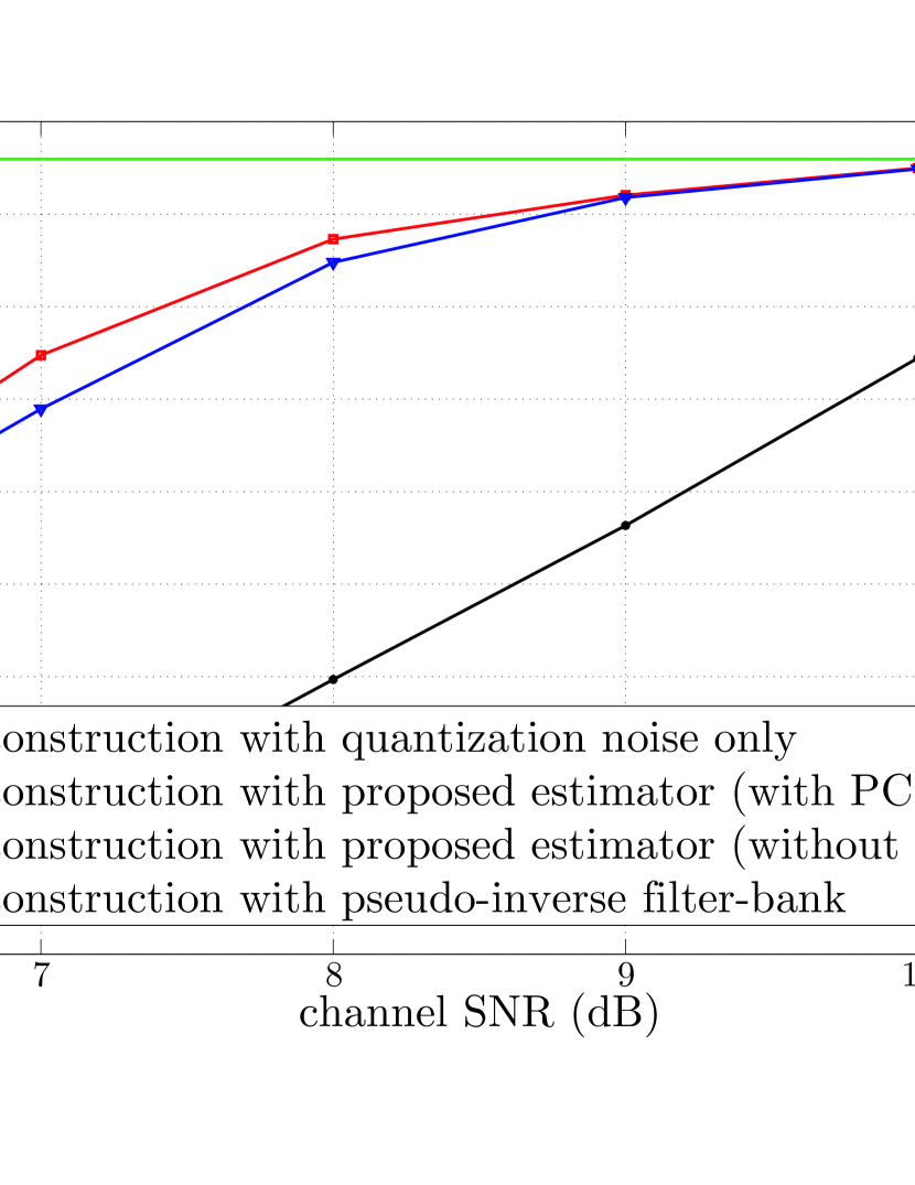
Figure 2: SNR of reconstructed signals as a function of channel SNR for Lines $55$ to $58$ of Lena.pgm

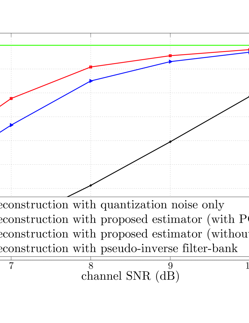
Figure 3: SNR of reconstructed signals as a function of channel SNR for correlated Gaussian signal

Figures 2 and 3 show the average reconstruction SNR as a function of the channel SNR. Three reconstruction methods are compared. The OFB input signal is reconstructed with the proposed estimator (with and without PCT) and with the conventional reconstruction method that uses the synthesis filter $R(z)$ on the most likely vector of indexes, after its inverse quantization, at each time instant, without paying any attention to the fact that it may not belong to $\mathcal{U}_{1}$. The number of candidates considered at each iteration has been set to $N_{\max}=20$. The reference reconstruction SNR corresponds to a signal corrupted only by quantization noise.

For both signals and without the use of the PCT, a gain of about $8$ dB in reconstruction SNR is observed for a channel SNR of $7$ dB and a gain of about $2.5$ dB in the channel SNR is observed for a signal SNR of $14$ dB . The use of the PCT in the proposed algorithm improves the performance in terms of reconstructed signal SNR. For a channel SNR level of $7$ dB, the gain in signal SNR is about $1$ dB for the first signal and of $2$ dB for the second one.

For the Gaussian correlated signal, the correlation between samples has not been explicitly taken into account here. It may be taken into account in (16) to further improve estimation performance.

7 Conclusion

In this paper we presented an estimation method that exploits the redundancy introduced by OFB as well as the fact that the noise introduced by the quantization operation is bounded.

The obtained experimental results have shown the improvement brought by this approach when compared to a classical estimation technique. The use of a parity-check filter bank allows to increase the performances of the method. This motivates us to propose methods that use the PCT in a more efficient way. Future work will be dedicated as well to extending the proposed approach to images and video.

References

• [1] C. E. Shannon, “A mathematical theory of communication,” Bell Syst. Tech. J., vol. 27, pp. 379–423, 1948.
• [2] P. Duhamel and M. Kieffer, Joint source-channel decoding: A cross-layer perspective with applications in video broadcasting, Academic Press, 2009.
• [3] A. K. Katsaggelos and F. Zhai, Joint Source-Channel Video Transmission, Morgan  Claypool, 2007.
• [4] H. Bölcskei and F. Hlawatsch, “Oversampled filterbanks: Optimal noise shaping, design freedom and noise analysis,” in Proc. IEEE Conf. on Acoust. Speech Signal Process., Munich, Germany, 1997, vol. 3, pp. 2453–2456.
• [5] Z. Cvetković and M. Vetterli, “Oversampled filter banks,” IEEE trans on Signal Processing, vol. 46, no. 5, pp. 1245–1255, 1998.
• [6] V. K. Goyal, M. Vetterli, and N. T. Thao, “Quantized overcomplete expansions in $\mathbb{R}^{n}$ : Analysis, synthesis, and algorithms,” IEEE Transactions on Information Theory, vol. 44, no. 1, pp. 16–31, 1998.
• [7] J. F. Kurose and K. W. Ross, Computer Networking: A Top-Down Approach Featuring the Internet, Addison Wesley, Boston, third edition, 2005.
• [8] J. Kovacević, P. L. Dragotti, and V. K Goyal, “Filter bank frame expansions with erasures,” IEEE trans. Information Theory, vol. 48, no. 6, pp. 1439 –1450, 2002.
• [9] G. Rath and C. Guillemot, “Frame-theoretic analysis of DFT codes with erasures,” IEEE trans. on Signal Processing, vol. 52, no. 2, pp. 447–460, 2004.
• [10] T. Petrisor, C. Tillier, B. Pesquet-Popescu, and J.-C. Pesquet, “Comparison of redundant wavelet schemes for multiple description coding of wavelet sequences,” in Proc. IEEE ICASSP, Philadelphia, PA, 2005, vol. 5 pp. 913-916.
• [11] M. Akbari and F. Labeau, “Recovering the output of an OFB in the case of instantaneous erasures in sub-band domain,” in Proc. MMSP, St Malo, France, 2010, pp. 274-279.
• [12] M. Ghosh, “Analysis of the effect of impulse noise on multicarrier and single carrier QAM systems,” IEEE trans. on Communication, vol. 44, no. 2, pp. 145–147, 1996.
• [13] F. Labeau, J.C. Chiang, M. Kieffer, P. Duhamel, L. Vandendorpe, and B. Mack, “Oversampled filter banks as error correcting codes: theory and impulse correction,” IEEE trans. on Signal Processing, vol. 53, no. 12, pp. 4619 – 4630, 2005.
• [14] G. R. Redinbo, “Decoding real-number convolutionnal codes: Change detection, Kalman estimation,” IEEE trans. on Information Theory, vol. 43, no. 6, pp. 1864–1876, 1997.
• [15] G. R. Redinbo, “Wavelet codes: Detection and correction using Kalman estimation,” IEEE trans. on Signal Processing, vol. 57, no. 4, pp. 1339–1350, 2009.
• [16] J. B. Anderson and S. Mohan, Source and Channel Coding: An Algorithmic Approach, Kluwer, 1991.
• [17] L. Jaulin, M. Kieffer, O. Didrit, and E. Walter, Applied Interval Analysis, Springer-Verlag, London, 2001.
• [18] P. P. Vaidyanathan, Multirate Systems and Filterbanks, Prentice-Hall, Englewood-Cliffs, NJ, 1993.
• [19] E. Walter and L. Pronzato, Identification of Parametric Models from Experimental Data, Springer-Verlag, London, 1997.