Sliding-Trellis based Frame Synchronization

Abstract

Frame Synchronization (FS) is required in several communication standards in order to recover the individual frames that have been aggregated in a burst. This paper proposes a low-delay and reduced-complexity Sliding Trellis (ST)-based FS technique, compared to our previously proposed trellis-based FS method. Each burst is divided into overlapping windows in which FS is performed. Useful information is propagated from one window to the next. The proposed method makes use of soft information provided by the channel, but also of all sources of redundancy present in the protocol stack. An illustration of our ST-based approach for the WiMAX Media Access Control (MAC) layer is provided. When FS is performed on bursts transmitted over Rayleigh fading channel, the ST-based approach reduces the FS latency and complexity at the cost of a very small performance degradation compared to our full complexity trellis-based FS and outperforms state-of-the-art FS techniques.

I Introduction

FS is an important problem arising at various layers of the protocol stack of several communication systems. The most obvious being, at Physical (PHY) layer, to recover the payload and the side information (headers, etc…) of PHY packets or frames. First results [1, 2] considered data streams in which regularly spaced fixed patterns or Synchronization Words (SW) are inserted to delimit fixed-length frames, as is the case, e.g., at the PHY layer of Digital Video Broadcasting - Handheld (DVB-H) for MPEG2 transport stream frames. Synchronization tools based on the maximization of the correlation between the SW and the received data have been proposed in [1]. This has been improved in [2], where the optimal statistic for FS has been proposed for the AWGN case, taking into account the presence of data around the SW. This was further extended in [3] for more sophisticated transmission schemes and in [4, 5] to provide robustness against frequency and phase errors.

In many communication systems, frames are of variable-length, see, e.g., the 802.11/802.16 standards [6, 7] for Wireless Local Area Networks (WLANs). In absence of SW, the Header Error Control (HEC) field of the header has been employed in [8] to perform FS with an automaton adapted from [9]. A length field, assumed present in the frame header, facilitates the FS when the noise is moderate. In [10, 11], several hypothesis testing techniques have been proposed to perform FS in presence of SW, which are further extended in [12] to exploit a priori information on the prevalence of ones and zeros in the payload at the price of a small additional signaling and computational complexity. However, insertion of SW requires some modification to the transmitter, which might not be standard compliant. Most of these FS techniques work on-the-fly, i.e., at each time, only few data samples are processed to perform FS and almost no latency is introduced.

Initially, FS has mainly been considered at PHY layer, albeit this problem may also occur at upper layers of the protocol stack. In fact, some frame aggregation techniques at intermediate protocol layers have been proposed recently in order to reduce the signalization overhead, see, e.g., [13] in the context of 802.11 standard. Efficient FS in this context is thus very important, since if some frames are not correctly delineated, a large amount of bits has to be retransmitted. In this context, processing a whole burst at each step may significantly improve the FS performance. This was evidenced in [14] for the segmentation of MAC frames aggregated in WiMAX PHY bursts, where Joint Protocol-Channel Decoding (JPCD) is performed using a modified BCJR algorithm [15] to obtain the frame boundaries. It exploits all available information: soft information at the output of the channel (or channel decoder) as well as the structure of the protocol layers (SW, known fields in headers, presence of Cyclic Redundancy Check (CRC) or checksums, etc).

This paper proposes an adaptation of the reduced-complexity Sliding Window (SW) [16] variant of the BCJR algorithm, presented for the decoding of convolutional codes, to develop a low-delay and reduced-complexity version of the FS technique presented in [14].

The FS problem is first stated as a maximum a posteriori (MAP) estimation problem in Section II. Then, Section III reformulates the trellis-based technique for FS introduced in [14]. The proposed ST-based algorithm is presented in Section IV and is illustrated in Section V with the FS of WiMAX MAC frames aggregated in bursts.

II MAP estimation for Frame Synchronization

II-A Frame structure

Consider the $n$-th variable-length frame at a given protocol layer. This frame is assumed to contain $\lambda_{n}=\ell_{h}+\ell_{p,n}$ bits, where the leading $\ell_{h}$ bits represent the frame header, of fixed length, and the remaining $\ell_{p,n}$ bits constitute the variable-length payload. In the header, $\ell_{c}$ bits are some HEC bits: CRC or checksum. The length $\lambda_{n}$ is assumed to be a realization of a stationary memoryless process $\Lambda$ characterized by

$$\pi_{\lambda}=\Pr\left(\Lambda=\lambda\right)\neq 0\text{ for }\ell_{\min}\leqslant\lambda\leqslant\ell_{\max},$$ (1)

where $\ell_{\min}$ and $\ell_{\max}$ are the minimum and maximum length in bits of a frame.

The header $\mathbf{h}_{n}$ of the $n$-th frame can be partitioned into four fields. The constant field $\mathbf{k}$, contains all bits which do not change from one frame to the next. It includes the SW indicating the beginning of the frame, and other bits which remain constant [17] once the communication is established. The header is assumed to contain a length field $\mathbf{u}_{n}$, indicating the size of the frame in bits $\lambda_{n}$, including the header. Our task is to estimate the successive values taken by this quantity in all frames of the burst. The other field $\mathbf{o}_{n}$, gathers all bits of the header which are not used to perform FS. Finally, the HEC field $\mathbf{c}_{n}$ is assumed to cover the $\ell_{h}-\ell_{c}$ ”working” bits of the header, i.e., $\mathbf{c}_{n}=\mathbf{f\left(\mathbf{k},\mathbf{u}_{n},\mathbf{o}\right)}$, where $\mathbf{f}$ is some (CRC or checksum) encoding function. The payload (assumed not protected by the HEC field) of the $n$-th frame is denoted by $\mathbf{p}_{n}$. It is modeled here as a binary symmetric sequence.

In what follows, the length of a vector $\mathbf{z}$ (in bits) is denoted as $\ell\left(\mathbf{z}\right)$ and its observation (soft information) provided either by a channel, a channel decoder, or a lower protocol layer is denoted as $\mathbf{y}_{z}$. $\mathbf{z}_{a}^{b}$ represents the sub-vector of $\mathbf{z}$ between indexes $a$ and $b$ (in bits).

II-B Aggregated frames within a burst

Consider a burst of $L$ bits consisting of $N$ aggregated frames. This burst contains either $N-1$ data frames and an additional padding frame containing only padding bits, or $N$ data frames. Assume that each of these frames, except the padding frame, contains a header and a payload and follows the same syntax, as described in Section II-A.

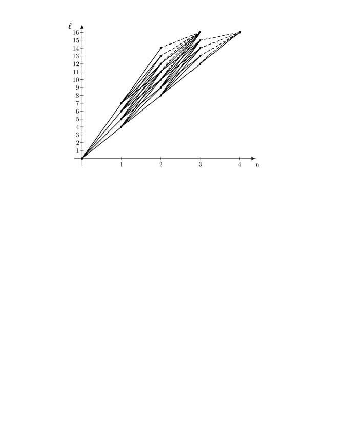
Figure 1: $L=16$ bits with $\ell_{\min}=4$ bits and $\ell_{\max}=7$ bits

Assuming that $L$ is fixed before frame aggregation and that $N$ is not determined a priori, the accumulated length in bits $\ell$ of the $n$ first aggregated frames can be described by a Markov process, which state is denoted by $S_{n}$. With this representation, the successive values taken by $S_{n}$, for $n=0,1,\dots$ can be described by a trellis [14] such as that of Figure 1, with a priori state transition probabilities $p\left(S_{n}=\ell\,|\,S_{n-1}=\ell^{\prime}\right)$ deduced from (1). If $\ell<L$, then

$$P\left(S_{n}=\ell\,|\,S_{n-1}=\ell^{\prime}\right)=\left\{\begin{array}[]{ll}\pi_{\ell-\ell^{\prime}}&\text{if }\ell_{\min}\leqslant\ell-\ell^{\prime}\leqslant\ell_{\max}\\ 0&\text{else,}\end{array}\right.$$ (2)

and if $\ell=L$, then

$$P\left(S_{n}=L\,|\,S_{n-1}=\ell^{\prime}\right) = \left\{\begin{array}[]{l}0\text{, if }L-\ell^{\prime}>\ell_{\max}\\ 1\text{, if }0<L-\ell^{\prime}<\ell_{\min}\\ \sum\limits_{k=L-\ell^{\prime}}^{\ell_{\max}}\pi_{k}\text{, else.}\end{array}\right.$$ (6)

In the trellis, dashed transitions correspond to padding frames and plain transitions correspond to data frames.

II-C Estimators for the number of frames and their boundaries

Consider a burst $\mathbf{x}_{1}^{L}$ of $N$ aggregated frames and some vector $\mathbf{y}_{1}^{L}$ containing soft information about the bits of $\mathbf{x}_{1}^{L}$. Here, one assumes that the first entry of $\mathbf{y}_{1}^{L}$ corresponds to the first bit of $\mathbf{x}_{1}^{L}$. This assumption is further discussed in Section III-C.

The suboptimal MAP estimator presented in [14] consists in first estimating $N$ and then in estimating the locations of the beginning and of the end of the frames. The MAP estimate $\widehat{N}_{\text{MAP}}$ of $N$ is given by

$$\widehat{N}_{\text{MAP}}=\arg\max_{N_{\min}\leqslant n\leqslant N_{\max}}P\left(S_{n}=L|\mathbf{y}_{1}^{L}\right),$$ (7)

with $N_{\min}=\left\lceil L/\ell_{\max}\right\rceil$, $N_{\max}=\left\lceil L/\ell_{\min}\right\rceil$, and $\left\lceil\cdot\right\rceil$ denoting the upward rounding. Once $\widehat{N}_{\text{MAP}}$ is obtained, the MAP estimate for the index $\ell_{n}$ of the last bit of the $n$-th $(n=1,...,\widehat{N}_{\text{MAP}})$ frame is

$$\widehat{\ell}_{n}=\arg\max_{\ell}P\left(S_{n}=\ell|\mathbf{y}_{1}^{L}\right),$$ (8)

and the length $\lambda_{n}$ of the $n$-th frame is estimated as

$$\widehat{\lambda}_{n}=\arg\max_{\ell}P\left(S_{n}=\ell|\mathbf{y}_{1}^{L}\right)-\arg\max_{\ell}P\left(S_{n-1}=\ell|\mathbf{y}_{1}^{L}\right).$$ (9)

III Trellis-based FS Algorithm

In $\eqref{Eq:MAPN},$ (8), and $\eqref{eq:MAPLambda}$, one has to evaluate $P(S_{n}=\ell|\mathbf{y}_{1}^{L})$ for all possible values of $n$ and $\ell$. This can be performed efficiently using the BCJR algorithm [15], by evaluating first

$$P(S_{n}=\ell,\mathbf{y}_{1}^{L})=\alpha_{n}\left(\ell\right)\beta_{n}\left(\ell\right)$$ (10)

where

$$\alpha_{n}(\ell)=P(S_{n}=\ell,\mathbf{y}_{1}^{\ell})=\sum_{\ell^{\prime}}\alpha_{n-1}(\ell^{\prime})\gamma_{n}(\ell^{\prime},\ell),$$ (11)

$$\beta_{n}(\ell)=P(\mathbf{y}_{\ell+1}^{L}|S_{n}=\ell)=\sum_{\ell^{\prime}}\beta_{n+1}(\ell^{\prime})\gamma_{n+1}(\ell,\ell^{\prime}),$$ (12)

and

$$\gamma_{n}\left(\ell^{\prime},\ell\right)=P(S_{n}=\ell,\mathbf{y}_{\ell^{\prime}+1}^{\ell}|S_{n-1}=\ell^{\prime}).$$ (13)

Classical BCJR forward and backward recursions allow to evaluate $\alpha$ and $\beta$. The initial value $S_{0}$ of the forward recursion is known, leading to $\alpha_{0}(\ell=0)=1$ and $\alpha_{0}(\ell\neq 0)=0$. For the backward recursion, assuming that all allowed final states are equally likely (which is a quite coarse approximation), one gets

$$\beta_{n}(L)=\frac{1}{N_{\max}-N_{\min}+1}\text{, }N_{\min}\leqslant n\leqslant N_{\max}\text{.}$$ (14)

All other values of $\beta_{n}(\ell)$, for $\ell<L$ are initialized to $0$.

III-A Evaluation of $\gamma_{n}$

Two cases have to be considered for evaluating $\gamma_{n}\left(\ell^{\prime},\ell\right)$.

When $\ell<L$, the transition corresponding to the $n$-th frame cannot be the last one, thus corresponds to a data frame. Assuming that $\ell_{\min}\leqslant\ell-\ell^{\prime}\leqslant\ell_{\max}$, the bits between $\ell^{\prime}+1$ and $\ell$ may be interpreted as $\mathbf{x}_{\ell^{\prime}+1}^{\ell}=\left[\mathbf{\mathbf{k}},\mathbf{\mathbf{u}}_{n},\mathbf{\mathbf{o}},\mathbf{\mathbf{c}},\mathbf{p}\right]$, where $\mathbf{\mathbf{u}}_{n}=\mathbf{u}\left(\ell-\ell^{\prime}\right)$ is the binary representation of $\ell-\ell^{\prime}$. The corresponding observation can be written as $\mathbf{y}_{\ell^{\prime}+1}^{\ell}=\left[\mathbf{y}_{k},\mathbf{y}_{u},\mathbf{y}_{o},\mathbf{y}_{c},\mathbf{y}_{p}\right]$. With these notations, for $\ell\neq L$, $\gamma_{n}\left(\ell^{\prime},\ell\right)=\gamma_{n}^{\text{d}}\left(\ell^{\prime},\ell\right)$, with

$$\gamma_{n}^{\text{d}}\left(\ell^{\prime},\ell\right) = p\left(S_{n}=\ell|S_{n-1}=\ell^{\prime}\right)\varphi^{\mathrm{d}}\left(\mathbf{y}_{\ell^{\prime}+1}^{\ell},\mathbf{x}_{\ell^{\prime}+1}^{\ell}\right),$$ (15)

where

$$\varphi^{\mathrm{d}}\left(\mathbf{y}_{\ell^{\prime}+1}^{\ell},\mathbf{x}_{\ell^{\prime}+1}^{\ell}\right) =P\left(\mathbf{y}_{k}|\mathbf{k}\right)P\left(\mathbf{y}_{u}|\mathbf{u}\left(\ell-\ell^{\prime}\right)\right)$$

$$\sum_{\mathbf{o}}P\left(\mathbf{y}_{o}|\mathbf{o}\right)P\left(\mathbf{y}_{c}|\mathbf{c=f}\left(\mathbf{k},\mathbf{u}\left(\ell-\ell^{\prime}\right),\mathbf{o}\right)\right)P\left(\mathbf{o}\right)$$

$$\sum_{\mathbf{p}}P\left(\mathbf{y}_{p}|\mathbf{p}\right)P\left(\mathbf{p}\right).$$ (16)

Under the assumptions described above and for a memoryless AWGN channel with variance $\sigma^{2}$, we get

$$P\left(\mathbf{y}_{u}|\mathbf{u}\left(\ell-\ell^{\prime}\right)\right)=P\left(\mathbf{y}_{u}|\mathbf{u}_{n}\right)=\prod_{i=1}^{\ell\left(\mathbf{u}_{n}\right)}\frac{1}{\sqrt{2\pi}\sigma}e^{-\left(\mathbf{y}_{u}(i)-\mathbf{u}_{n}(i)\right)^{2}/2\sigma^{2}}.$$

Assuming that the values taken by $\mathbf{p}$ are all equally likely, one gets $P\left(\mathbf{p}\right)=2^{-\ell\left(\mathbf{p}\right)}$.

In $\left(\ref{Eq:BigSumSimplified}\right)$, the sum over all possible $\mathbf{o}$ can be evaluated with a complexity $\mathcal{O}(\ell\left(\mathbf{o}\right)2^{\ell\left(\mathbf{c}\right)})$, as proposed in [17], see also [14] for more details.

When $\ell=L$ and $L-\ell^{\prime}<\ell_{\max}$, the $n$-th frame is the last one, and $\mathbf{x}_{\ell^{\prime}+1}^{L}=\mathbf{1}$ has also to be considered in $\gamma_{n}\left(\ell^{\prime},L\right)$, leading to

$$\gamma_{n}\left(\ell^{\prime},L\right) =\sum_{p=0,1}P(S_{n}=L,\mathbf{y}_{\ell^{\prime}+1}^{L},P_{n}=p|S_{n-1}=\ell^{\prime})$$

$$=\gamma_{n}^{\text{d}}\left(\ell^{\prime},L\right)P\left(P_{n}=0|S_{n-1}=\ell^{\prime}\right)$$

$$+\gamma_{n}^{\text{p}}\left(\ell^{\prime},L\right)P\left(P_{n}=1|S_{n-1}=\ell^{\prime}\right),$$ (17)

where $P_{n}$ is a random variable indicating whether the $n$-th frame is a padding frame and its a priori probability is given by

$$P\left(P_{n}=1|S_{n-1}=\ell^{\prime}\right) = \left\{\begin{array}[]{l}0\text{, if }L-\ell^{\prime}\geq\ell_{\max}\\ 1\text{, if }0<L-\ell^{\prime}<\ell_{\min}\\ \sum\limits_{\lambda=L-\ell^{\prime}+1}^{\ell_{\max}}\pi_{\lambda}\text{, else.}\end{array}\right.$$ (21)

In (17),

$$\gamma_{n}^{\text{p}}\left(\ell^{\prime},\ell\right) = P\left(S_{n}=L,\mathbf{y}_{\ell^{\prime}+1}^{L}|S_{n-1}=\ell^{\prime},P_{n}=1\right)$$ (22)

$$= P\left(\mathbf{y}_{\ell^{\prime}+1}^{L}|P_{n}=1,S_{n-1}=\ell^{\prime},S_{n}=\ell\right)$$

accounts for the padding frame, while

$$\gamma_{n}^{\text{d}}\left(\ell^{\prime},L\right) = P\left(S_{n}=L,\mathbf{y}_{\ell^{\prime}+1}^{\ell}|S_{n-1}=\ell^{\prime},P_{n}=0\right)$$

$$= P\left(S_{n}=L|S_{n-1}=\ell^{\prime},P_{n}=0\right)\varphi^{\mathrm{d}}\left(\mathbf{y}_{\ell^{\prime}+1}^{\ell},\mathbf{x}_{\ell^{\prime}+1}^{\ell}\right)$$

accounts for the data frame, with

$$P\left(S_{n}=L|S_{n-1}=\ell^{\prime},P_{n}=0\right)=\frac{\pi_{L-\ell^{\prime}}}{\sum\limits_{\lambda=\ell_{\min}}^{L-\ell^{\prime}}\pi_{\lambda}}.$$

III-B Complexity evaluation

The complexity of the FS algorithm described in Section II is proportional to the number of nodes or to the number of transitions within the trellis on which FS is performed. From Figure 1, one sees that the trellis is lower-bounded by the line $\ell=n\ell_{\min}$ and upper-bounded by the lines $\ell=n\ell_{\max}$ and $\ell=L$. This region may be divided into two triangular sub-regions, one with $0\leq n\leq N_{\min}-1$, bounded between $\ell=n\ell_{\min}$ and $\ell=n\ell_{\max}$, and the other with $N_{\min}\leq n\leq N_{\max}-1$, bounded between $\ell=n\ell_{\min}$ and $\ell=L$. Thus, summing up the number of nodes in each sub-region, one gets the number of nodes in the trellis

$$\mathcal{N}_{{\normalcolor n}} = \sum_{n=0}^{N_{\min}-1}n\left(\ell_{\max}-\ell_{\min}\right)+\sum_{n=N_{\min}}^{N_{\max}}\left(L-n\ell_{\min}\right).$$ (23)

Taking $N_{\min}\approx L/\ell_{\max}$ and $N_{\max}\approx L/\ell_{\min},$ (23) simplifies to

$$\mathcal{\mathcal{N}}_{\mathrm{n}}=\frac{L^{2}}{2}\left(\frac{\ell_{\max}-\ell_{\min}}{\ell_{\max}\ell_{\min}}\right)=\mathcal{O}\left(L^{2}\right).$$ (24)

From each node, at most $\ell_{\max}-\ell_{\min}$ transitions may emerge. Thus, from $\left(\ref{eq:Nodes}\right)$, the number of transitions $\mathcal{\mathcal{N}}_{\mathrm{t}}$ may also approximated as $\mathcal{\mathcal{N}}_{\mathrm{t}}=\mathcal{O}\left(L^{2}\right).$

III-C Limitations

The hold-and-sync technique presented in [14] for performing FS is based on the knowledge of the beginning and length of the burst. This requires an error-free decoding of the headers of lower protocol layers, which contain this information. This may be done using methods presented in [17], which enable the lower layer to forward the burst to the layer where it is processed. The main drawback of this FS technique in terms of implementation is the increase in memory requirements for storing soft information. This is estimated in [18, 19] to be three to four times more. However, the plain trellis-based FS algorithm, as described above, requires buffering the whole burst which induces some buffering and processing delays proportional to $L^{2}$, see (24). To alleviate these problems, a new low-delay and less-complex variant of the previously presented FS technique is now proposed.

IV Sliding Trellis-based FS

In classical SW-BCJR methods, decoding is done within a window, which at each step is shifted bit-by-bit [16] or by several bits [20]. From one window to the next, the results obtained during the forward iteration are reused, contrary to those of the backward iteration. The number of bits the window is shifted at each iteration determines the trade-off between complexity and efficiency.

Contrary to the trellis for a convolutional code, the trellis considered in Figure 1 has a variable number of states for each value of the frame index $n$. One may apply directly the SW ideas, but due to the increase of the size of the trellis (at least for small values of $n$), this would still need very large trellises to be manipulated, with an increased computation time. Here, a ST-based approach is introduced: a reduced-size trellis is considered in each decoding window. As in [20], some overlapping between windows is considered, in order to allow better reuse of already computed quantities and to allow complexity-efficiency trade-offs.

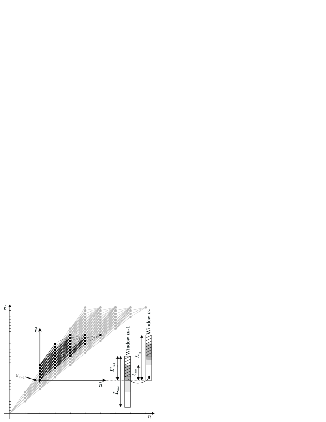
Figure 2: ST for the $m$-th decoding window, the original trellis is in gray

IV-A Sliding Trellis

In the proposed ST-based approach, a burst of $L$ bits is divided into $M$ overlapping windows with sizes $L_{m}$, $m=1,...,M$. For each of these windows, the bits from $\varepsilon_{m-1}+1$ to $\varepsilon_{m-1}+L_{m}$ are considered, where $\varepsilon_{m-1}$ is the bit index of the last bit of the last frame deemed reliably synchronized in the $m-1$-th window.

A ST moves from window to window to perform decoding. One such ST is illustrated in Figure 2. Let $\bar{n}$ and $\bar{\ell}$ be the local trellis coordinates. Once $P(S_{\bar{n}}^{m}=\bar{\ell}|\mathbf{y}_{\varepsilon_{m-1}+1}^{\varepsilon_{m-1}+L_{m}})$ is evaluated, one can apply the estimators (7), (8), and (9) to determine the number of frames $\widehat{N}_{m}$ in the $m$-th window (including the last truncated frame), the beginning, and the length of each frame. For the $m$-th window ($m<M$), among the $\widehat{N}_{m}$ decoded frames, only the first $\widehat{N}_{m}^{c}$ frames are considered as reliably synchronized, since enough data and redundancy properties have been taken into account. Truncated frames, especially when the HEC has been truncated, and the frame immediately preceding such frames, are not considered reliable. Thus, only the $\widehat{N}_{m}^{c}$ complete frames ending in the first $L_{m}-\ell_{\max}-\ell_{h}$ bits of the window are considered as reliable. The unreliable region towards the boundary of the window is dashed in Figure 2.

The initialization of $\beta$ is performed as in Section III, since no knowledge from the previous window can be exploited. The initialization of $\alpha$ and the evaluation of $\gamma$ towards the window boundary may depend on the location of the window inside a burst. Three types of window locations are considered: the first window at the start of a burst, the intermediate windows in the middle of the burst, and the last window at the end of the burst.

The first window ($m=1$) contains $L_{m}<L$ bits and starts at $\varepsilon_{0}=0$. The decoding approach, including the initialization of $\alpha$ for this first window is similar to that presented for the trellis-based approach. An exception is the computation of $\gamma_{\bar{n}}\left(\bar{\ell}^{\prime},\bar{\ell}\right)$, where two cases have again to be considered. The first corresponds to normal data frames, leading to $\gamma_{\bar{n}}^{\text{d}}\left(\bar{\ell}^{\prime},L_{m}\right)$. The second accounts for truncated data frames towards the boundary of the window, leading to $\gamma_{\bar{n}}^{\text{t}}\left(\bar{\ell}^{\prime},L_{m}\right)$, which is detailed in Section IV-B.

The intermediate windows ($1<m<M$) contain the bits from $\varepsilon_{m-1}+1$ to $\varepsilon_{m-1}+L_{m}<L$, see Figure 2. The bit index $\varepsilon_{m-1}$, of the last bit of the last frame deemed reliably synchronized (i.e., the $\widehat{N}_{m-1}^{c}$-th frame) in the $m-1$-th window, corresponds in the local coordinates of the $m-1$-th ST to $\bar{\ell}=\varepsilon_{m-1}-\varepsilon_{m-2}$. The $m$-th ST starts at the local coordinates $(\bar{n}=\widehat{N}_{m-1}^{c},\bar{\ell}=\varepsilon_{m-1}-\varepsilon_{m-2})$ of $m-1$-th ST. The computation of $\gamma_{\bar{n}}\left(\bar{\ell}^{\prime},\bar{\ell}\right)$ for an intermediate window is identical to that of the first window. For the initialization of $\alpha_{\bar{n}}^{m}\left(\bar{\ell}\right)$, following the idea of the SW-BCJR decoder [21, 16], up to $\ell_{\max}$ initial values for $\alpha_{0}^{m}\left(\bar{\ell}\right)$ are propagated from the $m-1$-th window to the $m$-th window, see Section IV-C. This allows a better FS in case of erroneous FS in the $m-1$-th window.

The last window ($m=M$) has no incomplete frame at its end. Only the presence of a padding frame has to be taken into consideration. The decoding is performed as in the trellis-based approach (Section III), except for the initialization of $\alpha_{0}^{M}\left(\bar{\ell}\right)$, which is similar to that of the intermediate window case.

Note that the $m$-th and $m+1$-th windows overlap over $L_{m}^{o}$ bits, with $\ell_{h}+\ell_{\max}\leqslant L_{m}^{o}<\ell_{h}+2\ell_{\max}$.

IV-B Evaluation of $\gamma_{\bar{n}}$

When $m<M,$ transitions corresponding to truncated frames have to be considered at the end of the window. When the size of the truncated frame is larger than $\ell_{h}$, the header is entirely contained in the truncated frame. In this case $\gamma_{\bar{n}}\left(\bar{\ell}^{\prime},L_{m}\right)=\gamma_{\bar{n}}^{\mathrm{t}}\left(\bar{\ell}^{\prime},L_{m}\right),$ with

$$\gamma_{\bar{n}}^{\mathrm{t}}\left(\bar{\ell}^{\prime},L_{m}\right)=p\left(S_{\bar{n}}^{m}=L_{m}|S_{\bar{n}-1}^{m}=\bar{\ell}^{\prime}\right)\varphi^{\mathrm{t}}\left(\mathbf{y}_{\bar{\ell}^{\prime}+1}^{L_{m}},\mathbf{x}_{\bar{\ell}^{\prime}+1}^{L_{m}}\right).$$ (25)

In (25), since truncated frames have to be considered, $p\left(S_{\bar{n}}^{m}=L_{m}|S_{\bar{n}-1}^{m}=\bar{\ell}^{\prime}\right)$ is given by (6). Moreover, the length of the frame, i.e., the content of the length field $\mathbf{\mathbf{u}}_{n}$, is now only known to be between $\max(L_{m}-\bar{\ell}^{\prime},\ell_{\min})$ and $\ell_{\max}$ bits. Thus

$$\varphi^{\mathrm{t}}\left(\mathbf{y}_{\bar{\ell}^{\prime}+1}^{L_{m}},\mathbf{x}_{\bar{\ell}^{\prime}+1}^{L_{m}}\right) =P\left(\mathbf{y}_{k}|\mathbf{k}\right)\sum_{\mathbf{p}}P\left(\mathbf{y}_{p}|\mathbf{p}\right)P\left(\mathbf{p}\right)$$

$$\sum_{\ell=\max(L_{m}-\bar{\ell}^{\prime},\ell_{\min})}^{\ell=\ell_{\max}} \vspace{-10mm}P\left(\mathbf{\mathbf{u}\left(\ell\right)}\right)\sum_{\mathbf{o}}\left(P\left(\mathbf{y}_{u}|\mathbf{u}\left(\ell\right)\right)P\left(\mathbf{y}_{o}|\mathbf{o}\right)\right.$$

$$\left.P\left(\mathbf{y}_{c}|\mathbf{c=f}\left(\mathbf{k},\mathbf{u}\left(\ell\right),\mathbf{o}\right)\right)P\left(\mathbf{o}\right)\right).$$ (26)

When the size of the truncated frame is strictly less than $\ell_{h}$, for the sake of simplicity, we assume that all bits of the truncated header are equally likely. In such case $\gamma_{\bar{n}}\left(\bar{\ell}^{\prime},L_{m}\right)=\gamma_{\bar{n}}^{\text{e}}\left(\bar{\ell}^{\prime},L_{m}\right),$ with

$$\gamma_{\bar{n}}^{\mathrm{e}}\left(\bar{\ell}^{\prime},L_{m}\right) = p\left(S_{\bar{n}}^{m}=L_{m}|S_{\bar{n}-1}^{m}=\bar{\ell}^{\prime}\right)$$ (27)

$$\sum_{\mathbf{x}_{\bar{\ell}^{\prime}+1}^{L_{m}}}P\left(\mathbf{y}_{\bar{\ell}^{\prime}+1}^{L_{m}}|\mathbf{x}_{\bar{\ell}^{\prime}+1}^{L_{m}}\right)P\left(\mathbf{x}_{\bar{\ell}^{\prime}+1}^{L_{m}}\right),$$

where $p\left(S_{\bar{n}}^{m}=L_{m}|S_{\bar{n}-1}^{m}=\bar{\ell}^{\prime}\right)$ is still given by (6) and $P(\mathbf{x}_{\bar{\ell}^{\prime}+1}^{L_{m}})=2^{-\ell(\mathbf{x}_{\bar{\ell}^{\prime}+1}^{L_{m}})},$ since all beginning of headers are assumed equally likely.

For $m=M,$ the evaluation of $\gamma_{\bar{n}}^{M}$ is as in Section III-A.

IV-C Initialization of $\alpha$ in the sliding trellises

In the SW-BCJR algorithm proposed in [16], the $\alpha^{m}$s evaluated in the $m$-th window are deduced from those evaluated in the $m-1$-th window. Here, since the number of states $S_{n}$ evolves with $n$, $\alpha_{\bar{n}}^{m}$ cannot be obtained that easily from $\alpha_{\bar{n}}^{m-1}$.

In the $m-1$-th window, one has evaluated $\alpha_{\bar{n}}^{m-1}\left(\bar{\ell}\right)$, with $0\leqslant\bar{\ell}\leqslant L_{m-1}$ and $0\leqslant\bar{n}\leqslant\left\lceil L_{m-1}/\ell_{\min}\right\rceil$. We choose to propagate at most $\ell_{\max}$ values of $\alpha$ from $\bar{n}=\widehat{N}_{m-1}^{c}$ in the $m-1$-th window to $\bar{n}=0$ in the $m$-th window (for $\bar{\ell}=0,...,\ell_{\max}-1$) as follows

$$\alpha_{0}^{m}(\bar{\ell})=\kappa\,\alpha_{\widehat{N}_{m-1}^{c}}^{m-1}\left(\varepsilon_{m-1}-\varepsilon_{m-2}+\bar{\ell}\right),$$ (28)

where $\kappa$ is some normalization factor chosen such that the $\alpha_{0}^{m}(\bar{\ell})$s sum to one. This allows the first frame of the $m$-th window to start at any bit index between $\varepsilon_{m-1}+1$ and $\varepsilon_{m-1}+\ell_{\max}$.

IV-D Complexity

Consider $M$ windows of approximately the same size $L^{w}$, which are overlapping on average on $L^{o}=\ell_{h}+1.5\ell_{\max}$ bits. For sufficiently large $L$, one has to process $M\approx\frac{L}{L^{w}-L^{o}}$ overlapping windows, each one with

$$\mathcal{\mathcal{N}}_{\mathrm{n}}^{w}\approx\frac{\left(L^{w}\right)^{2}}{2}\left(\frac{\ell_{\max}-\ell_{\min}}{\ell_{\max}\ell_{\min}}\right)$$

nodes. The total number of nodes to process is then

$$M\mathcal{\mathcal{N}}_{\mathrm{n}}^{w}\approx\frac{L}{L^{w}-L^{o}}\frac{\left(L^{w}\right)^{2}}{2}\left(\frac{\ell_{\max}-\ell_{\min}}{\ell_{\max}\ell_{\min}}\right).$$ (29)

This decoding complexity is smaller than that of Section III-B. A comparison for different values of burst size $L$ is provided in Table I for window size $L^{w}=480+L^{o}$. One can observe that the complexity gain increases with the size of the burst.

$L$ (bytes)	1800	8000	16000	24000
Trellis-based (# of Nodes)	24300	480000	1920000	4320000
ST-based (# of Nodes)	17400	77200	154450	231700
Complexity Gain	1.4	6.2	12.5	18.6

TABLE I: FS Complexity Comparison for $L^{w}=480+L^{o}$

Choosing small values for $L^{w}$ reduces the latency as well as the complexity at the cost of some sub-optimality in the decoding performance. Note that $L^{w}$ cannot be chosen too small (smaller than $\ell_{h}+2\ell_{\max}$) to ensure at least one reliable FS in each window.

V Simulation results

In the WiMAX standard [7], the downlink (DL) sub-frames are divided into bursts. Each burst can contain multiple concatenated fixed-size or variable-size MAC frames: it is filled with several MAC frames, until there is not enough space left. Padding bytes (0xFF) are then added [7] at the end of the burst. Each MAC frame begins with a fixed-length header, followed by a variable-length payload and ends with an optional CRC. As we are considering only the DL case, where the connection is already established, MAC frames belonging to a burst contain only Convergence Sublayer (CS) data, so only the Generic MAC header [7] is possible inside a burst.

Some assumptions are made in what follows for the sake of simplicity. CRC, ARQ, packing, fragmentation, and encryption are not used for the MAC frames inside the burst. Some fields are already fixed in a MAC header, and with the considered situation, fields such as Header Type (HT), Encryption Control (EC), sub-headers and special payload types (Type), Reserved (Rsv), CRC Indicator (CI), and Encryption Key Sequence (EKS) remain constant. The LEN field, representing the length in bytes of the MAC frame, and the Connection IDentifier (CID) have variable contents. The Header Check Sequence (HCS), an 8-bit CRC, is used to detect errors in the header and is a function of the content of all header fields.

The considered simulator consists of a burst generator, a BPSK modulator, a channel, and a receiver. Simulations are carried over Rayleigh fading channels, where the modulated signal is subject to zero mean and unit variance fast (bit) Rayleigh fading plus zero-mean AWGN noise. For performance analysis, Erroneous Frame Location Rate (EFLR) is evaluated as a function of the channel Signal-to-Noise Ratio (SNR). It should be noted that in order to recover a frame correctly both ends of the frame have to be correctly determined.

In our simulations, $L=1800$ bytes. Since WiMAX MAC frames are byte-aligned, i.e., the LEN field of the frame is in bytes and all MAC frames contain an integer number of bytes, $\alpha$, $\beta$, and $\gamma$ are evaluated for $\ell$s corresponding to the beginning of bytes. Data frames are randomly generated with a length uniformly distributed between $\ell_{\min}=50$ bytes and $\ell_{\max}=200$ bytes. If there is not enough space remaining in the burst, a padding frame is inserted to fill the burst. The burst is then BPSK modulated and sent over the channel.

Simulation results for the trellis-based FS technique (Section II), the ST-based approach (Section IV), a FS based on hard decision on the received bits, and a state-of-the-art on-the-fly technique (denoted by MU, for modified Ueda’s method) described in [8] are shown in Figure 3. MU technique involves a three-state automaton for FS and uses the HCS as an error-correcting code. Here, the method in [8] has been modified to cope with short (8-bit) HCS, where several candidates for two-bit error syndromes are possible.

For the ST-based approach, the burst is divided into three windows, with $L_{1}=600$ bytes, $L_{2}=600+L_{1}^{o}$ bytes, and $L_{3}=600+L_{2}^{o}$ bytes. Compared to the trellis-based FS, the ST-based approach shows a slight performance degradation of $0.5$ dB, but reduces the delay and the computational complexity. On average, the overlap is about $277$ bytes and a decrease in complexity by a factor of 1.7 is observed. The computational complexity of the on-the-fly MU technique is much smaller than that of the ST-based approach, at the cost of a noticeable loss in efficiency.

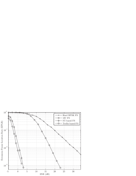
Figure 3: FS methods for transmission over Rayleigh channel

VI Conclusion

A reduced-complexity, low-delay, and efficient ST-based technique for the robust FS of aggregated frames is presented. Compared to the trellis-based FS algorithm proposed in [14], the FS delay and computational complexity are significantly reduced. The price to be paid is a slight performance degradation.

This technique has been applied to the FS of WiMAX MAC bursts. A significant gain in performance is obtained for Rayleigh fading channels compared to classical FS. Extensions to perform on-the-fly FS, by utilizing the features of Ueda’s method and at the same time exploiting the structural properties of the headers of frames, are currently under investigation.

References

- [1] R. H. Barker, Group synchronization of binary digital systems in Communication Theory., W. Jackson, Ed. Butterworth, London, 1953.
- [2] J. L. Massey, “Optimum frame synchronization,” IEEE Trans. on Comm., vol. 20, no. 4, pp. 115–119, 1972.
- [3] G. L. Lui and H. H. Tan, “Frame synchronization for Gaussian channels,” IEEE Trans. on Comm., vol. 35, no. 8, pp. 818–829, 1987.
- [4] Z. Y. Choi and Y. H. Lee, “Frame synchronization in the presence of frequency offset,” IEEE Trans. Comm., vol. 50, pp. 1062–1065, 2002.
- [5] D.-U. Lee, P. Kim, and W. Sung, “Robust frame synchronization for low signal-to-noise ratio channels using energy-corrected differential correlation,” EURASIP J. Wirel. Commun. Netw., vol. 2009, pp. 1–8.
- [6] IEEE802.11n Part 11: Wireless LAN Medium Access Control (MAC) and Physical layer (PHY) specifications: Enhancements for Higher Throughput, IEEE Std., March 2006.
- [7] ANSI/IEEE, “802.16: IEEE standard for local and metropolitan area networks, air interface for fixed broadband wireless access systems,” Tech. Rep., 2004.
- [8] U. Ueda, H. Yamaguchi and R. Watanabe, “Reducing misframe frequency for HEC-based variable length frame suitable for IP services,” in Proc. IEEE ICC 2001, 2001, pp. 1196 – 1200.
- [9] B - ISDN user-network interface - Physical layer specification: General characteristics, ITU-T Std., 1999.
- [10] M. Chiani and M. G. Martini, “On sequential frame synchronization in AWGN channels,” IEEE Trans. Comm., vol. 54, pp. 339 – 348, 2006.
- [11] M. G. Martini and M. Chiani, “Optimum metric for frame synchronization with Gaussian noise and unequally distributed data symbols,” in Proc. IEEE SPAWC, Perugia, Italy, 21-24 June 2009.
- [12] M. G. Martini and C. Hewage, “Cross-layer frame synchronization for H.264 video over WiMAX,” in Proc. IEEE SPAWC, Marrakech, Morocco, June 2010.
- [13] A. Sidelnikov, J. Yu, and S. Choi, “Fragmentation/aggregation scheme for throughput enhancement of IEEE 802.11n WLAN,” in proc. IEEE APWCS, 2006.
- [14] U. Ali, M. Kieffer, and P. Duhamel, “Joint protocol-channel decoding for robust aggregated packet recovery at WiMAX MAC layer.” in Proc. IEEE SPAWC, Perugia, Italy, 21-24 June 2009, pp. 672 – 676.
- [15] L. R. Bahl, J. Cocke, F. Jelinek, and J. Raviv, “Optimal decoding of linear codes for minimizing symbol error rate,” IEEE Trans. Info. Theory, vol. 20, pp. 284–287, 1974.
- [16] S. Benedetto, D. Divsalar, G. Montorsi, and F. Pollara, “Soft-output decoding algorithms for continuous decoding of parallel concatenated convolutional codes,” in proc. ICC, Dallas, TX, 1996, pp. 112 – 117.
- [17] C. Marin, Y. Leprovost, M. Kieffer, and P. Duhamel, “Robust header recovery based enhanced permeable protocol layer mechanism,” in Proc. IEEE SPAWC, 2008, pp. 91–95.
- [18] G. Panza, E. Balatti, G. Vavassori, C. Lamy-Bergot, and F. Sidoti, “Supporting network transparency in 4G networks,” in Proc. IST Mobile and Wireless Communication Summit, 2005.
- [19] R. G. Woo, P. Kheradpour, D. Shen, and D. Katabi, “Beyond the bits: cooperative packet recovery using physical layer information,” in Proc, ACM MobiCom, 2007, pp. 147 – 158.
- [20] J. Gwak, S. K. Shin, and H. M. Kim, “Reduced complexity sliding window BCJR decoding algorithms for turbo codes,” in IMA - Crypto & Coding’99, M. Walker, Ed. Springer-Verlag, 1999, pp. 179–184.
- [21] S. Benedetto, D. Divsalar, G. Montorsi, and F. Pollara, “Algorithm for continuous decoding of turbo codes,” Electronics Letters, vol. 32, no. 4, pp. 314 – 315, 1996.