Cosmological parameter estimation using Particle Swarm Optimization (PSO)

Abstract

Constraining theoretical models, which are represented by a set of parameters, using observational data is an important exercise in cosmology. In Bayesian framework this is done by finding the probability distribution of parameters which best fits to the observational data using sampling based methods like Markov Chain Monte Carlo (MCMC). It has been argued that MCMC may not be the best option in certain problems in which the target function (likelihood) posses local maxima or have very high dimensionality. Apart from this, there may be examples in which we are mainly interested to find the point in the parameter space at which the probability distribution has the largest value. In this situation the problem of parameter estimation becomes an optimization problem. In the present work we show that Particle Swarm Optimization (PSO), which is an artificial intelligence inspired population based search procedure, can also be used for cosmological parameter estimation. Using PSO we were able to recover the best fit LCDM parameters from the WMAP seven year data without using any prior guess value or any other property of the probability distribution of parameters like standard deviation, as is common in MCMC. We also report the results of an exercise in which we consider a binned primordial power spectrum (to increase the dimensionality of problem) and find that a power spectrum with features gives lower chi square than the standard power law. Since PSO does not sample the likelihood surface in a fair way, we follow a fitting procedure to find the spread of likelihood function around the best fit point.

I Introduction

In a typical CMB data analysis pipeline first the time order data, obtained from an instrument like WMAP, is reduced into a set of sky maps from which angular power spectra are computed, and finally these spectra are reduced into a set of cosmological parameters representing a model usually using Bayesian analysis  1996PhRvD..54.1332J ; 1996PhRvL..76.1007J ; 2002PhRvD..66j3511L ; 2002PhRvD..66f3007K ; 2003ApJS..148..195V ; 2010LNP…800..147V ; 2003moco.book…..D ; 2011ApJS..192…14J ; 2011ApJS..192…16L ; 2003moco.book…..D . The exercise of parameter estimation involves identifying a set of parameters which has the highest probability of giving the observed data i.e., finding a point in the multidimensional parameter space at which the likelihood function has the greatest value. Currently this exercise is done using some sampling based methods, like MCMC, in which the likelihood function is sampled at discrete points, which are further used to compute various statistics of parameters  2001CQGra..18.2677C ; 2002PhRvD..66j3511L ; 2010LNP…800..147V . Apart from MCMC, non-sampling based methods inspired from artificial intelligence techniques, like artificial neural network, have also been successfully applied in cosmological parameter estimation from the CMB data 2007MNRAS.376L..11A .

In the present work we demonstrate the use of another artificial intelligence inspired method, named Particle Swarm Optimization or PSO KennedEberhart1995 ; KennedEberhart2001 ; Engelbrech2002 , for cosmological parameter estimation using WMAP seven year datalambda . Being a stochastic method, PSO also has the interesting feature that the computational cost for searching the global maximum in the multi-dimensional space does not grow exponentially with the dimensionality of the search space. However, in this case also (like other stochastic methods) the probability of convergence to the global maximum is usually guaranteed only in the asymptotic limit. Based on a very simple idea and having very few design parameters, PSO is quite easy to program and can provide accurate results very fast. As compared to artificial neural network 2007MNRAS.376L..11A all the calculations in PSO are exact, in the sense that no extrapolation or interpolation is done at any stage i.e., fitness function is computed exactly at all points. It has been found that PSO can outperform MCMC in certain situations, in particular when there are a large number of local maxima present and/or the dimensionality of the search space is very high 2010PhRvD..81f3002W .

It has been a common practice to consider a featureless primordial power spectrum (PPS), characterized by two parameters tilt ($n_{s}$) and amplitude ($A_{s})$. In this case also there is a degeneracy between the parameters of PPS and other cosmological parameters (like $\Omega_{b}$), but the likelihood surface remains fairly smooth and does not poses much challenge for the MCMC method. There have been studies which show that a PPS with features is a better fit to the observational data as compared to the featureless power law PPS 2010JCAP…10..008H ; 2011arXiv1106.2798A ; 2011arXiv1109.5264M . In one of such studies 2011arXiv1109.5264M a PPS with oscillations is considered and it is argued that due to additional degrees of freedom, as a result of features, the MCMC approach is not very successful since there are a large number of local maxima present in the search space and the chains frequently tunnel from one local maximum to another. In order to circumvent this problem it has been recommended first to carry out the search space over a subset of parameters over a grid and then use full MCMC. PSO can be quite useful in this type of problem due to its better capabilities of handling higher dimensional search space and large number of local maxima.

Since the fitness function i.e., the function to be optimized, can be computed concurrently on a parallel platform for a large number of particles, PSO promises to give accurate results very fast, if implemented efficiently.

Unlike MCMC which provides the full probability distribution from which marginalized values of parameters and error bars can be computed, PSO just gives the location of the best fit point, called the Gbest, (definition in next section) and one needs to find some way to compute error bars. In the present work we fit the effective chi square ($\chi^{2}_{\rm{eff}}=-2\log{\mathcal{L}}$) by a multi-dimensional paraboloid around the best fit point and compute the error bars from the fitting coefficients of that. On the basis of the errors we set the range for the two dimensional grids which we consider for various combinations of parameters (keeping all other parameters fixed to their best fit values) and make contour plots which show not only the extent to which the likelihood surface is spread (errors) but also the correlation between various parameters. These contour plots also confirm that PSO does find the global maximum of the likelihood function.

We observe that in most cases (which we have considered) not only does the Gbest  approach towards the best fit point, the average location of particles also approaches towards it, as PSO progresses. The average location of PSO particles in the multi-dimensional search space can be used to check the robustness of PSO. Since PSO is designed mainly for finding the best fit point, therefore the sampling done by PSO particles is not designed to be a fair representation of the likelihood surface.

The plan of the paper is as follows. In § II we discuss a simple implementation of the Particle Swarm Optimization in detail. In particular, we focus on the dynamics of particles, setting-up initial conditions, boundary conditions and the convergence criteria. We also define all the design parameters and variables of PSO in § II. A very brief overview of parameter estimation in Bayesian formalism is discussed in  §III. In place of discussing the full prescription of Maximum Likelihood (ML) estimation, we mainly focus on the computation of error bars from covariance or Hessian matrix in this section. We present our results of parameter estimation using PSO for WMAP seven year data in § IV. Apart from giving the best fit parameters and errors which we get from our fitting exercise, we also present contour plots for various combinations of the parameters. Along with the best fit parameter estimates which we get from PSO, we give a comparison of the results obtained from PSO and as are reported by WMAP team using MCMC. In §V we summarize the PSO and discuss its advantages and disadvantages.

II Particle Swarm Optimization

Formally proposed by James Kennedy and Russell Eberhart in 1995 KennedEberhart1995 , PSO has been successfully tested and applied in many engineering and artificial intelligence problems Lazinic2009 ; Boeringer2004 ; Robinson2004 . Recently it has been applied in astrophysical problems also 2005MNRAS.359..251S ; 2010PhRvD..81f3002W ; 2011ApJ…727…80R . In PSO, a set of “particles” driven by “cognition” and “social” factors explore the multi-dimensional search space by carrying out random walks, determined by a set of “design parameters”. The accuracy and performance of the algorithm depends on the values of the design parameters as well as the function to be optimized i.e., the fitness function.

Particle Swarm Optimization is based on observations of social dynamics, bird flocks, fish schools and other forms of group behavior. Personal discoveries made by members of the group and shared with everyone else can help everyone to become more efficient in making new discoveries. Efficient personal search and communication with other members of the group can lead to rapid success for the group in search of some common goal i.e., food etc.

At present there exists many implementations of the Particle Swarm Optimization. Here we consider one of the simplest forms KennedEberhart1995 the elements of which are shared by many other implementations. Before describing the working of our PSO implementation, it is useful to define some of the key terms which are used to describe PSO.

1. Particles:- The term “particles” in PSO is used for “computational agents” and has no relation with any form of physical particles. PSO particles have no mass and occupy no volume (however, they can have weights called inertia weights which will be discussed later). PSO particles are distinguished from each other on the basis of their identification numbers or  ids and have “positions” and “velocities”. In our discussion we represent the position and velocity of a particle with id   i at step (“time”) $t$ by vector $X^{i}(t)$ and $V^{i}(t)$ respectively.

2. Fitness function:- The function ${\mathcal{F}}(X)$ to be used for searching the global maximum is called the “fitness function” or “optimization function”. In the present case we use $-2\log{\mathcal{L}}$ or $\chi^{2}_{\rm{eff}}$ as our optimization function, where ${\mathcal{L}}$ is the CMB likelihood function.

3. Pbest:- The maximum value of the optimization function ${\mathcal{F}}^{i}(t)$ for a particle $i$ till the present step (time $N_{t}$) is called its $\text{{Pbest}}^{i}$.

   $$\text{{Pbest}}^{i}=\text{Max}\{{\mathcal{F}}^{i}(t),t=0,1,2...,N_{t}\}$$ (1)

   the location of the $\text{{Pbest}}^{i}$ is represented by the vector $P^{i}$

   $$P^{i}=X^{i}(t)~{}~{}\text{if}~{}~{}{\mathcal{F}}^{i}(t)=\text{{Pbest}}^{i}$$ (2)

4. Gbest:- The largest value of Pbest  among all particles is called the   Gbest. The value of Gbest  changes only when any of the particles finds a new position at which the value of the fitness function is larger than any of the earlier values.

   $$\text{{Gbest}}=\text{Max}\{\text{{Pbest}}^{i},i=0,1,2...,N_{p}\}.$$ (3)

   Here $N_{p}$ is the number of particles. The location of the  Gbest  is given by the vector $G$.

   $$G=X^{i}(t)~{}~{}\text{if}~{}~{}\text{{Pbest}}^{i}=\text{{Gbest}}.$$ (4)

II.1 Dynamics of PSO particles

The following equation is used to update the positions of the particles KennedEberhart1995 ,

$$X^{i}(t+1)=X^{i}(t)+V^{i}(t+1),$$ (5)

where velocity $V^{i}(t+1)$ for the particle $i$ at step $(t+1)$ is computed in the following way

$$V^{i}(t+1)=wV^{i}(t)+c_{1}\xi_{1}\left\{X^{i}(t)-P^{i}\right\}$$

$$+c_{2}\xi_{2}\left\{X^{i}(t)-G\right\}.$$ (6)

Here $c_{1}$ and $c_{2}$ are called acceleration coefficients, $w$ is called the inertia weight and $\xi_{1}$ and $\xi_{2}$ are two uniform random numbers in the range $[0,1]$. The values of the acceleration coefficients $c_{1}$ and $c_{2}$ decide the contribution due to personal (cognitive) learning and social learning respectively.

The first factor in the right hand side of equation  (6) moves the particle along a straight line and the second and third factors accelerate it towards the location of  Pbest  and  Gbest  respectively. Kennedy and Eberhart KennedEberhart1995 use $c_{1}=c_{2}=2$ to give it a mean of unity, so that the particle would overfly the target about half of the time.

Although the equation (6) is most commonly used, the following version is also in use 2005MNRAS.359..251S .

$$V^{i}(t+1)=K\left\{V^{i}(t)+C_{1}\xi_{1}\left(X^{i}(t)-P^{i}\right)\right.$$

$$\left.+C_{2}\xi_{2}\left(X^{i}(t)-G\right)\right\}$$ (7)

where $K$ is called the constriction factor and is defined in the following way:

$$K=\frac{2}{|2-\phi-\sqrt{\phi^{2}-4\phi}|}$$ (8)

where $\phi=C_{1}+C_{2}$. Here the recommended values are $C_{1}=C_{2}=2.05$ which gives $K=0.729$. Equation (7) is equivalent to equation  (6) with $c_{1}=KC_{1},c_{2}=KC_{2}$ and $w=K$. Since there are many implementations (with different values of design parameters or with some new parameters) we have decided to work with PSO standard 2006 pso2006 which uses the following values of the design parameters in equation (6)

$$w=\frac{1}{2\log(2)}=0.72$$ (9)

and

$$c_{1}=c_{2}=0.5+\log(2)=1.193$$ (10)

since we were able to get quite accurate results with the values of design parameters suggested in PSO standard 2006pso2006 , we decided to adopt these values in our implementation. We did try a few other values but could not find any significant improvement.

In particle swarm optimization all the particles can communicate with each other or the communication can be restricted between only subsets of particles. The first case is found to be more useful for intensive local search and the second one for global search. In our implementation we let every particle share the information about its  Pbest  with every other particle.

II.2 Maximum Velocity

In order to stop particles leaving the search space we need to limit the maximum velocity which particles can acquire. This can be done by setting the maximum velocity along various dimensions. It has been a common practice to keep the maximum velocity proportional to the search range.

$$V^{i}(t)=\begin{cases}V_{max},&\text{if}~{}~{}V^{i}(t)>V_{max}\\ -V_{max},&\text{if}~{}~{}V^{i}(t)<-V_{max}\end{cases}$$ (11)

where $V_{max}$ is also a design parameter. We use $V_{max}=c_{v}(X_{max}-X_{min})$ with $c_{v}=0.5$ where $[X_{min},X_{max}]$ is our search range. This means that the biggest jump a particle can make is half of the size of the search range.

II.3 Initial Conditions

We assign random positions and velocities to particles in the beginning.

$$X^{i}(t=0)=X_{min}+\xi\times(X_{max}-X_{min})$$ (12)

and

$$V^{i}(t=0)=\xi V_{max},$$ (13)

where $\xi$ is a uniform random number in the range $[0-1]$. Apart from the above initial conditions “particles on a grid” initial condition can also be used. From our trial runs we have found that the final outcome i.e., the location of the Gbest  is not very sensitive to the initial condition.

II.4 Boundary condition

We use the “reflecting wall” boundary condition in which a particle reverses its velocity component perpendicular to the boundary when it tries to cross the boundary.

$$V^{i}(t)=-V^{i}(t)$$ (14)

and

$$\begin{cases}X^{i}(t)=X_{max}&\text{when}~{}~{}X^{i}(t)>X_{max}\\ X^{i}(t)=X_{min}&\text{when}~{}~{}X^{i}(t)<X_{min}\end{cases}$$ (15)

II.5 Termination criteria

PSO particle trajectories are like “chains” in MCMC, however, they are coupled to each other by second acceleration coefficient $c_{2}$. In the limit of $c_{2}=0$ particle do not exchange information but in that case PSO will become meaningless. We have used Gelman-Rubin R statistics1992GelmanRubin ; 1998BrooksGelman in order to find out when the exploration by PSO particles should be stopped. In order to use Gelman-Rubin statistics we use the mean of variance $W$ within PSO particle trajectories and variance of the mean $B$ across PSO trajectories.

At any time $N_{t}$ the mean value the trajectory of a PSO particle is

$${\bar{X}}^{i}=\sum\limits_{j=1}^{N_{t}}X^{i}(t)$$ (16)

and the variance

$$\sigma^{2}_{i}=\frac{1}{N_{t}-1}\sum\limits_{j=1}^{N_{t}}(X^{i}(t)-{\bar{X}}^{i})^{2}$$ (17)

and the mean of variance

$$W=\frac{1}{N_{p}}\sum\limits_{i=1}^{N_{p}}\sigma_{i}^{2}$$ (18)

In order to compute variance of means we firstly compute mean of means

$$Y=\sum\limits_{i=1}^{N_{p}}{\bar{X}}^{i}$$ (19)

and then

$$B=\frac{N_{t}}{N_{p}-1}\sum\limits_{i=1}^{N_{p}}({\bar{X}}_{i}-Y)^{2}$$ (20)

The variance of stationary distribution can be written as weighted sum of $W$ and $B$.

$$Z=\left(1-\frac{1}{N_{t}}\right)W+\frac{1}{N_{t}}B$$ (21)

The potential scale reduction factor ${\hat{R}}$ is given by

$${\hat{R}}=\sqrt{\frac{Z}{W}}$$ (22)

In general when the value of ${\hat{R}}$ as low as 1 we can assume that the convergence has been obtained.

Parameter	Description	Value
$w$	Inertia weight	0.72
$c_{1}$	Acceleration parameters (personal)	1.193
$c_{1}$	Acceleration parameters (social)	1.193
$c_{v}=V_{max}/\Delta X$	maximum velocity parameter	0.5
$N_{p}$	Number of particles	30
$N_{d}$	Search dimensions	6

Table 1: PSO design parameters

III Cosmological Parameter estimation

Cosmic Microwave Background temperature and polarization anisotropies observed in the sky represent the fluctuations in the baryon-photon fluid at the epoch of last scattering i.e., when electrons were last scattered by photons before they combined with protons and formed hydrogen atoms, contain a lot of information about the cosmological parameters 1984ApJ…285L..45B ; 2004astro.ph..3344C ; 1996LNP…470..207H ; 2003moco.book…..D . Due to the Gaussian nature of the density fluctuations at the epoch of last scattering (primordial fluctuations) as predicted by inflationary models, the most important information about the cosmological parameters is encoded in the angular two point correlation function or power spectrum.

It is a common practice to represent the temperature anisotropies in the CMB sky in spherical harmonic expansion

$$\frac{\Delta T({\hat{n}})}{T_{0}}=\sum\limits_{lm}a_{lm}Y_{lm}({\hat{n}})$$ (23)

where $T_{0}$ is the average temperature i.e., the monopole term. The angular two point correlation function is given by

$$C(\theta)=\left<\frac{\Delta T({\hat{n}})}{T_{0}}\frac{\Delta T({\hat{n}}^{\prime})}{T_{0}}\right>=\sum\limits_{l}\frac{2l+1}{4\pi}C_{l}P_{l}{\cos\theta}$$ (24)

where $\theta$ is angle between directions ${\hat{n}}$ and ${\hat{n}^{\prime}}$ in the sky. The angular power spectrum $C_{l}$ is defined as

$$C_{l}=\left<a_{lm}a^{*}_{lm}\right>=\left<|a_{lm}|^{2}\right>.$$ (25)

As mentioned above, the angular power spectrum $C_{l}$ (or angular two point correlation function $C(\theta)$) depends on a large number of cosmological parameters representing various energy densities in the universe, primordial fluctuations, and the physical processes relevant in the early universe like reionization and recombination 1984ApJ…285L..45B ; 1987MNRAS.226..655B ; 1997MNRAS.291L..33B ; 1998PhRvD..57.2117B . Many of the cosmological parameters affect the angular power spectrum in the same way, i.e., have degeneracies. However, it is possible to form a set of parameters, called “normal parameters” which affect the angular power spectrum in a unique way 2003ApJ…596..725C ; 1997MNRAS.291L..33B . The most common cosmological parameters which have been used to fit observational $C_{l}$ (we also use these) are density parameters for cold dark matter ($\Omega_{c}h^{2}$), baryons $(\Omega_{b}H^{2})$, cosmological constant $(\Omega_{\Lambda})$, primordial scalar power spectrum index $(n_{s})$, and normalization $(A_{s})$, and reionization optical depth $(\tau)$. In our analysis we do not consider the “Hubble parameter” $h$ as a free parameter and compute its value from other parameters for a spatially flat model.

$$h=\sqrt{\frac{\Omega_{b}h^{2}+\Omega_{c}h^{2}}{1-\Omega_{\Lambda}}}$$ (26)

It is now a common practice to follow a “ line of sight ” integration approach for computing the angular power spectrum $C_{l}$ for a set of cosmological parameters which is a computationally expensive process. The publicly available code CAMB  camb ; 2000ApJ…538..473L is based on an earlier code named CMBFAST  1996ApJ…469..437S which can compute the angular power spectrum $C_{l}$ on a shared memory platform in a short time.

III.1 Bayesian Analysis

In the framework of Bayesian analysis the probability of obtaining a set of parameters $\Theta$ which is consistent with a data set $D$ for a given prior $I$ is given by

$$P(\Theta|D,I)=\frac{P(D|\Theta,I)P(\Theta|I)}{P(D|I)}.$$ (27)

In the above equation $P(\Theta|D,I)$ is the posterior probability distribution, $P(D|\Theta,I)$ is the likelihood function (which will be represented by ${\mathcal{L}}$) and $P(\Theta|I)$ is the prior. The denominator $P(D|I)$ called “evidence” is used for the purpose of normalization and does not depend on the parameters $\Theta$ so it can be ignored for the present purpose.

The likelihood function for a CMB experiment with $N_{p}$ pixels is given by 2003moco.book…..D

$${\mathcal{L}}(\Delta|\Theta)=\frac{1}{(2\pi)^{N_{p}/2}}\frac{1}{|C|^{N_{p}/2}}\exp\left[-\frac{1}{2}\Delta C^{-1}\Delta\right]$$ (28)

where  $\Delta$  represents an estimator of the observed data vector, having $N_{p}$ entries, and $C$ is the joint covariance matrix i.e., sum of the signal and noise covariance matrix

$$C=S+N.$$ (29)

The noise covariance matrix $N$ can be approximated by a diagonal matrix and the signal covariance matrix $S$ is given by 2010LNP…800..147V

$$S_{ij}=\sum\limits_{l}\frac{2l+1}{4\pi}C_{l}P_{l}(\cos\theta)$$ (30)

where $\theta$ is the angle between the directions ${\hat{n}}_{i}$ and ${\hat{n}}_{j}$ representing pixel $i$ and pixel $j$ respectively.

Exact likelihood computation by a brute force method is computationally expensive since it involves inversion of a $N_{p}\times N_{p}$ matrix which is a formidable task for an experiment with very large number of pixels. Many approximations have been proposed which reduce the cost of likelihood computation significantly 2008PhRvD..77j3013H ; 2009PhRvD..79h3012H ; 2010LNP…800..147V .

In the present work we use the likelihood code provided by the WMAP team for computing the likelihood function, which takes the theoretical angular power spectrum computed by CAMB, and the power spectrum estimated by the WMAP experimentwmap , as inputs.

The exercise of obtaining the best fit cosmological parameters involves finding a point in the multidimensional parameter space, at which the value of the likelihood function ${\mathcal{L}}$ is maximum or $-2\log{\mathcal{L}}$ is minimum. Apart from the best fit values one is also interested in the error bars on the estimated parameters which involves knowing the shape of the likelihood function around the best fit values, for which we follow a fitting procedure as discussed below.

III.2 Likelihood fitting

Close to the best fit point we can approximate the likelihood function Gaussian :

$${\mathcal{L}}={\mathcal{L}}_{0}\exp[-\frac{1}{2}\Delta^{T}R\Delta]$$ (31)

where $\Delta_{i}=\theta_{i}-\theta_{i,0}$ where $\theta_{i,0}$ is the maximum likelihood value of the parameter $\theta_{i}$ and $R$ is the curvature matrix. The covariance matrix $C$ which is the inverse of curvature matrix $R$ gives an estimate of the standard errors which maximum likelihood fitting can give 1996PhRvD..54.1332J .

The standard error $\Delta\theta_{i}$ in parameter $\theta_{i}$ is given by:

$$\Delta\theta_{i}=\sqrt{C_{ii}}=1/\sqrt{[(R)^{-1}]_{ii}}$$ (32)

We fit $-2(\log{\mathcal{L}}-\log{\mathcal{L}}_{0})=\Delta\chi^{2}_{\rm{eff}}$ with a paraboloid and compute the coefficients of fitting and identify those with the elements of curvature matrix.

IV Results

We compute the best fit cosmological parameters from the WMAP seven year data for a six parameter model with model parameters $\Omega_{b}h^{2},\Omega_{c}h^{2},\Omega_{\Lambda},n_{s},A_{s}$ and $\tau$ using PSO. Before presenting our results quantitatively, we consider it useful to present a qualitative comparison of the way parameters are estimated in the Markov-Chain Monte Carlo methods and in Particle Swarm Optimization. In particular, we want to highlight the way parameter space is explored and sampled in PSO and MCMC methods.

IV.1 Markov Chain and PSO exploration

Figure 1: In this figure the red line shows a Markov chain which has been obtained from a typical run of COSMOMC and the green line shows the trajectory of a PSO particle, along the same dimension i.e. $\Omega_{b}h^{2}$. Markov chain as well as a PSO trajectory can begin anywhere in the range and progressively move towards the best fit location. However, in the case of PSO the particle approaches towards the best fit location (Gbest) in an oscillatory manor with successively decreasing amplitude, which is not the case for a Markov Chain since its step size does not vary much. Only after a sufficient number of PSO steps the particle positions and the Markov chain converge. Since there are more number of points for the Markov chain as compared to the PSO, we use x-scale such that we have five Markov points for every PSO point.

The nature of exploration by a Markov chain and that by a set of PSO particles is completely different. However, there are some similarities also, for example, in both the cases the random walk is governed by the optimization function or the fitness function. In MCMC, the proposal density is directly related to the function to be sampled. In the case of MCMC exploration of a chain is completely local, in the sense that whether a step will be selected or rejected depends only on the values of the fitness function at the current location and the next location. However, in the case of PSO, particles always have some information about the global maximum  Gbest , which keeps changing. In general the step size does not change in MCMC, however, in the case of PSO it rapidly falls as  Gbest  approaches close to the global maximum.

Figure 2: In this figure the red and the green points show the distribution of the positions of PSO particles and samples from a Markov chain respectively, in the same plane. From the figure it can be noticed that in the initial stage the scatter of PSO particles is very large (see Figure 1 also), however, close to the convergence all particles get confined in a very compact region. The distribution of the sample points in the case of Markov chain is much more symmetric than in PSO. We suspect that this is due to the different role played by the stochastic variables (random numbers) in PSO as compared to that in the Markov chains. The non-symmetric distribution makes PSO less favorable if we want to find the shape of the likelihood close to the best fit values (in order to report errors) in comparison to Markov Chain.

Markov chains sample the fitness function in the multi-dimensional parameter space using methods like Metropolis Hastings. The sampling algorithm ensures that more points are sampled from regions in which the fitness function has large values and less points from the regions in which it has small values. The values of best fit parameters are obtained after marginalization. In case of PSO a set of “particles” explore the multidimensional space guided by their personal i.e., Pbest  and collective i.e., Gbest  discoveries (see equation (5) and equation (6)). The progress of a chain in MCMC and trajectory of a particle in PSO are very different. Starting from any arbitrary point in the multi-dimensional space both approach towards the region where the probability of global maximum is high, however, the way they approach is different.

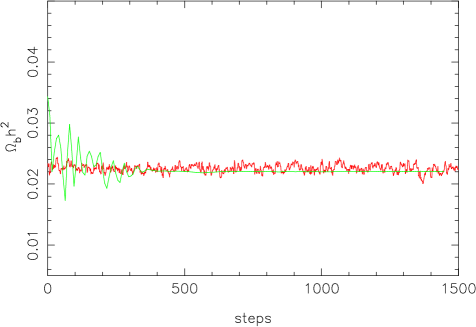
Figure 1 shows a typical Markov chain and the trajectory of a PSO particle. Since there were greater number of steps in the Markov chain than in PSO, we have stretched the x-axis for PSO trajectory by a factor of five, i.e, there are five Markov chain points for every PSO point for the same range on the x-axis. From the figure it can be noticed that the PSO particle reaches the global maximum by performing oscillatory motion with gradually decreasing amplitude. However, in the case of Markov chain the progress is very smooth.

One of the most common ways to present the results of a parameter estimation exercise is to make two dimensional scatter or contour plots. In MCMC it is done by marginalizing the sampled function along all other dimensions apart from the two for which we want scatter or contour plots. For a general case, the location of the point at which the likelihood function peaks may be different from the average location computed on the basis of the one dimensional probability distribution obtained after marginalization. In the case of PSO also, we present the average location of the particles, apart from finding the point at which the likelihood function peaks.

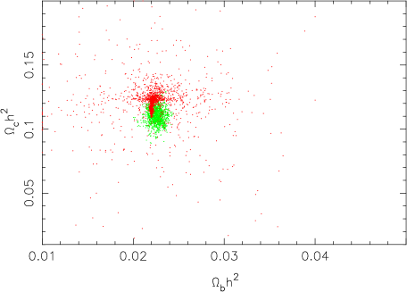
The red and green points in Figure 2 show the projection of the positions of PSO particles and a set of sample points from a Markov chain in a two-dimensional plane of the parameter space, respectively. From the figure it can be noticed that although the sampled points in both cases cluster around the same point (Gbest  in PSO) the distribution are completely different. In particular the points are more symmetrically distributed around the best fit value in the Markov chain case as compared to that in PSO. Since PSO results are always quoted in term of  Gbest  therefore the distribution of points does not change the results in any way. However, since in the present work we make explicit use of the PSO particle distribution also (for fitting the likelihood function for computing errors), it can create some problem.

IV.2 Best fit cosmological parameters

Figure 3: The solid line in the above figure shows the change in the fitness function $-2\log{\mathcal{L}}$ as PSO steps progress, and the dashed line shows the value for the WMAP seven year data. From this figure it can be noticed that in the beginning improvement in the value of the fitness function is quite rapid, but after some time it saturates, primarily because once the particles reach close to the global maximum as given by the Gbest  their velocities drop.

In order to test the working of our PSO module we considered a six dimensional cosmological model $(\Omega_{b}h^{2},\Omega_{c}h^{2},\Omega_{\Lambda},n_{s},A_{s},\tau)$ (see Figures 1 of 2011ApJS..192…16L ) and tried to estimate its parameters from the WMAP seven year data. The range over which we tried to optimize our fitness function and the results are given in Table (2).

Cosmological parameters from PSO
Variable		PSO best fit			WMAP best fit2011ApJS..192…16L		Difference (Gbest-ML)
	Range	Gbest($\chi^{2}_{\rm{eff}}=7469.73$)	Mean	std dev.	ML($\chi^{2}_{\rm{eff}}=7486.57$)	Mean
$\Omega_{b}h^{2}$	(0.01,0.04)	0.022036	0.022030	0.000456	0.02227	$0.02249^{0.00056}_{-0.00057}$	-0.000234(-1.05%)
$\Omega_{c}h^{2}$	(0.01,0.20)	0.112313	0.112435	0.005276	0.1116	$0.1120\pm 0.0056$	0.000713 (0.63%)
$\Omega_{\Lambda}$	(0.50,0.75)	0.721896	0.720353	0.029047	0.729	$0.727^{+0.030}_{-0.029}$	-0.007104(-0.97%)
$n_{s}$	(0.50,1.50)	0.963512	0.963278	0.011730	0.966	$0.967\pm 0.014$	-0.002488(-0.25%)
$A_{s}/10^{-9}$	(1.0,4.0)	2.448498	2.454202	0.106615	2.42	$2.43\pm 0.11$	0.028498(1.17%)
$\tau$	(0.01,0.11)	0.08009	0.083930	0.012113	0.0865	$0.088\pm 0.015$	-0.00641(-7.41%)

Table 2: The first column in the above table shows the PSO fitting parameters and the second, third, fourth and fifth columns show the search range, the location of  Gbest, the average position of PSO particles and the error (which is computed by fitting the sampled function) respectively. In the sixth and seventh columns we give the best fit (ML) and the average values of the cosmological parameters derived from WMAP seven years likelihood estimation respectively. In the last column we give the difference between our best fit parameters (PSO parameters) and WMAP team’s best fit parameters (difference between ML and Gbest  values). From this table it is clear that roughly there is good agreement between the PSO best fit parameters and WMAP team’s best fit parameters from the seven year data.

In Figure 3 we show the evolution of the fitness function ($-2\log{\mathcal{L}}$) with PSO steps. We also show value for the fitness function for WMAP seven years best fit cosmological parameters (dashed line). From the figure it can be noticed that the value obtained by PSO finally converges to the WMAP seven year value. Since the velocity with which particles move toward  Gbest  is proportional to their distance from  Gbest, we get large jumps in the fitness function in the beginning.

Figure 4: In each panel of the above figure we show the location of the best fit points (location of Gbest) and the average location of PSO particles, by the solid and dot-dashed lines respectively. We also show the best fit values given by the WMAP team by dashed lines. From the above figure it can be noticed that as PSO progresses the average location of PSO particles and the location of the Gbest  converge, which can be used as a robust check. For most cases the best fit values obtained by PSO match well with standard LCDM values, but there are some differences also (see table 2).

In PSO the values of the best fit parameters, location in the parameter space at which the likelihood function peaks, is represented by  Gbest. For consistency and robustness we not only give the location of the  Gbest, we also give the average location of the PSO particles. It is not a surprise that as PSO progresses, the average position of PSO particles and the location of the best fit point converge to Gbest. In a case when there are local maxima also present, some of the PSO particles may trap in these, but, the average location of particles still follows  Gbest. In Figure 4 we show the location of Gbest  and the average position of the PSO particles in our six dimensional search space at different steps. Note that in our model $h$ is not a fitting parameter, we get its value from the flatness condition (see equation (26)).

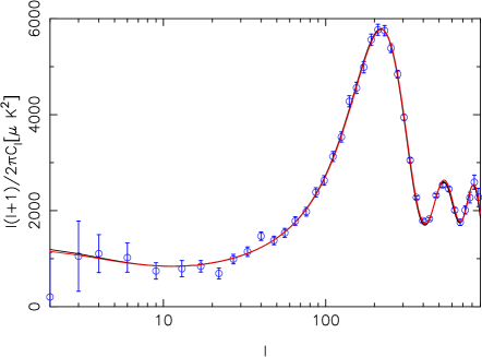
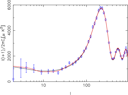
The black, red and blue lines in Figure 5 show the best fit angular power spectrum obtained by MCMC analysis, from PSO code and the binned power spectrum (with error bars) provided by the WMAP team for the seven year data. From the figure it is clear that the power spectrum which we obtain from our PSO code closely follows other two curves.

Figure 5: The red, black and blue lines in the above figure represent the best fit angular power spectrum recovered from PSO, standard LCDM power spectrum and the binned power spectrum of WMAP seven year data respectively. Note that the PSO best fit angular power spectrum is very close to that provided by the WMAP team. The small difference (see table (2)) between the PSO best fit parameters and the WMAP best fit parameters leads to a difference of 7 in $\chi^{2}_{\rm{eff}}$ (it is smaller by 7 for PSO).

IV.3 Error estimates

In order to compute error bars on the parameters estimated using PSO, we fit (as discussed in § III.2) a six dimensional paraboloid to a subset of sampled points to $\Delta\chi^{2}_{\rm{eff}}=-2\log{\mathcal{L}}-(-2\log{\mathcal{L}}_{0})$ where ${\mathcal{L}_{0}}$ is the value of the likelihood function or Gbestat the last PSO step.

$$\Delta\chi^{2}_{\rm{eff}}=[{\tilde{\Theta}}][\alpha][{\tilde{\Theta}}]^{T}$$ (33)

where $\Theta=(\Omega_{b}h^{2},\Omega_{c}h^{2},\Omega_{\Lambda},n_{s},A_{s},\tau)$ and $[\alpha]$ is a $6\times 6$ symmetric matrix with 21 independent coefficients.

The six dimensional vector ${\tilde{\Theta}}$ is defined as

$${\tilde{\Theta}}=\frac{\Theta-\Theta_{\texttt{Gbest}}}{\Theta_{\texttt{Gbest}}}.$$ (34)

We used multi-parameter fitting subroutine of GNU scientific library for the fitting gsl . In order to limit our fitting to a subset of points, we consider only those points which are within a six dimensional hyper-sphere of radius i.e., $|{\tilde{\theta}_{i}}|<0.1$ where $\theta_{i}$ is a component of the vector ${\tilde{\Theta}}$, and $\Delta\chi^{2}_{\rm{eff}}<10$.

After obtaining the fitting matrix $[\alpha]$ we invert it and compute the covariance matrix $[C]=[\alpha]^{-1}$ and compute error for the parameter $\theta_{i}$ from it

$$\Delta\theta_{i}=\sqrt{C_{ii}}\times\theta_{i,\texttt{Gbest}}.$$ (35)

We present the error in various parameters in the fifth column of Table (2).

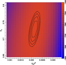
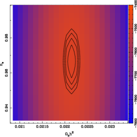
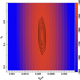
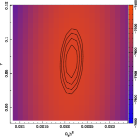
IV.4 Two dimensional contour plots

Figure 6: Panels in this figure show the two dimensional contour plots for various pairs of the six cosmological parameters $\Omega_{b}h^{2},\Omega_{c}h^{2},\Omega_{\Lambda},n_{s},A_{S}$ and $\tau$. We have considered a grid of size $24\times 24$ for our exercise considered the $3\sigma$ region, (where $\sigma$ is the error computed from the fitting) around the best fit point. In the case when we do not have any idea about the $\sigma$ we can give any other trial value also. The contours in the figure (from inside) are for $\Delta\chi^{2}=2,4,6,8$ and 10. Note that the contour plots not only give an idea about the area around the best fit region, they also clearly demonstrate correlation between various cosmological parameter.

Figure 7: Same as in Figure 6 but for different combination of cosmological parameters.

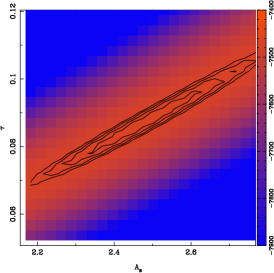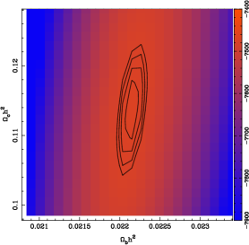
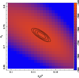
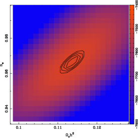
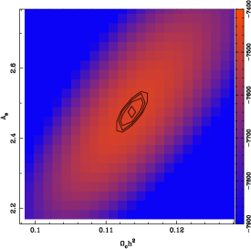
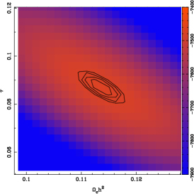
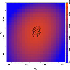
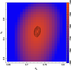
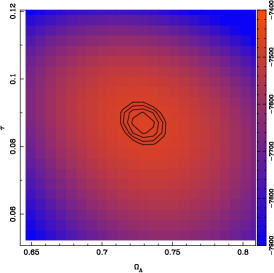
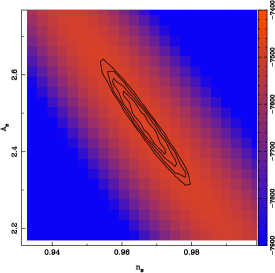
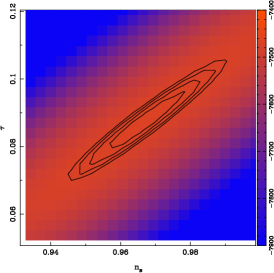
Fitting as we have done may not give a very good estimate of the errors on parameters. The exact way to figure out how the likelihood surface behaves around the best fit location, which is given by Gbest  in our case is to compute the likelihood function on a grid around the best fit point. Numerical computation over a multi-dimensional grid is quite expensive and even for a moderate size grid of 24 we have to do $24^{6}$ computations for a six parameter cosmological model. In place of considering a multi-dimensional grid we consider, $N_{d}(N_{d}-1)/2$ two dimensional grid as is done by some other authors 2003ApJ…596..725C . We fix the values of the four parameters out of six to their best fit values i.e., Gbest  and draw the two dimensional grid over the other two parameters.

In Figure 6 and 7 we show two dimensional contour plots for different pairs of cosmological parameters. The contours from the innermost are for $\Delta\chi^{2}=2,6,8$ and $10$. Note that the range for grids is selected from the rough estimates of errors which we get from fitting. The range for $\Omega_{c}h^{2}$ and $\Omega_{\Lambda}$ is taken $2\sigma$ and for others it is taken $3\sigma$ where $\sigma$ is the error obtained from the fitting

IV.5 Primordial Power Spectrum (PPS) with power in bins

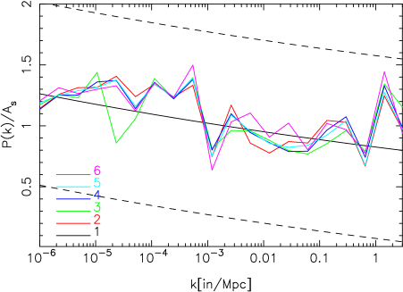
In order to demonstrate an interesting example in which PSO can be useful, we consider a model in which the primordial power spectrum has “binned” power in place of being a power law. We consider the power in bins as free parameters and that make our model higher dimensional. Apart from having 20 free parameters, which gives power in logarithmic bins we consider rest of the four parameters $\Omega_{b}h^{2},\Omega_{c}h^{2},\Omega_{\Lambda}$ and $\tau$ also free. As is expected, a model with more parameters better fits the observational data, which in the present case is WMAP seven year data i.e., for a primordial power spectrum with binned power $\chi^{2}$ is lower by 7 as compared to the standard power law mode. The best fit primordial power spectrum and angular power spectrum are shown in Figure 8 and Figure 9 respectively. Note that the PPS with binned power gives better fit, particularly at low l. We consider here the particular form of PPS not to motivate any particular theoretical model but just to demonstrate the method we use.

Figure 8: This figure shows how the binned primordial power spectrum (20 logarithmic bins over the $k$ range) changes as PSO progresses (line 1 is for the initial PPS and 6 is for the final PPS). The lower and upper values of the power in bins are represented by the dashed line. Starting with a power law PPS we found that a power spectrum which has low power in some bins and high in others fits better than a power law model.

Figure 9: The red, black and blue lines in the above figure represent the best fit angular power spectrum recovered from PSO, standard LCDM power spectrum and the binned power spectrum of WMAP seven year data respectively. Note that at low $l$ the angular power spectrum with binned PPS fits better as compared to the standard power law PPS to the observed data (the improvement in $\Delta\chi^{2}$ is around 7).

IV.6 Computational performance

Computing the fitness function i.e., $-2\log~{}{\mathcal{L}}$, which is the most expensive part in the parameter estimation procedure, involves two steps. In the first step the $C_{l}$s are computed for a set of cosmological parameters for which we use the publicly available code CAMB 2000ApJ…538..473L which employs OpenMP pragmas for doing computationally intensive steps in parallel on multi-processor shared memory systems. In the second step the likelihood function is computed from $C_{l}$s and the observational data i.e., WMAP seven year data, for which we use the likelihood code provided by the WMAP team. Since our PSO code shares two main modules ($C_{l}$ and likelihood computation) with the publicly available code COSMOMC, the difference in the performance is expected only due to the number of times the fitness function is computed. Computationally a typical PSO run gives very good convergence with 30 PSO particles with 160 steps i.e., 4800 computations. We ran a typical COSMOMC run with 24 chains and found that (from reading .log file for every chain) that CAMB was called 691200 times, which is more than 50 times the number of CAMB calls made in our case (including the calls for two dimensional grids used for contours).

Here it is also important to mention that parallelizing our code is very straightforward. We use OpenMP to compute $C_{l}$ for a point in the six dimensional parameter space and use MPI to distribute particles among different MPI nodes. At every step, particles are distributed among MPI nodes and after they return the value of the fitness function, the master node computes  Pbest  and  Gbest  and updates the positions and velocities of particles. We have tested our code on a Linux cluster using 15 MPI nodes, where each node has 2 AMD quad core Opetron 2.6 GHz processors. Within a node we use OpenMP for computing the angular power spectrum using as many number of threads as the number of cores are present. We have also ported our code on a Cray CX1 system with six nodes, where each node has 2 Intel Xeon 2.67 Ghz 6 core processors. In a case when the number of nodes can divide the number of PSO particles, there is no difficulty with load balance. Since at every PSO step a very small amount of data has to be communicated among MPI nodes, we have found that MPI collective communications calls like “broadcast” and “gather” are much more efficient than regular “send” and “receive” calls. In the present run, the result of which are reported here, it took roughly two and half hours for the standard PSO run to finish on a Linux cluster with 10 nodes with each node having 2 AMD quad core Opetron 2.6 GHz processors. The convergence was found just after 159 steps with 30 PSO particles.

It is not very straightforward to compare the performance of our PSO code and that of the commonly used code COSMOMC mainly because:

1. The convergence criteria in PSO is slightly different than that in COSMOMC.

2. The angular power spectrum $C_{l}$ computation in COSMOMC is optimized by selecting only a subset of particles which change their value, i.e., fast-slow parameters. There is no such operation in PSO.

3. It is a common practice to “thin” chains in MCMC which means that not all sampled points are used for the final result that is not the case in PSO.

4. Inputs for PSO and COSMOMC are different, in the sense COSMOMC needs a a guess covariance matrix, widths of the final one dimensional probability distribution and a starting point, apart from the search range. Which is not the case in PSO in which we only need to specify a reasonable search range.

In 2010LNP…800..147V four chains with each having 30,000 points are needed for convergence, but in our typical run with six parameter model we never need more than 8-9,000 computations. Here it is important to note that the convergence in PSO also depend on value of design parameters.

V Discussion and conclusion

In the present work we have demonstrated the application of Particles Swarm Optimization or PSO for cosmological parameter estimation from CMB data, which we believe has not been done earlier in any other study. Being a different method, PSO can be used as an alternative technique for parameter estimation, particularly when one is mainly interested in the location of the best fit point. The main focus of our present work was to demonstrate the method, in place of producing quantitative results and comparing those with other methods, that we leave for our future work. We have not only shown how to compute the values of the best-fit parameters, but have also proposed a method to quantify the error bars on the estimated values.

Based on a very simple algorithm, PSO has many interesting features some are as follows:

1. PSO has very few design parameters , the values of which can be easily fixed.

2. By tuning the values of the design parameters, PSO can be made more efficient for global or a local search although it is more useful for a global search.

3. In PSO no approximation or extrapolation is made at any step (like in artificial neural network) and the optimization function is computed exactly at every point.

4. As is claimed in other studies also PSO is very efficient in searching for the global maximum when dimensionality of the search space is very high or there are a large number of local maxima present. Adding extra search dimensions in PSO is quite straightforward.

5. PSO can be used for accelerated search of the global maximum since it always has some idea about the Gbest  from the very beginning.

6. In PSO we need to give only the search range as an input and no other information (as is needed in MCMC) about parameters, like covariance matrix, width of the final 1-d probability distribution or starting point is needed. This can be very useful for models about the parameters of which we do not have much prior information.

7. Since this method is also based on Bayesian formalism so extra data sets can be easily incorporated in this method also.

As a result of very high quality CMB data which has already been provided by the WMAP satellite wmap and will be provided by the Planck satellite planck , it has become an interesting exercise to consider much more complex models (with very high dimensionality than just six to eleven dimensional models). The main motivation behind considering such models has been to fit the “outliers” of the WMAP data (all years). In one of such exercise, in place of considering the primordial power spectrum just a power law, power in various bins can be left open for the fitting, which makes the dimensionality of the search space very large and and we have shown that PSO can be quite useful for such problems.

In the present work we have demonstrated that particle swarm optimization can also be used for cosmological parameter estimation from CMB data sets. Apart from discussing the technique in detail, we have also presented our results for the standard six parameters cosmological model. Along with giving the best fit parameters for the WMAP seven year data, we have also given some rough estimates of the errors, and have shown two dimensional contour plots in order to make the treatment complete. We have also shown an application of our method for a higher dimensional cosmological model in which the primordial power spectrum has power in logarithmic bins as free parameters. The main aim of the present work was to demonstrate a new method and present the results qualitatively. In future we plan to present a detailed quantitative analysis.

References

- (1) G. Jungman, M. Kamionkowski, A. Kosowsky, and D. N. Spergel, Phys. Rev. D54, 1332 (1996), arXiv:astro-ph/9512139.
- (2) G. Jungman, M. Kamionkowski, A. Kosowsky, and D. N. Spergel, Physical Review Letters 76, 1007 (1996), arXiv:astro-ph/9507080.
- (3) A. Lewis and S. Bridle, Phys. Rev. D66, 103511 (2002), arXiv:astro-ph/0205436.
- (4) A. Kosowsky, M. Milosavljevic, and R. Jimenez, Phys. Rev. D66, 063007 (2002), arXiv:astro-ph/0206014.
- (5) L. Verde et al., Astrophys. J. Suppl. Ser. 148, 195 (2003), arXiv:astro-ph/0302218.
- (6) L. Verde, Statistical Methods in Cosmology, in Lecture Notes in Physics, Berlin Springer Verlag, edited by G. Wolschin, volume 800 of Lecture Notes in Physics, Berlin Springer Verlag, pp. 147–177, 2010, 0911.3105.
- (7) S. Dodelson, Modern cosmology (Academic Press, San Diego, U.S.A., 2003).
- (8) N. Jarosik et al., Astrophys. J. Suppl. Ser. 192, 14 (2011), 1001.4744.
- (9) D. Larson et al., Astrophys. J. Suppl. Ser. 192, 16 (2011), 1001.4635.
- (10) N. Christensen, R. Meyer, L. Knox, and B. Luey, Classical and Quantum Gravity 18, 2677 (2001), arXiv:astro-ph/0103134.
- (11) T. Auld, M. Bridges, M. P. Hobson, and S. F. Gull, Mon. Not. R. Astron. Soc. 376, L11 (2007), arXiv:astro-ph/0608174.
- (12) J. Kennedy and R. C. Eberhart, IEEE International Conference on Neural Networks 4, 1992 (1995).
- (13) J. Kennedy and R. C. Eberhart, Swarm Intelligence (Morgan Kufmann, 2001).
- (14) A. P. Engelbrecht, Computational Intelligence, An Introduction (John Wiley & Son, 2002).
- (15) http://lambda.gsfc.nasa.gov/.
- (16) Y. Wang and S. D. Mohanty, Phys. Rev. D81, 063002 (2010), 1001.0923.
- (17) D. K. Hazra, M. Aich, R. K. Jain, L. Sriramkumar, and T. Souradeep, JCAP10, 8 (2010), 1005.2175.
- (18) M. Aich, D. K. Hazra, L. Sriramkumar, and T. Souradeep, ArXiv e-prints (2011), 1106.2798.
- (19) P. D. Meerburg, R. Wijers, and J. P. van der Schaar, ArXiv e-prints (2011), 1109.5264.
- (20) A. Lazinica, Particle Swarm Optimization (In-Tech., 2009).
- (21) D. W. Boeringer and D. H. Werne, IEEE Transc. on Antennas and propagation 52, 771 (2004).
- (22) J. Robinson and Y. Rahmat-Samii, IEEE Trans. on Ant. and Prop. 727, 397 (2004).
- (23) C. Skokos, K. E. Parsopoulos, P. A. Patsis, and M. N. Vrahatis, Mon. Not. R. Astron. Soc. 359, 251 (2005), arXiv:astro-ph/0502164.
- (24) A. Rogers and J. D. Fiege, Astrophys. J. 727, 80 (2011), 1101.5803.
- (25) www.particleswarm.info/Standard_PSO_2006.c/.
- (26) A. Gelman and R. D.B, Statistical Science 7, 457 (1992).
- (27) S. P. Brooks and G. A., Journal of Computational and Graphical Statistics 7, 434 (1998).
- (28) J. R. Bond and G. Efstathiou, Astrophys. J. Lett. 285, L45 (1984).
- (29) A. Challinor, arXiv:astro-ph/0403344 (2004), arXiv:astro-ph/0403344.
- (30) W. Hu, Concepts in CMB Anisotropy Formation, in The Universe at High-z, Large-Scale Structure and the Cosmic Microwave Background, edited by E. Martinez-Gonzalez & J. L. Sanz, volume 470 of Lecture Notes in Physics, Berlin Springer Verlag, pp. 207–+, 1996, arXiv:astro-ph/9511130.
- (31) J. R. Bond and G. Efstathiou, Mon. Not. R. Astron. Soc. 226, 655 (1987).
- (32) J. R. Bond, G. Efstathiou, and M. Tegmark, Mon. Not. R. Astron. Soc. 291, L33 (1997), arXiv:astro-ph/9702100.
- (33) J. R. Bond, A. H. Jaffe, and L. Knox, Phys. Rev. D57, 2117 (1998), arXiv:astro-ph/9708203.
- (34) M. Chu, M. Kaplinghat, and L. Knox, Astrophys. J. 596, 725 (2003), arXiv:astro-ph/0212466.
- (35) http://camb.info/.
- (36) A. Lewis, A. Challinor, and A. Lasenby, Astrophys. J. 538, 473 (2000), arXiv:astro-ph/9911177.
- (37) U. Seljak and M. Zaldarriaga, Astrophys. J. 469, 437 (1996), arXiv:astro-ph/9603033.
- (38) S. Hamimeche and A. Lewis, Phys. Rev. D77, 103013 (2008), 0801.0554.
- (39) S. Hamimeche and A. Lewis, Phys. Rev. D79, 083012 (2009), 0902.0674.
- (40) http://map.gsfc.nasa.gov/.
- (41) http://www.gnu.org/software/gsl/.
- (42) http://www.nasa.gov/mission_pages/planck/.