Phenomenological aspects of new physics at high energy hadron colliders
Andreas Papaefstathiou
Robinson College
![[Uncaptioned image]](/html/1108.5599/assets/x1.png)
A dissertation submitted to the University of Cambridge
for the degree of Doctor of Philosophy
April 2011
Phenomenological aspects of new physics at high energy hadron colliders
Andreas Papaefstathiou
Abstract
This thesis contains studies of phenomenological aspects of new physics at hadron colliders, such as the Large Hadron Collider (LHC). After a general introduction in chapter 1, in chapter 2 we outline the main features of the Standard Model (SM) of particle physics and the theoretical motivations for going beyond it. We subsequently provide brief descriptions of a few popular models that aim to solve the issues that arise within the SM.
In chapter 3 we describe the general Monte Carlo method for evaluating multidimensional integrals and show how it can be used to construct a class of computational tools called Monte Carlo event generators. We describe the main generic features of event generators and how these are implemented in the H ERWIG++ event generator.
By applying resummation techniques, we provide, in chapter 4, analytical calculations of two types of hadron collider observables. The first, global inclusive variables, are observables that make use of all measured particle momenta and can provide useful information on the scale of new physics. The second observable is the transverse energy of the QCD initial state radiation (), associated with the either Drell-Yan gauge boson production or Higgs boson production. In both cases we provide comparisons to results obtained from Monte Carlo event generators.
In chapter 5 we examine two well-motivated models for new physics: one of new heavy charged vector bosons ( prime), similar to the SM gauge bosons, and a model motivated by strong dynamics electroweak symmetry breaking that contains new resonances, leptoquarks, that couple primarily to quarks and leptons of the third generation. In the prior model, we improve the current treatment of the by considering interference effects with the SM and construct an event generator accurate to next-to-leading order which we use to conduct a phenomenological analysis. For the leptoquark model, starting from an effective Lagrangian for production and decay, we provide an implementation in the H ERWIG++ event generator and use it to form a strategy for mass reconstruction. The thesis ends with some conclusions and suggestions for extensions of the work presented. Further details and useful formulæ are given in the appendices.
Declaration
This dissertation is the result of my own work, except where
explicit reference is made to the work of others, and has not been
submitted for another qualification to this or any other
university.
The original work in chapter 4 was done in collaboration with Bryan
Webber and Jennifer Smillie and appears in [1, 2, 3]. The original work in chapter 5 was done in collaboration with
Oluseyi Latunde-Dada, published in [4], and with Bryan
Webber, Kazuki Sakurai and Ben Gripaios, published
in [5].
This thesis does not exceed the 60,000 word limit prescribed by the Degree Committee for
Physics and Chemistry.
Andreas Papaefstathiou
``τὰ ῎οντα ἰὲναι τε πάντα ϰαὶ μένειν ο’υδέν.´´
– ‛Ηράϰλειτος ‛ο ’Εφέςιος
‘All things move and nothing remains still.’
– Heracletus of Ephesus
********
Dedicated to my family, for their love and support.
Acknowledgements
I will begin by thanking my supervisor, Professor Bryan Webber, for his guidance, encouragement and support throughout the past four years. He has not only been a brilliant teacher, but also an inspiring collaborator. Moreover I am grateful for his help, patience and time spent on preparing this thesis. I have been fortunate to have collaborated with very energetic and inspiring people who have taught me a lot during our work together. These include Seyi Latunde-Dada, Kazuki Sakurai, Ben Gripaios and Jennie Smillie during my time in Cambridge, as well as Jeff Forshaw and Andy Pilkington for provoking my interest in particle physics while at Manchester.
In addition, I’ve learned a lot through discussions with members of the Cambridge Supersymmetry Group, such as Ben Allanach, Andy Parker, Chris Lester and Are Raklev. A great amount of knowledge on computational issues has also come through my participation in the H ERWIG++ phone meetings, and I would like to particularly thank Peter Richardson and David Grellscheid for providing me with assistance whenever required. It has been an honour and a privilege to have been part of the Cavendish HEP group and interacted with lively, interesting and hard-working people. Moreover, as a phenomenologist, the interaction with the experimentalists has given me invaluable insight to the more ‘practical’ aspects of our field.
My research has been funded by the Science and Technology Facilities Council. I have also received funding from the European Training Network MCnet and the Cavendish HEP group which have allowed me to attend conferences and visit collaborators.
On a more personal note, I would like to thank my (near-)officemates, Seyi Latunde-Dada, Marco Sampaio, Jo Gaunt, Lucian Harland-Lang, Eleni Vryonidou and Edwin Stansfield, as well as Professor James Stirling and Steve Kom, for creating such an inspiring working environment. I would also like to thank the group’s former members, Deirdre Black and Are Raklev, who have both provided me with guidance in terms of physics, as well as career advice.
A great amount of love, support and patience throughout the years has come from my family, and I would like to thank them all for believing in me always. I would never have made it to this point without them.
Finally, I will end by thanking Bryan, Lucian, Eleni and Ed for proofreading the thesis. Any remaining errors are of course my sole responsibility.
Chapter 1 Introduction
The Human kind, by good fortune, has developed the ability to ponder and investigate natural phenomena. We have been intrinsically acting as scientists for thousands of years. However, the form of what we call ‘science’, a term originating from the Latin sciencia, meaning knowledge, has evolved dramatically through the ages. The Greek philosopher Aristotle, who lived in the 4th century BC, profoundly affected those who followed him with his views on natural phenomena. His persistent beliefs included that substances that make up the Earth (‘earth’, ‘air’, ‘water’, ‘fire’) were different than those that made up the heavens (‘aether’) and that objects moved as long as they were being pushed. His writings were largely qualitative and, although he had basic ideas regarding a few of the fundamental concepts of nature, such as speed and temperature, he was lacking the proper instruments to make quantitative statements about them. It was not until the 16th century AD, and the ideas of Galileo Galilei, an Italian natural scientist, that things began to change. Galileo, with the aid of the newly-invented telescope which he had improved, made detailed astronomical observations that made it more plausible that the heavens and the Earth were made from the same materials. He also proposed the ‘law of inertia’, whereby objects tended to maintain their state of motion instead of preferring to be at rest. Aristotle’s misconceptions originated from his lack of understanding of frictional forces. Isaac Newton, unarguably one of the most important scientists of recent centuries, effectively weaved his theories of motion and gravitation based on the groundwork laid by scientists like Galileo.
Newton’s Universe was like clockwork: mechanical and perfectly deterministic. Space was absolute: the scene in which the heavenly bodies and the Earth executed their eternal motion, a rigid grid of three dimensions. Time, according to Newton, was flowing always at the same rate (‘equably’), and ‘without regard to anything external’. These concepts persisted until the advent of further scientific revolutions that occurred in the early 20th century: Albert Einstein’s theory of relativity, doing away with absolute space and time, and quantum mechanics, a theory of subatomic particles, whose results for the evolution of a physical system were of probabilistic nature. The revolutions were either instigated by experimental facts (e.g. Einstein’s explanation of the photoelectric effect) or guided by the philosophy that natural laws should be ‘beautiful’ (e.g. the Dirac equation). It is important to emphasise, however, that Newton’s theories were not discarded completely; rather, they were shown to be specific limits of the theories that encompass them. In the words of the mathematician David Hilbert, in a lecture delivered before the International Congress of Mathematicians at Paris in 1900,
‘History teaches the continuity of the development of science. We know that every age has its own problems, which the following age either solves or casts aside as profitless and replaces by new ones.’
Old problems are viewed from different perspectives by scientists of the following generations, in a different framework of thought, possessing more powerful analytical and experimental tools. Some are solved, some discarded, and new questions are posed.
Nowadays, the study of the fundamental nature of matter is called ‘particle physics’, or ‘high energy physics’. Particle physicists are currently faced with a multitude of unsolved puzzles. The quest to address them may lead to a revolution of our view of the fundamental principles of equal magnitude as the ones that have occurred before. We present an overview of the current understanding of the subatomic world in chapter 2. This framework is called the ‘Standard Model’ of particle physics. We will also examine the issues that are thought to plague this framework and outline some suggestions that have been put forward to address some of them.
Science is based on careful observations, known as experiments. Through experiments, we put our predictions to a test in a controlled environment, in a reproducible way. In particle physics, the most common form of experiment is rudimentary: we ‘throw’ particles onto one another and study the scattering process. Though basic, the idea is powerful: very detailed quantitative predictions can be made and theories can be put to a rigorous test. The Large Hadron Collider (LHC), at the European Organisation for Nuclear Research (CERN), near Geneva, Switzerland, involves such experiments. It will primarily111The LHC is also a heavy-ion collider. collide protons to protons at energies we have never examined before, about 14000 times the rest mass energy of the proton (). There, we expect to at least observe a hypothetical particle that is required for the consistency of the Standard Model, the Higgs boson.222Or, if it is absent, we expect to observe a mechanism that explains that absence.
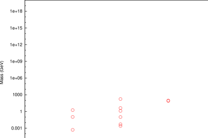
Forgetting for the moment the more concrete theoretical reasons (which we will review in the following chapter) to expect the observation of new phenomena at the energy scales of the LHC, we can make a plausibility argument for their existence by a simple observation. Figure 1.1 demonstrates the spectrum of known fundamental particles present in the SM that possess mass.333The neutrinos also possess mass, albeit a small one. However, only mass differences are known and we do not show them here. The vertical axis shows the mass in logarithmic scale, extending from to the scale , the fundamental scale of gravity, known as the Planck scale.444The Planck scale is the scale at which the strength of the gravitational interaction between particles becomes of order one. An estimate is given by , where is Newton’s gravitational constant. The Planck scale is the highest scale at which our current understanding of physics makes sense. By examining Fig. 1.1, one may observe something bizarre and slightly suspicious: many particles have been discovered with masses ranging from fractions of a GeV to fractions of a TeV, and one more (the Higgs boson) is predicted below the TeV scale, but no known particles exist above that scale! The question that arises is: why should there be such a ‘desert’ of energy (or mass) scales between the TeV scale and the Planck scale? If we do not accept the existence of such a puzzling absence of particles, then we can only conclude one of the following:
-
•
We do not currently possess the correct understanding of the fundamental scale of gravity, the Planck scale. Either there exists some specific mechanism explaining why such a large hierarchy arises between the TeV scale and the Planck scale, or the Planck scale is much lower than .
-
•
There exists a multitude of new particles and new interactions, waiting for potential discovery by future experiments.
Both of these prospects are very exciting. The LHC will be instrumental in exploring the TeV scale, perhaps revealing a whole new set of particles or phenomena that will provide an explanation for the above observation.
This thesis focuses on hadron colliders, of which the LHC is the most ‘powerful’ ever built. It is an extraordinary experiment, based on a collaboration which transcends borders, involving tens of thousands of researchers from more than a hundred nations. The task that particle physicists are facing at the LHC is non-trivial. Certain ingenuity is required if we wish to maximise the amount of physics results obtained from the experiments. A solid bridge of communication between the theorists and the experimentalists needs to be established. This is where phenomenology comes into play: it provides an interface between theory and experiment, for example through powerful computational tools, Monte Carlo programs, which we will be discussing in detail in chapter 3. These tools are indispensable to both experimentalists and theorists. In chapter 4, we make analytical phenomenological predictions of the effects of the theory of the strong force, quantum chromodynamics (QCD), to observables that experimenters will be using, either in their searches for new physics, or for better understanding of known SM processes. In the final chapter, 5, we take two well-motivated new physics scenarios and provide a phenomenological analysis to act as a guide for experimentalists in their search.
In another part of his 1900 talk in Paris, Hilbert asks the following:
‘Who of us would not be glad to lift the veil behind which the future lies hidden; to cast a glance at the next advances of our science and at the secrets of its development during future centuries?’
We hope that soon we will have reached such a point.
Chapter 2 The Standard Model and beyond
2.1 Introduction
In his popular science book ‘QED: The Strange Theory of Light and Matter’ [6], Richard Feynman writes:
Therefore the possibility exists that the three ’s and the photon are all different aspects of the same thing. Stephen Weinberg and Abdus Salam tried to combine quantum electrodynamics with what’s called the ‘weak interactions’ into one quantum theory, and they did it. But if you just look at the results they get you can see the glue, so to speak. It’s very clear that the photon and the three ’s are interconnected somehow, but at the present level of understanding, the connection is difficult to see clearly – you can still see the ‘seams’ in the theories; they have not yet been smoothed out so that the connection becomes more beautiful and, therefore, probably more correct.
Despite Feynman’s observation, the so-called ‘Standard Model’ of particle physics (abbreviated as SM) has been tremendously successful at describing experimental data. In fact, the SM can be arguably considered as the quantitatively most successful theory our species has ever constructed, with astounding agreement between theory and experiment: the anomalous magnetic moments of the electron and of the muon are amongst the most precise measurements in the whole of physics.
The ‘glue’-ing that Feynman refers to is the fact that the SM is a gauge theory of a product of gauge symmetry groups:
| (2.1) |
where the describes quantum chromodynamics (QCD) and the the electroweak (EW) theory. The symmetry, known as colour, is explicitly manifest in Nature, whereas the symmetry is broken down to via the Higgs Mechanism.
The Higgs Mechanism, introduced to explain the masses of fermions and bosons in the theory by breaking the electroweak symmetry, is currently the least understood part of the SM and is thus a source of inspiration to many extensions to the SM. Many of these extensions attempt to explain the so-called ‘hierarchy problem’, which can be briefly described as the lack of explanation for the stability of the Higgs boson mass against radiative corrections. Due to this issue and other open theoretical questions, the SM is often believed to be an incomplete description of particle physics. Its amazing success at describing experiments, however, ensures that it will be a subset of a ‘true’ theory, understood in the framework of effective field theories as capturing the low-energy limit of some more fundamental, microscopic physics [7].
In section 2.2 we give a general introduction to the SM at its current state, starting from the general principles for writing down a relativistic quantum field theory. We will be focusing on the phenomenological aspects of the EW theory and QCD and mathematical details will be kept to a minimum. In section 2.3 we examine some important open theoretical and experimental questions that suggest the need for extensions to the SM and present a brief overview of BSM theories.
2.2 The Standard Model
2.2.1 Gauge theories
Symmetries provide good candidates for underlying first principles in Physics. The gauge principle is an economical guide for using local symmetry to construct renormalisable quantum field theories. The fact that local invariance is required is motivated by the relativistic viewpoint: each observer, at every space-time point, possesses some freedom of convention. This of course may be considered by some as an aesthetical argument; however, the gauge principle has been proven to produce phenomenologically successful field theories and accounts for quantum electrodynamics (QED) as well as EW theory and QCD.
The gauge principle is most simply illustrated in the case of invariance under the unitary group , which yields an abelian gauge theory that describes QED. Consider the classical Lagrangian density111In what follows, and the rest of this thesis, we will be referring to the ‘Lagrangian density’ simply as the ‘Lagrangian’. describing the interaction of a spin 1/2, charged fermion field with the gauge field :
| (2.2) |
where is the field strength tensor and the covariant derivative is defined by , where and are respectively the mass and electric charge of and we have also defined the Feynman slash convention. The Lagrangian is invariant under the simultaneous gauge transformations:
| (2.3) | |||
| (2.4) |
where is an arbitrary function of space-time. Had we not included the field , the Lagrangian would not have remained invariant under the local transformation of the field alone, owing to the derivatives present in the fermion kinetic terms. This can be seen explicitly if we examine the transformation of the term under Eq. (2.4):
| (2.5) |
which is evidently not invariant unless we use the covariant derivative, which introduces , to cancel out the extra term:
| (2.6) | |||||
Thus, the requirement that the Lagrangian (and hence the equations of motion) is invariant under local transformations requires the existence of a gauge field . This field corresponds to the electromagnetic field and hence to the photon.
2.2.2 Electroweak theory
As we alluded in the introduction, the electroweak sector of the SM can be described by a non-abelian gauge theory based on the group , where the subscript indicates the left-handed chiral nature of the coupling of the gauge fields and is the hypercharge, to be distinguished from the electromagnetic charge, . The quantum number is referred to as the weak isospin. We can separate the Lagrangian into three parts as
| (2.7) |
where , and correspond to the gauge bosons, the Higgs field and the fermions respectively.
2.2.2.1 Boson masses
The gauge boson Lagrangian now contains two gauge fields:
| (2.8) |
where the and are the field tensors corresponding to the and symmetries and the index labels the weak isospin quantum numbers:
| (2.9) |
where the are the group structure constants (the alternating tensor in the case) and is the charge. It is important to note that the non-abelian field tensor now contains a self-interaction term , a feature that is even more significant in non-abelian gauge theory, as we shall see.
The symmetry is not manifested in nature. It is in fact, a spontaneously broken symmetry: the and gauge bosons are massive. The minimal way to break it within the SM and give masses to the gauge bosons, while preserving the gauge-invariant nature of the theory, is to introduce the complex scalar Higgs field that is an doublet and possesses hypercharge :222The hypercharge for the Higgs field could have been chosen . The choice affects the hypercharges for the rest of the matter content in the theory. The relation between electric charge, hypercharge and the third component of weak isospin will contain factors of 2 accordingly.
| (2.12) | |||||
| (2.14) |
where the meaning of the labels on the components will become apparent subsequently. The corresponding Lagrangian, is given by
| (2.16) |
where the covariant derivative, which introduces the interaction between the Higgs field and the gauge fields, is defined by
| (2.17) |
In the above, we have suppressed weak isospin indices, the are matrix representations of the generators and and are the and gauge charges respectively. The potential term is given a special form containing quadratic and quartic terms, commonly referred to as the ‘mexican hat’ potential:
| (2.18) |
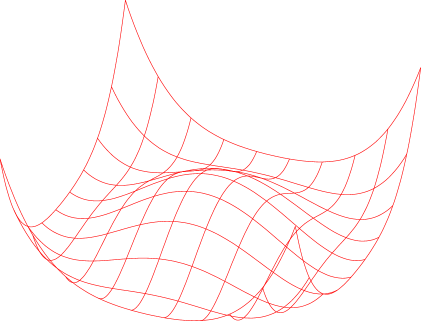
and the constants are chosen such that . This potential possesses a minimum at , an unstable maximum at the origin and goes off to positive infinity as (hence the resemblance to the mexican hat). Figure 2.1 illustrates the shape of the potential on the complex plane.
To break the symmetry, a particular direction (referred to as a ‘vacuum expectation value’ or VEV) in the space for the minimum of is chosen:
| (2.21) |
Notice that, at the minimum, the theory still possesses a residual symmetry. To determine the properties of the theory at this minimum, we need to expand the fields about it, using an transformation of the field:
| (2.22) | |||||
| (2.25) |
where we have three components and one scalar degree of freedom, . At first order this is just an expansion of the field about the minimum. Since the Lagrangian of Eq. (2.16) is gauge-invariant, we should simultaneously perform an gauge transformation:
| (2.26) |
We obtain the following form for the Higgs boson Lagrangian:
| (2.27) |
where we have used the vector , a unit vector along the direction of the Higgs boson VEV. Evidently the three degrees of freedom from the field do not appear explicitly in the Lagrangian. These degrees of freedom have been absorbed by the gauge bosons and provide the longitudinal degree of freedom: a massive vector boson has three polarisation states whereas a massless one has two.
We now consider the terms quadratic in the vector boson fields:
| (2.28) |
We need to rewrite this in ‘diagonal form’, i.e. in terms of mass eigenstates. We define two electrically neutral fields and :
| (2.29) |
where we have also defined the electroweak mixing angle, .333The current Particle Data Group value is [13]. Using the definitions of Eq. (2.29) we have
| (2.30) |
from which we can now deduce the vector boson masses:
| (2.31) |
Thus, with the particular choice for the Higgs boson representation, masses have been generated for the weak vector bosons, and , while one field, , has remained massless. This corresponds to a -symmetric force which we identify with QED and a boson which we identify with the photon, . We can thus write the following symmetry breaking relation:
| (2.32) |
and we can associate the different charges of fields by
| (2.33) |
where is the electromagnetic charge, is the third component of weak isospin and is the hypercharge. is essentially the only remaining unbroken generator. We can now see that the upper component of the Higgs doublet has , whereas the lower one has charge , which explains why the VEV was chosen as in Eq. (2.21).
2.2.2.2 Fermion masses and couplings
Introducing fermion masses explicitly into the fermion Lagrangian would break gauge invariance. The Higgs mechanism in its simplest form is the conventional method to give masses to the SM fermions without any adverse effects. The choices of fermion representations in the SM and their charges are given in Table 2.1, for the first generation. The SM has been observed to contain three ‘copies’ of this structure: three generations.
| Representation | |||
|---|---|---|---|
| 0 | -1 | -1 | |
| 0 | |||
| - 1/2 | |||
| -1 | |||
| 0 | 0 | 0 | |
| 0 | |||
| 0 | +2/3 |
Notice that the difference between the hyperchages of the singlet (right-handed) and doublet (left-handed) is , which allows us to use the Higgs doublet (with ) to form gauge-invariant terms:
| (2.38) | |||||
| (2.43) | |||||
| (2.44) |
Thus, when the Higgs field obtains a VEV and the symmetry is broken, we obtain terms quadratic in the fermion fields: mass terms proportional to the VEV, , and mixing terms between the fermions. To take care of this mixing we conventionally define
| (2.51) |
where is known as the Cabbibo-Kobayashi-Maskawa (CKM) matrix.444Kobayashi and Maskawa were awarded the Nobel Prize in 2008, on work related to the CKM matrix, and specifically ‘for the discovery of the origin of the broken symmetry which predicts the existence of at least three families of quarks in nature’ [14]. is a unitary matrix, given by
| (2.55) |
and can be parametrized by three mixing angles and a charge-parity (CP) violating phase. In the SM, this phase provides a source of CP violation, observed experimentally via mixing in the neutral kaon system (- mixing) [11]. See appendix C for parametrizations of the CKM matrix and measured values of its matrix elements.
In practical calculations, the CKM matrix elements can be inserted into the amplitude of diagrams where a boson couples to quarks and . If we define the right- and left-handed projection operator for fermions, , we may write down the interaction term between the SM fermions and and the boson:
| (2.56) |
where for leptons () and for quarks and .
2.2.3 Quantum chromodynamics
Quantum chromodynamics (QCD) is also formulated in terms of a gauge theory, based on the non-abelian group . It possesses several distinct features: it is unbroken in Nature, contains self-interacting degrees of freedom, the gluons, and exhibits asymptotic freedom, which reveals that only in the short-distance limit we can use perturbative methods legitimately.
We will briefly review the construction of the theory and subsequently present perturbative tools that will be employed in calculations that will follow in this thesis.
2.2.3.1 SU(3) gauge theory
The fermions that carry charge, or colour charge, are the quarks. The full quantum Lagrangian is given by
| (2.57) |
The expression for the classical Lagrangian is similar to what we have written down for the QED and EW theories:
| (2.58) |
where the sum over the index is over the eight colour degrees of freedom of the gluon field , the sum over flavours is over the quark flavours and the field strength tensor is defined as
| (2.59) |
where is the strong charge and the are the structure constants of . We may also define the strong coupling constant . The covariant derivative is defined according to whether it acts on triplet or octet fields:
| (2.60) |
where and are generators (matrices) in the fundamental and adjoint representations of respectively. They satisfy the following relations:
| (2.61) |
The following identities are true for gauge theories:
| (2.62) |
which imply that for QCD, for which : , and . In practical calculations an explicit representation for the is not necessary, and the identities of Eq. (2.62) are used.
The classical Lagrangian, Eq. (2.58), is invariant under the simultaneous transformations:
| (2.63) |
where are eight arbitrary real functions of space-time.
The Lagrangian of Eq. (2.58) cannot be used immediately to calculate Feynman rules for QCD: in this form, a propagator for the gluon field cannot be defined.555The same issue arises when defining the photon propagator in QED. We can exploit gauge invariance to add a gauge-fixing term to the QCD Lagrangian which amends this issue:
| (2.64) |
where is an arbitrary parameter. Provided we work in the covariant gauge, that is, a gauge in which we choose , we have not made any changes in the physics and we can now define a propagator for the gluon fields.
Finally, it is necessary to add an extra term to the Lagrangian which is related to the need for ghost particles, , whose purpose is to cancel unphysical degrees of freedom that may arise when renormalising a non-abelian gauge theory. For further details on non-abelian gauge theory renormalisation and the need for ghost fields, see [8].
2.2.3.2 Renormalisation and the running of
Besides the masses of the quarks, the only other parameter which appears in the QCD Lagrangian is the strong charge,666In practical calculations one usually employs rather than . . One should be cautious however: parameters in a Lagrangian are not necessarily physical quantities. Physical observables can be calculated as functions of these parameters, in this case of . What we would like to do is reformulate the theory so we can write a physical observable as a function of another. This process is called renormalisation.
As an illustrative example, as given in Ref. [9], consider the quark-gluon vertex shown in Fig. 2.2.
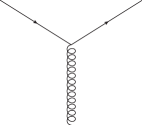
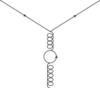
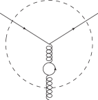
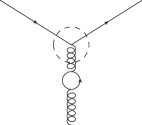
Figure 2.2a shows the lowest order of the vertex in perturbation theory, for which we can define to be the strength. If we now start considering higher orders, and specifically part of the one-loop correction shown in Fig. 2.2b, we must decide whether we will include this as part of the vertex, as in Fig. 2.2c, or as part of the rest of the diagram, as in Fig. 2.2d. To do this we choose some scale , called the renormalisation scale, above which the loop is part of the vertex, as in Fig. 2.2c, and below which it is part of the rest of the diagram, as in Fig. 2.2d. This scale should not have any physical significance: it is simply a device we introduce to avoid double-counting. Due to this, should not affect any physical prediction. However, the strength now becomes a function of the scale .
We can see the effect of this procedure on the theory by considering a dimensionless physical observable that is a function of a physical scale . After applying the above renormalisation procedure, the observable can only be a function of , and . Dimensional analysis restricts to depend on and only through their ratio, giving
| (2.65) |
We can now employ the fact that a physical observable cannot depend on the value of the renormalisation scale, and write, using the chain rule:
| (2.66) |
where we have defined
| (2.67) |
An important observation is that the -dependence of the quantity would not have come about in a classical theory: it is a feature of the renormalised theory which arises due to the introduction of the scale .
Even though the -function of QCD is currently known to four-loop accuracy,
| (2.68) |
only the one-loop result is necessary for qualitative understanding of QCD:
| (2.69) |
For most phenomenology the number of active quark flavours can be taken to be and hence the -function is negative when is small. This implies that the running coupling decreases to zero as an inverse power of . To one-loop order, we have
| (2.70) |
Hence QCD interactions become weak at high energy, a feature called asymptotic freedom, and strong at low energy. This is in contrast to QED, where the observed charge of the electron is smaller at large distances. This can be thought of as being due to the self-interactions of the gluons: emission of virtual gluons, which are themselves charged, causes the colour charge of the source that emitted them to ‘leak out’ to the vacuum. In effect, this reduces the colour force at short distances since the interaction between distributed charges that overlap is weaker than that between point charges.
2.2.3.3 Parton evolution
Free quarks or gluons have not been observed in Nature. This has led to the confinement hypothesis: the only energy eigenstates of QCD that can exist in Nature have to be colour-neutral (or colour-singlets). There is strong circumstantial evidence in favour of the hadrons as bound states of quarks and anti-quarks. For example, there exists quantitative understanding of high energy inelastic scattering of hadrons once they are taken to be composites of quarks and gluons. In fact, hadron-hadron and hadron-lepton scattering can be described in terms of perturbation theory and the parton model, a direct consequence of the property of asymptotic freedom. The basic assumption of the parton model is that interactions of hadrons are due to interactions of more elementary entities, called partons, which turn out to be the quarks and gluons of QCD. The number and momenta of partons are most conveniently described in terms of parton density functions (PDFs). Theoretical and experimental details on the parton model can be found in [10].
The PDFs are fundamentally non-perturbative and at present cannot be predicted from first principles. However, the evolution equations for their scale-dependence can be derived (see, for example, [10]). We denote the fraction of momentum of the proton that a parton possesses at scale as . The momentum fraction distribution is then denoted by . The equation describing the evolution of , known as the DGLAP (Dokshitzer-Gribov-Lipatov-Altarelli-Parisi) equation, takes the following form:
| (2.71) |
where are the so called (regularised) splitting functions, related to the probability of finding a parton in a parton and the integral is taken over all possible momentum fractions for the splittings, . The regularised splitting functions at leading order are given by
| (2.72) | |||||
where we have used the so-called ‘plus’ prescription,
| (2.73) |
and the values of the constants , and for QCD have been given in section 2.2.3.1.
2.2.3.4 Parton branching
Perturbative calculations in QCD are hard beyond leading order: the work involved increases roughly factorially with the order. However, there are cases when we cannot truncate the series to a fixed order since there are higher order terms that are enhanced in certain regions of phase space. Such a region is collinear parton emission from a parton involved in a scattering process. This can be either an incoming parton or an outgoing parton. Branchings of outgoing partons are called ‘time-like’ (Fig. 2.3) and branchings of incoming partons are called ‘space-like’ (Fig. 2.4).
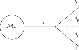
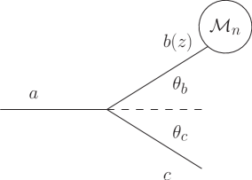
We consider the kinematics for the time-like branching shown in Fig. 2.3 first. Our aim is to calculate the modification to the -body cross section when we have a single branching in the collinear approximation. We define the opening angle between the outgoing partons and as . The collinear approximation implies that . If we neglect the parton masses then and . If we then define , using , we may write
| (2.74) |
where and are the corresponding energies of the partons and . Defining the energy fraction of the splitting, , by
| (2.75) |
can then be approximated for small as
| (2.76) |
Due to the propagator factor, the -body matrix element squared, , is proportional to . In fact, it can be shown that it can be written in terms of the -body matrix element squared as
| (2.77) |
The splitting function in this case, , is ‘unregularised’, i.e. it may diverge as or . It will be shown later how to obtain a regularised splitting function when including the virtual corrections to the differential cross section, for the case of space-like branching (section 4.2). The origin of the collinear enhancement is now obvious: it is due to the factor which diverges as , i.e. when the internal parton line is on-shell.
We can use Eq. (2.77) to compute the cross section for one branching in terms of that for no branchings, using the following relations:
| (2.78) |
where is the flux factor for the initial state and is the relevant -body phase space. It can be shown that
| (2.79) |
where is the azimuthal angle related to the branching. Hence, in the collinear approximation, when all angles are small, we have derived the relation between the -body differential cross section and the differential cross section for one time-like emission,
| (2.80) |
where an average/sum over initial/final spins has been taken. We can repeat the same procedure for space-like branchings (Fig. 2.4) for which we define . We then have and the phase space factor becomes
| (2.81) |
where . But in this case the initial-state flux factor, , changes by a factor of because of the change of energy of the incoming parton from to . Thus, it turns out that the expression for space-like branching is identical to the one for time-like branching, Eq. (2.80).
2.3 Beyond the Standard Model
2.3.1 The need for BSM physics
The standard model is phenomenally successful at describing strong, weak and electromagnetic interactions, with precision results up to . Given its success, why don’t we just look for the ‘missing’ Higgs particle and declare the end of particle physics once we discover it? The reason is that there are conceptual and phenomenological hints that the SM is incomplete. The conceptual issues include the multitude of unexplained parameters, family replication and flavour hierarchies, the inability of the SM to incorporate gravity and the hierarchy problem. Phenomenological hints are neutrino masses, Dark Matter, the cosmological vacuum energy (also known as Dark Energy) and the quest for Grand Unification and coupling constant merging. We discuss a few of these issues here.
2.3.1.1 The hierarchy problem and new physics
An important conceptual issue, known as the hierarchy problem, concerns the Higgs field. Essentially the problem arises since, in its usual Standard Model incarnation, the Higgs boson is considered to be a fundamental scalar. Fundamental scalars suffer from radiative instability in their masses due to radiative corrections. The three most ‘dangerous’ contributions from radiative corrections to the Higgs boson mass in the SM come from one-loop diagrams with top quarks, gauge bosons and the Higgs boson itself, as shown in Fig 2.5.

The contributions to the Higgs boson mass squared are proportional to a cut-off scale squared, , with the top contribution being negative and the gauge and Higgs boson contributions being positive. If is set to be the Planck scale, , then the Higgs boson mass ought naturally to be of that order, barring any unnatural cancellations between the positive and negative contributions. On the other hand, experimental evidence shows that the Higgs boson should be light: its mass should be , assuming no new physics [13]. To achieve this, the cut-off scale should be much lower than the Planck scale and new physics, possibly in the form of new resonances, is expected to appear at the electroweak scale .
2.3.1.2 The little hierarchy problem
If new particles are indeed responsible for cancelling the quadratic divergences to the square of the Higgs boson mass, their masses should be by naturalness. However, current experimental data already set some constraints on possible new physics at the TeV scale. For example, absence of nucleon decays and strong bounds on flavour-changing neutral currents indicate that these effects cannot receive any significant contributions from TeV-scale physics. Precision electroweak measurements put constraints on operators arising by exchanging new heavy particles and scales which suppress them are required to be larger than [15]. Therefore, there exists an issue of compatibility between the experimental data and the expectation of the masses of the new particles required in order to satisfy the naturalness of the low Higgs boson mass. This is sometimes referred to as the ‘little hierarchy problem’.
A possible ‘solution’ to this problem relies on the fact that the quadratic sensitivity to the high energy physics of the Higgs boson mass is a result of loop contributions: to cancel the quadratic divergences, the new TeV-scale particles only need to appear in interaction vertices in pairs or more. Therefore, we can suppress the tree-level contributions, while maintaining the cancellation of the loop contributions, by introducing a new symmetry acting on the new particles, under which all the SM fields are neutral. The simplest, and most common, choice is a symmetry, or parity.
2.3.1.3 Dark Matter
The nature of Dark Matter (DM) has been an open question in astrophysics since the initial observations by Fritz Zwicky in 1933 which required the existence of non-luminous, weakly interacting matter to explain the orbital velocities of galaxies in clusters. Following the initial discovery, observations have indicated that galaxy rotation curves do not fall off with radial distance from the galactic centre and evidence from the cosmic microwave background (CMB) indicates that DM makes up about 25% of the energy density of the Universe [16].
There are two basic types of candidates for DM. The first is Massive Compact Halo Objects (MACHOs). MACHOs are objects of baryonic origin such as black holes, brown dwarf stars and giant planets. It has been shown, however that MACHOS cannot account for more than 20% of DM [17]. The second type of candidates are weakly interacting particles. The only candidates within the SM, the neutrinos, do not possess the necessary density to compose the Dark Matter. In addition, the existence of hot (i.e. relativistic) DM is not consistent with observations and hence any candidates should be relatively heavy. Thus DM is thought to consist of cold (i.e. non-relativistic), stable, or at least meta-stable [18, 19], massive particles which appear in theories beyond the SM. These are usually called Weakly Interacting Massive Particles, or WIMPs. There are good arguments that these particles might appear at the TeV scale [20].
2.3.1.4 Dark Energy
Strong evidence for the existence of Dark Energy comes from distant supernovae observations, indicating that our Universe is currently undergoing an accelerated expansion. The question of the nature of Dark Energy is considered by theorists to be even more severe than the Dark Matter problem, not only because Dark Energy is thought to contribute about 70% of the energy density of the Universe, but also because we currently have no strong theoretical explanations for it: it is totally mysterious. It could possibly be the vacuum energy, in the form of a cosmological constant. The issue is much worse than the previously mentioned hierarchy problem: calculations of the energy density of vacuum in quantum field theory, with a cut-off at ,777This scale could be the Grand Unification scale, for example. give a result for a cosmological constant of the order of , whereas the measured value of the dark-energy density is [21]. It is likely that solving the problem requires a complete quantum theory of gravity [22].
2.3.1.5 GUTs and coupling constant merging
A troubling feature of the Standard Model is the fact that it contains almost 20 parameters. It is thought that a fundamental theory of nature should be able to explain the origin of their values through some underlying principle. We would also need to address the issue Feynman wasn’t comfortable with at the conception of the Standard Model: the fact that the different components ‘have not yet been smoothed out’. It basically boils down to the fact that we have three gauge couplings of different magnitudes. In mathematical terms, the question is why is the gauge group of the Standard-Model semi-simple and not simple?
A resolution to this issue is to assume that the underlying gauge symmetry of nature is in fact a simple group, but it is broken at some high energy scale down to the gauge group of the SM. For example, the underlying gauge group could be the group, which can be shown to contain an subgroup. The group can then be easily broken down to the SM group via the introduction of a set of Higgs fields [21]. Although can successfully incorporate the SM, it predicts proton decay with a lifetime that has already been excluded [23]. Nevertheless, it is a simple example of a Grand Unified Theory (GUT).
A GUT can possibly solve the problem of seemingly separate gauge couplings. As we have already demonstrated in the case of the strong coupling constant, , the gauge couplings are scale-dependent quantities. If the hypothesis of unification is to hold, they must all equal each other at some scale, the grand unification scale. Below this scale, the simple group (e.g. ) is broken down to the SM group and the separate couplings have different behaviour. In fact, below the grand unification scale, the couplings for each group , and evolve according to the respective -functions with no memory of the simple group they originated from. If the exercise is performed, evolving from low to high scale, however, it is found that the unification of the couplings in the Standard Model is a ‘near-miss’, as can be seen by the dashed lines in Fig. 2.6.

2.3.2 Survey of BSM theories
2.3.2.1 Supersymmetry
Supersymmetry is one of the most popular extensions to the Standard Model, and not without good reasons. Conceptually it is very appealing: it is the only possible extension to the spatial symmetries of the theory in flat, four-dimensional space. It appears to be able to accommodate a solution to the hierarchy problem, contains natural candidates for Dark Matter and solves the ‘near-miss’ of the gauge-coupling unification in the SM. It is also a powerful tool for understanding quantum field theories, especially in the non-perturbative regime [25].
Supersymmetry introduces fermionic operators and to the Poincaré generators (corresponding to translations) and (corresponding to rotations and Lorentz boosts).888Hence, the Poincaré group corresponds to the basic symmetries of special relativity. The new operators satisfy the following anti-commutation relation:
| (2.82) |
where is the 4-vector of Pauli matrices. The anti-commutation relation implies that two symmetry transformations have the effect of a translation. This is to be expected since the operators themselves carry spin angular momentum, so it is clear that supersymmetry must be a space-time symmetry.
Let be a bosonic state and a fermionic state. Then we have, schematically,
| (2.83) |
and, as a result,
| (2.84) |
Supersymmetry is a symmetry between bosonic particles and fermionic particles. The matter fields (in the fundamental representations) of the Standard Model, fit into chiral multiplets, while the gauge fields fit into vector multiplets. In supersymmetry, a chiral multiplet contains a fermion field and a scalar field, related by a supersymmetry transformation such as the one described by Eqs. (2.83) and a vector multiplet contains a vector field and a fermion field also related by the same transformation. If supersymmetry is exact (i.e. unbroken) the particles related to fields in the same multiplet should possess the same mass.
The minimal additional content of a supersymmetric theory to the matter fields of the SM consists of a (super-)scalar for each chirality of the SM fermions and a (super-)fermion for each SM vector boson. The Higgs boson sector for electroweak symmetry breaking becomes more complicated, requiring the introduction of a second Higgs doublet, otherwise the electroweak gauge symmetry would suffer a gauge anomaly. The conditions for cancellation of gauge anomalies are already miraculously satisfied in the SM by the known quarks and leptons, but in a supersymmetric theory, the multiplet which contains the SM Higgs boson will now contain a fermionic partner. This would spoil the anomaly cancellation, but can be avoided if a second doublet which has is introduced, so that the contributions from the two fermionic members of the Higgs multiplets are cancelled out. Furthermore, the doublet is required so that masses can be given to the down-type quarks and charged leptons [24].

The Minimal Supersymmetric Standard Model (MSSM) provides an elegant solution to the hierarchy problem of the SM: the supersymmetric partner corrections cancel out the quadratically divergent SM particle corrections to the square of the Higgs boson mass, as illustrated in Fig. 2.7. Supersymmetry can also accommodate candidates for Dark Matter. As we have mentioned in section 2.3.1.2, to solve the little hierarchy problem we need to introduce a new discrete symmetry, or parity. In the MSSM, and in other supersymmetric models, -Parity is introduced, under which the super-partners are odd and the SM particles are even. If -parity is exact, the lightest supersymmetric particle (LSP) cannot decay to lighter SM particles and thus may be stable and contribute to Dark Matter.
Exact supersymmetry is of course not manifested in nature, otherwise we would have already observed the super-multiplets. A method to break supersymmetry is thus required; in fact this is where the elegance of the theory ends and the complications begin: as a result of the breaking, many free parameters are added to the model. To maintain the successful cure for the hierarchy problem, resulting in the observed and masses, the masses of super-partners should be around the TeV scale, with the lightest ones at most about [24].
2.3.2.2 Extra Dimensions
Another possibility of extending the space-time symmetries of Nature is to introduce extra spatial dimensions. This has been a long-discussed idea and has re-surfaced in different contexts. There are many flavours of models with extra dimensions, each attempting to address different issues that plague the SM: e.g. Universal Extra Dimensions [26] or Randall-Sundrum type scenarios [27].
The Randall-Sundrum scenario is particularly interesting. In its simplest form, it is a 5-dimensional theory. The extra dimension is an interval, with the surfaces (or ‘branes’) at the end of each interval being (3+1)-dimensional. One surface is at and the other at , where is a length related to the extra dimensions. The metric changes from to as where is a constant. This implies that all the length and energy scales change with . If the fundamental scale is the Planck scale, , the brane carries physics at , but all energy scales are ‘red-shifted’ by the exponential factor until the other brane is reached, where we would have an exponentially smaller scale. In particular, this scale can be the electroweak scale: . In fact this method ‘shifts’ the hierarchy problem to a problem of finding the proper mechanism to fix the size of the extra dimensions. The Randall-Sundrum scenario can also potentially incorporate a mechanism that explains the flavour structure and mass hierarchy of the SM [28].
Very often, extra-dimensional models suffer from a ‘little hierarchy’ problem and a discrete parity needs to be introduced to restrict the production of heavier resonances to pairs. This is sometimes called ‘Kaluza-Klein’ parity (KK parity). The lightest KK resonance is sometimes also considered to be a viable Dark Matter candidate.
2.3.2.3 Strong dynamics
Strong coupling dynamics can provide an elegant and natural solution to the hierarchy problem. It is natural in a literal sense since we have already observed an example in Nature in which a large hierarchy arises: between the Planck scale and the proton mass scales (). This is a result of the running of the QCD coupling constant and the strong coupling regime in the infrared.
In technicolour models, as some strong dynamics models are usually called, mass is given to the electroweak gauge bosons via some new strong dynamics. Extensions to these models allow mass to be given to the SM fermions as well. In typical types of extensions we obtain large flavour-changing neutral currents which are highly constrained by experiment. Technicolour models also have trouble facing the electroweak precision tests. Minimal Walking Technicolour (MWTC) [29] is a model which has the smallest deviation from precision data, with the most economical particle content. In MWTC theories the coupling remains large and nearly constant over a wide range of energy scales. Technicolour theories have also been combined with supersymmetry to alleviate some of the issues present [30].
Strong dynamics theories may contain composite fermionic or bosonic resonances or composite Higgs particles. We will examine a model which contains scalar leptoquark resonances in section 5.3.
2.3.2.4 Dimensional deconstruction and Little Higgs models
Dimensional deconstruction involves building extra dimensions instead of starting with them [31]. The idea can be used to construct renormalisable four-dimensional gauge theories that dynamically generate extra dimensions. In this framework, extra dimensions can be used purely as an inspiration and may be discarded in the end, together with all the issues they introduce (for example, without the need of justification of the size of the extra dimension). As a result, realistic theories of electroweak symmetry breaking in four-dimensions can be constructed, with the new feature that they are perturbative (as supersymmetry is) and insensitive to high energy details up to a cut-off scale much larger than .
‘Little Higgs’ models are such models, inspired by the method of dimensional deconstruction [32], although most do not have a simple five-dimensional or ‘theory space’ interpretation. In Little Higgs models a special ‘collective’ pattern is created in which the gauge and Yukawa couplings break some global symmetries. As a consequence of this special pattern, the one-loop contribution to the Higgs boson mass is not generated. This can be viewed as the cancellation between divergences caused by the SM particles (Fig. 2.5) and new resonances, as in supersymmetry. Unlike supersymmetry, the new resonances have the same statistics as their SM counterparts. The remaining corrections to the Higgs boson mass parameter are smaller and no fine tuning is required to keep the Higgs boson light. At energies of , the Little Higgs description becomes strongly-coupled and the model needs to be completed in the ultraviolet regime, for example by a QCD-like gauge theory with a confinement scale around [33]. Note that in phenomenologically viable Little Higgs models, a discrete parity, called -parity, needs to be introduced to solve strains that arise from the electroweak precision tests [34, 35]. The phenomenological consequences are similar to those in supersymmetry: new heavy resonances will be pair-produced and the theory may contain Dark Matter candidates.
2.3.2.5 String theory and all that
String theory [21] was ‘discovered’ by accident in the late 1960s, first proposed as a theory of strong interactions. It was later dismissed as a valid theory of hadronic physics, but some theorists considered the fact that it contained spin-2 resonances as an indication that it could possibly lead to a theory of gravity. A lot of work has been done in the ‘framework’ of string theory and it has since become a popular candidate for a quantum theory of gravity. However, organising principles for the ‘theory’ do not exist and at present it seems that the number of possible solutions is practically infinite.
Another candidate for a theory of quantum gravity is ‘loop quantum gravity’. It is a non-perturbative approach to a quantum theory of gravity, in which no classical background metric is used. One of the consequences is that quantities such as area and volume are quantised in units of the Planck length. It has modest aims, not attempting unification; rather, its goal is to quantise Einstein’s general theory of relativity in four dimensions [36].
Whatever the theory of quantum gravity looks like, what is certain at this point is that we need a major revision of our understanding of the nature of space-time to discover a path towards it.
Chapter 3 Monte Carlo methods and event generators
3.1 Introduction
Theories of physical systems are formulated in terms of ‘equations of motion’. These are usually differential equations which describe the rate of change of variables with respect to system parameters, such as time. For concreteness, let us assume that the rate of change of a particle’s position in one dimension, , is given by the following differential equation:
| (3.1) |
where is a given function of time. To calculate the displacement of the system from to , we need to integrate the differential equation:
| (3.2) |
In fact, a vast majority of problems in Physics can be reduced to solving particular integrals. Most of these integrals cannot be solved analytically, forcing us to resort to numerical techniques to evaluate them.
In one dimension, calculating integrals numerically is just a matter of applying certain well-known techniques, such as the trapezium rule, Simpson’s rule, gaussian quadrature and so on. These take the values of on points , at certain fixed intervals, and yield an estimate of the integral. These ‘quadrature’ methods are based on approximating the function with some polynomial. An alternative technique is based on the fact that the value of the integral can be recast as the average of the integrand:
| (3.3) |
We can approximate the average of the integrand by taking values of , uniformly distributed on , and hence obtain a reasonable estimate of :
| (3.4) |
The order in the sum in Eq. (3.4) is not of any significance so it is possible to draw the values of randomly. We can then write
| (3.5) |
where is a random number111A random number is one whose value is unpredictable from any initial information. In practice pseudo-random numbers are used in Monte Carlo event generators. These are sequences of numbers which are fully deterministic, but are supposed to be indistinguishable from random numbers. We will assume that a pseudo-random number generator has been provided and we will not make the distinction in this thesis. on the interval . This method of using random numbers to aid the calculation of integrals is known as ‘Monte Carlo’ integration.222The name is, of course, inspired by the ‘Casino de Monte Carlo’ which is a ‘legendary casino, a jewel of the arts ‘Belle Epoque’, the absolute reference for all players. Its wide range of table games is the most prestigious and the most complete in Europe’ [37]. The only association of the author of the thesis to the famous casino appears at http://www.hep.phy.cam.ac.uk/theory/andreas/mc.jpg. If we assume , we can estimate the accuracy of the method using the Central Limit Theorem. The distribution of will tend to a Gaussian with standard deviation , where is the standard deviation of the values of . This implies that the inaccuracy of our estimate simply decreases as .
In particle physics the dimensionality of the integrals is usually very large and variable: for an -particle final state, there are dimensions, coming from the three components of momentum and taking into account the total 4-momentum conservation, plus flavour and spin labels. Table 3.1 shows the rate of convergence of the various integral approximation techniques in -dimensions: the ‘quadrature’ rules all suffer from the problem that they converge in accordance to , the number of points along each axis.333However this is only true for the quadrature methods if the derivatives exist and are bounded. The convergence of the Monte Carlo technique overtakes each of the methods mentioned at and respectively and hence it is well-suited for the high-dimensional integrals that appear in particle physics.
| Technique | Convergence |
|---|---|
| trapezium | |
| Simpson’s | |
| th-order gaussian quadrature | |
| Monte Carlo |
The Monte Carlo integration method in fact possesses many advantages over numerical quadrature methods: it converges fast in many dimensions, it can handle complex integration regions, it has a small ‘feasibility limit’ (the number of function evaluations which must be made for the method to work) and it is easy to estimate the accuracy of the result. Moreover, it is useful in the study of fundamentally random processes since there can be a direct correspondence between the parameter space points and actual events being modelled. This is one of the main reasons why the Monte Carlo method has become an important tool for collider experiments, through its use in constructing event generators and detector simulators.
3.2 Monte Carlo event generators
An event generator can be defined as any program which aims to simulate individual events, rather than the bulk properties of a physical process. Using the Monte Carlo method, an event generator is capable of simulating a wide range of interesting processes that are expected at hadron colliders such as the LHC.
As we have already noted at the end of the previous section, in particle physics the Monte Carlo method is closely related to the physical process under study in a way that allows us to make a direct connection between phase space points and events. The Monte Carlo method can be used to generate ‘unweighted’ events which can be manipulated like those obtained by experiment.
3.2.1 Unweighted event generation
The unweighting of events (or phase space points) is performed by a method called ‘hit-or-miss’. The method can be briefly described in the following steps:
-
•
We find the maximum of the distribution in the interval , , during an initial sampling. This is taken to be the maximum weight in the integration region.
-
•
In a subsequent sampling process, we choose whether we keep (accept) or throw away (reject) a randomly chosen event with properties given by , with probability . We thus end up with a sample of events which have been ‘accepted’.
-
•
During the initial sampling, the value of the integral, , can also be calculated using Monte Carlo integration as described by Eq. (3.5).
It should be understood that is now a multidimensional phase space point. The above steps can be translated to particle physics ‘language’ readily: the point would be a set of particle momenta and other quantum numbers, would be the matrix element squared for the configuration and would be the total cross section within the cuts set by and .
Both the convergence of the integral and the event generation efficiency can be improved if importance sampling is employed. The basic idea is to perform a Jacobian transformation so that the integrand is flatter in the new integration variable, thus reducing the standard deviation of the weights. Using importance sampling can improve the efficiency by many orders of magnitude.
3.2.2 General features of event generators
We outline the components of an event generator. For further details the recent review [38] is useful. We also discuss jets: although not explicitly part of the event generation, they are important for making the connection between the parton picture, arising from the theoretical calculations, and the hadrons observed in experiments.
3.2.2.1 Hard subprocesses
A particle physics event generator has at its core the simulation of ‘hard subprocesses’: particle scattering at large invariant momentum transfer. These processes are calculable in the framework of QCD, as it becomes asymptotically free at high energy and hence perturbative.
Unweighted hard scattering events are produced using the ‘hit-or-miss’ method as described in section 3.2.1. In the case of hadron colliders, with incoming hadrons and , partons and are ‘extracted’ from each respectively, with corresponding momentum fractions and . The probability density functions for the momentum fractions are then given by the relevant Parton Density Functions (PDFs): and , as defined in section 2.2.3.3. The cross section for the hard subprocess , can then be calculated by assuming that the non-perturbative hadron physics and the short-distance hard physics can be factorized [38]:
| (3.6) |
where and are the relevant factorisation [10] and renormalisation scales and the parton-level differential cross section may be written as
| (3.7) |
where is the final-state phase space, is the partonic centre-of-mass energy squared in terms of the hadronic centre-of-mass energy squared, , and is the matrix element squared for the process, averaged over initial spin and colour. The phase space over the final-state particles is given by
| (3.8) |
where and are the initial-state momenta.
3.2.2.2 Parton showers
The particles which participate in the hard subprocesses at hadron colliders are likely to carry QCD charge. Of course, this is always true for the incoming partons. Inevitably, colour-charged particles will radiate via the QCD interaction: quarks and gluons can radiate gluons, gluons can branch out to quark-anti-quark pairs. This is in accordance with the parton branching picture we presented in section 2.2.3.4, where we wrote down the expression for the differential cross section for a single branching, Eq. (2.80). This equation contains a factor, and hence the phase space region is enhanced. This is in fact a collinear-enhanced region, since, as we have already shown (Eq. 2.76), , where is the opening angle for the branching.
The Monte Carlo method is well-suited for describing parton branching. This is done in terms of the Sudakov form factor, which forms the basis of the ‘parton shower’. The Sudakov form factor,
| (3.9) |
is simply the probability of a parton evolving from scale (squared) to without branching, for a certain type of evolution (a parton evolving to a parton ). The integral over would diverge at and and so needs to be cut-off at appropriate values, functions of the cut-off scale . The Monte Carlo branching algorithm, details of which can be found in [10], evolves the parton from squared scale and momentum fraction to in steps in space. The algorithm takes into account collinear enhancements to all orders in perturbation theory, a procedure called ‘resummation’ to which we will return in chapter 4.
In addition to the collinear enhancements, there are enhancements due to the emission of soft gluons. These are treated in detail in [10]. It turns out that these follow a remarkable property called angular ordering: an example of a coherence effect common to all gauge theories. The upshot of this effect is that parton emissions occur at successively smaller angles as one evolves from the high scale of the hard subprocess to lower scales. In the case of final-state showers, this means as one evolves ‘forwards’ from the hard subprocess to the hadronization scale at which the outgoing hadrons are formed. But for initial-state showers, it means as one evolves ‘backwards’ from the hard subprocess to the constituent partons of the incoming hadrons. It is convenient to generate the initial-state showers by backwards evolution because the hard subprocess kinematics must be specified first and the shower must evolve to satisfy them.
3.2.2.3 Hadronization
The hard subprocess in conjunction with the parton shower will produce a set of partons (quarks/gluons) from the scattering of the incoming hadrons, possibly associated with some heavier resonances (heavy quarks, gauge bosons or new heavy particles) which would then subsequently be decayed. Yet quarks and gluons are never visible in their own right.
After the parton shower has terminated, we are left with a set of partons with virtualities (square of 4-momenta) of the order of the cut-off scale, which lies in the low momentum transfer, long-distance regime. This regime is dominated by non-perturbative effects, such as the conversion of the partons into hadrons, or hadronization. As a non-perturbative effect, hadronization can currently only be described by phenomenological models that are inspired by QCD. The general approach assumes the hypothesis of local parton-hadron duality, which associates the flow of momentum and quantum numbers at parton level with those at hadron level. This hypothesis is important as it allows us to associate the theoretical parton-level calculations with what is observed at collider experiments, the hadrons. Here we briefly discuss the main features of two popular hadronization models: the string model and the cluster model. Further details on these can be found in [10, 38].
The string model is based on the assumption of linear confinement at large distances. For example, for the production of a pair, the model assumes the physical picture of a ‘colour flux tube’ being stretched between the and the . For a uniform tube, this leads to a confinement picture with a linearly rising potential , where is the string constant, phenomenologically taken to have the value . As the and move apart the string may break, creating a new pair, and the system breaks into two colour-singlet systems and . The string model offers a very predictive framework and applies to complicated multiparton distributions but contains many parameters related to flavour properties which need to be determined by data.
The cluster model is based on the so-called preconfinement property of parton showers: the colour structure of the shower at any evolution scale is such that the colour-singlet combinations of partons (i.e. clusters) can be formed with an asymptotically universal (i.e. dependent only on the evolution scale and the QCD scale) invariant mass distribution. In this model, cluster hadronization starts with non-perturbative splitting of gluons into pairs (or diquark-anti-diquark) and the formation of clusters from colour-connected pairs. Clusters above a certain (flavour-dependent) maximum mass are first fragmented in a string-like fashion into lighter clusters. Most clusters then undergo sequential two-body phase space decays. In the cluster model, heavy flavour, strangeness and baryon production are suppressed and transverse momenta are limited by the cluster mass distribution. The model, in combination with the angular-ordered shower, gives a fairly good overall description of high-energy collider data, less good than the string model but with fewer parameters.
3.2.2.4 Jets
As we have seen, almost immediately after they are produced, quarks and gluons fragment and hadronize, leading to sprays of energetic hadrons, which we may call ‘jets’. However, the definition of a jet is not a simple one, even though we may easily identify the structure on an event display. Defining a jet is complicated for several reasons:
-
•
Partons have divergent branching probabilities in perturbative QCD.
-
•
A jet may originate from the hadronic decay of a heavy particle or it may be radiative, arising through the emission of a parton via parton branching.
-
•
It is also never possible to identify a jet with a single parton: jets are colour-singlets whereas partons are not.
To address these issues and create a consistent definition of what a jet is we need to define a ‘jet algorithm’. These algorithms provide a set of rules for grouping particles into jets. They involve a parameter that defines a distance measure between the particles, used as a criterion to judge whether they belong to the same jet or not. A ‘recombination scheme’ is also required, which indicates what the momentum of the combination of two particles is when they are grouped together. A jet algorithm together with a recombination scheme form a ‘jet definition’. A jet definition should possess the following properties, the ‘Snowmass accord’ [39], set in 1990 by a group of influential theorists and experimentalists:
-
•
It has to be simple to implement in an experimental analysis and a theoretical calculation.
-
•
It has to be defined at any order of perturbation theory and yield a finite cross section at any order of perturbation theory.
-
•
It has to yield a cross section that is relatively insensitive to hadronization.
Another important and desirable property not explicitly mentioned but implied by the above list is ‘infrared and collinear safety’ (IRC): if one modifies an event by either adding a collinear or a soft emission, the hard jets that are found in the event should remain unchanged. Some modern jet definitions do satisfy the Snowmass criteria and are IRC safe. Examples are the and anti- algorithms, the Cambridge/Aachen algorithm and seedless cone algorithms (e.g. SISCone). For a further, more detailed discussion on carefully defining and using IRC-safe and Snowmass-accord jet algorithms see Ref. [40].
3.2.2.5 The underlying event
Strong evidence for the existence of the ‘underlying event’ has existed since the CERN ISR experiment, through measurements of momentum imbalance [41]. Experimentally, what is called the ‘underlying event’ (UE) includes all activity in a hadronic collision that is not related to the ‘signal’ particles from the hard subprocess (for example, the leptons in the Drell-Yan process). This definition will obviously include initial- and final-state radiation described by the parton shower, but for the sake of modelling, these extra emissions can be attributed to the hard subprocess. It is then thought that the UE originates from additional soft scatters that occur during a hadron-hadron collision. It is a significant effect to consider when it comes to measuring jet properties: jet algorithms will inevitably gather together any energy deposits from the soft particles in the vicinity when constructing a jet. This will alter the energy and internal structure of the jets formed by the algorithm.
Currently, description and understanding of the UE comes mainly through the use of phenomenological models. The simplest model, called the UA5 model [42], treats the UE as additional soft hadronic activity generated by additional clusters which have been formed flat in rapidity, with an exponentially falling transverse momentum distribution.
A more recent, and phenomenologically more successful, model treats the UE as a sequence of more or less independent parton interactions which include full parton showers [43, 44]. This is capable of describing the jet-like structure of the UE. The additional scatters are always modelled as simple QCD scatterings as long as the scattering contains a hard jet of at least a few GeV.
We will be examining the effect of the UE described by a model of the latter philosophy of multiple parton interactions on certain hadron collider variables in chapter 4.
3.2.3 The H ERWIG++ event generator
There is a healthy choice of general-purpose Monte Carlo event generators on the market. The latest incarnations of the more popular generators are Pythia 8 [45] and H ERWIG++ [46], and a ‘new-comer’, SHERPA [47]. These differ mainly in physics, philosophy and implementation of the various components described in section 3.2.2, a variety which allows cross-checking of models and implementations.
The author of the present thesis has been a heavy user of the H ERWIG++ event generator as well as member of the H ERWIG++ collaboration and hence this thesis will inevitably be heavily biased towards that event generator. In this section we briefly review the main features of the H ERWIG++ event generator, in reference to the general features we have presented in section 3.2.2. For further details, one can consult the manual [46] and public webpages [48] which are updated to keep up with the latest developments.
H ERWIG++ is based on the FORTRAN event generator HERWIG (which stands for Hadron Emission Reactions With Interfering Gluons), first published in 1986 [49]. H ERWIG++ is not just a rewrite of the earlier FORTRAN version in the C++ language, but also introduces physics improvements whenever necessary and feasible.
3.2.3.1 ThePEG
H ERWIG++ is distributed as a comprehensive collection of plugin modules to ThePEG, the ‘Toolkit for High Energy Physics Event Generation’ [50], which provides all the infrastructure that is necessary to construct an event generator. It can handle random number generation, the event record and a mechanism for creating physics implementations for all steps of event generation. It also provides a reader for the Les Houches Accord event format [51], a feature we make use of in section 5.2 to perform a phenomenological analysis of a heavy charged vector boson model.
3.2.3.2 Hard process generation, parton shower and decays
Three main mechanisms for simulation of hard processes are available in H ERWIG++ :
-
1.
A hand-coded set of matrix elements for common processes in hadron, lepton and deep inelastic scattering collisions. These are written using a reimplementation of the HELAS helicity amplitude formalism, which allows the spin correlations to be carried forward to the remaining event simulation consistently.
-
2.
A generic matrix element calculator for processes, mainly used for Beyond-the-Standard Model physics, which automatically determines the permitted diagrams for a set of given external legs from a list of active vertices.
-
3.
As already mentioned, it is possible to read Les Houches Accord event format files at parton level, with any number of legs to be read from external sources.
The parton shower associated with the hard processes is based on a new evolution variable , motivated from the branching of gluons off heavy quarks [52]. The evolution in this variable ensures the angular ordering of emissions, to take into account the colour coherence effects. Prior to the parton shower, heavy unstable particles (e.g. Higgs bosons, , , top quarks and other BSM particles) are decayed. All intermediate coloured lines are also showered.
3.2.3.3 Hadronization and hadron decays
H ERWIG++ uses the cluster hadronization model, described in section 3.2.2.3. The unstable hadrons that are formed are decayed via the same framework as fundamental unstable particles: using either a general matrix element based on the spin structure, or a specific matrix element for the important decay modes.
3.2.3.4 The underlying event
The implementation of the multiparton scattering in H ERWIG++ is connected to the parton shower and hadronization models. Event generation starts with sampling the hard process according its matrix element and PDFs. The parton shower evolves the final-state partons from the scale of the hard interaction down to the cut-off scale for the hadronization. The incoming partons are extracted out of the hadrons and the chosen number of secondary interactions is sampled according to the QCD matrix elements and the same PDFs as for the hard process. The partons involved in the additional hard scatters also undergo parton showers. Secondary interactions are showered in an identical way to the hard process. However, backward evolution has to be modified: for example, an additional scattering may lead to partons with more energy than the remaining energy of the hadron remnants, and has to be vetoed. A further modification is that any incoming partons are always evolved back to an initial gluon, with a gluon distribution identical to the one in the initial hadron. Further details of the implementation can be found in [44].
3.2.3.5 Beyond the Standard Model
Each new physics model in H ERWIG++ is implemented in a model class which includes the model parameters and vertex structure. A model input text file allows for changes in the parameters and all possible production and decay matrix elements with up to four external legs are constructed. The BSM models currently available in H ERWIG++ (version ) are [53]:
-
•
Supersymmetric models: MSSM and NMSSM implemented with flexibility in the parameters via the Susy Les Houches Accord file reader [54].
-
•
A model for universal extra dimensions and an implementation of the Randall-Sundrum model and ADD-type gravitons.
-
•
A model for transplanckian scattering.
-
•
A model involving non-derivatively and derivatively-coupled leptoquark resonances.
We will study the implementation and phenomenology of the leptoquark model in detail in section 5.3.
3.3 Next-to-leading order matching
Fixed-order matrix elements are excellent for simulating well separated, hard partons, but are unable to describe collinear and soft partons, which have logarithmically divergent probabilities. Parton showers are good in the opposite region: hard, wide-angled emissions are handled poorly while the enhanced soft and collinear emissions are well-described, even for multiple emissions. Generic Monte Carlo event generators start the parton shower from a leading order (LO) distribution of partons to produce a high multiplicity hadronic state with relatively low transverse momenta. The fact that the shower starts from the LO distribution implies that the total cross section is also accurate to that order.
However, for many processes there exist next-to-leading order (NLO) perturbative calculations. These may provide significant corrections to both the total cross section and the shape of distributions of observables. They are also essential in providing control over the scale dependence of our calculations, absent from a LO calculation. We would thus like to combine the NLO matrix elements with the parton shower. The task is non-trivial for several reasons, which we shall discuss. We present a brief overview of two popular NLO ‘matching’ methods, the ‘Monte Carlo at Next-to-leading Order’ (MC@NLO) [55, 56] method and the ‘Positive Weight Hardest Emission Generation’ (POWHEG) [57, 58] method. The discussion in this section has been adapted from [38] and [59]. We use these two methods to simulate the production of heavy charged vector bosons at NLO in section 5.2.
3.3.1 MC@NLO
We begin by describing MC@NLO method for combining the NLO matrix element with the parton shower. The parton shower and the NLO result contain terms of the same order and hence when defining any matching method we have to take care to avoid double-counting. The MC@NLO method, as we shall see, exhibits the complication that a small fraction of the generated events possess negative weights. These are few enough so that the number of events required for constructing smooth distributions is comparable to that for an ordinary LO process.
We demonstrate the procedure by applying it to a toy model, by assuming the emission of only photons for simplicity. Consider a system that radiates particles with energy , such that . In perturbation theory, the cross section for a process at NLO (one photon emission), after dimensional regularisation in dimensions is given by444Dimensional regularisation is a technique used when renormalising a theory: the idea is to compute a Feynman diagram as an analytic function of the dimensionality of space . Any loop-momentum integral will converge for sufficiently large (in the case of infrared divergences). Hence in this case is required.
| (3.10) |
where the factor has been retained from the phase space factor and
| (3.11) |
where is the coupling constant (analogous to in QCD), and are constant with respect to and represent the Born (leading order) and virtual contributions, and as , where is the real contribution.
Now, at leading order, an infrared-safe observable has an expectation value given by
| (3.12) | |||||
where we have written the second line in a way convenient to be used below. We can then write down the equivalent NLO prediction for using Eqs. (3.10) and (3.11):
| (3.13) | |||||
For an observable , the parameter gives rise to poles of opposite sign in the virtual and real contributions which cancel to give a finite integral. To show this explicitly we start by using the fact that
| (3.14) |
to write the expectation value of as
| (3.15) |
where Eq. (3.14) has been added and subtracted from Eq. (3.13). The integrand in the second term does not contain any singularities and hence we can set to get:
| (3.16) |
This method of making the finiteness of the NLO expression explicit is called ‘subtraction’. It yields an NLO-accurate expression for an observable. The MC@NLO formalism aims to match the shower Monte Carlo to the NLO calculation, reproducing the expression of Eq. (3.16).
An observable at leading order, i.e. with no radiation from the system before being interfaced to the shower Monte Carlo, is given by the first line in Eq. (3.12). The energy of the system in this case is . A shower MC sums the enhanced higher order terms to all orders to give the following for the distribution of the observable :
| (3.17) |
where is the distribution of the observable after an MC shower starting with energy . The above expression implies that the total rate at LO is given by , which is due to the unitary nature of the parton shower. We can make an attempt to extend Eq. (3.17) to NLO by simply replacing and in Eq. (3.16) with the MC shower observables and respectively:
| (3.18) |
We have assumed that the energy of the system is after the radiation of a photon of energy . The naïve expression of Eq. (3.18) implies that we need to generate two events for a randomly chosen :
-
•
A ‘no emission + shower MC’-type event with and weight given by the integrand in the first term, , and
-
•
a ‘one emission + shower MC’-type event with and weight given by the integrand in the second term, .
We have of course called Eq. (3.18) the ‘naïve’ result since it is plagued by two issues. The first is that as , the weights for the two types of events diverge even though the integral is finite. The second issue is that this procedure introduces double-counting: terms that appear in the NLO emission also appear in the shower MC. For an explicit demonstration of how double counting occurs see Ref. [59].
Both identified problems of the naïve subtraction can be solved by introducing a ‘modified subtraction’:
| (3.19) |
where we have added to the first term the following:
| (3.20) |
and subtracted from the second term:
| (3.21) |
where is analogous to a splitting function in QCD and is a monotonic function that satisfies
| (3.22) |
The difference between the added and subtracted terms does not contribute to the observable at since is independent of at . The function is dependent on the shower MC used, which effectively requires the MC@NLO method to be customised for each MC. The modified procedure can be shown to coincide with the NLO result at and the integrand for the two ‘types’ of events can be shown to be finite as [59], hence solving both issues. The extension to QCD from the toy model does not require any significant changes to the procedure we have described. A necessary modification involves an extra term related to the initial-state collinear divergences.
Notice that the weights in Eq. (3.19) can be either positive or negative. These lead to ‘unphysical’ negative weight events, which can be handled during the unweighting process by assigning to them a weight -1 instead of +1. This can be easily taken into account when producing histograms of distributions, by removing an event from the histogram bin it corresponds to rather than adding it there. The events with negative weights, however, can be manipulated in the same way as the positively-weighted ones: e.g. cuts can be applied to them and they can be processed by detector simulation software.
3.3.2 POWHEG
The ‘Positive Weight Hardest Emission Generation’ (POWHEG) method was proposed to overcome the problem of negatively-weighted events generated by MC@NLO. The goal is to generate the hardest emission first using the exact NLO matrix element and yield only positively-weighted events. Another advantage of the POWHEG method is that it does not depend upon the subsequent shower MC.
In Monte Carlo event generators with angular-ordered showers, such as H ERWIG++ , the first emission is not necessarily the hardest one. Hence, implementing the POWHEG method requires the use of a transverse momentum veto to ensure that any emissions that follow the first one are softer. Also, a ‘truncated shower’, extra soft radiation, must be generated to recover the double-logarithm accuracy of the shower.
We first write down the inclusive differential cross section as given by the first emission in a parton shower,
| (3.23) |
where is the Sudakov form factor (see Eq. (3.9)), and are the starting scale and cut-off scales for the shower respectively and is the Born phase space. Performing the integral would give a total cross section equal to the Born cross section, as previously mentioned.
Note that the real emission matrix element, , can be split into a singular part and a non-singular part: . We can replace the splitting function in Eq. (3.23) with the singular part of the real emission matrix element,
| (3.24) |
where is the phase space of the radiation variables. The replacement can be carried over to the Sudakov form factor by defining [38]
| (3.25) |
For angular-ordered parton showers, a hard matrix element correction, related to the non-singular term , is necessary to cover the whole phase space and we get the following result:
| (3.26) |
In the POWHEG method, we define and hence . We then write
| (3.27) |
where we have now used the NLO-weighted Born matrix element, , defined by
| (3.28) |
where are counter-terms chosen to approximate with the same singularities so that the integral over four dimensions is finite. Parton showering using Eq. (3.27) will give similar emissions as the first term in Eq. (3.26), but with a global NLO reweighing , which can be considered to be a local -factor.555A -factor is the ratio between a cross section at LO and one at higher order: . The replacement will result in the integrated cross section being correct to NLO.
We note that the term , which can be negative, is formally of order and therefore it is always overcome by the positive-definite term (otherwise the perturbation expansion would not be valid). This results in positive weights being assigned to each event, since the NLO-weighted is positive-definite.
Chapter 4 Effects of QCD radiation on hadron collider observables
The original work in this chapter was done in collaboration with Bryan Webber and Jennifer Smillie and appears in [1, 2, 3].
4.1 Introduction
We have already laid down a few convincing arguments for why we should expect new particles or phenomena at the TeV scale in section 2.3.1. These include the naturalness of the expected Higgs mass and the electroweak symmetry breaking scale, and arguments that dark matter should naturally occur at the TeV scale. The LHC has been designed to investigate the electroweak scale and hence it is hopeful that it will shed light to some of the puzzles of the Standard Model within the next few years, by uncovering new phenomena.
But searching for new physics at a hadron collider such as the LHC is a non-trivial task. There are two main challenges we need to face. First of all, possible new physics signals can be quite complex (see Fig. 4.1 for an illustration). New heavy resonances can decay into multiple jets and/or leptons. If the new dynamics possesses some discrete parity, such as -parity in supersymmetry, then the new particles will be pair-produced, resulting in two identical (or similar) decay chains and introducing a combinatorial problem. Moreover, the end-point of likely long decay chains can very possibly be a particle which interacts weakly with ordinary matter, especially since we expect it to be a dark matter candidate (a WIMP). This would result in missing energy in our detector which would complicate the issue further, especially in combination with the SM neutrinos which would also escape the detector. Moreover, signals are expected to have low production rates, especially in comparison against backgrounds usually occurring orders of magnitude more often.
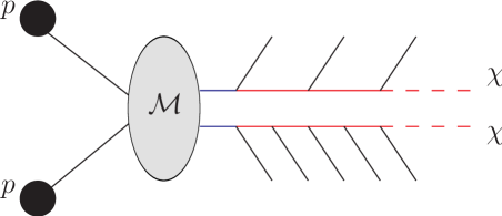
The second set of challenges we need to face is intrinsic to a high energy hadron collider (see Fig 4.2). These are mainly due to the fact that the incoming hadrons are ‘bags’ of quarks and gluons and the high energy interacting partons radiate gluons before they interact, according to the parton branching picture we presented in section 2.2.3.4. Thus, processes are always associated with copious collinear initial-state radiation (ISR) which affects the longitudinal momentum components of particles. Moreover, it is not possible to measure the initial longitudinal (i.e. along the -axis, defined parallel to the detector’s beam pipe) components of the interacting partons in hadron colliders, since what is left of the colliding hadrons (the ‘remnants’) travels down the beam pipe and is not detected.111Note, however, that central exclusive production, in which the protons remain intact and forward detectors can be used to measure the -component of the central system, has been investigated. See, for example, [60]. But the issues are not only limited to ISR and our inability to measure the -components of incoming partons: secondary partonic interactions between the interacting hadrons also play an important role, contaminating the signal with soft particles. It is also worthwhile to note that since the LHC is destined to become a high-luminosity machine,222Here we refer to the instantaneous luminosity of a collider with bunched beams. If two bunches containing and particles collide with frequency and the beam profiles are characterised by and , the transverse beam profiles in the horizontal and vertical directions respectively, then the instantaneous luminosity is given by . The rate of events for a certain process of cross section is then given by [13]. secondary proton-proton interactions (or ‘pile-up’) are also expected to add soft particles to the events. Of course, one cannot forget the various experimental challenges due to beam halo, noise and so on.333See, for example, Ref. [61] for details of the expected performance of the ATLAS experiment at the LHC.
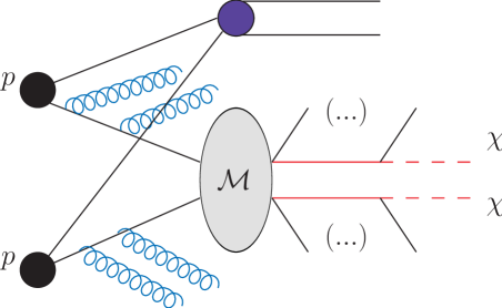
Several search variables of varying complexity and assumptions have been constructed to tackle the aforementioned issues. This is done, for example, either through cleverly defining variables that have discriminatory power against backgrounds, after cuts have been imposed to the event sample, or variables that are insensitive to QCD effects in certain ways.
Kinematic variables can be constructed in order to constrain the momenta of particles and hence search for new physics. They represent the first step in understanding the observations at hadron colliders, since they make very few assumptions about the details of the underlying physical model, such as the gauge groups, spins or couplings, providing model-independent, robust information [62]. The very simplest class of the kinematic variables are global inclusive variables, i.e. those that make use of all observed momenta, without hypothesising any particular structure of the final state. Since the longitudinal momentum of the hard process is unknown, transverse variables of this class have been generally investigated so far. Examples are the observed transverse energy , the missing transverse energy, , and their sum, . The distributions of these quantities can provide information on the energy scales of new processes such as supersymmetric particle production [63, 64, 65].
Although longitudinal components of final-state momenta are strongly influenced by ISR, they do contain information about the underlying hard process. Indeed, the amount of ISR emitted is determined by the energy scale of the subprocess. This has motivated several studies of global inclusive variables that contain longitudinal components, such as the and the total visible mass variables, which will be investigated in section 4.2.
Initial-state radiation also modifies the distributions of the products of the hard process. This effect has been studied in great detail for the processes of electroweak boson production, with the result that the transverse momentum and rapidity distributions of , and Higgs bosons at the Tevatron and LHC are predicted with good precision [66, 67, 68]. In contrast, the equivalent distributions have received little attention. In section 4.3 we will be investigating the distribution in vector boson production and Higgs boson production.
4.2 Effects of QCD radiation on global inclusive variables
4.2.1 Global inclusive variables
Global inclusive variables are easily defined with reference to Fig. 4.3, as found in [69]. We focus on a specific subprocess, formed by the interaction of two incoming partons from the hadrons (protons or anti-protons). The resulting final-state particles can be either visible, , or invisible, . The visible particles can originate either from the hard process itself or from ISR and can be jets, electrons, muons and photons. The invisible particles consist of SM neutrinos, which we take to be massless, and some new massive BSM particles, not necessarily of the same type. We can define, using the sum of the 4-momenta of all the visible particles, the total 3-momentum and the total energy . The only experimental information we possess about the invisibles is the total missing transverse momentum 2-vector, . Any global inclusive variable can be defined by using , components of and .
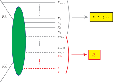
4.2.2 The variable
In Ref. [69] various global variables were investigated, including those that make use of longitudinal as well as transverse momentum components. The quantities studied included the total energy visible in the detector (as defined in section 4.2.1) and the visible invariant mass ,
| (4.1) |
where is the visible longitudinal momentum. In addition a new variable was introduced, defined as
| (4.2) |
where the parameter is a variable estimating the sum of masses of all invisible particles in the event:
| (4.3) |
The variable is simply the minimum value of the parton-level Mandelstam variable (the square of the partonic centre-of-mass energy) which is consistent with the observed values of the total energy , and in a given event. It was argued that the peak in the distribution of is a good indicator of the mass scale of new physics processes involving heavy particle production in the absence of ISR and multiple parton interactions. In Ref. [69] specific examples were given in , gluino pair-production and gluino-LSP associated production and the dependence on was also investigated.
It was also recognised that the effects of the ISR and the multiple parton interactions make this measurement impossible, since would measure the total energy of the full system, whereas the interest is on the energy of the hard scattering. In Ref. [70] an alternative approach was proposed, preserving the definition, but instead of using information from the calorimeters to construct the quantities , and , reconstructed objects were used. That means, objects that have been recognised via some algorithm as jets, muons, electrons or photons were used. This seems to recover some of the attributes of , but the distributions are not calculable analytically and hence we do not pursue this method here.
4.2.3 ISR effects without invisible particle emission
In the present section we examine the effects of ISR on global inclusive variables, first in an approximate fixed-order treatment, taking into account collinear-enhanced terms, and then in an all-orders resummation of such terms. We quantify the way the distributions of quantities that involve longitudinal momenta depend on the scale of the underlying hard subprocess and on the properties of the detector, in particular the maximum visible pseudorapidity . Initially, we ignore the effect of invisible final-state particles: we assume that all the final-state particles from the hard subprocess are detected. We will present the treatment of invisibles in section 4.2.5.
The Monte Carlo results presented in Ref. [69] show that the second term on the right-hand side of Eq. (4.2) is not strongly affected by ISR. The first term is intended to add extra longitudinal information about the hard subprocess, allowing a more reliable determination of its mass scale. The extra longitudinal information enters through the visible mass , and we therefore concentrate on this quantity.
4.2.3.1 Born approximation
In the Born (or leading-order) approximation, assuming that no beam remnants are detected, yields a perfect estimate of the centre-of-mass energy of the hard subprocess with no invisibles. For incoming partons with momentum fractions :
| (4.4) |
where is the hadron-hadron centre-of-mass energy, so that
| (4.5) |
where we have also defined the rapidity of the visible system, . The differential cross section for parton flavours is thus:
| (4.6) |
where are the relevant parton distribution functions for the incoming hadrons and is the hard subprocess cross section. Hence, at Born level we find
| (4.7) |
The parton distributions are sometimes given as , in terms of which we have
| (4.8) |
If the partonic cross section has a threshold or peak, indicating that the subprocess has a characteristic scale , then this is also manifest in the Born cross section (4.8) at , provided the relevant parton distributions are large enough for that subprocess to contribute significantly.
4.2.3.2 Quasi-collinear NLO correction
To examine the sensitivity of the above results to ISR, let us first compute the NLO contribution due to quasi-collinear gluon emission and the associated virtual corrections. Consider first the emission of a gluon from parton . If the emission angle , defined with respect to the beam direction in the lab frame, is large enough, say , the gluon enters the detector and contributes to . In the small-angle approximation we then have
| (4.9) |
where is the momentum fraction of parton before the emission, so that
| (4.10) |
The correction associated with a detected emission from parton is then:
| (4.11) |
where is the unregularised splitting function and we have neglected the running of for the moment.
On the other hand if the gluon misses the detector (), and are still given by Eq. (4.4), so the contribution is
| (4.12) |
Finally the associated virtual correction is the term that regularises the splitting function, which in this approximation is
| (4.13) |
Adding everything together gives a correction
Setting aside for the moment the possibility of splittings other than , the DGLAP evolution equation for is
| (4.15) |
where represents the scale at which the parton distribution is measured. Hence the correction may be written as
| (4.16) | |||||
Since , the first term represents a change of scale in the Born term. It replaces the reference scale in by the scale of the hard subprocess. The remaining terms give a correction
| (4.17) | |||||
In leading-log approximation the integration just gives a factor of . In the same approximation, we may set ,444Note that this is an approximation to the conventional definition of the pseudorapidity , consistent with the leading-long approximation. the maximum pseudorapidity seen by the detector. Note that this is a different quantity from , the true rapidity of the visible system. The correction associated with parton gives the same expression with and . Thus, defining
| (4.18) |
we have
Expressing this in terms of , as in Eq. (4.8),
Results for production at the LHC ( at TeV) with and are shown in Fig. 4.4. Leading-order MSTW parton distributions [71] were used. For simplicity we have taken . Recall that the simplifying assumption made here is that all decay products are detected, so the distribution vanishes below threshold. We see that there is a large negative NLO correction near threshold, followed by a broad positive peak.

To understand these qualitative features, consider the case , as in , and , so that . Then the NLO correction becomes simply:
| (4.21) |
The first term is positive-definite, contributes only above threshold, and diverges at threshold. It produces the broad positive peak. The second term is negative-definite, contributes around threshold, and has a divergent coefficient. It provides the sharp negative peak.
4.2.3.3 Resummation
By adding and subtracting the expression
| (4.22) |
in the integrand of Eq. (4.2.3.2) and comparing with Eq. (4.15), we see that the last line of that equation corresponds to a change of scale in the parton distributions, leading to
| (4.23) |
The above definition of includes the approximation in the evaluation of the PDFs, since they do not vary substantially with scale. To first order we can then write
| (4.24) | |||||
The interpretation of this result is simple: undetected ISR at angles less than , corresponding to scales less than , is absorbed into the structure of the incoming hadrons.
To resum the effects of gluons at angles greater than , consider first the real emission of such gluons from parton . In the quasi-collinear approximation these form an angular-ordered sequence, giving rise to a contribution to of
| (4.25) | |||||
where again we have made the identification and we are still neglecting the running of . The multiple convolution of the momentum fractions can be transformed into a product by taking Mellin moments. Defining
| (4.26) |
we have
| (4.27) |
where
| (4.28) |
Therefore defining correspondingly,
| (4.29) |
the contribution (4.25) to this quantity will be
| (4.30) |
which summed over gives
| (4.31) |
The corresponding virtual contributions give a Sudakov-like form factor,
| (4.32) |
and therefore the total contribution from parton is
| (4.33) |
where is the anomalous dimension,
| (4.34) |
being the regularised splitting function. Note that it is the virtual correction, introduced via the form factor in Eq. (4.32), that has regularised the splitting function. Parton gives a similar factor with in place of , so the result for the quantity (4.29) is simply
| (4.35) |
We can see as follows that this result is qualitatively correct. The anomalous dimensions are positive for small and negative for large . Thus, for , is enhanced relative to at small and suppressed at large . Now from the moment definition (4.26) small corresponds to large and vice versa. Hence the distribution of is suppressed at small and enhanced at large relative to the Born term, as observed in the Monte Carlo [69] and NLO results.
The emission of partons other than gluons is included by introducing the anomalous dimension matrix with elements given by
| (4.36) |
where is the regularised splitting function. Then
| (4.37) |
The corresponding generalisation of the evolution equation (4.15) is
| (4.38) |
Defining the moments of the parton distribution functions
| (4.39) |
we see that
| (4.40) |
with solution
| (4.41) |
Hence
| (4.42) |
where
| (4.43) |
showing that the evolution of the visible mass distribution is related to that of the parton distributions over the same range of scales.
Taking into account the running of the strong coupling in the evolution equation (4.38), Eq. (4.42) becomes
| (4.44) |
where
| (4.45) |
with the factor , coming from the QCD one-loop -function, Eq. (2.69), given in section 2.2.3.2, and
| (4.46) |
The running of will affect Eq. (4.37) similarly, giving
| (4.47) |
To invert the above we can write the following double convolution
| (4.48) |
where
| (4.49) |
In the above inversion, performed on the complex plane, the contour is formally defined to be to the right of all singularities of the integrand and runs parallel to the imaginary axis from to . We will be discussing the details of the inversion in section 4.2.4. It then follows from Eq. (4.45) that obeys an evolution equation like that of the parton distributions,
| (4.50) |
Putting everything together, the visible mass distribution is related to the hard subprocess cross section (in the absence of invisible final-state particles) as follows:
| (4.51) |
where the kernel functions and can be obtained by solving the evolution equation (4.50) with the initial condition that at or by directly using Eq. (4.49) to invert the Mellin transform. The results shown in this section use the former method whereas in section 4.2.5 results given by the latter method will be shown. Note also that the assumption that we had made in Eq. (4.23) has been alleviated in Eq. (4.51).
To verify that the integrated cross section is not affected by resummation, define and write Eq. (4.51) as
| (4.52) |
Now
| (4.53) |
and
| (4.54) |
Hence
| (4.55) |
in agreement with Eq. (4.6).
Resummed results corresponding to Fig. 4.4 are shown in Fig. 4.5. We see that the peak of the distribution has moved to much higher mass, beyond 1 TeV. This is due to multiple emission of ISR partons in the evolution of the initial state from the detection scale to the hard subprocess scale . As the value of is reduced, the range of evolution becomes smaller, less ISR is emitted, and the peak moves closer to the hard subprocess scale, as illustrated in Fig. 4.6. Results for higher values of the visible rapidity are shown in Fig. 4.7. The peak moves to lower mass as increases, as a consequence of the suppression of high masses by the rapid fall-off of the parton distributions at high . All the results shown in the present section have been obtained by solving the evolution equation (4.50) directly.
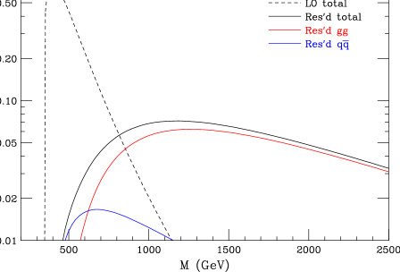


4.2.4 Mellin transform inversion
In the previous section we presented results using the direct integration of Eq. (4.50). In the following sections we will be using the inverse Mellin transform to calculate the kernel functions. We outline the procedure in this subsection.
Equation (4.49), sometimes called the Bromwich integral, defines the inverse of a Mellin transform. Formally, the contour on the complex -plane is to the right of all singularities in the integrand and runs parallel to the imaginary axis from to +. The formal contour is shown in Fig. 4.8 in blue dashes.
However, we often need to perform the inversion on the complex plane numerically. The formal contour turns out to be inappropriate for a numerical calculation. To see this, consider the parametrization of the contour passing through the point on the real axis: , where is a parameter which runs from to . Then the Bromwich integral becomes
| (4.56) |
The above expression will not converge numerically because of the oscillatory nature of the factor . In PDF evolution this is ameliorated by deforming the contour to contour , shown in Fig. 4.8 in purple dot-dashes. If there are no singularities in the integrand in the region , we expect the result of the integration not to change by the deformation. This is indeed the case for all the functions we will be considering. The contour can be parametrized as where is a constant related to the slope of the straight lines as shown in Fig. 4.8. It is easy to see that if , then a damping term of the form is introduced in the integrand and hence numerical convergence can be achieved. The contour is usually used to evolve parton density functions [72], according to Eq. (4.44).
However, in the case of the evolution kernels , the linear contour does not provide sufficient accuracy to reproduce the function from its transform. This is due to its inability to accurately invert a constant function to the correct analytic result, a delta function. This implies that the inversion does not reproduce the necessary initial condition, . A numerically more accurate contour is available in the literature, used in the so-called ‘Fixed-Talbot algorithm’. This contour, is shown in solid red in Fig. 4.8. It has the form , where is a parameter which we will set to during the computation, being the required precision in number of decimal digits, a value derived from numerical experiments. The contour is related to the ‘steepest descent’ path for a certain class of functions. For further details on its origin and accuracy see Ref. [73]. A comparison of the resulting ‘delta’ functions obtained by using and can be seen in Fig. 4.9. It is obvious that the function obtained by using behaves much more like a delta function.
We first rewrite the evolution kernel in a more convenient basis:
| (4.57) |
where is the matrix of eigenvectors of and is the diagonal matrix of its eigenvalues. This is equivalent to using, implicitly, the singlet and non-singlet basis [10].
As a test of the evolution using Mellin inversion, we used the contour to evolve -quark and gluon PDFs from a starting scale of to . The form of at was extracted directly from the the leading-order MSTW parton distributions [71] and the evolved results at were compared to the actual values given by the MSTW PDFs. The results are shown in Fig. 4.10, exhibiting good agreement for most of the range of values of . The discrepancy at high is due to the difference in treatment of as .
4.2.5 ISR effects including invisible particle emission
Suppose now that an invisible 4-momentum is emitted from the hard subprocess. If we define the total lab frame 4-momentum of the incoming partons and as , then
| (4.58) |
and the visible 4-momentum will be given by . By definition, the visible mass is then
| (4.59) |
Equation (4.59) demonstrates the interplay between two effects: on one hand ISR increases the ‘true’ scale of the hard process , to the ‘apparent’ scale by contaminating the detector with extra particles, and on the other hand the invisible particle emission decreases by the loss of particles. In the case of gluino pair-production both effects are equally important, as we will show.
Substituting from Eq. (4.58) in Eq. (4.59) and defining , we obtain
| (4.60) |
where represents the total invariant mass of the invisibles, .
The momenta are defined in the lab frame, relative to which the centre-of-mass frame of the hard subprocess is boosted by an amount defined by the momentum fractions and of the partons entering the subprocess. This implies that the transform as
| (4.61) |
where , defined in terms of the invisible momentum, , in the centre-of-mass frame of the hard subprocess. Substituting the expressions of Eq. (4.61) in Eq. (4.60), we find an expression for the visible invariant mass:
| (4.62) |
where we have defined and used . We may now solve Eq. (4.62) for to obtain in terms of :
| (4.63) |
The above expression for the hard subprocess scale now becomes the argument of the parton-level cross section, in Eq. (4.51):
| (4.64) |
The functions , which are related to the invisible particle 4-momenta, remain to be determined. The visible system rapidity, , is also modified by the presence of invisible particles as
| (4.65) |
and therefore Eqs. (4.18) for become:
| (4.66) |
The kinematic constraints restrict to be greater than the threshold energy squared for the process and the true invariant mass, , to be greater than the visible invariant mass, . These result in the following two constraints for :
| (4.67) |
4.2.5.1 Single-invisible decays
The benchmark scenario for a single invisible decay originating from the hard process is production in which one of the two tops decays into (hadronic) and the other into (semi-leptonic), the neutrino comprising the missing 4-momentum. Excluding the proton remnants, we assume that all other particles within the pseudorapidity coverage are detected. We will refer to the neutrino as the invisible particle and the as the intermediate particle in the case, but the treatment is readily applicable to the gluino case where the invisible particle is the and the intermediate particle is a squark (treated in section 4.2.5.2).
To calculate the functions and obtain , we need to calculate the neutrino 4-momentum in the hard process frame. This is done by choosing the neutrino 4-momentum in the frame of its parent and then applying two subsequent Lorentz boosts: one going from the frame to the top frame, and one from the top frame to the hard process frame. The decay chain is shown in Fig. 4.11. Each of these boosts involves two angular variables which originate from the ‘decay’ of the parent particle. Hence the 4-momentum of the neutrino may be written as
| (4.68) |
where the ’s are Lorentz boost matrices and where quantities with a hat refer to the hard process frame, quantities with a tilde refer to the top frame and quantities with a bar refer to the frame. The angles and represent the usual polar angles, defined with respect to the direction of the ‘sister’ particle (see Fig. 4.11). For example, in the case , where the was produced from the top decay along with a bottom quark, the angles are defined with respect to the direction of motion of the quark in the frame. The two boost vectors have magnitudes given by (), the ratio of the parent 3-momentum magnitude and its energy. The boosts, as well as the magnitude of the invisible particle 4-momentum, can be obtained by considering the kinematics in each frame as:
| (4.69) | |||
where is the unit vector in spherical polar coordinates in the appropriate frame and , are the and top quark masses respectively. The 4-vector , and hence the functions , are calculated by . Evidently, the functions are functions of , giving an implicit equation for . To make this more explicit, we rewrite Eq. (4.63):
| (4.70) |
and analogously for Eq. (4.2.5), where represents the set of all angular variables. In the present case but for multiple invisible particles it will also be a function as indicated.
Equation (4.70) needs to be solved numerically for each set () in the region , where is the square of the proton centre-of-mass energy, along with the restriction that the visible invariant mass should be lower than the ‘true’ invariant mass, . The numerical solution was found using the Van Wijngaarden-Dekker-Brent method [74, 75], a bracketing method for finding roots of one-dimensional equations. Since is not uniquely determined for each , different values of the ‘true’ centre-of-mass energy contribute to the cross section. Note that not all possible configurations () are kinematically allowed to contribute to the cross section at and hence some configurations do not yield roots of Eq. (4.70). Once is obtained, the parton-level cross section for the hard process partons, , is calculated. This result is then multiplied with the parton density functions for the incoming partons, , and the kernels for evolution from incoming partons and to hard process partons and ( and ). We then integrate over all possible values of and , according to Eq. (4.64). Finally, to obtain the full resummed result we have to integrate over the distribution of the angular variables .
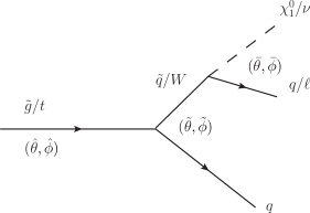
Notice that the visible invariant mass distribution becomes non-zero below the threshold for production, , owing to the loss of invisible particles.
4.2.5.2 Double-invisible decays
We now turn to the case where both particles produced in the hard process decay invisibly. For illustration we refer to sequential decays of the gluino: . Although this decay mode is generally not the dominant one, it is useful for illustration of the procedure. We extend the treatment given in the semi-leptonic/hadronic top case by writing out functions related to the two invisible particle 4-momenta in the decay chain (which we call and ):
| (4.71) | |||
| (4.72) |
where the primed quantities now distinguish between the two invisibles. Since both of these 4-vectors are defined in the hard subprocess frame, we simply have
| (4.73) |
The rest of the treatment is identical to the case for one invisible particle: an implicit equation has to be solved to obtain for each (, , ) set and then an integral over is taken to obtain the resummed result.
4.2.5.3 Angular distributions
The distributions of the angular variables , appearing in the treatment of invisibles given in the previous sections, are process-dependent. They represent the angles at which the daughter particle is emitted in the frame of the parent particle. We investigated the angular distributions using H ERWIG++ version 2.4.0 and subsequently used the results in calculating the functions. The results for SPS1a gluino pair-production are shown in Fig. 4.12, where the uniform distributions are shown for comparison (red horizontal line). Figure 4.13 shows the distributions as obtained for top pair-production. The neutrino angle in the frame is also compared to the analytic calculation. As expected, all the angles, in both cases, were found to be uniform (not shown). The form of all the distributions can be justified using general spin considerations:
-
:
The angular distribution of the angle at which the fermions are produced in the hard process frame is expected to have the form , where is a process-dependent constant.
-
:
The angle , is defined between the direction of the daughter boson ( or ) with respect to the direction of polarisation of the parent ( or ). The angular distribution for a spin-up fermion parent is then given by [76]
(4.74) where is a constant and is the modulus of the polarization of the parent. Since the production processes for both and are parity-conserving, there is also an equal spin-down () contribution to the total distribution with the sign of reversed. This results in a uniform distribution for .
Figure 4.12: Monte Carlo results for the gluino pair-production decay chain angles. From left to right: the production angle of the gluino in the hard process frame, the angle of the outgoing squark in the gluino frame and the angle of the outgoing neutralino in the squark frame. The uniform distributions are shown for comparison. -
:
In gluino pair-production, the decay products of the squark, , which is a scalar, are uniformly distributed in . In top pair-production, on the other hand, the decay is parity-violating and the distribution of is forward-backward asymmetric in the frame [10]. The angle (sometimes called , see e.g. [77]) can be used experimentally to infer helicity information on the . The distribution may be written as
where , and are the probabilities for left-handed, right-handed and longitudinal helicities of the in top quark decay respectively. The SM predictions, , yield the blue solid curve shown on the right in Fig. 4.13.
The spins of the two produced fermions (tops or gluinos) are correlated and this may cause a degree of correlation between the distributions of particles in the decay chains. We investigated whether these correlations play an important role in the calculation of the invisible particle effects on the visible mass. By comparing the invariant mass distributions with and without the spin correlations in the Monte Carlo we concluded that the effect is small in both top and gluino pair-production and can be safely neglected.
4.2.6 Results
We present the resummed distributions obtained for and production according to Eq. (4.64). All results are for the LHC at design energy, i.e. collisions at TeV. We have integrated over the visible system rapidity, , in the range . We first compare our results to those obtained using the H ERWIG++ event generator at parton level (i.e. no hadronization or underlying event) and excluding the proton remnants.555We verified, using the event generator, that the contribution of the proton remnants to the total invariant mass in the considered rapidity range is negligible. In sections 4.2.6.3 and 4.2.6.4 we examine the effects of hadronization and the underlying event. Parton-level top and gluino pair-production cross section formulae are given in appendix B. The PDF set used both in the resummation calculation and H ERWIG++ is the MRST LO** (MRSTMCal) set [78, 79].
4.2.6.1 Top quark pair-production
We present resummed results in comparison to Monte Carlo for Standard Model production, where we include particles with maximum pseudorapidity . In Figs. 4.14 and 4.15 we show separate results for combinations of hadronic and semi-leptonic decays of the top, leading to zero, one or two invisible neutrinos from the hard process. The effect of the invisibles in both the fully semi-leptonic case and the hadronic/semi-leptonic case are small compared to the effects of hadronization, to be discussed in section 4.2.6.3. The differences between the Monte Carlo and resummed curves in Figs. 4.14 and 4.15 may be attributed to sensitivity to the behaviour of the PDFs and parton showering at low scales, since can be as low as in the case of production, and the precise definition of in terms of .
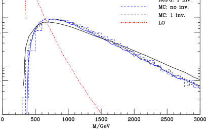
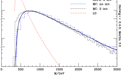
4.2.6.2 Gluino pair-production
We focus on the SPS1a point [80], which has gluino and lightest neutralino masses and respectively (and see table 4.1 for the squark masses). For simplicity we set the squark mass in the invisible particle treatment to . We also present results for a modified SPS1a point, with . In this process only the two-invisibles case is realistic, but for comparison we also show results for no invisibles, i.e. imagining that the two lightest neutralinos are also detected.
| Particle | Mass (GeV) | Particle | Mass (GeV) |
|---|---|---|---|
| 604.5 | 570.7 | ||
| 97.0 | 547.9 | ||
| 562.3 | 515.3 | ||
| 548.2 | 547.7 | ||
| 570.7 | 400.7 | ||
| 547.9 | 586.3 |
When , there is fairly good agreement between the Monte Carlo and resummation predictions in both the two-invisibles and no-invisibles cases, and for both gluino masses, as shown in Figs. 4.16 and 4.17, where one should compare the dashed histograms (Monte Carlo) to the solid curves of the same colour (resummation).
The shift in the peak of the visible mass distribution in going from no to two invisibles is much larger than that in top pair-production, amounting to 600-700 GeV, roughly independent of and the gluino mass. This results mainly from the higher masses of the intermediate particles in the decays ( GeV vs. GeV), which implies a higher energy release, rather than the masses of the invisible particles themselves ( GeV vs. ).
One of the assumptions of the resummation is that all the visible hard process decay products are detected, which is not true when the maximum pseudorapidity is restricted to lower values. When in the Monte Carlo analysis, a significant number of hard process particles begin to be excluded and hence the curves shift to lower values compared to the resummed predictions. Figure 4.18 shows the rapidity distribution of the decay products of the gluino at parton level for . For the case shown, cuts of and correspond to exclusion of, respectively, 0.002%, 1.1%, 7.5% and 20.0% of the gluino decay products from the detector. The effect of this appears in Figs. 4.19 and 4.20, where the Monte Carlo distributions are narrower and peak at lower masses than the resummed predictions. The variation between the resummed and 1.4 curves is smaller than that between and 3, since they correspond to smaller differences in .
The heavy and light gluino scenarios exhibit similar behaviour when varying the pseudorapidity coverage and the number of invisibles, showing the lack of dependence of the resummation on the mass of the pair-produced particle. The sensitivity to low-scale PDF behaviour and showering is reduced compared to the case since we are considering higher centre-of-mass energies, with the lowest possible now being of the the order . The position of the curves is again also sensitive to the precise definition of in terms of .
| (GeV). | MC (GeV) (0 inv./2 inv.) | Resum. (GeV) (0 inv./2 inv.) | |
|---|---|---|---|
| 604.5 | 5 | 2280/1560 | 1785/1620 |
| 604.5 | 3 | 1680/1080 | 1593/1204 |
| 604.5 | 2 | 1440/840 | 1497/1204 |
| 604.5 | 1.4 | 1380/660 | 1497/1204 |
| 800.0 | 5 | 2820/2100 | 2569/1870 |
| 800.0 | 3 | 2220/1620 | 2128/1684 |
| 800.0 | 2 | 1920/1380 | 1865/1683 |
| 800.0 | 1.4 | 1740/1140 | 1865/1683 |
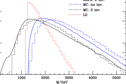
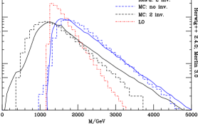
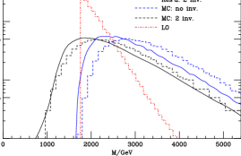
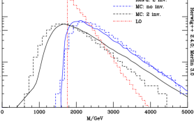

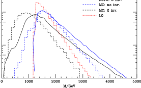
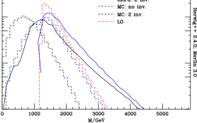
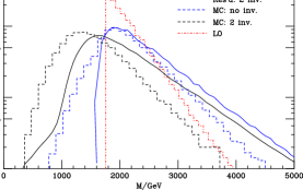
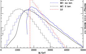
Table 4.2 shows a summary of the peak positions for all cases and different pseudorapidity cuts. For the higher values of , the agreement between the Monte Carlo and resummation is satisfactory. There is a large difference in the peak positions for no invisibles and , but this is mainly due to the broad shape of the peak in this case, while the overall distributions agree better. For there is a growing discrepancy, especially for the realistic case of two invisibles, due to the loss of particles coming from the hard process.
4.2.6.3 Hadronization effects
We have assumed that ISR partons emitted at pseudorapidities above do not contribute to the visible invariant mass. This would be true if the hadronization process were perfectly local in angle. However, as a result of hadronization high rapidity ISR partons can produce lower rapidity hadrons and thus ‘contaminate’ the detector and shift the visible mass to higher values.
As we have already discussed in section 3.2.3, the hadronization model employed in the H ERWIG++ Monte Carlo is a refinement of the cluster model. The model involves clustering of partons into colour-singlet objects that decay into hadrons, resulting in a smearing of the pseudorapidity distribution which causes the increase in the visible mass described above. The effect is shown in Fig. 4.21 for gluino and top pair-production (excluding the invisible particles from the hard process). The effect was found to be larger for production where the mass distribution is shifted significantly, whereas in gluino pair-production the shift is negligible.666This was found to dependent solely on the mass of the pair-produced particle, with a similar effect to the gluino case appearing if the top mass is increased to .
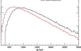
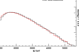
4.2.6.4 Underlying event
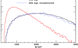
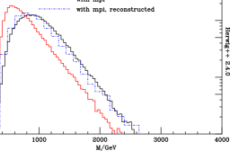
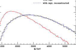
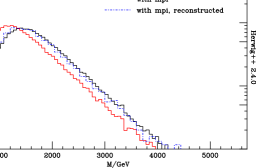
The underlying event, which we have discussed in section 3.2.2.5, is a further source of non-perturbative contributions to the visible mass. If represents the ‘hard’ visible 4-momentum studied in earlier sections and represents that due to the underlying event, the total visible mass is given by
| (4.76) | |||||
where we neglect transverse momentum associated with the underlying event. Thus, even if the visible invariant mass due to the underlying event is small, its effect on the overall visible mass may be enhanced through the last term on the right-hand side.
As we have already mentioned, the underlying event is simulated in H ERWIG++ by a multiple parton interaction model. In this model, for the rapidity ranges considered here, the underlying event is approximately process-independent and exhibits little correlation with the rest of the event. Therefore, to a good approximation, the distributions of the variables related to the underlying event, and , can be determined once and for all at each collider energy. The process-dependence comes primarily through the dependence on and , which can be calculated using the resummation formula given in Eq. (4.64). The overall visible mass distribution can then be obtained by convolution using Eq. (4.76).
The effects of including the underlying event in the visible mass distribution are shown in Figs. 4.22 and 4.23 for and gluino pair-production, respectively. The multiple parton interactions push the peak value to substantially higher masses. The shift amounts to about 250 GeV at and 1.2 TeV at , and is roughly process-independent. However, since the underlying event is approximately uncorrelated with the hard process, the visible mass distributions can be reconstructed well by the convolution procedure outlined above, as shown by the blue dot-dashed curves in Figs. 4.22 and 4.23. The distributions for the underlying event, , used to obtain Figs. 4.22 and 4.23, are shown in Fig. 4.24. These features of the underlying event will need to be validated by LHC data on a variety of processes. Accurate modelling of the underlying event is important for practically all aspects of hadron collider physics.
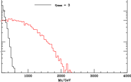
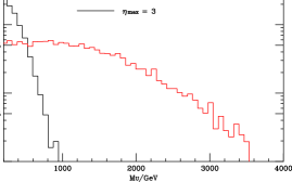
4.2.7 Conclusions
We have presented detailed predictions on the total invariant mass of the final-state particles registered in a detector, as a function of its pseudorapidity coverage by considering the effects of QCD initial-state radiation, first in the quasi-collinear NLO approximation and then in an all-orders resummation of the collinear-enhanced terms. This quantity provides the dominant contribution to many global inclusive observables such as the new variable (Eq. (4.2)), which can provide information on the energy scales of hard processes. We have extended the resummation method presented to include the effects of invisible particle emission from the hard process. We have considered the case of one or two invisible particles and presented results for Standard Model top quark pair-production and SPS1a gluino pair-production, obtained using a numerical Mellin moment inversion method.
In the case of production the invisible particles are neutrinos from boson decays and their effect on the visible invariant mass distribution is small, even when both decays are leptonic. This is mainly a consequence of the small boson mass compared to the overall invariant mass, rather than the negligible neutrino mass. For gluino pair-production the invisibles are a pair of massive LSPs from squark decays. The LSP mass is again small compared to the overall invariant mass, but the squark masses are not, leading to a substantial downward shift in the visible mass distribution, of the order of the squark mass. In both cases the resummed predictions are in fair agreement with Monte Carlo estimates of the position of the peak in the distribution, provided the pseudorapidity range covered by the detector is large enough (). For , the difference between the Monte Carlo prediction and resummed predictions is of the order of 100 GeV for both the heavy and light gluino SPS1a points. The agreement becomes worse when the pseudorapidity range is restricted, due to particle loss from the hard process. Table 4.2 shows the positions of the peaks of the distributions for the Monte Carlo results from H ERWIG++ and the resummation.
These comparisons were made with Monte Carlo visible mass distributions at parton level. We found that non-perturbative effects, especially the underlying event, tend to shift the invariant mass distributions to significantly higher values than expected from a purely perturbative calculation. According to the underlying event model used in H ERWIG++ , the shift amounts to about 250 GeV at and 1.2 TeV at . This effect is also expected in other observables sensitive to longitudinal momentum components, such as . However, in the model found in H ERWIG++ version 2.4.x, the underlying event is only weakly correlated with the rest of the event and hence its effects can be determined once and for all at each collider energy. The modelling of the underlying event is an important feature of the Monte Carlo programs that needs to be validated by comparison with experiment. Once this has been done, a wide range of global inclusive observables, including the visible invariant mass, will be reliably predicted and useful for establishing the scales of contributing hard subprocesses.
It is important to note that recent UE results from the LHC experiments have shown that the model present in H ERWIG++ 2.4.x does not describe the data adequately [81]. A more recent version of the event generator, 2.5.0 [53], which includes a model for colour reconnection, an extension of the cluster model of hadronization, achieves major improvements in the description of the UE LHC data.
4.3 Resummation of in vector boson and Higgs boson production at hadron colliders
QCD radiation from incoming partons changes the distributions of the products of the hard process. This effect has been studied in great detail for the processes of electroweak boson production, with the result that the transverse momentum and rapidity distributions of , and Higgs bosons at the Tevatron and LHC are predicted with good precision.777See [66, 67, 68] and references therein. The predictions for the transverse momentum () distributions in particular include resummation of terms enhanced at small to all orders in , matched with fixed-order calculations at higher values. The transverse momentum of the boson arises (neglecting the small intrinsic transverse momenta of the partons in the colliding hadrons) from its recoil against the transverse momenta of the radiated partons: , where:
| (4.77) |
The resummation of enhanced terms therefore requires a sum over emissions subject to the constraint (4.77), which is most conveniently carried out in the transverse space of the impact parameter Fourier conjugate to :
| (4.78) |
One then finds that the cumulative distribution in contains terms of the form , where is the scale of the hard process, set in this case by the mass of the electroweak boson, and . These terms, which spoil the convergence of the perturbation series at large , corresponding to small , are found to exponentiate [82, 83, 84, 85, 86, 87, 88]: that is, they can be assembled into an exponential function of terms that are limited to . This resummation procedure improves the convergence of the perturbation series at large values of and hence allows one to extend predictions of the distribution to smaller values.
Together with its vector transverse momentum , every emission generates a contribution to the total hadronic transverse energy of the final state, , which, neglecting parton masses, is given by
| (4.79) |
To first order in (0 or 1 emissions) this quantity coincides with , but they differ in higher orders. In particular, at small there is the possibility of vectorial cancellation between the contributions of different emissions, whereas this cannot happen for the scalar . Thus the distribution of vanishes faster at the origin, and its peak is pushed to higher values. To resum these contributions at small , one should perform a one-dimensional Fourier transformation and work in terms of a ‘transverse time’ variable conjugate to :
| (4.80) |
Since the matrix elements involved are the same, one finds a similar pattern of enhanced terms at large as was the case for large : terms of the form with , which arise from an exponential function of terms with . Evaluation of the exponent to a certain level of precision (leading-logarithmic, LL, for , next-to-leading, NLL, for , etc.) resums a corresponding class of enhanced terms and extends the validity of predictions to lower values of .
The resummation of in this way has received little attention since the first papers on this topic, over 20 years ago [89, 90, 91]. This is surprising, as most of the effects of QCD radiation from incoming partons mentioned above depend on this variable rather than . A possible reason is that, unlike , also receives an important contribution from the underlying event, which is thought to arise from secondary interactions between spectator partons, as discussed in section 3.2.2.5. At present this can only be estimated from Monte Carlo simulations that include multiple parton interactions (MPI). Nevertheless it is worthwhile to predict as accurately as possible the component coming from the primary interaction, which carries important information about the hard process. For example, we expect the distributions in Higgs and vector boson production to be different, as they involve primarily gluon-gluon and quark-anti-quark annihilation, respectively. Accurate estimates of the primary distribution are also important for improving the modelling of the underlying event.
In the present section we extend the resummation of in vector boson production to next-to-leading order (NLO) in the resummed exponent, parton distributions and coefficient functions, and present for the first time the corresponding predictions for Higgs boson production. In section 4.3.1 the resummation procedure is reviewed and extended to NLO; results on the resummed component are presented in section 4.3.2. This component alone is not expected to describe the region of larger values, of the order of the boson mass; in section 4.3.3 we describe and apply a simple procedure for including the unresummed component at order . Section 4.3.4 presents distributions generated using the parton shower Monte Carlo programs HERWIG version 6.510 [92] and H ERWIG++ version 2.4.0 [46], which are compared with the analytical results and used to estimate of the effects of hadronization and the underlying event. Our conclusions are summarised in section 4.3.5. Appendix D.1 gives mathematical details of a comparison between the resummation of the transverse energy and transverse momentum and appendix D.2 shows results for the LHC at lower centre-of-mass energy ().
4.3.1 Resummation method
4.3.1.1 General procedure
Here we generalise the results of Ref. [90] to NLO resummation. The resummed component of the transverse energy distribution in the process at scale takes the form:
| (4.81) | |||||
where is the parton distribution function (PDF) of parton in hadron at factorisation scale , taken to be the same as the renormalisation scale here. In what follows we use the renormalisation scheme. As mentioned earlier, to take into account the constraint that the transverse energies of emitted partons should sum to , the resummation procedure is carried out in the domain that is Fourier conjugate to , using Eq. (4.80). The transverse energy distribution (4.81) is thus obtained by performing the inverse Fourier transformation with respect to the transverse time, . The factor is the perturbative and process-dependent partonic cross section that embodies the all-order resummation of the large logarithms . Since is conjugate to , the limit corresponds to .
As in the case of transverse momentum resummation [93], the resummed partonic cross section can be written in the following universal form:
| (4.82) | |||||
Here is the cross section for the partonic subprocess , where (the quark and the anti-quark can possibly have different flavours ) or . The term is the quark or gluon Sudakov form factor. In the case of resummation, this takes the form [90, 91]:
| (4.83) |
with or . The functions , as well as the coefficient functions in Eq. (4.82), contain no terms and are perturbatively computable as power expansions with constant coefficients:
| (4.84) | |||||
| (4.85) | |||||
| (4.86) |
Thus a calculation to NLO in involves the coefficients , , , and . All these quantities are known for both the quark and gluon form factors and associated coefficient functions. Knowledge of the coefficients leads to the resummation of the leading logarithmic (LL) contributions at small , which in the differential distribution are of the form where . The coefficients give the next-to-leading logarithmic (NLL) terms with , and give the next-to-next-to-leading logarithmic (N2LL) terms with , and gives the N3LL terms with . With knowledge of all these terms, the first term neglected in the resummed part of the distribution is of order .
In general the coefficient functions in Eq. (4.82) contain logarithms of , which are eliminated by a suitable choice of factorisation scale. To find the optimal factorisation scale, we note that, to NLL accuracy,
| (4.87) |
where , being the Euler-Mascheroni constant. See appendix D.1 for a derivation. The effective lower limit of the soft resummation becomes , and the parton distributions and coefficient functions should be evaluated at this scale. However, evaluation of parton distribution functions at an imaginary scale using the standard parametrizations is not feasible. We avoid this by noting that
| (4.88) |
where is the DGLAP evolution kernel, also used in section 4.2.3.3 (see, e.g. Eq. (4.54)). Therefore:
| (4.89) |
where the evolution kernel is given to NLO by
| (4.90) |
where is the leading-order DGLAP splitting function. Similarly, in the coefficient functions we can write in terms of using the definition of the running coupling, given in section 2.2.3.2:
| (4.91) |
where , so that
| (4.92) |
Furthermore, as the expressions (4.81) and (4.82) are convolutions, we can transfer the extra terms from (4.89) into the coefficient functions to obtain
| (4.93) | |||||
where
| (4.94) |
Now the lowest-order coefficient function is of the form:
| (4.95) |
and therefore
| (4.96) |
Putting everything together, we have
| (4.97) |
where, taking all PDFs and coefficient functions to be evaluated at scale ,
| (4.98) |
To write (4.97) as an integral over only, we note from (4.89) and (4.90) that when , to NLO the real parts of and are unchanged but the imaginary parts change sign. All other changes in (4.98) are beyond NLO. Thus, writing
| (4.99) |
is symmetric with respect to and is antisymmetric. Defining
| (4.100) |
we therefore obtain
| (4.101) | |||||
where, inserting (4.95) and (4.96) in (4.98) and defining , we have to NLO,
| (4.102) |
It will be more useful to write, for example,
| (4.103) |
This makes it more straightforward to interpret the plus prescription, which appears in some splitting functions, as
| (4.104) | |||||
We show in appendix D.1 that the results of resummation of the scalar transverse energy are identical to those of the more familiar resummation of vector transverse momentum at order , as they should be since at most one parton is emitted at this order.
The transverse energy computed here is the resummed component of hadronic initial-state radiation integrated over the full range of pseudorapidities . In Ref. [90] the distribution of radiation emitted in a restricted rapidity range was also estimated. This was done by replacing the lower limit of integration in Eqs. (4.3.1.1) by , i.e. assuming that radiation at does not enter the detected region. This is justified at the leading-logarithmic level, where and the scale dependence of the parton distributions and coefficient functions in Eq. (4.98) can be neglected. Then when the form factor is replaced by unity and Eq. (4.97) correctly predicts a delta function at times the Born cross section. However, this simple prescription cannot be correct at the NLO level, where the -dependence of the scale must be taken into account. Therefore we do not consider the distribution in a restricted rapidity range here.
It is worth noting at this point, an existing related resummation of a variable called the ‘beam thrust’, essentially defined as the weighted by [94].
4.3.1.2 Vector boson production
One of the best studied examples of resummation is in vector boson production through the partonic subprocess ( or ):
| (4.105) |
where, at lowest order,
| (4.106) |
with the appropriate CKM matrix element and the vector and axial couplings to the Z0. The coefficients in the quark form factor are [86, 95]:
where is the Riemann -function , , , is the number of light flavours, and:
| (4.108) |
The above expression for is in a scheme where the subprocess cross section is given by the leading-order expression (4.105). In the same scheme the NLO coefficient functions are [95, 96]:
| (4.109) |
where the second line defines . The corresponding splitting functions are:
| (4.110) |
Equations (4.3.1.1)–(4.104) therefore give
4.3.1.3 Higgs boson production
In the case of Higgs boson production the corresponding LO partonic subprocess is gluon fusion, , through a massive-quark loop:
| (4.112) |
where in the limit of infinite quark mass:
| (4.113) |
The coefficients in the gluon form factor are [97, 98, 99]:
Here again, the above expression for is in a scheme where the Higgs boson subprocess cross section is given by the leading-order expression (4.112). In the same scheme the NLO coefficient functions are [100]:
| (4.115) |
The corresponding splitting functions are:
| (4.116) |
Equations (4.3.1.1)–(4.104) therefore give
| (4.117) | |||||
where .
4.3.2 Resummed distributions
4.3.2.1 Vector boson production
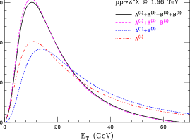
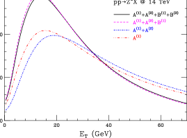
Figure 4.25 shows the resummed component of the transverse energy distribution in boson production at the Tevatron ( at TeV) and LHC ( at TeV).888Results for at TeV are given in appendix D.2. For all calculations, we use the MSTW 2008 NLO parton distributions [71]. The different curves show the effects of the subleading coefficients (4.3.1.2) in the quark form factor. We see that while has a large effect (the difference between the blue and magenta curves), the effects of the other subleading coefficients are quite small.
The peak of the resummed distribution lies at around GeV at the Tevatron, rising to GeV at the LHC. This is comfortably below , justifying the resummation of logarithms of in the peak region. However, at LHC energy the predicted distribution has a substantial tail at larger values of , indicating that the higher-order terms generated by the resummation formula remain significant even when the logarithms are not large. In addition, the LHC prediction does not go to zero as it should at small . However, this region is sensitive to the treatment of non-perturbative effects such as the behaviour of the strong coupling at low scales (we freeze its value below 1 GeV) and the upper limit in the integral over transverse time (we set where is the two-loop QCD scale parameter, set to 200 MeV here).
The resummed component for boson production looks very similar, apart of course from the overall normalisation, and therefore we do not show it here. Predictions with matching to fixed order will be presented in section 4.3.3.
4.3.2.2 Higgs boson production
Figure 4.26 shows the resummed component of the transverse energy distribution in Higgs boson production at the Tevatron and LHC, for a Higgs boson mass of 115 GeV. The effects of subleading terms in the gluon form factor (4.3.1.3) are more marked than those of the quark form factor discussed above. The distribution peaks at large values of , around 40 GeV at the Tevatron, rising to GeV at the LHC. This is due to the larger colour charge of the gluon. However, together with the large effects of subleading terms, it does make the reliability of the resummed predictions more questionable. Also in contrast to the vector boson case, the suppression at low and high is if anything too great, resulting in negative values below 16 GeV and above 120 GeV at Tevatron energy. We verified, by cutting-off the gluon PDFs at zero, that the negative values are due to the resummation and not due to the gluon PDF becoming negative at low values.
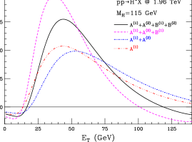
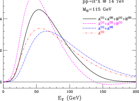
4.3.3 Matching to fixed order
The resummed distributions presented above include only terms that are logarithmically enhanced at small . To extend the predictions to larger we must match the resummation to fixed-order calculations. To avoid double counting of the resummed terms, the corresponding contribution must be subtracted from the fixed-order result.
We consider here only matching to first order in . To this order the distribution for has the form:
| (4.118) |
where and are constants (for a given process and collision energy) and the function is regular at . The terms involving and are already included in the resummed prediction, and therefore we have only to add the regular function to it to obtain a prediction that is matched to the result. This function is determined by fitting the prediction for to a linear function of at small , extracting the coefficients and , and then subtracting the enhanced terms in Eq. (4.118).
4.3.3.1 Vector boson production


The above matching procedure is illustrated for production at the Tevatron in Fig. 4.27. The fit to the logarithmically enhanced terms gives excellent agreement with the order- result out to around 20 GeV, confirming the dominance of such terms throughout the region of the peak in Fig. 4.25. The remainder function vanishes at small and rises to around 10 pb/GeV, falling off slowly at large . Consequently the matching correction to the resummed prediction is small and roughly constant throughout the region 40–100 GeV, as shown in Fig. 4.28.
As shown on the right in Fig. 4.28, the situation is similar at LHC energy: the matching correction is small, although in this case it is negative below about 40 GeV. The large tail at high and the bad behaviour at low , due to uncompensated higher-order terms generated by resummation, are not much affected by matching to this order.


The corresponding matched predictions for boson production are shown in Fig. 4.29. As remarked earlier, the form of the resummed distribution is very similar to that for boson production, and again the matching correction is small.
Note that at high the distributions should approximate the matched distributions, although this is not apparent in the figures.
4.3.3.2 Higgs boson production


Adopting the same matching procedure for Higgs boson production, we find the results shown in Figs. 4.30 and 4.31. The form of the matching correction is similar to that for vector bosons, but its effect is rather different. The roughly constant, then slowly decreasing, correction in the region 20–100 GeV is not small compared to the resummed result and therefore it raises the whole distribution by a significant amount throughout this region. This has the beneficial effect of compensating the negative values at low and high at Tevatron energy. However, it further enhances the high tail of the distribution at LHC energy. This, together with the relatively large correction in the peak region, casts further doubt on the reliability of the predictions in the case of Higgs boson production.
4.3.4 Monte Carlo comparisons
In this section we compare the resummed and matched distributions obtained above with the predictions of the parton shower Monte Carlo programs HERWIG [92] and H ERWIG++ [46].
Comparisons are performed first at the parton level, that is, after QCD showering from the incoming and outgoing partons of the hard subprocess. We say ‘incoming and outgoing’ because both programs apply hard matrix element corrections: in addition to the Born process, real emission hard subprocesses are included in phase space regions not covered by showering from the Born process.
After showering, the Monte Carlo programs apply a hadronization model to convert the partonic final state to a hadronic one. We show the effects of hadronization in the case of HERWIG only; those in H ERWIG++ are broadly similar since both programs use basically the same cluster hadronization model we described in section 3.2.2.3. The programs also model the underlying event, which arises from the interactions of spectator partons (see section 3.2.2.5) and makes a significant contribution to the hadronic transverse energy. In this case we show only the underlying event prediction of H ERWIG++ , since the default model used in HERWIG has been found to give an unsatisfactory description of Tevatron data. For an improved simulation of the underlying event, HERWIG can be interfaced to the multiple interaction package JIMMY [43], which is similar to the model built into H ERWIG++ .
4.3.4.1 Vector boson production
Figure 4.32 shows the comparisons for production at the Tevatron and LHC. The HERWIG predictions are renormalised by a factor of 1.3 to account for the increase in the cross section from LO to NLO. The H ERWIG++ results were not renormalised, because they were obtained using LO** parton distributions [78], which aim to reproduce the NLO cross section. We see that the parton-level Monte Carlo predictions of both programs agree fairly well with the matched resummed results above about 15 GeV, but H ERWIG++ generates a substantially higher number of events with low values of . A similar pattern is evident in the results on boson production, shown in Fig. 4.33. The effects of hadronization, shown by the difference between the blue and magenta histograms, are also similar for both vector bosons. They generate a significant shift in the distribution, of around 10 GeV at Tevatron energy and 20 GeV at LHC.
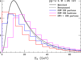
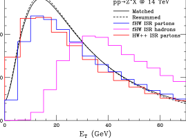
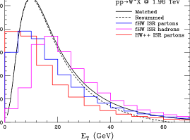
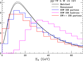
4.3.4.2 Higgs boson production
As may be seen from Fig. 4.34, the agreement between the resummed and parton-level Monte Carlo results is less good in the case of Higgs boson production than it was for vector bosons. Here we have renormalised the HERWIG predictions by a factor of 2 to allow for the larger NLO correction to the cross section. Then the Monte Carlo distributions agree quite well with each other but fall well below the matched resummed predictions. Fair agreement above about 40 GeV can be achieved by adjusting the normalisation, but then the Monte Carlo programs predict more events at lower . The effect of hadronization is similar to that in vector boson production, viz. a shift of about 10 GeV at the Tevatron rising to 20 GeV at the LHC, which actually brings the HERWIG distribution into somewhat better agreement with the resummed result.
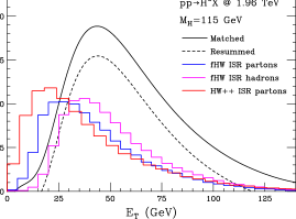
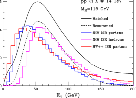
4.3.4.3 Modelling the underlying event
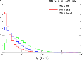
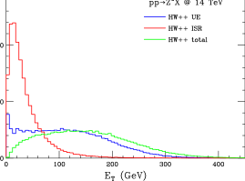
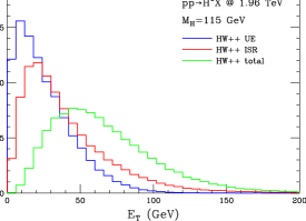
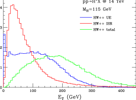
Figures 4.35 and 4.36 show the parton-level H ERWIG++ predictions for the distribution in and Higgs boson production, respectively, with the contributions from initial-state radiation (in red, already shown in Figs. 4.32 and 4.34), the underlying event (blue) and the combination of the two (green). As we have already seen in section 3.2.2.5, the underlying event is modelled using multiple parton interactions. Clearly it has a very significant effect on the distribution. However, this effect is substantially independent of the hard subprocess, as we have already found in section 4.2.6.4 when examining the total invariant mass, . This can also be seen from the comparison of the of the UE associated to different subprocesses in Fig. 4.37.
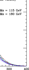
ERWIG++
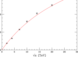
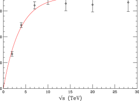
ERWIG++
We find that the probability distribution of the contribution of the underlying event in the H ERWIG++ Monte Carlo can be represented quite well by a Fermi distribution:
| (4.119) |
for which the normalisation, , is given by
| (4.120) |
The dependence of the ‘chemical potential’ and ‘temperature’ on the hadronic collision energy is shown in Fig. 4.38. The red curves show fits to the energy dependence of the form:
| (4.121) |
where the coefficients in the fits are , , , . Example fits for the LHC case, , are shown in Fig. 4.37.
4.3.5 Conclusions
We have extended the resummation of the hadronic transverse energy in vector boson production to next-to-leading order (NLO) in the resummed exponent, parton distributions and coefficient functions, and also presented for the first time the corresponding predictions for Higgs boson production. We have matched the resummed results to the corresponding predictions, by adding the contributions in that order which are not included in the resummation. In addition we have compared our results to parton shower Monte Carlo predictions and illustrated the effects of hadronization and the underlying event.
In the case of vector boson production, the resummation procedure appears stable and the parton-level results should be quite reliable. The leading-order mechanism of quark-anti-quark annihilation typically generates a moderate amount of transverse energy in initial-state QCD radiation. Consequently the effects of subleading resummed terms and fixed-order matching are small and the peak of the distribution lies well below the boson mass scale, where resummation makes good sense. The comparisons with Monte Carlo programs reveal some discrepancies but these are at the level of disagreements between different programs; in this case the resummed predictions should be more reliable (at parton level) than existing Monte Carlo programs. The programs suggest that the non-perturbative effects of hadronization and the underlying event are substantial. These effects can however be modelled in a process-independent way. We have suggested a simple parametrization of the contribution of the underlying event through the model given in the H ERWIG++ event generator. We stress once again, however, that recent UE results from the LHC experiments have shown that this model does not describe the data adequately [81], and as of version 2.5.0, H ERWIG++ includes an improved description [53] via a colour reconnection model. The effect of the improved model on the distributions remains to be investigated in future work.
The situation in Higgs boson production is not so good. The dominant mechanism of gluon fusion generates copious ISR and the effects of subleading terms and matching are large. The resummed distribution peaks at a value that is not parametrically smaller than the Higgs boson mass and the behaviour at low and high is unphysical before matching. The discrepancies between the matched resummed and Monte Carlo predictions are substantially greater than those between different programs, even allowing for uncertainties in the overall cross section. All this suggests that there are significant higher-order corrections that are not taken into account, either further subleading logarithms or unenhanced terms beyond NLO. It would be interesting (but very challenging) to attempt to extract such terms from the available NNLO calculations of Higgs boson production.
Chapter 5 New physics searches at hadron colliders
The original work in this chapter was done in collaboration with Oluseyi Latunde-Dada [4], Bryan Webber, Kazuki Sakurai and Ben Gripaios [5].
5.1 Introduction
The challenges present at hadron colliders have been discussed in section 4.1, where we emphasised that new physics signals can be difficult to observe and interpret. The difficulties arise due to multiple jets and/or leptons, the presence of invisible particles and the huge backgrounds that may potentially imitate the topology and kinematics of a signal of relatively low rate. It is thus extremely important to investigate the phenomenology of concrete models of new physics. At the same time, we need to ensure that we do not weaken our reach due to biases introduced by focusing on specific models. The strategies that we develop must allow us to explore the possibilities for generic new physics signatures, motivated by theoretically and experimentally plausible models. Furthermore, it is important for the observables that we construct to be well-defined and calculable so they can provide unambiguous information for the discovery of new physics and determination of its properties.
In this chapter we investigate two different new physics scenarios. In section 5.2 we present an investigation on a generic model that involves the production of a new heavy charged vector boson, called ( prime), essentially a heavy version of the standard model gauge boson. Such heavy bosons may arise from the breaking of a large symmetry group to the SM symmetry group, as excitations of the SM in models with extra dimensions, or as a composite particle in a strong dynamics theory. We study the interference effects of a with the SM and extend the treatment to next-to-leading order by using the MC@NLO and POWHEG methods described in section 3.3. We incorporate these features in a publicly available event generator and use this to examine the detection reach at the Tevatron and the LHC. In section 5.3 we examine a model that contains composite leptoquarks, particles that couple to leptons and quarks (as the name suggests), which may arise in strong dynamics theories. These couple primarily to the third generation of fermions, a feature motivated by a model of fermion mass generation which aims to solve the problem of flavour-changing neutral currents in theories where electroweak symmetry is broken via strong dynamics. We propose a general search strategy for discovery and mass reconstruction of leptoquarks.111It is interesting to mention that these two scenarios of new physics are not mutually exclusive. Both leptoquarks and heavy vector bosons may arise in the same model. This could be, for example, a strong dynamics theory that contains composite scalar particles, acting as leptoquarks, and composite vector particles, acting as ’s. In these models the bosons would also potentially couple preferentially to the fermions of the third generation.
5.2 NLO production of heavy charged vector bosons
5.2.1 Introduction
There exists a proliferation of theories which contain new heavy, electrically neutral or charged, gauge bosons referred to as and respectively. Both the and have been studied extensively and reviews can be found in [13] and [101] respectively. The study of this section focuses on bosons.
The new charged vector bosons may or may not have similar properties to the SM bosons, depending on the underlying theory. In particular they may have right-handed instead of left-handed couplings, may couple to new fermions, or may even be fermiophobic. Models which predict new charged vector bosons may be based on extensions of the electroweak gauge group, , for example to the gauge group [102], or groups that contain the electroweak symmetry, such as or [103]. Several models with extra dimensions contain bosons as Kaluza-Klein excitations in the bulk. Examples of these models include the Randall-Sundrum model (section 2.3.2.2) with bulk gauge fields [27] and Universal Extra Dimensions [26, 104]. Theories which break the electroweak sector via strong dynamics may also contain the as a composite spin-1 particle [105, 106].
Current Monte Carlo simulations of Drell-Yan-type production at hadron colliders rely mainly on leading-order matrix elements and parton showers. There exists no treatment of next-to-leading (NLO) QCD effects which simultaneously includes the interference effects for the . Here, we present the results of the event generator package Wpnlo [107] which improves the treatment of Drell-Yan production of heavy charged gauge bosons. We consider the interference effects with the Standard Model , which have been shown to provide valuable information [108], but have not been considered in experimental searches. We use the MC@NLO and POWHEG methods, discussed in section 3.3 to match the NLO QCD calculation to the parton shower, producing fully exclusive events using the H ERWIG++ event generator. Note that a similar implementation for the exists for the NLO MC@NLO event generator, which matches the complete NLO matrix elements with the parton shower and cluster hadronization model of the Fortran HERWIG event generator [109].
5.2.2 at leading order
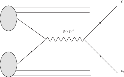
The reference model is based on the one which originally appeared in Ref. [110]. In the model described therein, sometimes referred to as the Sequential Standard Model, the magnitudes of the couplings to fermions are directly transcribed from the SM , i.e. it is a heavy copy of the SM . In the present treatment we allow both right- and left-handed couplings, respectively. In the case of right-handed couplings, we assume that the right-handed neutrinos are light compared to the , but not light enough for the boson to decay into them. The and couplings to fermions are given by
| (5.1) |
where is the Fermi coupling constant,222The constant is related to the weak coupling constant , which appears in Eq. (2.56), by . is the SM mass, are the coupling strengths of boson to leptons and quarks respectively, is the massive boson polarisation vector, and are the Dirac spinors for the fermions and is the unit matrix when are leptons and the CKM matrix, given in appendix C, when are quarks. The and represent the structure of the vector-axial vector (V-A) coupling of the bosons, where for the case we have , i.e. purely left-handed coupling. Using the above coupling to fermions, we show in appendix E.2 that the hadronic differential cross section for the process (Fig. 5.1) is given by
| (5.2) |
where is defined as the scattering angle between the -type quark and the outgoing neutrino (both being fermions) in the centre-of-mass frame, is the rapidity of the intermediate boson, is the ratio of the squares of the quark centre-of-mass energy to the proton centre-of-mass energy. and are functions of the quark centre-of-mass energy:
| (5.3) |
| (5.4) |
with
| (5.5) |
where can be either or and , are the mass and width of boson respectively. The functions that appear in the differential cross section are even or odd products of parton density functions for the relevant hadrons, given by
| (5.6) |
where is the parton density function for a quark in a hadron carrying hadron momentum fraction , in a collision in which the quark pair centre-of-mass energy squared is . The indices represent the type of the ‘left’ (travelling in the positive -direction) or ‘right’ (travelling in the negative -direction) hadrons respectively. This definition allows for easy modification of the cross section to the , by changing the PDFs accordingly. Analogous expressions can also be obtained for the case of (), by appropriately modifying the functions and taking . The width can be taken to be a free parameter in the reference model: the couplings of the to other gauge bosons or the Higgs boson are model-dependent.333An exception is the photon, for which the coupling is fixed by gauge invariance. Here we shall assume for illustration that the fermionic decay width444The fermionic decay width is thus also taken to be the lower bound on the total width. scales with the mass as (provided that , the mass of the top quark)555The factor of 4/3 comes from the extra decay channel that opens up when , e.g. . and that the tri-boson vertex is suppressed by a small mixing angle and can be neglected in the analysis.
5.2.3 interference
The narrow width approximation (NWA) is often used when discussing the production of new vector bosons. This approximation is usually claimed to be valid up to corrections. However, - interference effects can become important in certain regions even as the width , see for example [108], and as we also show below. Use of the NWA may thus lead to invalid conclusions, as pointed out in [111].
Interference effects arise because the Drell-Yan process can proceed either via an intermediate SM or a in the reference model. The matrix element squared for the process may be decomposed in the following way:
| (5.7) |
The last term, which contains the interference, depends on the functions and (Eqs. (5.3) and (5.4)). Here we discuss the function when studying interference effects, although the arguments for are equivalent. The function can be decomposed into pieces that arise individually due to the or the , and an interference piece:
| (5.8) |
where we have defined the interference term . Explicitly, this term may be written as
| (5.9) |
where we have set all the couplings and . It is evident that since for the SM , when we set then the interference term vanishes: . This implies that there is no interference for the case of the SM and a purely right-handed , and the square of the total matrix element for the process can be written as the sum of the squares of the individual matrix elements for the and :
| (5.10) |
It is simple to see why this is so: the and SM decay to final-state particles of different helicities, which are distinguishable, and hence the two processes cannot interfere. However, when and , i.e. both bosons possessing left-handed couplings, we have . In fact, by examining of the expression for (Eq. (5.3)), we observe that should be of the same order of magnitude as and . Figure 5.2 shows the variation of the interference term, as well as the and terms and , for the case . We observe that is negative (green, blue, purple) in the intermediate mass squared region . The total cross section in this region is less than the sum of the individual and cross sections. We note that the possibility of a reduced cross section is seldom considered in experimental searches. It is important to realise that the interference term is non-vanishing and comparable in magnitude to the other terms in even as , a clear indication that the narrow width approximation is not justified in the intermediate region.
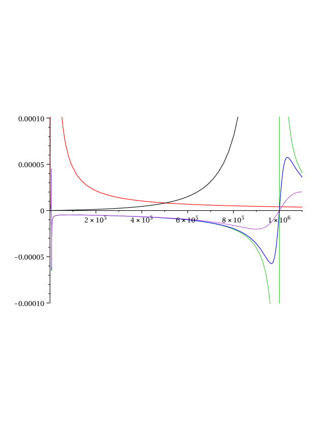
5.2.4 Extension to NLO
Next, we extend the simulation to NLO using the MC@NLO and the POWHEG methods. We briefly discuss their application to boson production. Full details of the application of the MC@NLO method to vector boson production can be found in section of Ref. [112]. Details of the application of the POWHEG method can be found in chapter of Ref. [59], where vector boson production is discussed in detail.
5.2.4.1 The MC@NLO method
The NLO cross section for the production of bosons can be written as a sum of two contributions:
| (5.11) |
where is the contribution from annihilation and is the contribution from the Compton subprocesses. In the modified minimal subtraction () factorisation scheme, these are:
| (5.12) | |||||
where is the Born differential cross section with the invariant mass and the rapidity of the vector boson. The are the NLO momentum fractions and are the Born momentum fractions with , if denotes the hadronic centre-of-mass energy. Also, and etc., with being the parton distribution function of parton .
Focusing on the annihilation process for the moment, if we introduce the variable
| (5.13) |
where is the scattering angle of the emitted parton in the partonic centre-of-mass frame, we can rewrite as an integral over and :
where is the real emission matrix element. Since we have subtracted this contribution from the total cross section, in the curly brackets we are left with the sum of the Born, virtual and QCD PDF correction contributions. Now we can define an infrared-safe observable whose NLO expectation value is given by
| (5.15) | |||||
where and are observables arising from hadronic final states generated from and starting configurations respectively. This however is not entirely correct because of double counting in the final states represented by which are already included in the states arising from . The solution to this is to subtract the parton shower contributions, which we denote , from the regions in which the parton shower contributes (the jet region ) and integrate the full matrix element in the hard emission region , left untouched by the shower. This gives for :
A similar functional can be generated for the Compton subprocesses. Events can then be generated in the different regions of phase space according to their contributions to the above integrals. These events are then interfaced with H ERWIG++ and showered. Full details of the algorithm for event generation can be found in [112].
5.2.4.2 The POWHEG method
The POWHEG method, as described in section 3.3, involves the generation of the hardest radiation from the parton shower according to the real emission matrix element and independently of the shower Monte Carlo generator used. If we introduce
| (5.17) |
where and are real emission matrix elements for annihilation and the Compton subprocesses respectively, we can write the cross section for the hardest gluon emission event as
| (5.18) |
The index runs over all quarks and anti-quarks. The subscript represents the Born variables, which in this case are the invariant mass and the rapidity of the boson, represents the radiation variables and , are the Born and real emission phase spaces respectively.
is the modified Sudakov form factor for the hardest emission with transverse momentum , as indicated by the Heaviside function in the exponent of Eq. (5.19):
| (5.19) |
where is the transverse momentum of the hardest emission relative to the splitting axis and in this case is given by
| (5.20) |
Furthermore:
| (5.21) |
is the sum of the Born (), virtual () and real () terms (with some counter-terms, ). The Born variables are generated with distribution , with the radiation variables of the first emission generated according to .
In the factorisation scheme, the contribution to the order- cross section for production is given by Eqs. (5.11) and (5.2.4.1). The function in Eq. (5.21) can then be written as a sum of finite terms using the subtraction method. Here we borrow the MC@NLO subtraction formula introduced in Eq. (5.2.4.1) and write the function as
where we have written the virtual and PDF corrections in terms of the real emission matrix elements and are the subtracted parton shower approximation terms in the H ERWIG++ jet regions. Note that the above prescription does not imply that the POWHEG method depends on the shower MC used. We have simply used the shower approximation terms to define a subtraction scheme for the definition of the NLO cross section.
The flavour of the event, the Born variables and , as well as the the radiation variables and are then generated according to the integrand in Eq. (5.2.4.2). The radiation variables are ignored, which amounts to integrating away these variables, leaving the Born variables distributed according to . The radiation variables are generated according to
| (5.23) |
Details of the algorithm used can be found in Ref. [59].
5.2.5 Experimental bounds
We provide a brief overview of direct and indirect searches for before presenting our results.
At the Fermilab Tevatron666The Tevatron is a proton-antiproton collider located at Fermilab, USA, with a hadronic centre-of-mass energy of . both the D0 and CDF collaborations have studied the [113, 114] and [115, 116, 117] channels. The was assumed to have narrow width and SM-like couplings to fermions. In the channel the signal consists of a high-energy electron and missing transverse energy, with an edge in the transverse mass distribution at . In the channel the signal consists of a boson decaying leptonically and two -jets [13]. The limits obtained from the searches, corresponding to 1 fb-1 of data for D0 and 205 pb-1 for CDF, are and respectively. The D0 Collaboration has published results using 0.9 fb-1 of data in the channel, in which the limit for left-handed masses is . Furthermore, for right-handed bosons, the limit is assuming the boson decays to all fermions, and if it decays only to quarks. CDF has set the limits, using 1.9 fb-1, when , the mass of the right-handed neutrino, and when . The limits given are at 95 confidence level (C.L.). A recent review on Tevatron searches is contained in Ref. [118]. More recently, using 36 of LHC data at 7 TeV, the CMS collaboration has published limits for the sequential SM-like using the channel of . This limit was stated to increase to if the analysis was combined with the analysis. The equivalent limit from the ATLAS collaboration, extracted using an equivalent amount of data, is [119].
Low energy constraints on ’s are strongly model-dependent. If the couples to quarks, then box diagrams involving a SM and a contribute to meson mixing, for example to mixing. Then the limit arising for the left-right symmetric model, based on the symmetry group , is [120]. This can be relaxed if we assume no correlation between the right-handed quark and lepton couplings [121]. Limits also arise from possible contributions of bosons in neutrinoless double-beta decay and right-handed neutrino emissions from supernovae [13].
5.2.6 Results
We present a sample of distributions of variables obtained for events using the Wpnlo event generator, both at leading and next-to-leading order, using the MC@NLO and POWHEG methods. The parton-level Wpnlo output was interfaced through the Les Houches interface to the general purpose event generator H ERWIG++ , used for showering and hadronization. The -factor (where ), for the considered invariant mass range and for factorisation/renormalisation scales set to the default NLO scale (where and are the dilepton transverse momentum and invariant mass respectively), was found to be , in all studied cases. The plots have been normalised to unity (with the exception of Fig. 5.10) to emphasise the differences in the shape of the distributions.
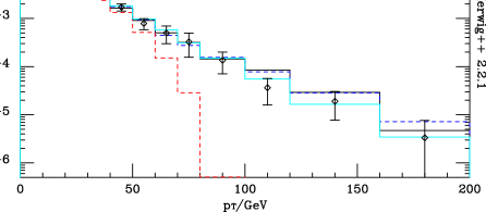
ERWIG++
For validation purposes, Fig. 5.3 presents a comparison of the boson transverse momentum distribution, (assuming no ) between Tevatron data (taken from Ref. [124]) and the three possible methods: leading order, MC@NLO and POWHEG. The plots include events in the invariant mass range . The MC@NLO and POWHEG distributions are in agreement with the data within the statistical Monte Carlo and experimental uncertainties. The leading-order distribution is cut off at the mass since this provides the only relevant scale in the parton shower, whereas the MC@NLO and POWHEG distributions extend to higher transverse momentum. The different factorisation schemes given, DIS and , arise due to the arbitrariness of the prescription in how the finite contributions to the PDFs are treated when factorising the logarithmic singularities. The subsequent figures in this section represent simulations made for the LHC running at 14 TeV proton-proton centre-of-mass energy.
Figure 5.4 shows the variation of the NLO cross section for a 1 TeV left-handed in the invariant mass range GeV with factorisation scale, , for a fixed renormalisation scale using the scheme. The LO variation with PDF scale is also shown in an equivalent range. The values have been normalised to the cross sections at the default scales (default NLO) and (default LO). In the NLO case the renormalisation scale was held fixed at . The NLO cross section calculation appears to be slightly more stable than the LO calculation. The -factor at was found to be and the LO cross section at was found to be pb.

Figures 5.5 and 5.6 show the transverse mass distributions (in this case we show a ‘theoretical’ transverse mass, defined by ) at LO and NLO for a at masses and widths of and , for purely left-handed () and purely right-handed () couplings to fermions respectively. Figures 5.7 and 5.8 show the corresponding transverse momentum distributions. In this case the LO distribution cuts off at the mass. The effect is less visible for higher masses. Figure 5.9 shows a comparison between the different methods of the rapidity, longitudinal momentum and mass distributions for a right-handed of mass and width at the LHC.
Finally, Fig. 5.10 shows a comparison between the left- and right-handed ‘experimental’ transverse mass distributions at NLO (defined by , using the missing transverse energy and momentum, and the lepton transverse energy and momentum), using the MC@NLO method. The importance of the interference between the SM and the can be clearly observed: the differential cross section in the region below in the purely left-handed () case is reduced in comparison to the purely right-handed () case. For a transverse mass greater than the on-shell mass of the , the interference term becomes positive for the left-handed case, although this effect is not significant. The SM contribution, in the absence of a boson, is given for comparison in both figures. In the right-handed case the contribution of the is simply additive to the SM contribution.
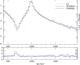
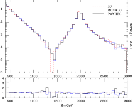
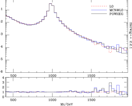
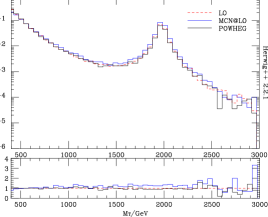
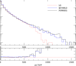
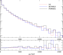
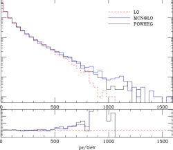
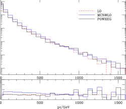
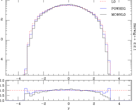
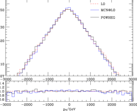
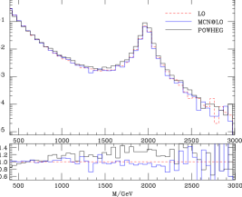
5.2.7 Extraction of limits
In appendix E.1 we provide a general method for discriminating between two models given a set of events. Here we apply this method to extract observation limits on the mass and width at LO. A stand-alone program was written to calculate the quantity at matrix element level, given by Eq. (E.5):
The ‘true’ underlying theory, labelled T, was assumed to contain a at a predefined mass and theory S was taken to be the SM. Some comments are appropriate:
-
•
Although the total width was being varied, the decay width to fermions was always assumed to be .
-
•
In a real experiment the mass would be unknown and maximum likelihood methods should be used to fit the parameters if significant deviation from the SM is found.
-
•
The parameter can become very large if a small number of unlikely events occur, which favour one theory over the other. Experimentally this is unrealistic since ‘unlikely’ events could be the effect of background or detector effects. To take these into account, one has to introduce nuisance parameters whose behaviour, at this level of analysis, have to be chosen arbitrarily. Here we avoid the introduction of such arbitrary parameters.
-
•
The detection curves were drawn for specific data distributions and fluctuations are expected. In other words, the plots correspond to a specific ‘experimental’ data set.
-
•
The ratio of the prior probability distributions, , was taken to be equal to unity throughout this analysis: i.e. we assume both models are equally likely prior to the ‘experiment’.
-
•
A rapidity cut on the leptons corresponding to for the LHC and for the Tevatron was applied to take into account the acceptance regions of the detectors.
-
•
The distributions and were calculated using the Monte Carlo event generator itself at higher statistics () than the required number of events to reduce the required computer time. The sum over in Eq. (E.5) was taken over the bins of these distributions and not individual events.
The limits were drawn on a width-mass plane as detection curves, where is a constant. The variable can be interpreted as a probability ratio and a discovery curve can be interpreted as the limit where the existence of a is discovered with certainty . For example if , then the detection curve represents the confidence level. The LO detection curves can be seen, for different integrated luminosities at the LHC (14 TeV), in Fig 5.11 for a right-handed and Fig. 5.12 for a left-handed . The curves correspond to a single data sample at each point, and therefore there are large statistical fluctuations, particularly in the low-luminosity curves. A comparison between the curves for a left- and right-handed is shown in Fig. 5.13. It can be observed that a left-handed has a slightly higher detection reach, especially at larger widths. By examining Figs. 5.11 and 5.12, we deduce that the maximum detection reach at the LHC, for example using an integrated luminosity of 100 fb-1, for a decaying primarily to fermions (), is .
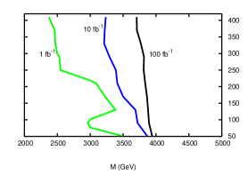
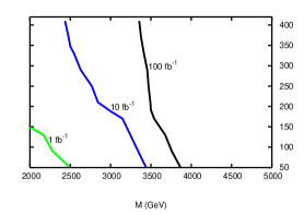
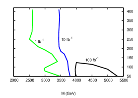
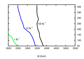
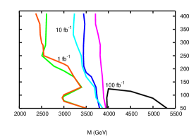
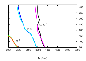
We also show the expected limit at the Tevatron (1.96 TeV) in Fig. 5.14 with an integrated luminosity of 2 fb-1, both at leading and next-to-leading (see below) orders. When the is only allowed to decay to fermions, i.e. has width , the predicted detection limit for is . This is expected to be reduced by experimental effects. Since the available centre-of-mass energy at the Tevatron is , we expect the saturation of the detection reach to come at about without interference and slightly higher in the left-handed case when interference effects are included. The Tevatron NLO case does not exhibit any substantial difference from the LO case.
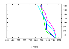
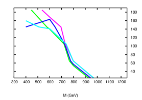
We have performed an equivalent analysis using the NLO method POWHEG at matrix element level to improve computational time. Working at matrix element level with the POWHEG method is justified since the transverse mass distribution is not significantly altered after shower and hadronization and no difficulties arise due to negatively-weighted events, as would be the case in the MC@NLO case. The comments given at the beginning of the section for the LO analysis also apply to the NLO analysis. The results are shown in Figs. 5.15 and 5.16 in comparison to the LO results. In the right-handed chirality scenario, NLO implies a lower detection reach than indicated at LO. The situation is more complicated in the left-handed case where the NLO case implies a slightly higher reach for larger widths.
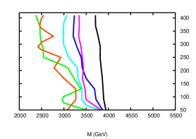
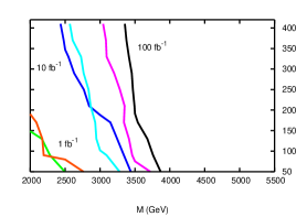
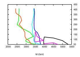
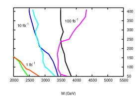
To investigate the dependence of the NLO results on the factorisation scale we have reproduced the contours for the right-handed LHC case with an integrated luminosity of 10 fb-1 at different values of while keeping the renormalisation scale fixed, using the scheme. The results are shown in Fig. 5.17. The curves show that the factorisation scale does not affect the detection reach substantially, for example only shifting the contour at a width of from to going from to .
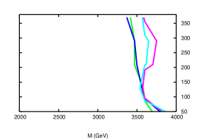
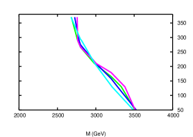
5.2.8 Conclusions
We have presented a Monte Carlo implementation of the Drell-Yan production of new charged heavy vector bosons. We have considered the interference effects with the Standard Model boson, allowing arbitrary chiral couplings to the leptons and quarks. Moreover, the implementation is correct up to next-to-leading order in QCD, via the MC@NLO and POWHEG methods using the H ERWIG++ event generator. We have presented a sample of results at both leading and next-to-leading orders. As expected, the LO and NLO boson transverse momentum distributions were found to differ significantly, the NLO extending to higher . The dilepton transverse mass, invariant mass, rapidity and -momentum distributions were found not to be significantly altered by the NLO treatment. The total cross section was found to increase in the NLO case by a factor of in the region of interest.
Subsequently we applied a theoretical discrimination method to the reference model to obtain mass-width observation curves for left- and right-handed chiralities of the both at LO and NLO (POWHEG). The NLO curves were shown not to vary significantly with factorisation scale. The event generator used throughout this analysis, Wpnlo, is fully customisable and publicly available [107].
5.3 Searching for third-generation composite leptoquarks
5.3.1 Introduction
The riddle of electroweak symmetry breaking (EWSB), and specifically the hierarchy problem we have described in section 2.3.1.1, can be addressed in natural way via the introduction of new physics in the form of a new strong force. An example of new strong dynamics is ‘technicolour’ - a theory in which EWSB can be explained without adding any fundamental scalars and the Higgs boson arises as a composite particle of some new fermion states. This solution is natural in a literal sense, meaning that we have already observed an example present in Nature: the hierarchy between the Planck scale () and the proton mass () is a result of the logarithmic running of the QCD coupling constant and the onset of the strong coupling in the infrared.
The Higgs mechanism must explain not only how the masses of the gauge bosons arise, but also the origin of the fermion masses. We have already described the conventional mechanism of fermion mass generation in the SM in section 2.2.2.2. This is done conventionally via the so-called ‘Yukawa’ interaction. Before EWSB we have, e.g. for the fermions of the third generation, couplings of the form:
| (5.24) |
where is the top quark Yukawa coupling, is the third generation fermion doublet, is the fundamental scalar Higgs operator and is the third generation fermion singlet. In theories of strong dynamics EWSB it is usual to assume that masses arise via a similar Yukawa-type interaction:
| (5.25) |
where we have included a suppression scale , the scale at which the flavour physics arises, is the mass dimension of the scalar Higgs operator, now taken to be and is a ‘strong’ Yukawa coupling (which is dimensionless like ). However, in the framework of an effective theory, other terms will necessarily need to be added to the full Lagrangian. One of these terms has the form:
| (5.26) |
This four-fermion operator is potentially catastrophic since it can induce flavour-changing neutral currents (FCNCs) that can contribute to meson mixing. For example, an operator involving two strange quarks and two down quarks, of the form , would contribute to mixing. This type of FCNCs have been well-measured experimentally and to satisfy the existing constraints, one needs to choose the suppression scale to be . In the SM we can set as large as we wish and the FCNCs decouple from the theory since the SM Yukawa interaction term of Eq. (5.24) is not suppressed by any power of . In theories of strong dynamics, in general and hence we cannot set the scale to be arbitrarily high, otherwise there is a risk of decoupling the Yukawa term of Eq. (5.25) as well, rendering the theory incapable of producing fermion masses naturally. This is particularly true for the large top quark mass.
A solution to this issue, that was proposed long ago [125], introduces composite fermions which arise due to the strong dynamics. The elementary fermions do not couple directly to the scalar Higgs operator; instead they mix with the composite fermions via bilinear interactions. Schematically, the Lagrangian terms relevant to the generation of mass for the third generation is given by
| (5.27) |
where and are the strong coupling mass scale and coupling respectively, and are the mixing parameters of the theory, corresponding to the left- and right-handed top quark multiplets, and are composite left- and right-handed fermions respectively, and is the composite scalar Higgs operator. Note that there are two mixing parameters for each fermion, one for each chirality. As an example, the fermions could be technibaryons, composites of some new ‘technifermions’ in a technicolour theory, just as the protons are composites of quarks in QCD. The Lagrangian produces an effective Yukawa term for the elementary fermions. By examining Fig. 5.18:
| (5.28) |
where we have used the mixing parameters to define the top Yukawa coupling:
| (5.29) |
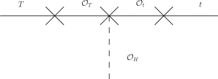
The mechanism is not only capable of producing fermion masses, but also offers the hope that the observed hierarchies of masses and mixings of the SM fermions may be related to the electroweak hierarchy via strong-coupling effects. This is because the third generation can be considered to be the ‘most composite’ and hence should have masses closest to the strong dynamics scale [125].
It is obvious now that the new strong sector must know about colour and must contain, at the very least, colour-triplet fermionic resonances that mix with the elementary colour-triplets and make the observed fermions. It is reasonable to also expect the strong sector to contain other coloured resonances. It may contain bosonic resonances that, depending on their gauge charges, may be able to couple to a lepton and a quark, playing the role of the leptoquark states. For example, in Ref. [125], in which the fermionic resonances were the technibaryons of , the model would also contain technimesons that would be able to act as leptoquarks.
It is easy to make an estimate of the magnitude of the leptoquark couplings to fermions in such models. These arise in much the same way as the effective Higgs boson couplings, through the following schematic Lagrangian:
| (5.30) |
where is one of the quark mixing parameters, is one of the lepton mixing parameters and is a leptoquark operator with the correct gauge charges to couple to a composite quark and a composite lepton. It is important to note that the mixing parameters that appear in Eq. (5.30) are the same as those that appear in (Eq. (5.27)). The leptoquark effective coupling can then be calculated by considering the schematic diagram in Fig. 5.19. We can deduce that the form of the coupling is
| (5.31) |
where we have defined the leptoquark coupling to quarks and leptons, . We can make estimates of the magnitude of the coupling using the measured Yukawa couplings if we restrict the mixing parameters to be equal for the quarks and leptons of each generation:
| (5.32) |
where and (left-handed doublets), (right-handed up-type singlets), (right-handed down-type singlets), (hypothetical right-handed neutrinos) and . We can then use the measured Yukawa couplings and estimate each of the mixing parameters that appear in Eq. (5.29) for the quarks and leptons:
| (5.33) |
We can substitute these estimates into the leptoquark coupling to fermions defined in Eq. (5.31), to obtain an estimate in terms of the measured Yukawa couplings:
| (5.34) |
From the above equation it is easy to see that couplings to quarks of the third generation will dominate in this type of models. The SM fermion Yukawa couplings (taken from Ref. [126]) are given in Table 5.1 and the resulting estimates of the leptoquark couplings are given in Table 5.2. These estimates evade the constraints coming from flavour experiments, for leptoquark masses even down to , which may arise if the leptoquarks appear as pseudo-Nambu-Goldstone bosons [126].
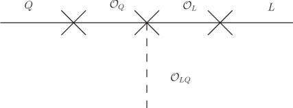
| Fermion | Yukawa, |
|---|---|
| Lepton Quark | 1 | 2 | 3 |
|---|---|---|---|
| 1 | |||
| 2 | |||
| 3 |
Since the leptoquark couplings to light fermions are highly suppressed, the only relevant couplings for direct collider production and detection are those to third-generation fermions.777For an alternative scenario with leptoquarks of this type, see [127]. As a result, the leptoquark states will decay exclusively to third-generation fermions, that is to or or or . Naïvely, since the leptoquark couplings scale roughly with the Yukawa couplings, and since the bounds preclude a leptoquark mass below ,888Searches at D0 for third-generation scalar leptoquarks decaying exclusively to or yield bounds of 210 GeV [128] and 229 GeV [129] respectively. one might conclude that decays involving the top must dominate. However, we shall see later that the gauge quantum numbers sometimes preclude couplings to top quarks and, of course, unknown global symmetries may also preclude one or more couplings. Thus we consider all four possible couplings.
Since leptoquarks couple dominantly to third-generation quarks and leptons, pair-production through colour gauge interactions will overwhelmingly dominate single-production at the LHC. The channels of interest therefore involve pair-wise combinations of or or or .999Note that third-generation lepton-quark couplings are also possible in -parity-violating supersymmetric theories. The and channels already have been the subject of searches at the Tevatron [129, 128], and can be adapted easily for the LHC. The use of novel kinematic variables such as in this channel may well improve the prospects for discovery and mass measurement. The two channels involving the top require more ingenuity, but merit investigation.
In the present section we perform the first detailed phenomenological study of the possible production of such states at the LHC. In section 5.3.2 we briefly review their quantum numbers, couplings and decay modes, which we have implemented in the H ERWIG++ event generator.101010P YTHIA [130, 45, 131] contains an implementation of a single scalar leptoquark of arbitrary flavour. This allows us to propose and investigate strategies for reconstructing third-generation leptoquark masses from their decay products, including those that involve top quarks, in the following sections. Our conclusions are presented in section 5.3.9.
Although we focus here on direct searches at the LHC, there are also promising channels for indirect searches, namely in and at LHCb, in and , in conversion in nuclei, and in at future B factories [126].
5.3.2 Phenomenology
5.3.2.1 Scalar leptoquark pair-production
We focus on scalar leptoquarks in the present study since their bosonic couplings are determined completely by QCD and hence their production cross sections only depend on their masses. Moreover, the lightest (and most easily accessible) leptoquarks in these scenarios arise as scalar pseudo-Nambu-Goldstone bosons. The type of leptoquarks we are considering are predominantly pair-produced via gluon-gluon fusion or quark-anti-quark annihilation, due to the fact that they couple to the third-generation quarks and leptons. Only charge-conjugate leptoquarks can be produced in this way: associated production of different leptoquarks is forbidden since it would not conserve the Standard Model gauge quantum numbers. Single-production in association with a lepton is allowed but at a LHC it becomes dominant at leptoquark masses of about , at which point the total cross section, , is already too low for discovery.
5.3.2.2 Effective Lagrangian for interactions with gluons
The effective Lagrangian describing the interaction of the scalar leptoquarks with gluons is [132]
| (5.35) |
where is a scalar leptoquark, are colour indices, the field strength tensor of the gluon field is given by
| (5.36) |
and the covariant derivative is
| (5.37) |
The Feynman rules that result from this Lagrangian and the diagrams that contribute to pair-production of scalar leptoquarks are given in appendix F.1. Expressions for the cross sections are given in appendix B.
5.3.2.3 Non-derivative fermion couplings
The effective Lagrangian that describes the possible non-derivative couplings of the scalar leptoquarks to third-generation quarks and leptons is given by [133]
| (5.38) | |||||
where the are the Pauli matrices, and are quark and lepton doublets respectively and , and are the corresponding singlet fields. We denote charge-conjugate fields by , where the superscript c implies charge conjugation. In Table 5.3 we give the quantum numbers for the five types of non-derivatively coupled scalar leptoquarks: the -singlet complex scalars and , the -triplet complex scalar and the -doublets and .
| Name | Decay mode | H
ERWIG++ |
||||
| 0 | 1/3 | 1/3 | , , | -9911561 | ||
| 0 | 4/3 | 4/3 | -9921551 | |||
| +1 | 1/3 | 4/3 | -9931551 | |||
| 0 | 1/3 | 1/3 | , | -9931561 | ||
| -1 | 1/3 | -2/3 | -9931661 | |||
| +1/2 | 7/6 | 5/3 | 9941561 | |||
| -1/2 | 7/6 | 2/3 | , | 9941551 | ||
| +1/2 | 1/6 | 2/3 | 9951551 | |||
| -1/2 | 1/6 | -1/3 | 9951651 |
The numbering scheme used in our implementation of scalar leptoquarks in H ERWIG++ is also given in Table 5.3. The particles are numbered as , where distinguishes the representation of the standard model gauge group, is the lowest possible number chosen to relate the leptoquark to the Particle Data Group (PDG) codes of decaying fermions, and , where is the particle spin. The sign of the PDG code is negative for colour anti-triplets and positive for colour triplets. Hence, is the ‘first’ type of leptoquark, , and can decay to particles with codes () and ().
Notice that the first three kinds of leptoquarks, the , and the triplet are colour anti-triplets and the particles (as opposed to the anti-particles) decay into an anti-lepton and an anti-quark. This is contrast to the and doublets, which are colour-triplets and decay into quarks and anti-leptons.
5.3.2.4 Derivative fermion couplings
We also consider leptoquarks that couple derivatively to the quarks and leptons. The couplings of the leptoquarks to fermions involve three fields, and hence two independent positions for the derivative to act, modulo integration by parts. Here, we choose to place the derivative on either the quark or the lepton, such that the Lagrangian is given by
where the index and , , denotes the momentum of the lepton or quark.
| Name | Decay mode | H
ERWIG++ |
||||
| 0 | 2/3 | 2/3 | 9961551 | |||
| 0 | 5/3 | 5/3 | 9971561 | |||
| +1 | 2/3 | 5/3 | 9981561 | |||
| 0 | 2/3 | 2/3 | 9981551 | |||
| -1 | 2/3 | -1/3 | 9981651 | |||
| +1/2 | 5/6 | 4/3 | -9991551 | |||
| -1/2 | 5/6 | 1/3 | -9991561 | |||
| +1/2 | -1/6 | 1/3 | -9901561 | |||
| -1/2 | -1/6 | -2/3 | -9901661 |
The charges of the primed scalar states appear in Table 5.4; they correspond, of course, to those of vector leptoquarks. Notice that whereas the is a colour anti-triplet, is a colour triplet and so on.
Consider a leptoquark that couples derivatively to fermions in the following way:
| (5.40) |
where the is the sigma model scale for the strong dynamics. Consider the decay of the to on-shell fermions via the coupling . We then have
| (5.41) | |||||
Note that the chirality of one decay product is reversed in each term by the mass insertion, which breaks the gauge symmetry. An equivalent manipulation is given in appendix F.2 for terms that contain conjugate fields. For simplicity, we choose to set the quark and lepton primed couplings for each term equal, , where represents , or . As a result of the above manipulation, an effective Lagrangian for the on-shell decay of a scalar leptoquark may be written as
| (5.42) | |||||
| (5.43) | |||||
converting all the derivative couplings to ones that look like those for the unprimed leptoquarks, with the lepton or fermion masses appearing in the coupling. See appendix F.2 for the full effective Lagrangian. Since the scale is typically a few hundred GeV, couplings proportional to the top quark mass are expected to dominate when the corresponding decays are kinematically allowed. The on-shell fermion assumption is realistic since the widths of the fermions are small in comparison to their masses and hence off-shell effects are negligible.
5.3.2.5 Decay widths
The decay width of non-derivatively coupled scalar leptoquarks in the limit of massless quarks and leptons is given by [133]
| (5.44) |
where the couplings for the types of leptoquarks we are considering are given in Table 5.5 in terms of the couplings that appear in the Lagrangian. The couplings are taken to be real. The expression gives, for quark-lepton couplings and leptoquark mass of , a width of .
| Name | |||
| 0 | 0 | ||
| 0 | 0 | ||
| 0 | |||
| 0 | 0 | ||
| 0 | |||
| 0 | |||
| 0 | 0 | ||
| 0 | 0 |
The decay width to massive is further suppressed by a phase-space factor compared to the massless quark and lepton width [129]:
| (5.45) |
where are the squared ratios respectively.
| Name | |||
| 0 | |||
| 0 | |||
| 0 | 0 | ||
| 0 | |||
| 0 | |||
| 0 | 0 |
| Decay mode | Decay width (GeV) | BR |
|---|---|---|
| 0.1040 | 0.5666 | |
| 0.07956 | 0.4334 | |
| 0.07956 | 1 | |
| 0.1591 | 1 | |
| 0.05225 | 0.3964 | |
| 0.07956 | 0.6036 | |
| 0.1045 | 1 | |
| 0.1040 | 1 | |
| 0.07956 | 0.6036 | |
| 0.05225 | 0.3964 | |
| 0.07956 | 1 | |
| 0.07956 | 1 |
Table 5.6 shows the couplings for the primed, derivatively-coupled, scalar leptoquarks. The expression for the width given in Eq. (5.44) remains unchanged in the case of the primed leptoquarks, with the couplings taking the appropriate values. Tables 5.7 and 5.8 show example decay widths and branching ratios for scalar leptoquarks of mass and couplings . In the case of derivatively coupled leptoquarks we choose a suppression scale .
| Decay mode | Decay width (GeV) | BR |
| 0.0036 | ||
| 0.001239 | 0.9964 | |
| 0.001239 | 1 | |
| 0.002478 | 1 | |
| 0.0010 | ||
| 0.001239 | 0.9990 | |
| 1 | ||
| 1 | ||
| 0.001239 | 0.9991 | |
| 0.0009 | ||
| 0.001234 | 1 | |
| 0.001239 | 1 |
5.3.3 Reconstruction strategies
Table 5.9 provides an overview of our suggested reconstruction strategies for the different types of leptoquarks. The ‘stransverse’ mass variable, , which appears in the table has been defined previously in Ref. [134], for the case of identical semi-invisible pair decays as
| (5.46) |
where the minimisation is taken over and , the transverse momenta of the invisible particles, with the constraint that their sum equals , the total missing transverse momentum, and and are the transverse masses calculated for the two decay chains. We assume that the invisible particles are massless and use the jet masses in our definitions of . The new variables and will be defined in section 5.3.6.1.
We present our analysis of the mass reconstruction techniques for each pair-production decay mode separately, initially at parton level and then at detector level, including discussion of the relevant backgrounds. We focus on the singlet, triplet and doublet and outline how to generalise the strategy to all the leptoquark multiplets.
It is evident from Tables 5.7 and 5.8 that the leptoquark decay widths are generally much smaller than the resolution of the detector components, and hence our analysis is not sensitive to the decay widths. Throughout the following we have set the leptoquark couplings to fermions to the value . This value is close to the estimate of the leptoquark coupling to third-generation quarks and leptons () derived using the measured fermion Yukawa couplings and the assumptions given towards the end of Section 5.3.1 (see Tables 5.1 and 5.2). The resulting width-to-mass ratio for the leptoquarks corresponding to this coupling, according to Eq. (5.44), is .
We use the H ERWIG++ event generator to generate a number of events corresponding to an integrated luminosity of fb-1 of the relevant signal and background samples. Subsequently we use the Delphes framework [135] to simulate the detector effects and assess the feasibility of reconstruction in an experimental situation.111111Delphes is a framework for fast simulation of a general-purpose collider experiment. Delphes includes the most crucial experimental features: the geometry of the central detector, the effect of the magnetic field on the tracks, reconstruction of photons, leptons, -jets, -jets and missing transverse energy. It contains simplifications such as idealised geometry, no cracks and no dead material. We use the default parameter settings in the Delphes package that correspond to the ATLAS detector. Crucial features of our analysis are both - and -tagging of jets and we caution the reader to take into consideration that the relevant efficiencies will contain a degree of uncertainty at the early stages of the LHC experiment. The -tagging present in the Delphes framework assumes an efficiency of 40% if the jet has a parent -quark, 10% if the jet has a parent -quark and 1% if the jet is light (i.e. originating from , , or ). The identification of hadronic -jets is consistent with the one applied in a full detector simulation. The resulting efficiencies for hadronic -jets are in satisfactory agreement with those assumed by ATLAS and CMS. See [135] for further details.
Throughout the analysis we apply transverse momentum cuts of at least . Since we are always working with high-transverse momentum objects, we can assume that pile-up arising due to secondary proton-proton collisions is under experimental control. See, for example, the ATLAS study in Ref. [77].
| modes | types | technique |
|---|---|---|
| , | , mass constraints | |
| edge reconstruction (, , ) | ||
| , , | two , mass constraints | |
| , | full reconstruction | |
| , , | ||
| , | ||
| , | two , mass constraints | |
| , , | full reconstruction | |
| , | ||
| , , | ||
| , | , mass constraints | |
| edge reconstruction (, , ) |
5.3.4 decay mode
We examine the possibility of full reconstruction of the topology shown in Fig. 5.20, where we have, for example, and , where and represent one or more neutrinos coming from the decays and can be either a muon or an electron. We can assume that the neutrinos associated with the decays of the s are collinear with the direction of the jets associated with them. The validity of this assumption has been confirmed using H ERWIG++ , for leptoquarks of masses 1, 0.4 and 0.25 TeV, as may be seen in Fig. 5.21, which shows the distribution of between the momenta of the jet partons and the invisibles. The assumption is employed in our reconstruction of any leptoquark decay mode containing a -jet.
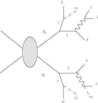

The top quark branching ratios are for the semi-leptonic modes and for the hadronic top modes. These appear twice since we have either the or , resulting in an overall factor for the top decay modes. The branching ratios and cross sections for production depend on the leptoquark mass and coupling and are shown in Table 5.10, where the last column is the resulting cross section for the topology under study. We focus on leptoquarks since these are clearly not excluded by direct searches at present and still provide a sufficient number of events to be potentially discovered at a reasonable luminosity (10 fb-1) at TeV.
| (GeV) | (pb) | BR() | (pb) |
| 174.2 (= ) | 141(1) | 0. | 0. |
| 250 | 24.3(3) | 0.34 | 0.729 |
| 400 | 2.000(7) | 0.567 | 0.188 |
| 500 | 0.561(6) | 0.606 | 0.06 |
| 1000 | 5.94(7) | 0.65 | |
| (GeV) | (pb) | - | (pb) |
| 174.2 | 834(1) | - | 242 |
5.3.4.1 Kinematic reconstruction
The final states of processes contain many decay products including neutrinos. If the system has a large enough number of kinematical constraints, such as mass-shell conditions and the balance of the total transverse momentum, we can completely reconstruct the kinematics of the system. The numbers of unknown variables and constraints are summarised in Table 5.11 for each decay pattern of the tops: (1) both tops decay hadronically, (2) one top decays semi-leptonically and another hadronically and (3) both tops decay semi-leptonically.
| Decay type | # of unknowns | # of constraints |
|---|---|---|
| (1) had,had | ||
| (2) had,lep | ||
| (3) lep,lep |
As mentioned above, we assume -neutrinos are collinear to the -jets, leaving two unknown parameters associated with the taus, namely the energy ratios (, ) which are defined (neglecting masses) by
| (5.47) |
where , and are the four-momenta of the leptons, -jets and -neutrinos, respectively. Under this assumption, the unknown variables in Table 5.11 are the mass of the leptoquark, the 4-momenta of neutrinos from leptonic top decays and the energy fractions associated with the neutrinos from the tau decays. The mass-shell conditions that could constrain the unknown variables are counted in Table 5.11, i.e. the mass-shell conditions on , leptonic top, and from leptonic top decay.
It is only possible to wholly reconstruct the kinematics of a single event in decay types (1) and (2). In decays of type (1), it would be difficult to reconstruct both hadronic tops because of the large combinatorial background. Thus, we focus on decay type (2) and attempt to determine the leptoquark mass. As we show in appendix F.3, in this case one obtains a quartic equation for the energy ratio , and hence in general up to four solutions for the leptoquark mass, at least one of which should be close to the true value if the visible momenta and missing transverse momenta are well-measured.
5.3.4.2 Parton-level reconstruction
We first perform the analysis of the hard process (no initial- or final-state radiation, no underlying event) at parton level without considering experimental or combinatoric effects, to examine its feasibility. For the majority of cases there are only two physical, approximately degenerate, solutions, which are close to the true leptoquark mass. The numerical solution of the quartic equation sometimes fails to yield real roots. The results for true leptoquark masses TeV are shown in Fig. 5.22, which includes histograms of the solutions obtained for events. The histogram includes a bin at 0 where the events without real solution are placed. These amount to about 10% of the total events. At this level the reconstruction technique provides a good estimate of the leptoquark mass for all the trial true masses, lying within a few GeV of the true mass.


5.3.4.3 Experimental reconstruction
We consider an leptoquark with mass , for which the cross section for production and decay into the topology of Fig. 5.20, , is pb. The most significant background in this scenario is production, with two extra jets misidentified as s and subsequent decay of the tops into . The cross section for this process is pb, overwhelming to begin with. There is also potentially an irreducible background which, for a Higgs boson of mass , has a cross section of approximately 65 fb. Since one of the main rejection mechanisms is the reconstruction through the solution of the kinematic equations, we do not expect this background to contribute significantly in the signal region.
We simulate the events with QCD initial-state radiation (ISR), final-state radiation (FSR) and underlying event (UE). We use the default jet algorithm provided by the Delphes package for the ATLAS configuration, the anti- with the parameter set to . We then demand a set of relatively loose cuts on the full and samples, since in a real experiment we would not be able to separate the different decay modes of the top quark or leptoquark. The cuts applied are the following:
-
•
The existence of a lepton in the event, being either a muon or electron, with .
-
•
A minimum of 6 jets.
-
•
The missing transverse momentum in the event, .
-
•
Two -tagged jets, with the extra requirement that they both have .
-
•
No jets tagged as both - and -jets simultaneously.
We also require that the highest- lepton is at a distance from the -tagged jets, since electrons may create a candidate in the jet collection as well as the lepton collection. The analysis then breaks up into different branches according to the number of -tagged jets in an event:
-
•
Two -tagged jets: we look for one or two further jets (with ) that form an invariant mass close to the top mass, within . One -jet is then associated with the semi-leptonic top decay and the other with the hadronic top decay.
-
•
One or no -tagged jets: when there is one -tagged jet, we check whether it will satisfy the top mass conditions with any other (one or two) remaining jets, otherwise we associate it with the semi-leptonic top. If so, we look for any two or three jets that satisfy the top mass conditions, and form the hadronic top within a mass window. For the remaining -jets (or if there are no -jets) we look for the remaining highest- jets. Any jets that are found in this way and called -jets are required to have a .
No solutions are found in the sample of 70 signal events passing the cuts, if we require the ratios to be purely real. Hence, the solutions to the quartic equation for the momentum ratios , described in appendix F.3, are now allowed to be complex in order to provide some signal. This is valid since even true leptoquark events are smeared and distorted by detector and QCD effects. We use the real part of as an input to the calculation of the rest of the kinematic variables. This is reasonable since the experimental effects are expected to ‘smear’ the position of the true value of in all directions in the complex plane. The effect is shown in Fig. 5.23, where we plot the real and imaginary parts of for the events that have passed the kinematic cuts. Evidently, there is a concentration of solutions around the positive real axis, an effect exemplified by Fig. 5.24, where we show the ratio of the real part of and its modulus. We have further demanded that the resulting momentum fractions are physical: , resulting in only real solutions for . Figure 5.25 shows a reconstruction plot for leptoquarks of mass . Note that each event was given weight 1, distributed evenly amongst the solutions it yields. In the case of complex , we assume there is one solution corresponding to the complex conjugate pair.
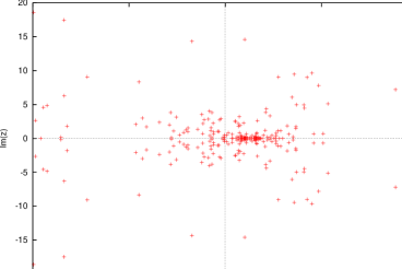


Although the cuts applied are relatively weak, most of the background rejection comes from the requirement of two -tagged jets. The background does not produce solutions in the physical region often enough to be significant.
5.3.5 decay modes
We can obtain the mass of the leptoquarks when both of them decay into or using the variable (Eq. (5.46)). Examples of these decay mode are and .
5.3.5.1 Parton-level reconstruction
At parton level, the and decay modes are similar and hence we consider only the latter here. We first construct the variable using the parton-level -quark 4-momenta, in the absence of any experimental effects, ISR, FSR or UE. The result is shown in Fig. 5.26 for TeV, confirming the expected sharp edge in these idealised conditions.

5.3.5.2 Experimental reconstruction
As before, we use the Delphes framework to simulate the detector effects, with the settings stated in section 5.3.3. We demand two -tagged jets in both the and cases. In the latter we search for combinations of 1 or 2 jets with the -tagged jets which form the top mass within a window of . We require the following cuts for the case, on the full sample:
-
•
Two -tagged jets with each.
-
•
No electrons or muons in the event.
-
•
Missing transverse energy .
For the case we require the following cuts on the sample:
-
•
Two -tagged jets with each.
-
•
No electrons or muons in the event.
-
•
Missing transverse energy .
The resulting distributions for the signal (blue) and background (red) can be seen in Fig. 5.27.


The mode appears to be more challenging to reconstruct than the mode. This is due to the fact that the background is very similar to the signal and the difficulties that are present in reconstructing hadronic tops. Nevertheless, as the results show, it may be possible to observe an excess over the distribution of the background and provide an estimate of the mass.
5.3.6 decay modes
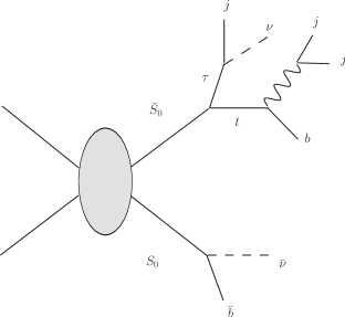
One possible event topology for the processes is shown in Fig. 5.28. When the top decays hadronically the system has two neutrinos, one from an decay and another from a decay. If we can reconstruct the hadronic top correctly, we can simply use to obtain the mass of the leptoquarks. Similar topology is present in the decay mode.
It is known that the information from is the same as that from the ‘minimal kinetic constraints’, in events where two identical particles decay to missing particles with the same mass [136, 137, 138]. As discussed in section 5.3.4, in this type of event, we can take advantage of the fact that, to a good approximation, the neutrino from a decay is travelling almost collinearly to the -jet in the lab frame. By including this constraint, we can define kinematical variables, and , which perform better than at parton level, as we will show in the following subsections.
5.3.6.1 Kinematic reconstruction
In the collinearity approximation, neglecting masses, we can write
| (5.48) |
The second neutrino comes directly from the decay associated with a -jet. The transverse components of the momentum of this neutrino are constrained by
| (5.49) |
There are two unknown parameters left, and . In terms of these, we define two invariant mass variables:
| (5.50) |
and
Note that does not depend on and is a monotonically increasing function of because . We can now define two -like variables:
| (5.52) |
and
| (5.53) |
where minimisation is taken for all possible (, ). By construction, both these quantities have an upper bound equal to the leptoquark mass:
| (5.54) |
Furthermore, we show in appendix F.4 that
| (5.55) |
5.3.6.2 Parton-level reconstruction


Figure 5.29 shows the parton-level distributions of , and for 1000 events. We took only the true combination of the jet assignment. As can be seen, all the distributions have clear edge structures at the input leptoquark mass of 400 GeV.
In order to compare these variables we took their differences, shown in Fig. 5.30. The relation is seen to hold on an event-by-event basis. This implies that and are more powerful than for determining the mass of the leptoquark, at least at parton level.


5.3.6.3 Experimental reconstruction
The settings for experimental reconstruction used for the Delphes fast simulation remain unaltered in this analysis (see section 5.3.3). We apply the following event selection cuts to the full signal and the background:
-
•
At least four jets found in each event.
-
•
Exactly one -tagged jet with .
-
•
No, one or two -tagged jets with .
-
•
Missing transverse energy, .
For the -jet originating from the leptoquark decay, we choose the highest- -tagged jet when there are two -tagged jets and the highest- jet (excluding the -tagged jet) when there are no -tagged jets. We use all the remaining jets with , (not identified as the -jet from the leptoquark) to search for one, two or three jets that form an invariant mass close to the top mass, within a window. We apply the additional constraint that the difference between the of the -tagged jet and the of the -tagged jet, . This eliminates a high fraction of the background since the s in that sample originate from the decay and are expected to have lower on average than the s that originate directly from the top. On the contrary, in the leptoquark signal the and transverse momenta are expected to be of the same magnitude on average.
The resulting distributions are shown in Fig. 5.31. Due to the low number of events passing the selection cuts, it is not obvious whether the observable performs better than and . However, we checked that the three distributions satisfy the same inequalities presented in Fig. 5.30 for the parton-level reconstruction.


The reconstruction strategy for the mode follows the technique described in section 5.3.6.1 for the case, with the simple replacement . The assignment of -jets and top-jets is performed in the same way as in the analysis, with the following cuts applied to the full sample:
-
•
At least four jets found in each event.
-
•
Exactly one -tagged jet with .
-
•
No, one or two -tagged jets with .
-
•
Missing transverse energy, .
There is also a cut on the reconstructed hadronic top jet, of and that its invariant mass lies within of the top mass. The results are shown in Fig. 5.32. Note that the background that would be present due to the leptoquark has not been included.
Although at parton level, the variable performs better than and , it seems to become unstable after including experimental effects, with some events failing to produce a value within the range of the plots shown in Fig. 5.32. The origin of the instability is the additional assumption of the leptoquark masses being equal, which is satisfied at parton level (up to small width effects) but does not hold exactly after detector simulation. For the events for which no solution is found, we assign . Even after this readjustment, there are a few events for which a solution for is found and lies outside the region shown. Therefore, and appear to be preferable as experimental observables.


5.3.7 decay mode
5.3.7.1 Kinematic reconstruction
The mode can be fully reconstructed if one again assumes collinearity of the -jets and -neutrinos: (, ). This implies that the missing momentum from each can be written as . Hence, we may write the following equalities for the components of the measured missing transverse momentum:
| (5.56) |
The above equations may be written in matrix form and inverted to give
| (5.57) |
Now the invariant mass of each of the two leptoquarks may be written as , resulting in the following expression:
| (5.58) |
where we have neglected the and -quark mass terms. Using Eqs. (5.3.7.1), we obtain two values of per event. At parton level, with the correct jet assignments, these solutions approximate the leptoquark mass very closely, up to the collinearity approximation.
5.3.7.2 Experimental reconstruction
The Delphes framework has been used with identical settings as in the previous sections. The following cuts have been applied to the mode:
-
•
At least 4 jets present in the event.
-
•
Two -tagged jets with .
-
•
Missing transverse energy .
We accept events with no, one or two -tagged jets. If there are less than two -jets, we search for the highest- non-tagged jet(s) to obtain two -jets. We apply a cut of on these. There are two possible assignments of the combination, resulting in a total of four solutions. The resulting distribution for the mass solutions, as described in section 5.3.7.1, is show in Fig. 5.33.

The background appears to be under control, with 1.75 entries in the mass histogram.
We also considered the background, for which we generated events using Alpgen v2.13 [139], applying the cuts on the four parton-level objects. We concluded that we can safely ignore this background since the expected number of events with two -tagged jets was , before applying any restrictions on the missing transverse energy, . Note that the backgrounds to this decay channel originating from the other members of the leptoquark multiplet have not been included.
5.3.8 Determination of quantum numbers
In the ideal scenario where all of the decay modes of a leptoquark multiplet are seen, the quantum numbers can be deduced without ambiguity. For example if we only observe combinations of and decay modes, then the only likely candidate is an singlet. However, if in conjunction with these decay modes we observe and decay modes, with corresponding total rates, then we might guess that we have observed the multiplet.
The issue is more complicated if some decay modes are missed. For example if only the decay mode has been seen, we might assume that we have observed the pair production of an leptoquark. However, we might have observed the decay of an leptoquark pair and missed the more challenging mode of the leptoquarks. In this case we would need to examine the helicities and charges of the decay products: the decays to and whereas the decays to and . Since we can reconstruct all decay products of the top and without combinatorial ambiguity, using the measured leptoquark mass as an input, there is hope that we could measure top [140, 141, 142] and [143, 144] polarisations simultaneously. This would allow us to distinguish these two cases. We leave investigation of the feasibility of this to future work.
5.3.9 Conclusions
If strongly-coupled dynamics solves the hierarchy problem of electroweak symmetry breaking, the question arises of how best to discover it at the LHC. Existing constraints coming from electroweak precision tests tell us that, at least at low energies, any model of strong dynamics must be a lot like the Standard Model (with perhaps a faint hope of observable deviations in the Higgs sector [145, 146]). Existing constraints coming from flavour physics are somewhat different in that, while the data are certainly consistent with the Standard Model, naturalness arguments suggest that strongly-coupled theories should differ from the Standard Model in the flavour sector. Indeed, fermion masses should arise via mixing between elementary and composite fermions of the strongly-coupled sector.
If that is so, then composite leptoquarks (or diquarks) may also appear, coupled predominantly to third-generation fermions. These would provide a spectacular signature at the LHC. Their Standard Model quantum numbers imply that they would be produced strongly as conjugate particle-anti-particle pairs, decaying into third-generation quarks and leptons in the combinations summarised in Table 5.9. We have proposed a number of new experimental search strategies adapted to these characteristic final states, also summarised in Table 5.9, and implemented the relevant processes in the H ERWIG++ event generator version 2.5.0 [53] in order to study their effectiveness in the presence of QCD radiation, backgrounds and the underlying event. We used the Delphes detector simulation to assess the effects of - and -tagging efficiencies and detector resolution. For definiteness we assumed a leptoquark mass of 400 GeV and an integrated luminosity of 10 fb-1 at 14 TeV.
In the case of decays of leptoquark pairs to where or , the approximate collinearity of the missing neutrinos and jets from the tau decays allows full reconstruction of the leptoquark mass, even when one top decay is semi-leptonic. In the former case there is a quartic ambiguity in the resulting mass, although not all of the solutions are real. After detector resolution smearing, the correct solutions for the momentum fraction may be complex, but we found that using the real parts provides a fair estimate of the mass, with resolution of the order of GeV. For the only ambiguity is combinatoric but the mass resolution is similar. In both cases the expected background from is small after cuts and reconstruction.
For decays to or , we have proposed an edge reconstruction strategy similar to those developed for supersymmetric models, but using mass variables and that are in principle superior to the classic ‘stransverse mass’ . However, given the limited statistics expected, the difference in performance between these variables was not obvious. We found cuts to reduce the background from to manageable levels, but the edge reconstruction remains challenging without higher statistics. For the story is similar for edge reconstruction in , the case of being the more difficult owing to the similarity of the distributions of the signal and background. But even in that case a clear excess over background should be visible and would give a rough estimate of the leptoquark mass.
In the event that a discovery is made, one might ask to what extent this provides proof that electroweak symmetry breaking is driven by strongly-coupled, composite dynamics. After all, one can easily imagine weakly-coupled theories with such states, for example, third-generation squarks in -parity-violating supersymmetric models. Ultimately, TeV-scale compositeness can only be revealed by experiments probing significantly higher scales; for that, we shall have to wait some time. In the meantime, the discovery of leptoquarks coupled to third-generation fermions and their de facto consistency with the multitude of existing flavour experiments would imply very strong bounds on the couplings to other fermions. The scenario in which the observed fermions are partially elementary and partially composite provides, as far as we know, the only mechanism in which the required suppression can be automatically achieved. Moreover, it gives a prediction for the size of the other couplings, some of which are not far from current bounds, which may then be targeted in ongoing flavour experiments. Though circumstantial, this would seem to be the best possible evidence for compositeness that one might hope for in the LHC era.
Chapter 6 Conclusions and Outlook
At the time of writing of this thesis, the framework of the Standard Model (SM) is a well-established set of gauge theories, described by the product group and complemented by the Higgs mechanism, responsible for the breaking of the down to . It is well-established in the sense that it currently provides excellent agreement with experimental data. However, as we have discussed in chapter 2, there remain serious open questions that cast doubt on the status of the SM as a ‘final’ theory of Nature. These include the stability of the scalar Higgs mass against radiative corrections, known as the hierarchy problem, the ‘near-miss’ of the unification of the gauge couplings in the SM, and questions originating from astrophysical and cosmological measurements such as the existence of non-luminous gravitating matter (dark matter) and a mysterious form of energy that causes the Universe’s expansion rate to accelerate (dark energy). There is also a strong feeling that the absence of a quantum description of gravitational interactions in the same framework as the other forces is an indication that we are far from a complete theoretical description of Nature.
Several solutions, of varying degrees of ambition, have been proposed to address the problems that plague SM. These range from extensions of space-time symmetries, by adding extra dimensions or supersymmetries to the Poincaré symmetry, models with larger gauge groups with intricate symmetry breaking patterns resulting in interesting effective theories (e.g. Little Higgs models) or the addition of new strong forces (e.g. technicolour). High energy particle colliders allow us to explore the high energy realm, and determine which of the proposed theories, if any, is related to Nature. In these experiments, collisions of particles are performed in a controlled environment and deductions are made by examining the products of the scattering reactions. The latest and greatest experiment is the Large Hadron Collider (LHC), at CERN, near Geneva, Switzerland. The LHC is a machine that collides protons head-on, with a design nominal energy of .
Theoretical predictions are necessary if we wish to squeeze out every drop of physics from the LHC experiment. The Monte Carlo method that we described in chapter 3, provides powerful tools that enable us to make phenomenological predictions, incorporating perturbative quantum chromodynamics (QCD) and other models inspired by it. Monte Carlo methods are conceptually easy to associate with experiments. They provide simulations of particle collisions, starting from the parton-level theoretical predictions, e.g. derived from a set of Feynman rules, to a full simulation of the effects of interactions of the resulting particles with the components of the detector. Such simulations also include perturbative treatment of initial- and final-state QCD showers, as well as models of secondary partonic interactions, which form the underlying event, a phenomenon under intense theoretical and experimental investigation. The matrix elements and the showers can nowadays be provided at next-to-leading order (NLO) accuracy, providing more reliable predictions and better agreement with experiment via the POWHEG and MC@NLO methods we discussed in section 3.3.
The exploration of physics at high energy hadron colliders is a non-trivial task. We considered, in the introduction of chapter 4, the complications that we have to face, both due to the complexity of the possible new physics signals and the difficulties that arise due to the fact that the colliding particles are hadrons. These are illustrated schematically in Figs. 4.1 and 4.2. In chapter 4 we constructed analytical predictions of the effects of QCD phenomena on certain hadron collider variables: on a class of variables called ‘global inclusive variables’, which make use of all observed momenta, and on the transverse energy of initial-state radiation in Higgs and Drell-Yan gauge boson production. We compared the analytical predictions to results obtained from Monte Carlo event generators. In the future, the calculations of QCD effects on global inclusive variables could be extended to make use NLO cross sections and splitting functions. Furthermore, the validity of the calculation of the distribution of transverse energy associated with Higgs production is uncertain, even after matching to NLO. This could be investigated further with matching to the full NNLO result.
To be able to cope with the complexity of new physics signals and set the best possible bounds on model parameters, or improve the potential of discovering new physics, we have to be adequately prepared. This involves constructing robust general search strategies and predictions. In chapter 5 we first improved the treatment of Drell-Yan production of heavy charged vector bosons, called ( prime) by using the POWHEG and MC@NLO methods to generate fully exclusive events at NLO. We also considered the effects of interference of a potential with the SM . Interference may provide extra information to the nature of the new particle or improve the detection reach. We also investigated an interesting model of scalar leptoquarks which couple to third-generation quarks and leptons, inspired by a theory of strong dynamics electroweak symmetry breaking, although not limited to it. The signals are challenging at the LHC due to their complexity and potentially huge backgrounds, but we provided a complete strategy for reconstruction of all the possible decays in pair-production of charge-conjugate leptoquark states. Future extensions to this work may involve using NLO matrix elements for the production of the leptoquarks or investigating the existence of new diquark states that might exist in the same models. Strategies may be developed for determining the quantum numbers of the leptoquarks, using methods that measure the helicity of the fermions that originate from their decays, as we pointed out at the end of section 5.3.
We are at the beginning of an exciting time for particle physics, and science in general. The quest for understanding the underlying structure of Nature that started thousands of years ago will surely enter a new chapter during the Large Hadron Collider era. Our duty is to be prepared, guided by our intuition and the analytical and computational tools that we have created, so that we will be able to comprehend the new results that will be faced with. The methods and ideas studied in this thesis could contribute in that direction.
Appendix A Illustration of a Monte Carlo event
In this appendix we illustrate, with the help of schematic diagrams, the set of steps performed by a generic Monte Carlo event generator when producing a full event simulation. Figures A.1 to A.5 demonstrate the various steps. In each step, the newly added features are shown in red colour.
-
1.
Hard process generation, Figure A.1: The hard process is generated by choosing a point on the phase space according to the ‘hit-or-miss’ method.
-
2.
Heavy resonance decay, Figure A.2: Heavy resonances with narrow widths are decayed before the parton shower. In this example the heavy resonance could be a top quark, decaying to a and a -quark.
-
3.
Parton showers, Figure A.3: The incoming partons are showered by evolving backwards to the incoming hadrons, producing initial-state radiation. Any final-state particles that are colour-charged also radiate, producing final-state radiation.
-
4.
Multiple parton interactions, Figure A.4: Secondary interactions between partons within the colliding hadrons, modelled as QCD interactions, are generated. The secondary partons are showered and are always evolved backwards to gluons in the underlying event model present in H ERWIG++ .
-
5.
Hadronization and hadron decays, Figure A.5: In the cluster model, clusters are formed and hadrons are produced. Unstable hadrons are subsequently decayed.
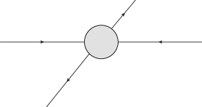
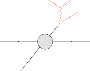
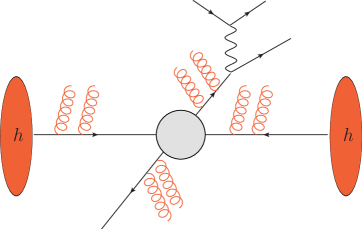
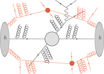
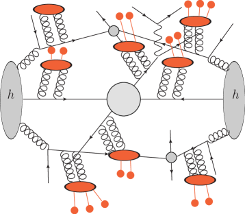
Appendix B Pair-production cross sections
The leading order parton-level cross section for QCD pair-production of particles of mass may be written in terms of scaling functions as
| (B.1) |
For heavy quark pair-production, the functions for gluon-gluon and quark-anti-quark initial states are given by [10]
| (B.2) | |||||
| (B.3) |
where and .
For the case of gluino pair-production, the equivalent functions are given by [147]
| (B.4) | |||||
where now and represents the mass-squared difference between the gluino and the -channel squark, .
For the case of scalar leptoquark pair-production, the scaling functions are given by
| (B.6) |
where . The differential cross sections with respect to the leptoquark scattering angle in the partonic centre-of-mass frame, , are given by
| (B.7) |
Appendix C The Cabibbo-Kobayashi-Maskawa matrix
The Cabibbo-Kobayashi-Maskawa (CKM) matrix (Eq. (2.55)) is a unitary matrix that can be parametrized by three mixing angles (, ) and a charge-parity (CP) violating phase, . A common choice is
| (C.4) |
where we have used the shorthand notation and . The angles have been chosen to lie in the first quadrant. Experimentally it has been observed that , so it is convenient to demonstrate the hierarchy using the Wolfenstein parametrisation:
| (C.6) |
We then have
| (C.10) |
The fit for the Wolfenstein parameters defined above gives
| (C.11) |
We can use this to estimate the CP violating phase, to be .
The Particle Data Group world average values, including errors, for the absolute values of the matrix elements of the CKM matrix are [13]:
| (C.15) |
Appendix D Supplementary material for resummation
D.1 Relation of resummation to resummation
Here we demonstrate the equivalence of transverse energy and transverse momentum resummation at . Expanding Eq. (4.83) to this order, using (4.87) and substituting into (4.81) and (4.82), we find terms involving the integrals
| (D.1) |
with . At this order, evaluating the PDFs at the scale leads to single-logarithmic terms of the same form when we use (4.89) to write
| (D.2) |
The integral (D.1) may be evaluated from
| (D.3) |
where
| (D.4) |
Writing , we have
| (D.5) |
We can safely deform the integration contour around the branch cut along the negative real axis to obtain
| (D.6) |
which, recalling that , gives
| (D.7) |
The resummed component of the transverse momentum () distribution takes the form:
| (D.8) | |||||
where ,
| (D.9) | |||||
and
| (D.10) |
Expanding to , we find the same terms as in the resummation except that (D.1) is replaced by
| (D.11) |
It therefore suffices to show that
| (D.12) |
Now corresponding to (D.4) we have
| (D.13) |
Using the result:
| (D.14) |
gives
| (D.15) |
and hence
| (D.16) |
in agreement with (D.7) and (D.12). Notice, however, that the higher () derivatives of and differ, corresponding to the difference between and resummation beyond .
D.2 Results for LHC at 7 TeV
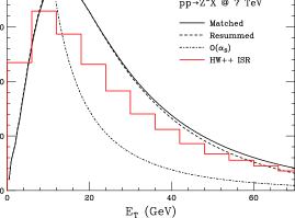
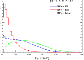
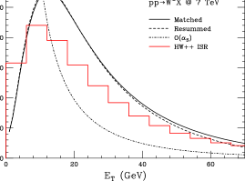
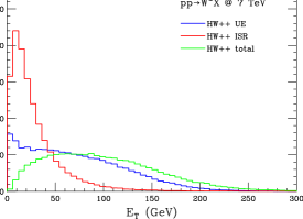
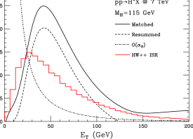
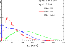
We show here results for the LHC operating at a centre-of-mass energy of 7 TeV, corresponding to those shown earlier for 14 TeV. Apart from the normalisation, the predictions for the two energies are very similar, with only a slight downward shift in the position of the peak in the distribution at the lower energy.
Appendix E Supplementary material for study
E.1 Model discrimination
The search for new physics often involves the task of discriminating between two models: one with new physics, the other without. The actual task of discovering new physics though is laborious: one has to understand the detector well enough and has to be able to obtain sufficient statistics to say with certainty that something new has been observed. Here we adopt a rather theoretical approach: we describe a purely statistical method for discriminating between models [148, 149]. This will essentially yield an upper bound on the detection reach of a heavy particle: detector effects and backgrounds will result in a reduced detection limit. It is useful, however, to be aware of the theoretical possibilities for discovery.
E.1.1 Likelihood ratios of probability density functions
Consider data points, of a mass variable measurement, . Based on these data points, a theoretical model T is times more likely than another theoretical model S, if
| (E.1) |
where is the probability of model X being true given the data set . We may use Bayes’ Theorem to rewrite as
| (E.2) |
where and are the probabilities that S and T are true respectively, called prior probabilities since they represent any previous knowledge we may possess on the theories. In the study performed here, we assume that these quantities are equal: there is no strong evidence for either model. We may simplify Eq. (E.2) further:
| (E.3) |
where we have assumed that events in the data set are independent. Eq. (E.1.1) is a discrete version of the Kullback-Leibler distance [150], a useful quantity for comparing the relative likelihood of two theories according to a given data sample. It is important to note that the distributions and are normalised to unity. This means that any difference in the number of events predicted by the two theories will not be taken into account. This will obviously underestimate the significance of a difference in the number of events as predicted by the two models, for example a substantial excess of events in an invariant mass peak that may be present. We describe a method which takes this factor into account in the next section.
E.1.2 Poisson likelihood ratios
In this modification to the method described in the previous section, we simply multiply the variable defined in Eq. (E.1) by a ratio of Poisson distributions for the total number of events:
| (E.4) |
where is the expectation value of the number of events according to theory X, given by the product of the cross section, , and the integrated luminosity, . This expression can be manipulated in a similar manner to Eq. (E.1.1) to obtain
| (E.5) |
For convenience we may define the ‘shape’ and ‘Poisson’ factors respectively:
| (E.6) |
This method takes into account the difference in the total number of events expected according to each theory at the given integrated luminosity. This is accomplished by reweighing the ‘shape’ factor by a factor which gives the ratio of probabilities to obtain the observed number of events.
E.1.3 Application to a toy model
Before applying the method to the full model, it is instructive to present its application to a simple model involving two analytical ‘toy’ distributions. Events for the two distributions have been generated by the general Monte Carlo event generation method. The ‘differential cross sections’ for the two ‘theories’ T and S with respect to a variable in arbitrary units, defined in the range , are given by
| (E.7) |
Theory T has a Gaussian peak at on top of a background falling as and theory S falls as . The situation is shown in Fig. E.1. This is qualitatively similar to the SM tail (theory S) and the SM plus a heavy particle (theory T). The ‘cross sections’ in the range are and , in arbitrary area units. Assuming an integrated ‘luminosity’ of (in equivalent arbitrary inverse area units), we have an expected number of events and . Initially, we assume that theory T is the correct underlying theory: we produce events that are actually distributed according to it. The result for the variable if theory T was ‘true’ was then found to be . This implies that theory T is 62 times more likely than theory S given this specific data set. If, however, the underlying theory is chosen to be S, then we get . This implies that in the case that theory T is ‘true’, it is easier to exclude theory S than to exclude theory T in the case that theory S is ‘true’. In other words, it is easier to make a discovery of a new resonance if it is there than to exclude it if it’s not.
E.2 The Drell-Yan cross section
In the present section we give details of the derivation of the leading order Drell-Yan cross section for , given in Eq. (5.2).
We reproduce the and couplings to fermions given in Eq. (5.1) (with ):
| (E.8) |
The propagator for a massive vector boson is given by
| (E.9) |
where is the gauge fixing parameter. Two possible gauges are , the Feynman gauge, and , the Landau gauge. Any observable quantity calculated should be independent of the gauge fixing parameter. Here we derive the differential cross section using arbitrary to show this fact explicitly. The invariant matrix element for the parton-level process (Fig. E.2) is given by
| (E.10) |
As stated in section 5.2.2, is the unit matrix when are leptons, , so we set for the allowed lepton combinations. is a CKM matrix element when (see appendix C for the CKM matrix element values). We now form:
| (E.11) | |||||
where we have defined the constant . We take the sum over the fermion spins and use the identity , where are spinors representing particles (or antiparticles) of mass , spin and 4-momentum . We have
| (E.12) | |||||
and similarly
| (E.13) | |||||
In the above, we have neglected all fermion masses. Putting everything together we obtain
| (E.14) | |||||
We can simplify Eq. (E.14) by performing the traces and contracting, using the mathematical package FORM [151]. We obtain
| (E.15) | |||||
where is the square of the quark centre-of-mass energy and . It is reassuring that the gauge-fixing parameter does not appear in Eq. (E.15), as it should not have any physical significance. We now consider the kinematics, a schematic diagram of which is shown in Fig. E.3, where for the -type quark, for the outgoing neutrino, . The angle is defined between the -type quark and the neutrino. We have and . Since we have neglected fermion masses and hence . Finally, we obtain
| (E.16) |
With these relations at hand and by using , we can rewrite as
| (E.17) | |||||
We have averaged over initial spins by multiplying by and divided by to account for the fact that the fusing quark and anti-quark must form a colour singlet. We have also summed over all possible quark flavour combinations, . Using Eq. (E.17) we may now write the total matrix element squared as . It is not difficult to see that we may group the -even and -odd terms into the functions and , defined in Eqs. (5.3) and (5.4) respectively.
If the collision had involved only quarks of constant centre-of-mass energy then we would simply plug the matrix element squared at parton level into the expression for the scattering differential cross section:
| (E.18) |
Integrating over would give
| (E.19) |
In a collision which involves a quark and an anti-quark , each can come from either of the two hadrons. Let us identify the two hadrons to ‘left’ (hadron A) when moving in the positive -direction and ‘right’ (hadron B) when moving in the negative -direction. Since we do not have any information about which quark came from which hadron, we have to include both possibilities in the calculation. If the quark comes from hadron A, and the anti-quark comes from hadron B then the definition of the angle , and hence , remains unchanged. Contrariwise, if comes from A and comes from B, we have to take in our expressions to take into account the fact that the -axis definition would change. A schematic diagram can be seen in Fig. E.4.
Consider the prior case first. Note that if we consider the lab frame collision of the quarks, where and , we may write as , where is the hadron centre-of-mass collision energy. The quarks are of course confined in the hadrons and possess a distribution of momenta, distinct for each quark flavour. We denote the differential cross section by and the full hadronic differential cross section, including the PDFs, by . To obtain the full hadronic differential cross section we multiply by the parton density functions, and integrate over the momentum fractions and , using a delta function which ensures that the quarks have the correct centre-of-mass energy, . For the case of coming A and from B:
If we now consider the case when the comes from B and from A, we have to take . This will not change the -even factor, but will change the -odd factor:
To combine the two results into the full differential cross section, we combine the PDFs into an even and an odd function respectively:
| (E.22) |
This results in the following expression:
Since , we have and by defining the boson (or dilepton) rapidity , we finally arrive at the full hadronic differential cross section:
| (E.24) |
where we have set . This is exactly what was given in section 5.2.2, Eq. (5.2).
Appendix F Supplementary material for leptoquark study
F.1 Feynman rules and diagrams
The Feynman rules [132] relevant to the leptoquark pair-production diagrams are given in Figs. F.1 and F.2. The relevant parton-level Feynman diagrams are shown in Figs. F.3 and F.4 for gluon-gluon and quark-anti-quark initial states respectively.

|

|


Since the couplings to light generations are suppressed in the kind of models we are considering, leptoquark single-production in hadron colliders can proceed only via -quark gluon fusion, as shown in Fig. F.5. However this is also heavily suppressed due to the low -quark PDF and the small couplings to fermions, and can be neglected.

F.2 The effective Lagrangian for derivatively-coupled leptoquarks
The Lagrangian for derivatively-coupled conjugate fields, which appears in Eq. (LABEL:eq:lagd), also contains terms involving the conjugate fields, such as
| (F.1) |
To manipulate the above expression for the case of on-shell decays as we did in Eq. (5.41), we need to show that
| (F.2) |
where is a 4-component spinor and . This can be demonstrated by using the following identities [152]:
| (F.3) |
and hence
| (F.4) |
So the necessary effective Lagrangian for the decay is given by
| (F.5) |
The full list of effective Lagrangians for the primed leptoquarks, from which the decay modes and couplings in Tables 5.4 and 5.6 can be derived, is given by
| (F.6) | |||||
| (F.7) | |||||
| (F.8) | |||||
| (F.9) | |||||
| (F.10) | |||||
where we have defined: (and equivalent definitions for ) and . We have also used the fact that the doublet leptoquarks may be written as a vector . We have set the quark and lepton couplings to equal, ,111The implementation in H ERWIG++ version 2.5.0 also includes this simplification. however these can be reinstated trivially by replacing where a quark mass term appears and where a lepton mass term appears.
Note that terms appearing in this Lagrangian are no longer gauge-invariant. This is consistent since these terms would appear in the Lagrangian after electroweak symmetry breaking and vanish as the fermion masses tend to zero. The Lagrangian is, of course, gauge-invariant.
F.3 reconstruction method
In terms of the momentum ratios defined in Eq. (5.3.4.1), the conditions for balancing the total missing transverse momentum can be written as
| (F.11) | |||||
| (F.12) |
The mass-shell conditions, except for , can be written as
| (F.13) | |||||
| (F.14) | |||||
| (F.15) | |||||
| (F.16) |
where is the reconstructed mass of the hadronic top and is the assumed mass of the semi-leptonic top. By eliminating and from Eqs. (F.11), (F.15) and (F.16), one obtains
| (F.17) |
where
| (F.18) | |||||
| (F.19) |
Using a vector , Eqs. (F.12), (F.13), (F.14) and (F.17) can be recasted as
| (F.20) |
where
| (F.25) |
and
| (F.27) |
and are defined as
| (F.28) | |||||
| (F.29) |
From Eq. (F.20), we can determine as a function of . Finally, can be determined from the mass-shell condition:
| (F.30) |
This provides a quartic equation for , and we can find up to four real solutions in the physical range . We can then obtain by substituting into Eq. (F.16).
F.4 reconstruction method
Given in Eq. (5.3.6.1), can be minimised in terms of . The result is
| (F.31) | |||||
where
| (F.32) |
and is the transverse mass of the system. This allows us to calculate by one-parameter minimisation:
| (F.33) |
Since is a monotonically increasing function of , if :
| (F.34) |
Furthermore, since there exists a value which fulfils , we find
| (F.35) |
If , we have to search for other values of . For the true and , say and , we have
| (F.36) |
This assures existence of which satisfies the relation . By scanning from 0 to , one finds:
| (F.37) |
and
| (F.38) |
Hence we have
| (F.39) |
References
- [1] A. Papaefstathiou and B. Webber, “Effects of QCD radiation on inclusive variables for determining the scale of new physics at hadron colliders,” JHEP 0906 (2009) 069, 0903.2013.
- [2] A. Papaefstathiou and B. Webber, “Effects of invisible particle emission on global inclusive variables at hadron colliders,” JHEP 1007 (2010) 018, 1004.4762.
- [3] A. Papaefstathiou, J. M. Smillie, and B. R. Webber, “Resummation of transverse energy in vector boson and Higgs boson production at hadron colliders,” JHEP 1004 (2010) 084, 1002.4375.
- [4] A. Papaefstathiou and O. Latunde-Dada, “NLO production of W-prime bosons at hadron colliders using the MC@NLO and POWHEG methods,” JHEP 0907 (2009) 044, 0901.3685.
- [5] B. Gripaios, A. Papaefstathiou, K. Sakurai, and B. Webber, “Searching for third-generation composite leptoquarks at the LHC,” JHEP 1101 (2011) 156, 1010.3962.
- [6] R. P. Feynman, “QED: The Strange Theory of Light and Matter,” Penguin (1990).
- [7] C. Burgess and G. Moore, “The Standard Model: A Primer,” Cambridge (2007).
- [8] M. Peskin and D. Schroeder, “An Introdution to Quantum Field Theory,” Westview Press (1995).
- [9] M. Seymour, “Quantum ChromoDynamics,” 1010.2330.
- [10] R. K. Ellis, W. J. Stirling, and B. R. Webber, “QCD and Collider Physics,” Cambridge (1996).
- [11] J. Donoghue, E. Golowich, and B. Holstein, “Dynamics of the Standard Model,” Cambridge (1992).
- [12] S. Pokorski, “Gauge Field Theories,” Cambridge (2000).
- [13] Nakamura, K. et al., “Review of particle physics,” J. Phys. G G37 (2010) 075021.
- [14] Nobelprize.org, “Nobel Prize in Physics 2008.” http://nobelprize.org/nobel_prizes/physics/laureates/2008/.
- [15] R. Barbieri and A. Strumia, “What is the limit on the Higgs mass?,” Phys.Lett. B462 (1999) 144–149, hep-ph/9905281.
- [16] WMAP Collaboration Collaboration, D. Spergel et al., “Wilkinson Microwave Anisotropy Probe (WMAP) three year results: implications for cosmology,” Astrophys.J.Suppl. 170 (2007) 377, astro-ph/0603449.
- [17] MACHO Collaboration, C. Alcock et al., “The MACHO project: Microlensing results from 5.7 years of LMC observations,” Astrophys. J. 542 (2000) 281–307, astro-ph/0001272.
- [18] A. R. Raklev, “Massive Metastable Charged (S)Particles at the LHC,” Mod.Phys.Lett. A24 (2009) 1955–1969, 0908.0315.
- [19] J. R. Ellis, A. R. Raklev, and O. K. Oye, “Gravitino dark matter scenarios with massive metastable charged sparticles at the LHC,” JHEP 0610 (2006) 061, hep-ph/0607261.
- [20] S. Dimopoulos, “LHC, SSC and the universe,” Phys.Lett. B246 (1990) 347–352.
- [21] M. Dine, “Supersymmetry and String Theory: Beyond the Standard Model,” Cambridge (2007).
- [22] M. Bustamante, L. Cieri, and J. Ellis, “Beyond the Standard Model for Montaneros,” 0911.4409.
- [23] R. Mohapatra, “Unification and Supersymmetry: The Frontiers of Quark-Lepton Physics,” Springer (2003).
- [24] S. P. Martin, “A Supersymmetry primer,” hep-ph/9709356.
- [25] S. Krippendorf, F. Quevedo, and O. Schlotterer, “Cambridge Lectures on Supersymmetry and Extra Dimensions,” 1011.1491.
- [26] T. Appelquist, H.-C. Cheng, and B. A. Dobrescu, “Bounds on universal extra dimensions,” Phys.Rev. D64 (2001) 035002, hep-ph/0012100.
- [27] L. Randall and R. Sundrum, “A Large mass hierarchy from a small extra dimension,” Phys.Rev.Lett. 83 (1999) 3370–3373, hep-ph/9905221.
- [28] A. Fitzpatrick, G. Perez, and L. Randall, “Flavor from Minimal Flavor Violation and a Viable Randall-Sundrum Model,” 0710.1869.
- [29] R. Foadi, M. T. Frandsen, T. A. Ryttov, and F. Sannino, “Minimal Walking Technicolor: Set Up for Collider Physics,” Phys.Rev. D76 (2007) 055005, 0706.1696.
- [30] M. Antola, K. Tuominen, F. Sannino, and S. Di Chiara, “Perturbative minimal superconformal technicolor,” J.Phys.Conf.Ser. 259 (2010) 012054.
- [31] N. Arkani-Hamed, A. G. Cohen, and H. Georgi, “(De)constructing dimensions,” Phys.Rev.Lett. 86 (2001) 4757–4761, hep-th/0104005.
- [32] N. Arkani-Hamed, A. G. Cohen, and H. Georgi, “Electroweak symmetry breaking from dimensional deconstruction,” Phys.Lett. B513 (2001) 232–240, hep-ph/0105239.
- [33] M. Perelstein, “Little Higgs models and their phenomenology,” Prog.Part.Nucl.Phys. 58 (2007) 247–291, hep-ph/0512128.
- [34] H.-C. Cheng and I. Low, “TeV symmetry and the little hierarchy problem,” JHEP 0309 (2003) 051, hep-ph/0308199.
- [35] M. Perelstein, “Little Higgs models and T parity,” Pramana 67 (2006) 813–820, hep-ph/0703138.
- [36] H. Sahlmann, “Loop quantum gravity - a short review,” 1001.4188.
- [37] montecarloresort.com, “Monte Carlo Resort.” http://en.montecarloresort.com/.
- [38] A. Buckley, J. Butterworth, S. Gieseke, D. Grellscheid, S. Hoche, et al., “General-purpose event generators for LHC physics,” 1101.2599.
- [39] J. E. Huth, N. Wainer, K. Meier, N. Hadley, F. Aversa, et al., “Toward a standardization of jet definitions,”.
- [40] G. P. Salam, “Towards Jetography,” Eur.Phys.J. C67 (2010) 637–686, 0906.1833.
- [41] Axial Field Spectrometer Collaboration Collaboration, T. Akesson et al., “Double parton scattering in pp collisions at S**(1/2) = 63-GeV,” Z.Phys. C34 (1987) 163.
- [42] UA5 Collaboration Collaboration, G. Alner et al., “The UA5 High-Energy anti-p p Simulation Program,” Nucl.Phys. B291 (1987) 445.
- [43] J. Butterworth, J. R. Forshaw, and M. Seymour, “Multiparton interactions in photoproduction at HERA,” Z.Phys. C72 (1996) 637–646, hep-ph/9601371.
- [44] M. Bahr, S. Gieseke, and M. H. Seymour, “Simulation of multiple partonic interactions in Herwig++,” JHEP 0807 (2008) 076, 0803.3633.
- [45] T. Sjostrand, S. Mrenna, and P. Z. Skands, “A Brief Introduction to PYTHIA 8.1,” Comput.Phys.Commun. 178 (2008) 852–867, 0710.3820.
- [46] M. Bahr, S. Gieseke, M. Gigg, D. Grellscheid, K. Hamilton, et al., “Herwig++ Physics and Manual,” Eur.Phys.J. C58 (2008) 639–707, 0803.0883.
- [47] T. Gleisberg et al., “Event generation with SHERPA 1.1,” JHEP 02 (2009) 007, 0811.4622.
- [48] “The Herwig++ event generator.” http://projects.hepforge.org/herwig/.
- [49] G. Marchesini and B. Webber, “Monte Carlo Simulation of General Hard Processes with Coherent QCD Radiation,” Nucl.Phys. B310 (1988) 461.
- [50] L. Lonnblad, “ThePEG, Pythia7, Herwig++ and Ariadne,” Nucl.Instrum.Meth. A559 (2006) 246–248.
- [51] J. Alwall, A. Ballestrero, P. Bartalini, S. Belov, E. Boos, et al., “A Standard format for Les Houches event files,” Comput.Phys.Commun. 176 (2007) 300–304, hep-ph/0609017.
- [52] S. Gieseke, P. Stephens, and B. Webber, “New formalism for QCD parton showers,” JHEP 0312 (2003) 045, hep-ph/0310083.
- [53] S. Gieseke, D. Grellscheid, K. Hamilton, A. Papaefstathiou, S. Platzer, et al., “Herwig++ 2.5 Release Note,” 1102.1672.
- [54] B. Allanach, C. Balazs, G. Belanger, M. Bernhardt, F. Boudjema, et al., “SUSY Les Houches Accord 2,” Comput.Phys.Commun. 180 (2009) 8–25, 0801.0045.
- [55] S. Frixione and B. R. Webber, “Matching NLO QCD computations and parton shower simulations,” JHEP 0206 (2002) 029, hep-ph/0204244.
- [56] S. Frixione, F. Stoeckli, P. Torrielli, B. R. Webber, and C. D. White, “The MCaNLO 4.0 Event Generator,” 1010.0819.
- [57] P. Nason, “A New method for combining NLO QCD with shower Monte Carlo algorithms,” JHEP 0411 (2004) 040, hep-ph/0409146.
- [58] S. Frixione, P. Nason, and C. Oleari, “Matching NLO QCD computations with Parton Shower simulations: the POWHEG method,” JHEP 0711 (2007) 070, 0709.2092.
- [59] O. Latunde-Dada, “Simulations of QCD processes at High Energy Colliders.,” University of Cambridge, http://www.hep.phy.cam.ac.uk/theory/seyi/thesis (2008).
- [60] J. R. Forshaw, J. F. Gunion, L. Hodgkinson, A. Papaefstathiou, and A. D. Pilkington, “Reinstating the ’no-lose’ theorem for NMSSM Higgs discovery at the LHC,” JHEP 04 (2008) 090, 0712.3510.
- [61] ATLAS Collaboration Collaboration, E. Bouhova-Thacker et al., “Expected performance of vertex reconstruction in the ATLAS experiment at the LHC,” IEEE Trans.Nucl.Sci. 57 (2010) 760–767.
- [62] A. J. Barr and C. G. Lester, “A Review of the Mass Measurement Techniques proposed for the Large Hadron Collider,” J.Phys.G G37 (2010) 123001, 1004.2732.
- [63] I. Hinchliffe, F. Paige, M. Shapiro, J. Soderqvist, and W. Yao, “Precision SUSY measurements at CERN LHC,” Phys.Rev. D55 (1997) 5520–5540, hep-ph/9610544.
- [64] F. E. Paige, “Supersymmetry signatures at the CERN LHC,” hep-ph/9801254.
- [65] D. Tovey, “Measuring the SUSY mass scale at the LHC,” Phys.Lett. B498 (2001) 1–10, hep-ph/0006276.
- [66] G. Bozzi, S. Catani, D. de Florian, and M. Grazzini, “Higgs boson production at the LHC: Transverse-momentum resummation and rapidity dependence,” Nucl.Phys. B791 (2008) 1–19, 0705.3887. This paper is dedicated to the memory of Jiro Kodaira, great friend and distinguished colleague.
- [67] G. Bozzi, S. Catani, G. Ferrera, D. de Florian, and M. Grazzini, “Transverse-momentum resummation: A Perturbative study of Z production at the Tevatron,” Nucl.Phys. B815 (2009) 174–197, 0812.2862.
- [68] S. Mantry and F. Petriello, “Factorization and Resummation of Higgs Boson Differential Distributions in Soft-Collinear Effective Theory,” Phys.Rev. D81 (2010) 093007, 0911.4135.
- [69] P. Konar, K. Kong, and K. T. Matchev, “hat-s(min)**(1/2): A Global inclusive variable for determining the mass scale of new physics in events with missing energy at hadron colliders,” JHEP 0903 (2009) 085, 0812.1042.
- [70] P. Konar, K. Kong, K. T. Matchev, and M. Park, “RECO level sqrt s_min and subsystem sqrt s_min: Improved global inclusive variables for measuring the new physics mass scale in missing E_T events at hadron colliders,” 1006.0653.
- [71] A. Martin, W. Stirling, R. Thorne, and G. Watt, “Parton distributions for the LHC,” Eur.Phys.J. C63 (2009) 189–285, 0901.0002.
- [72] A. Vogt, “Efficient evolution of unpolarized and polarized parton distributions with QCD-PEGASUS,” Comput. Phys. Commun. 170 (2005) 65–92, hep-ph/0408244.
- [73] J. Abate and P. Valko, “Multi-precision Laplace transform inversion,” International Journal for Numerical Methods in Engineering 60 (2004) 979–993.
- [74] R. Brent, “Algorithms for Minimization without Derivatives,” Prentice-Hall (1973).
- [75] M. Galassi, K. Davies, J. Theiler, J. Gough, G. Jungman, P. Alken, M. Booth, and F. Rossi, “GNU Scientific Library Reference Manual (3rd Ed.),” Network Theory Ltd (2009).
- [76] F. Hubaut, E. Monnier, P. Pralavorio, K. Smolek, and V. Simak, “ATLAS sensitivity to top quark and W boson polarization in t anti-t events,” Eur.Phys.J. C44S2 (2005) 13–33, hep-ex/0508061. ATLAS scientific note SN-ATLAS-2005-052.
- [77] The ATLAS Collaboration Collaboration, G. Aad et al., “Expected Performance of the ATLAS Experiment - Detector, Trigger and Physics,” 0901.0512.
- [78] A. Sherstnev and R. Thorne, “Parton Distributions for LO Generators,” Eur.Phys.J. C55 (2008) 553–575, 0711.2473.
- [79] A. Sherstnev and R. Thorne, “Different PDF approximations useful for LO Monte Carlo generators,” 0807.2132.
- [80] B. Allanach, M. Battaglia, G. Blair, M. S. Carena, A. De Roeck, et al., “The Snowmass points and slopes: Benchmarks for SUSY searches,” Eur.Phys.J. C25 (2002) 113–123, hep-ph/0202233.
- [81] ATLAS Collaboration Collaboration, G. Aad et al., “Measurements of underlying-event properties using neutral and charged particles in pp collisions at 900 GeV and 7 TeV with the ATLAS detector at the LHC,” 1103.1816.
- [82] Y. L. Dokshitzer, D. Diakonov, and S. Troian, “Hard Processes in Quantum Chromodynamics,” Phys.Rept. 58 (1980) 269–395.
- [83] G. Parisi and R. Petronzio, “Small Transverse Momentum Distributions in Hard Processes,” Nucl.Phys. B154 (1979) 427.
- [84] G. Curci, M. Greco, and Y. Srivastava, “QCD jets from coherent states,” Nucl.Phys. B159 (1979) 451.
- [85] A. Bassetto, M. Ciafaloni, and G. Marchesini, “Inelastic Distributions and Color Structure in Perturbative QCD,” Nucl.Phys. B163 (1980) 477.
- [86] J. Kodaira and L. Trentadue, “Summing Soft Emission in QCD,” Phys.Lett. B112 (1982) 66.
- [87] J. Kodaira and L. Trentadue, “Single Logarithm Effects in electron-Positron Annihilation,” Phys.Lett. B123 (1983) 335.
- [88] J. C. Collins, D. E. Soper, and G. F. Sterman, “Transverse Momentum Distribution in Drell-Yan Pair and W and Z Boson Production,” Nucl.Phys. B250 (1985) 199.
- [89] F. Halzen, A. D. Martin, D. Scott, and M. Tuite, “The transverse hadronic energy accompanying weak bosons,” Z.Phys. C14 (1982) 351.
- [90] C. Davies and B. Webber, “Transverse hadronic energy emission in hard scattering processes,” Z.Phys. C24 (1984) 133.
- [91] G. Altarelli, G. Martinelli, and F. Rapuano, “The transverse hadronic energy in W and Z0 production,” Z.Phys. C32 (1986) 369–375.
- [92] G. Corcella, I. Knowles, G. Marchesini, S. Moretti, K. Odagiri, et al., “HERWIG 6: An Event generator for hadron emission reactions with interfering gluons (including supersymmetric processes),” JHEP 0101 (2001) 010, hep-ph/0011363.
- [93] S. Catani, D. de Florian, and M. Grazzini, “Universality of nonleading logarithmic contributions in transverse momentum distributions,” Nucl.Phys. B596 (2001) 299–312, hep-ph/0008184.
- [94] I. W. Stewart, F. J. Tackmann, and W. J. Waalewijn, “The Beam Thrust Cross Section for Drell-Yan at NNLL Order,” Phys.Rev.Lett. 106 (2011) 032001, 1005.4060.
- [95] C. Davies and W. Stirling, “Nonleading Corrections to the Drell-Yan Cross-Section at Small Transverse Momentum,” Nucl.Phys. B244 (1984) 337.
- [96] C. Balazs, J.-w. Qiu, and C. Yuan, “Effects of QCD resummation on distributions of leptons from the decay of electroweak vector bosons,” Phys.Lett. B355 (1995) 548–554, hep-ph/9505203.
- [97] S. Catani, E. D’Emilio, and L. Trentadue, “The gluon form-factor to higher orders: gluon gluon annihilation at small Q-transverse,” Phys.Lett. B211 (1988) 335–342.
- [98] D. de Florian and M. Grazzini, “Next-to-next-to-leading logarithmic corrections at small transverse momentum in hadronic collisions,” Phys.Rev.Lett. 85 (2000) 4678–4681, hep-ph/0008152.
- [99] D. de Florian and M. Grazzini, “The Structure of large logarithmic corrections at small transverse momentum in hadronic collisions,” Nucl.Phys. B616 (2001) 247–285, hep-ph/0108273.
- [100] R. Kauffman, “Higher order corrections to Higgs boson p(T),” Phys.Rev. D45 (1992) 1512–1517.
- [101] P. Langacker, “The Physics of Heavy Z-prime Gauge Bosons,” Rev.Mod.Phys. 81 (2009) 1199–1228, 0801.1345.
- [102] R. N. Mohapatra and J. C. Pati, “Left-Right Gauge Symmetry and an Isoconjugate Model of CP Violation,” Phys.Rev. D11 (1975) 566–571.
- [103] F. Pisano and V. Pleitez, “An SU(3) x U(1) model for electroweak interactions,” Phys.Rev. D46 (1992) 410–417, hep-ph/9206242.
- [104] H.-C. Cheng, K. T. Matchev, and M. Schmaltz, “Bosonic supersymmetry? Getting fooled at the CERN LHC,” Phys.Rev. D66 (2002) 056006, hep-ph/0205314.
- [105] C. T. Hill and E. H. Simmons, “Strong dynamics and electroweak symmetry breaking,” Phys.Rept. 381 (2003) 235–402, hep-ph/0203079.
- [106] R. S. Chivukula, H.-J. He, J. Howard, and E. H. Simmons, “The Structure of electroweak corrections due to extended gauge symmetries,” Phys.Rev. D69 (2004) 015009, hep-ph/0307209.
- [107] O. Latunde-Dada and A. Papaefstathiou, “Wpnlo homepage.” http://www.hep.phy.cam.ac.uk/theory/andreas/wpnlo.
- [108] T. G. Rizzo, “The Determination of the Helicity of W’ Boson Couplings at the LHC,” JHEP 0705 (2007) 037, 0704.0235.
- [109] B. Fuks, M. Klasen, F. Ledroit, Q. Li, and J. Morel, “Precision predictions for Z-prime - production at the CERN LHC: QCD matrix elements, parton showers, and joint resummation,” Nucl.Phys. B797 (2008) 322–339, 0711.0749.
- [110] G. Altarelli, B. Mele, and M. Ruiz-Altaba, “Searching for new heavy vector bosons in p anti-p colliders,” Z.Phys. C45 (1989) 109.
- [111] D. Berdine, N. Kauer, and D. Rainwater, “Breakdown of the Narrow Width Approximation for New Physics,” Phys.Rev.Lett. 99 (2007) 111601, hep-ph/0703058.
- [112] O. Latunde-Dada, “Herwig++ Monte Carlo At Next-To-Leading Order for e+e- annihilation and lepton pair production,” JHEP 0711 (2007) 040, 0708.4390.
- [113] CDF Collaboration Collaboration, A. Abulencia et al., “Search for W-prime boson decaying to electron-neutrino pairs in p anti-p collisions at s**(1/2) = 1.96-TeV,” Phys.Rev. D75 (2007) 091101, hep-ex/0611022.
- [114] D0 Collaboration Collaboration, V. Abazov et al., “Search for W-prime bosons decaying to an electron and a neutrino with the D0 detector,” Phys.Rev.Lett. 100 (2008) 031804, 0710.2966.
- [115] D0 Collaboration Collaboration, V. Abazov et al., “Search for W-prime boson production in the top quark decay channel,” Phys.Lett. B641 (2006) 423–431, hep-ex/0607102.
- [116] D0 Collaboration Collaboration, V. Abazov et al., “Search for W-prime Boson Resonances Decaying to a Top Quark and a Bottom Quark,” Phys.Rev.Lett. 100 (2008) 211803, 0803.3256.
- [117] CDF Collaboration Collaboration, T. Aaltonen et al., “Search for the Production of Narrow t anti-b Resonances in 1.9 fb-1 of p anti-p Collisions at s**(1/2) = 1.96-TeV,” Phys.Rev.Lett. 103 (2009) 041801, 0902.3276.
- [118] A. Duperrin, “Review of searches for Higgs bosons and beyond the standard model physics at the Tevatron,” Eur.Phys.J. C59 (2009) 297–334, 0805.3624.
- [119] T. A. Collaboration, “Search for high-mass states with one lepton plus missing transverse momentum in proton-proton collisions at sqrt(s) = 7 TeV with the ATLAS detector,” 1103.1391.
- [120] Y. Zhang, H. An, X. Ji, and R. Mohapatra, “Right-handed quark mixings in minimal left-right symmetric model with general CP violation,” Phys.Rev. D76 (2007) 091301, 0704.1662.
- [121] P. Langacker and S. Uma Sankar, “Bounds on the Mass of W(R) and the W(L)-W(R) Mixing Angle xi in General SU(2)-L x SU(2)-R x U(1) Models,” Phys.Rev. D40 (1989) 1569–1585.
- [122] CTEQ Collaboration Collaboration, H. Lai et al., “Global QCD analysis of parton structure of the nucleon: CTEQ5 parton distributions,” Eur.Phys.J. C12 (2000) 375–392, hep-ph/9903282.
- [123] A. D. Martin, R. Roberts, W. Stirling, and R. Thorne, “MRST2001: Partons and alpha(s) from precise deep inelastic scattering and Tevatron jet data,” Eur.Phys.J. C23 (2002) 73–87, hep-ph/0110215.
- [124] CDF Collaboration Collaboration, A. A. Affolder et al., “The Transverse momentum and total cross-section of e+ e- pairs in the Z-boson region from p anti-p collisions at S**(1/2) = 1.8-TeV,” Phys.Rev.Lett. 84 (2000) 845–850, hep-ex/0001021.
- [125] D. B. Kaplan, “Flavor at SSC energies: A New mechanism for dynamically generated fermion masses,” Nucl.Phys. B365 (1991) 259–278. Revised version.
- [126] B. Gripaios, “Composite Leptoquarks at the LHC,” JHEP 1002 (2010) 045, 0910.1789.
- [127] S. Davidson and S. Descotes-Genon, “Minimal Flavour Violation for Leptoquarks,” 1009.1998.
- [128] D0 Collaboration, V. M. Abazov et al., “Search for third generation scalar leptoquarks decaying into ,” Phys. Rev. Lett. 101 (2008) 241802, 0806.3527.
- [129] D0 Collaboration, V. M. Abazov et al., “Search for third-generation leptoquarks in collisions at = 1.96-TeV,” Phys. Rev. Lett. 99 (2007) 061801, 0705.0812.
- [130] T. Sjostrand, S. Mrenna, and P. Z. Skands, “PYTHIA 6.4 Physics and Manual,” JHEP 05 (2006) 026, hep-ph/0603175.
- [131] T. Sjostrand, “PYTHIA 8 Status Report,” 0809.0303.
- [132] J. Blumlein, E. Boos, and A. Kryukov, “Leptoquark pair production in hadronic interactions,” Z. Phys. C76 (1997) 137–153, hep-ph/9610408.
- [133] A. Belyaev, C. Leroy, R. Mehdiyev, and A. Pukhov, “Leptoquark single and pair production at LHC with CalcHEP/CompHEP in the complete model,” JHEP 0509 (2005) 005, hep-ph/0502067.
- [134] C. Lester and D. Summers, “Measuring masses of semiinvisibly decaying particles pair produced at hadron colliders,” Phys.Lett. B463 (1999) 99–103, hep-ph/9906349.
- [135] S. Ovyn, X. Rouby, and V. Lemaitre, “DELPHES, a framework for fast simulation of a generic collider experiment,” 0903.2225.
- [136] M. Serna, “A Short comparison between m(T2) and m(CT),” JHEP 0806 (2008) 004, 0804.3344.
- [137] H.-C. Cheng and Z. Han, “Minimal Kinematic Constraints and m(T2),” JHEP 0812 (2008) 063, 0810.5178.
- [138] A. J. Barr, B. Gripaios, and C. G. Lester, “Transverse masses and kinematic constraints: from the boundary to the crease,” JHEP 0911 (2009) 096, 0908.3779.
- [139] M. L. Mangano, M. Moretti, F. Piccinini, R. Pittau, and A. D. Polosa, “ALPGEN, a generator for hard multiparton processes in hadronic collisions,” JHEP 0307 (2003) 001, hep-ph/0206293.
- [140] J. Shelton, “Polarized tops from new physics: signals and observables,” Phys.Rev. D79 (2009) 014032, 0811.0569.
- [141] R. M. Godbole, S. D. Rindani, and R. K. Singh, “Lepton distribution as a probe of new physics in production and decay of the t quark and its polarization,” JHEP 0612 (2006) 021, hep-ph/0605100.
- [142] R. Dalitz and G. R. Goldstein, “The Decay and polarization properties of the top quark,” Phys.Rev. D45 (1992) 1531–1543.
- [143] M. Guchait and D. Roy, “Using Tau Polarization for Charged Higgs Boson and SUSY Searches at LHC,” 0808.0438.
- [144] R. Godbole, M. Guchait, and D. Roy, “Using Tau Polarization to probe the Stau Co-annihilation Region of mSUGRA Model at LHC,” Phys.Rev. D79 (2009) 095015, 0807.2390.
- [145] I. Low, R. Rattazzi, and A. Vichi, “Theoretical Constraints on the Higgs Effective Couplings,” JHEP 1004 (2010) 126, 0907.5413.
- [146] B. Gripaios, A. Pomarol, F. Riva, and J. Serra, “Beyond the Minimal Composite Higgs Model,” JHEP 0904 (2009) 070, 0902.1483.
- [147] W. Beenakker, R. Hopker, M. Spira, and P. Zerwas, “Gluino pair production at the Tevatron,” Z.Phys. C69 (1995) 163–166, hep-ph/9505416.
- [148] C. Athanasiou, C. G. Lester, J. M. Smillie, and B. R. Webber, “Distinguishing Spins in Decay Chains at the Large Hadron Collider,” JHEP 0608 (2006) 055, hep-ph/0605286.
- [149] O. Latunde-Dada, “Determining Properties of New Fundamental Particles at the Large Hadron Collider.,” University of Cambridge, http://www.hep.phy.cam.ac.uk/atlas/susydoc/smillie_thesis.pdf (2007).
- [150] S. Kullback and R. Leibler, “On information and sufficiency,” Annals of Mathematical Statistics 22(1) (1951).
- [151] J. Vermaseren, “New features of FORM,” math-ph/0010025.
- [152] H. K. Dreiner, H. E. Haber, and S. P. Martin, “Two-component spinor techniques and Feynman rules for quantum field theory and supersymmetry,” Phys.Rept. 494 (2010) 1–196, 0812.1594.