SLAC–PUB–14549 August, 2011

Constructing Amplitudes from Their Soft Limits

Camille Boucher-Veronneauand Andrew J. Larkoski

SLAC, Menlo Park, CA 94025

ABSTRACT

The existence of universal soft limits for gauge-theory and gravity amplitudes has been known for a long time. The properties of the soft limits have been exploited in numerous ways; in particular for relating an $n$-point amplitude to an $(n-1)$-point amplitude by removing a soft particle. Recently, a procedure called inverse soft was developed by which “soft” particles can be systematically added to an amplitude to construct a higher-point amplitude for generic kinematics. We review this procedure and relate it to Britto-Cachazo-Feng-Witten recursion. We show that all tree-level amplitudes in gauge theory and gravity up through seven points can be constructed in this way, as well as certain classes of NMHV gauge-theory amplitudes with any number of external legs. This provides us with a systematic procedure for constructing amplitudes solely from their soft limits.

1 Introduction

In the last twenty years, we have seen a resurgence of interest in the S-matrix program of the 60’s [1] whose goal was to define a quantum field theory through the analytic properties of its S-matrix. The unitarity [2] and generalized unitarity [3] methods dramatically simplified loop-level calculations. At tree level, recent interest was triggered in part by Witten’s remarkable description of gauge theory as a string theory in twistor space [4]. Detailed studies of an amplitude’s analytic properties have led, in particular, to the Britto-Cachazo-Feng-Witten (BCFW) recursion relations [5, 6]. These relations exploit the analyticity of the amplitudes in a distinct way from the old S-matrix program: external particles’ momenta are deformed by a complex parameter and the factorization channels of the deformed amplitude are studied. This procedure leads to very compact, on-shell, recursion formulas which have been solved in generality for ${\cal N}=4$ sYM [7].

In the 1980’s, it was noticed that photon radiation amplitudes could be expressed as products of soft factors times a lower-point amplitude [8]. A recent advancement in this area due to Arkani-Hamed, et al., is a method called inverse soft which attempts to construct amplitudes from their soft limits alone [9, 10, 11]. Inverse soft was motivated by studying the residues of poles in the Grassmannian of [9]. The Grassmannian has been conjectured to produce all leading singularities [12] in planar ${\cal N}=4$ sYM from the residues of its poles. The relationship between leading singularities at different loop orders, numbers of external legs and helicity configurations was studied using inverse soft in [13]. In addition, it has been shown that inverse soft reproduces tree-level maximally-helicity-violating (MHV) amplitudes and six-point next-to-MHV (NMHV) amplitudes in ${\cal N}=4$ sYM [10].

In [14], inverse soft was shown to reproduce MHV gravity amplitudes in the form first given in [15]. Very recently, inspired in part by the inverse-soft procedure discussed in [14], Hodges presented new expressions for MHV amplitudes [16]. However, other than this result, the application of inverse soft to gravity amplitudes has been minimal. This is (possibly) due to several factors: gravity lacks a color expansion (and hence color ordering) and the Planck mass is dimensionful. Moreover, the gravity soft factor is a gauge-invariant sum of many terms and the inverse-soft procedure exploits each term individually. Thus, there is not a unique form for the gravity soft factor and so there is not a unique procedure for inverse soft in gravity. Here, we wish to put inverse soft on a firmer ground for gravity amplitudes, as well as reviewing its application to gauge theory amplitudes.

The main result of this paper is to extend the applicability of inverse soft for gauge theory and gravity amplitudes from MHV to NMHV. The gravity soft factor in [14] cannot easily reproduce multiparticle factorization channels necessary to construct NMHV amplitudes. We find that its most natural generalization that can do so is a soft factor inspired by BCFW. We will use inverse soft to re-express terms in the BCFW expansion of an $n$-point amplitude $A_{n}$ as a sum of products of soft factors times a lower point amplitude $A_{n-m}$.

For gauge theory we have

$$A_{n}=\sum_{m=1}^{m_{\text{max}}}\sum_{j=1}^{2}\biggl{(}\prod_{i=1}^{m}{\cal S^{\prime}}(p_{i,j})\biggr{)}A^{\prime}_{n-m}(\overline{p}_{i,j})\ ,$$ (1)

where ${\cal S}$ is a gauge-theory soft factor. Here, $m$ ranges over the possible BCFW terms; $m=1$ are the two-particle factorization terms, $m=2$ the three-particle terms, etc., and $p_{i,j}$ represent appropriate particles added to the amplitude in the inverse-soft construction. The lower-point amplitude $A_{n-m}(\overline{p}_{i,j})$ is the $(n-m)$-point amplitude where particles $p_{i,j}$ were removed from $A_{n}$. The maximum value of $m$, $m_{\text{max}}$, depends on the helicity configuration of the amplitude and corresponds to the highest-particle factorization channel. For MHV, $m_{\text{max}}=1$ since there is only two-particle factorization; for NMHV, $m_{\text{max}}$ is at most $n/2-1$. The sum over $j$ corresponds to summing over the two distinct $(m+1)$-particle factorization diagrams. In general, to conserve momentum, we will also need to deform the individual momenta of particles; this is denoted by primes in Eq. 1. We will show that this formula holds for all MHV amplitudes, for NMHV amplitudes with eight or fewer external legs ($n\leq 8$) and for classes of NMHV amplitudes with arbitrary number of legs.

For gravity, we can construct MHV amplitudes as follows:

$$M_{\rm MHV}(1,\dotsc,n^{+})=\sum_{i=1}^{n-2}{\cal G}(n-1,n^{+},i)M_{\rm MHV}(1,\dotsc,i^{\prime},\dotsc,(n-1)^{\prime})\ ,$$ (2)

where ${\cal G}(n-1,n^{+},i)$ is a “gravity soft factor” which is a term in the full gravity soft factor arising when taking particle $n$ soft. As mentioned before, the full gravity soft factor is a sum of many terms and we use each of them individually in our inverse-soft procedure. The sum over $i$ corresponds to summing over the $(n-2)$ nonzero two-particle BCFW diagrams or, equivalently, to adding the particle $n$ next to all other possible particles. The primes again denote the deformation of momentum required to make room for the soft particle. At NMHV, we are able to construct amplitudes with seven or fewer external particles as

$$M_{n}=\sum_{j=1}^{2(n-2)}{\cal G}(p_{j})A^{\prime}_{n-1}(\overline{p}_{j})+\sum_{j=1}^{(n-2)(n-3)}\biggl{(}\sum_{i=1}^{2}{\cal G}(p_{i,j})\biggr{)}{\cal G^{\prime}}(p_{j})A^{\prime}_{n-2}(\overline{p}_{j})\,,$$ (3)

where we sum over the distinct two- and three-particle diagrams in the first and second term respectively. Using our method, four- or higher-particle factorization channels cannot be constructed in gravity which limits us to at most seven-point amplitudes.

We will begin in earnest in Sec. 4 by studying the two-particle factorization terms in the BCFW expansion. The relationship between these terms and the soft limits of the amplitude was first discussed in [17]. These terms will be shown to be of the form ${\cal S}(i)A(\overline{i})$, where particle $i$ has been removed from the amplitude factor. We will use this result to uniquely define the form of the soft factor that we will use in studying gravity amplitudes. It should be noted that the soft factor we find is distinct from that presented in [18, 14]. Since MHV amplitudes only contain two-particle factorization terms in BCFW, we will present a compact inverse-soft recursion relation for these amplitudes in gauge theory and gravity.

In Sec. 5, we continue by studying higher-point factorization terms in the BCFW recursion. We show explicitly that arbitrary three-particle factorization terms can be built-up from two-particle factorization terms using inverse soft. This leads to the immediate result that any tree-level amplitude in gauge theory and gravity up to seven points can be represented in the form of Eq. 1 or 3. There will be some barriers to constructing arbitrary amplitudes in this manner which we will discuss in detail. However, there exist classes of gauge-theory NMHV amplitudes that can be straightforwardly constructed using inverse soft for any number of external legs. We also present explicit examples of the procedure for six-point NMHV amplitudes in gauge theory and gravity.

This paper is organized as follows. In Sec. 2, we review the soft limits in gauge theory and gravity and BCFW recursion. In Sec. 3, we define inverse soft precisely and discuss the philosophy of the procedure. As previously discussed, Secs. 4 and 5 are the meat of the paper where we present the inverse-soft procedure and its relationship to BCFW. In Sec. 6, we present our conclusions. In the appendix, we show the inverse-soft construction of the NMHV six-point gravity amplitude.

2 Properties of Gauge Theory and Gravity

In this paper, we will consider tree-level gauge-theory and gravity amplitudes with only gluons and gravitons on the external legs. In a Yang-Mills gauge theory, it is well known that tree-level amplitudes can be expanded in a sum of color-ordered partial amplitudes multiplied by single-trace color factors. For simplicity, we will study these partial amplitudes in the following; the full amplitude can easily be reconstructed from them. Due to the lack of color ordering, amplitudes in gravity contain all possible orderings of external legs which will add some complications.

Because all external states are massless, it is very convenient to work in the spinor-helicity formalism [19]. We will need expressions for the polarization vectors and tensors of gauge theory and gravity in this formalism. In gauge theory, because of gauge freedom, the polarization vector for an external particle $i$ is defined with reference to an arbitrary vector $q$. Gauge invariant amplitudes must be independent of $q$, but particularly good choices can simplify computation greatly. Explicitly, the polarization vectors are

$$\epsilon_{+}^{\mu}(i)=\frac{\langle q\gamma^{\mu}i]}{\sqrt{2}\langle qi\rangle}\ ,\qquad\epsilon_{-}^{\mu}(i)=-\frac{[q\gamma^{\mu}i\rangle}{\sqrt{2}[qi]}\ .$$ (4)

In gravity, symmetric tensor gauge freedom means that there are two arbitrary vectors $q$ and $r$ which define the polarization tensor. The dependence on these reference vectors must be symmetrized over and are

$$\epsilon_{+}^{\mu\nu}(i)={\langle q\gamma^{(\mu}i]\langle r\gamma^{\nu)}i]\over 2\langle qi\rangle\langle ri\rangle}\ ,\qquad\epsilon_{-}^{\mu\nu}(i)={[q\gamma^{(\mu}i\rangle[r\gamma^{\nu)}i\rangle\over 2[qi][ri]}\ .$$ (5)

With this setup, we can express the soft limits of gauge theory and gravity. In general, taking an external particle’s momentum soft leads to a factorization of the amplitude into a universal soft factor and a lower-point amplitude where the soft particle has been removed [20]. The soft factor depends on the momenta of the particles that were affected by taking that particle soft. In particular, in a color-ordered amplitude in gauge theory, only particles adjacent to a soft particle appear in the soft factor. This is because only adjacent external particles share a color line. However, in gravity where there is no color, all external particles are affected by the limit where one particle goes soft. All helicity information of the particle which is taken soft is contained in the soft factor. The factorization of a color-ordered amplitude in gauge theory is

$$\lim_{j\to 0}A(1,\dotsc,i,j,k,\dotsc,n)=\sqrt{2}\left(-{i\cdot\epsilon(j)\over s_{ij}}+{k\cdot\epsilon(j)\over s_{jk}}\right)A(1,\dotsc,i,\overline{j},k,\dotsc,n)\ .$$ (6)

Particles $i$ and $k$ are adjacent to the soft particle $j$ and here $\overline{j}$ means that $j$ has been removed from the amplitude. The sum in parentheses is the soft factor, is gauge invariant and has an especially simple form in spinor-helicity notation. If $j$ has $+$ helicity, the soft factor is

$$\sqrt{2}\left(-{i\cdot\epsilon(j)\over s_{ij}}+{k\cdot\epsilon(j)\over s_{jk}}\right)={\langle ik\rangle\over\langle ij\rangle\langle jk\rangle}\ .$$ (7)

In contrast to gauge theory, there is no such compact form for the soft factor in gravity. In general the soft factor when particle $1$ is taken soft is [20, 18]

$$\lim_{1\to 0}{M(1,2,\dotsc,n)\over M(2,\dotsc,n)}=\sum_{i=2}^{n}{i^{\mu}i^{\nu}\epsilon_{\mu\nu}(1)\over s_{i1}}\ .$$ (8)

This sum is independent of $q$ and $r$ and using conservation of momentum and properties of the spinor products can be simplified slightly. Its independence on the choice of the reference momenta $q$ and $r$ means that the individual terms in the sum can be very different while keeping the sum fixed. In our analysis here, we will need a particular form for each term and that form will be determined to satisfy some simple requirements. The requirements will be discussed in later sections and will be related to the BCFW on-shell recursion formula, which we now discuss.

The BCFW on-shell recursion relations are an efficient method for computing amplitudes at tree level in gauge theories [5, 6] and gravity [21]. Two external particles, $i$ and $j$, are singled out and their helicity spinors are deformed as:

$$i\rangle\to i\rangle-z\ j\rangle\ ,\qquad i]\to i]\ ,$$

$$j\rangle\to j\rangle\ ,\qquad j]\to j]+z\ i]\ ,$$ (9)

where $z$ is a complex variable. The BCFW recursion relation relates an amplitude to a sum of products of lower-point, on-shell amplitudes with momenta of particles $i$ and $j$ deformed as above. The amplitudes in the sum consist of all possible factorizations of the amplitude with $i$ and $j$ on opposite sides of the cut. These products of amplitudes are evaluated at the value of $z$ determined by the location of the pole in the given factorization channel. If the deformed amplitude $A(z)$ vanishes as $z\to\infty$, then the recursion relation is schematically

$$A(1,\dotsc,n)=\sum_{\text{R,L}}A_{\text{L}}(\hat{i})\frac{1}{P_{\text{L}}^{2}}A_{\text{R}}(\hat{j})\ .$$ (10)

Here, the hats indicate to evaluate the amplitude at the shifted momenta and the sum runs over all possible factorizations. A BCFW recursion exists in gauge theory and gravity for specific helicity choices of the deformed particles $i$ and $j$ [22, 21]. In this paper, we will explicitly develop a relationship between BCFW and the soft limits of amplitudes.

In all expressions in this paper, we will suppress the gauge and gravity couplings. Namely a factor of $ig^{n-2}$ and $i(\kappa/2)^{n-2}$, where $n$ is the number of external particles, is omitted for gauge theory and gravity respectively. However, the fact that the gauge coupling is dimensionless and the Planck mass is dimensionful (in $3+1$ dimensions) leads to distinct behavior of the amplitudes in the soft limits.

3 Inverse-Soft Construction of Gauge Theories and Gravity

The idea of inverse soft is to “undo” the soft limit of an amplitude. In particular, in a gauge theory, motivated by Eq. 6, we can consider the following trial form for an amplitude:

$$A(1,\dotsc,i,j,k,\dotsc,n)={\cal S}(i,j,k)A(1,\dotsc,i^{\prime},\overline{j},k^{\prime},\dotsc,n)\ .$$ (11)

Here, ${\cal S}$ is a soft factor, for example, that given in Eq. 7. Unlike in Eq. 6, no soft limit is taken here and so, to conserve momentum on the right side, the momenta of adjacent particles $i$ and $k$ must be shifted to compensate for the removal of $j$; this is indicated by the prime. The momentum shift depends on the helicity of particle $j$ and can be expressed as a deformation of the helicity spinors of particles $i$ and $k$. If $j$ has $+$ helicity, then the helicity spinors are deformed as

$$i\rangle\to i\rangle\ ,\qquad i]\to\frac{(i+j)k\rangle}{\langle ik\rangle}\ ,$$

$$k\rangle\to k\rangle\ ,\qquad k]\to\frac{(k+j)i\rangle}{\langle ki\rangle}\ .$$ (12)

This deformation conserves momentum: $p_{i}^{\prime}+p_{k}^{\prime}=p_{i}+p_{j}+p_{k}.$

The expression in Eq. 11 only guarantees that the soft limit of $j$ on the left side is correct. To have the correct soft limits for all particles, and so to construct the amplitude, a sum over a set of particles $\{j\}$ must be taken on the right. This sum must also produce all multiparticle factorization channels present in the true amplitude. We will show in later sections in specific cases that, by combining several such inverse-soft terms, the correct multiparticle factorization channels are generated. This will be most easily seen in color-ordered gauge theory where only adjacent particles have nonzero factorization channels.

Another important point is that the soft factor ${\cal S}$ is unambiguous in gauge theory; it is a single, simple, gauge-invariant term. In gravity, the soft factor is a sum of terms, each of which is not gauge invariant, but the sum is. Thus, when constructing an object like Eq. 11 in gravity, to even reproduce the soft limit of a single particle, a sum over particles $i$ and $k$ must be taken. This opens the possibility of having several possible forms of inverse-soft construction in gravity. For each possible form of the terms in the gravity soft factor, there exists another possible inverse-soft construction.

4 Reproducing the Soft Limits From BCFW Terms

In this section, we will give a precise map from the inverse-soft construction to the BCFW recursion relations. In particular, we will show that adding a single particle with the inverse-soft procedure is identical to BCFW terms in which one of the amplitude factors is a three-point amplitude. This will be straightforward and unambiguous in gauge theory and will be used to define the form of the soft factor in gravity, as discussed earlier.

First, for a BCFW recursion relation to exist in gauge theory and gravity, the helicity of particles $i$ and $j$ as in Eq. 2 must be $++$, $--$ or $+-$, respectively. The $-+$ deformation does not lead to a BCFW recursion and it can be shown that in that case all of the following analysis fails. As we are only interested in reproducing the amplitude, we will only need to show that inverse soft can construct all terms in the BCFW recursion for a single shift. In this paper we will only consider the $+-$ shift. Also, because only neighboring particles are affected by the soft limit in color-ordered gauge-theory amplitudes, we will only consider adjacent BCFW deformations. This is similar to the deformations in the original discovery of BCF(W) recursion [5].

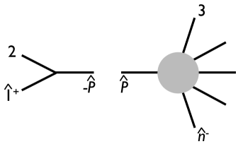
Figure 1: Two-particle factorization BCFW diagram. The hatted legs momenta are deformed following Eq. 4.

The terms in the BCFW recursion we are considering are those whose form is schematically illustrated in Fig. 1. We will refer to these as two-particle factorization channels, similar to what was used in [17]. This diagram can be expressed as

$$D_{+}=A_{\rm L}(\hat{1}^{+},2,-\hat{P})\frac{1}{s_{12}}A_{\rm{R}}(\hat{P},3,\dotsc,\hat{n}^{-})\ ,$$ (13)

with the following momentum assignments:

$$\hat{1} = 1]\langle 1-{\langle 12\rangle\over\langle n2\rangle}1]\langle n={\langle n1\rangle\over\langle n2\rangle}1]\langle 2\ ,$$

$$\hat{n} = n]\langle n+{\langle 12\rangle\over\langle n2\rangle}1]\langle n={(n+1)2\rangle\langle n\over\langle n2\rangle}\ ,$$

$$\hat{P} = \hat{1}+2={(2+1)n\rangle\langle 2\over\langle 2n\rangle}\,=\,2^{\prime}\ .$$ (14)

Note that with these assignments, $A_{\rm{R}}$ corresponds to an $n-1$-particle amplitude with the momenta of particles $n$ and $2$ shifted according to the inverse soft deformation, Eq. 3. It now remains to be shown that

$$A_{\rm L}(\hat{1}^{+},2,-\hat{P})\frac{1}{s_{12}}$$ (15)

is the soft factor for particle 1. We will show this explicitly for either helicity assignment of particle 2 in gauge theory and use the result in gravity to define the soft factor.

4.1 Gauge Theory

From the two possible helicity assignments of particle 2, there are two nonzero amplitudes, $A_{\rm L}(\hat{1}^{+},2^{-},-\hat{P}^{+})$ and $A_{\rm L}(\hat{1}^{+},2^{+},-\hat{P}^{-})$, which evaluate to the same result when including the shifted momentum. In particular,

$$A_{\rm L}(\hat{1}^{+},2^{+},-\hat{P}^{-})={[\hat{1}2]^{3}\over[2({-\hat{P}})][({-\hat{P}})\hat{1}]}=-{[12]\langle 2n\rangle\over\langle 1n\rangle}\ .$$ (16)

Including the factor of $1/s_{12}$ gives exactly the soft factor for particle $1$:

$$A_{\rm L}(\hat{1}^{+},2,-\hat{P})\frac{1}{s_{12}}={\cal S}(n,1^{+},2)=\frac{\langle n2\rangle}{\langle n1\rangle\langle 12\rangle}\ .$$ (17)

Putting the pieces together, we have shown that two-particle factorized BCFW terms can be computed with the inverse-soft procedure. Precisely, in gauge theory,

$$A_{\rm L}(\hat{1}^{+},2,-\hat{P})\frac{1}{s_{12}}A_{\rm R}(\hat{P},3,\dotsc,\hat{n}^{-})={\cal S}(n,1^{+},2)A_{\rm R}(2^{\prime},3,\dotsc,n^{\prime})\ ,$$ (18)

where the hat and prime represent respectively the BCFW (Eq. 2) and inverse soft momentum deformations (Eq. 3). With the $P$ and $C$ invariance of pure Yang-Mills theories this result also holds for a negative helicity soft particle.

For MHV or $\overline{\rm MHV}$ amplitudes in gauge theory, there only exist two-particle factorization channels, so we can write down an explicit inverse-soft recursion relation for these amplitudes. Specializing to MHV, these amplitudes are functions purely of the angle-bracket spinors and so the momentum shifts of Eq. 3 do not explicitly appear. That is,

$$A_{\rm MHV}(1,\dotsc,n^{+})={\cal S}(n-1,n^{+},1)A_{\rm MHV}(1,\dotsc,n-1)\ ;$$ (19)

to construct an MHV amplitude with one more particle we need only multiply by the appropriate soft factor.

4.2 Gravity

Motivated by the relationship between inverse soft and BCFW in gauge theory, we now turn to considering gravity. We begin as in gauge theory by constructing terms in the BCFW recursion relation and then expressing them in inverse-soft language. Much of the analysis from gauge theory carries over as three-point gravity amplitudes are just the square of the corresponding gauge-theory amplitudes. In gravity, we have

$$M_{\rm L}(\hat{1}^{+},2^{+},-\hat{P}^{-})={[\hat{1}2]^{6}\over[2({-\hat{P}})]^{2}[({-\hat{P}})\hat{1}]^{2}}={[12]^{2}\langle 2n\rangle^{2}\over\langle 1n\rangle^{2}}\ ,$$ (20)

where now the helicity labels mean helicity $\pm 2$. Including the propagator factor as in the gauge theory case gives

$$M_{\rm L}(\hat{1}^{+},2,-\hat{P})\frac{1}{s_{12}}=\frac{\langle n2\rangle^{2}[21]}{\langle n1\rangle^{2}\langle 12\rangle}\equiv{\cal G}(n,1^{+},2)\ .$$ (21)

We will take this as our definition of the gravity soft factor: an individual term in the sum in Eq. 8. To connect with that equation, note that the soft factor here is the $i=2$ term from Eq. 8 with reference momenta $q,r$ of graviton $1$’s polarization tensor set equal to the momentum of graviton $n$. Note that in contrast to the gauge-theory soft factor of Eq. 17, Eq. 21 is not (anti-)symmetric under the exchange of particles $2$ and $n$. Particle $n$’s momentum is the reference momentum whereas particle $2$ defines the adjacent particle or a term in the sum of Eq. 8. To reproduce the complete soft limit of particle 1 we must sum over terms of the form of Eq. 21, replacing $2$ successively by each particle in the amplitude. We will discuss in the next section how multiparticle factorization channels are produced with this soft factor.

As in gauge theory, MHV gravity amplitudes are constructed by the BCFW recursion from purely two-particle factorizations. Unlike their gauge-theory counterparts, gravity MHV amplitudes have explicit dependence on both angle- and square-bracket spinors. Unfortunately, this means that a simple inverse-soft recursion relation such as the one that was written down for gauge-theory MHV amplitudes cannot be written down for gravity since the inverse-soft deformations will appear explicitly in the lower-point amplitude. In any case, the BCFW recursion relations imply the inverse-soft recursion relation for MHV gravity amplitudes:

$$M_{\rm MHV}(1,\dotsc,n^{+})=\sum_{i=1}^{n-2}{\cal G}(n-1,n^{+},i)M_{\rm MHV}(1,\dotsc,i^{\prime},\dotsc,(n-1)^{\prime})\ ,$$ (22)

where the primes on the right side indicate the inverse-soft momentum deformation.

Nguyen, et al., introduced in [14] a distinct inverse-soft construction of gravity MHV amplitudes. In constructing MHV amplitudes, they used

$$\sum_{i=2}^{n}{i_{\mu}i_{\nu}\epsilon^{\mu\nu}(i)\over s_{i1}}=\sum_{i=2}^{n-2}{\langle in\rangle\langle i(n-1)\rangle[i1]\over\langle 1n\rangle\langle 1(n-1)\rangle\langle 1i\rangle}$$ (23)

as the form of the soft factor which first appeared in [18]. Using this soft factor has the benefit of making a larger permutation symmetry manifest as well as leading to a convenient “tree formula” for amplitudes. This tree formula has been shown to reproduce a previously conjectured MHV-level result [15]. Motivated by this work, Hodges presented a new formula for MHV gravity amplitudes in [16]. In our language, Hodges’ formula for MHV amplitudes can be expressed as

$$M_{\rm MHV}(1,\dotsc,n^{+})=\sum_{i=3}^{n-1}\frac{[in]\langle 1i\rangle\langle 2i\rangle}{\langle ni\rangle\langle 1n\rangle\langle 2n\rangle}M_{\rm MHV}(1^{\prime},\dotsc,i^{\prime},\dotsc,(n-1))\ .$$ (24)

Note that this equation has one fewer term than our corresponding formula, Eq. 22. Indeed, these two expressions for MHV gravity amplitudes are related by momentum conservation and a Schouten identity.

While the soft factor used in [14, 16] leads to nice expressions for MHV level amplitudes, difficulties arise when continuing to NMHV. Factorization channels with particles $1$ and $2$ on the same side of the factorization have no simple way to be constructed in this formalism. As we will see, this is another motivation for using the BCFW-inspired soft factor

$$\sum_{i=2}^{n}{i_{\mu}i_{\nu}\epsilon^{\mu\nu}(i)\over s_{i1}}=\sum_{i=2}^{n-1}{\langle in\rangle^{2}[i1]\over\langle 1n\rangle^{2}\langle 1i\rangle}$$ (25)

from which three-particle factorization channels can be constructed. Of course, the two expressions of the soft factor are equal, but because we work term by term in the sum, the BCFW-inspired soft factor leads more directly to multiparticle factorization.

5 Reproducing NMHV Amplitudes

We will now discuss how to construct NMHV amplitudes using the inverse-soft procedure. Our goal is to express the amplitude as a sum of terms, each of which is a a string of products of deformed soft factors times a lower-point amplitude. Schematically we want

$$A_{\text{NMHV}}\sim\sum\,\,\Bigg{(}\prod_{i=1}^{m}{\cal S}^{\prime}(p_{i})\Bigg{)}A^{\prime}_{n-m}\,,$$ (26)

where the $p_{i}$ have been removed from $A_{n-m}$. The prime indicates that the amplitudes and soft factors are deformed to conserve momentum as particles are removed. We will use the BCFW decomposition to determine which terms to include in the sum so the problem is reduced to expressing all BCFW diagrams entering the amplitude in the form of Eq. 26.

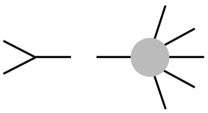
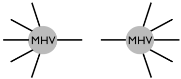
Figure 2: The two types of diagrams that enter the BCFW decomposition of an NMHV amplitude.

At NMHV level, there are two types of BCFW terms as illustrated in Fig. 2: those with a three-particle amplitude in the factorization and those with only higher-point MHV amplitudes. The former, illustrated in Fig. 2, was studied in the the previous section where it was expressed as a single soft factor times a deformed amplitude with one less particle. However, the diagram of Fig. 2 is new and we will now discuss how to express it in the form of Eq. 26. Note that $A_{\rm L}(\hat{1}^{+},2,\ldots,j,-\hat{P})$ is an on-shell MHV amplitude which can be expressed as a product of soft factors times a lower-point amplitude using Eqs. 19 or 22. One approach would then be to express $A_{\rm L}$ for gauge theory this way which would lead to the following expression for the full diagram:

$$D = A_{\rm L}(\hat{1}^{+},\ldots,-\hat{P})\,\frac{1}{P^{2}}\,A_{\rm R}(\hat{P},\ldots,\hat{n}^{-})$$ (27)

$$= {\cal S}(i,j^{+},k)\,A_{\rm L}(\hat{1}^{+},\ldots,i^{\prime},\overline{j},k^{\prime},\ldots,-\hat{P})\,\frac{1}{P^{2}}\,A_{\rm R}(\hat{P},\ldots,\hat{n}^{-})\,,$$

where particle $j$ has been removed from the amplitude in the second line. While Eq. 27 expresses the diagram as a product of a soft factor times lower-point amplitudes, an extra explicit propagator is present and there is more than one lower-point amplitude. Note also that $\hat{P}$ is the same in both lines of Eq. 27: it is the sum of all left-hand-side particles’ momenta including particle $j$. It is not an original particle whose momentum was deformed using inverse soft (compare with two-particle factorization in Eq. 4 where $\hat{P}$ is equal to $2^{\prime}$). Thus, Eq. 27 is not what we want and it does not express the diagram in the desired form of Eq. 26.

We will then adopt a different approach. We will build up $A_{\rm L}$ times the propagator starting with a three-point amplitude times a propagator factor,

$$D_{\text{start}}=A_{\rm L}(\hat{1}^{+},j,-\hat{P}){1\over s_{1j}}A_{\rm R}(\hat{P},j+1,\ldots,\hat{n}^{-})=S(n,1^{+},j)A_{\rm R}(j^{\prime},j+1,\ldots,n^{\prime-})$$ (28)

and will add particles until all that were contained in the original $A_{\rm L}$ are included. Namely, we will build the diagram of Fig. 2 starting with a two-particle diagram where only two particles are in the left-hand-side MHV amplitude. We add particles in turn to the left amplitude with soft factors and deforming the momenta appropriately. Thus, a three-particle factorization will have two soft factors, a four-particle factorization three and so on. We do not explicitly add particles to $A_{\rm R}$, but we must make sure that the momentum shifts generated by the work on the left correspond to the correct BCFW deformations. Thus, in order to achieve the form of Eq. 26, we have two requirements: $A_{\rm L}$ times the propagator must reduce to a product of soft factors and all inverse-soft shifted momenta must reproduce the BCFW-deformed momenta.

Unfortunately these requirements are not satisfied generically for any diagram of the form illustrated in Fig 2. For instance, we will see that particles’ momenta need to be deformed in a specific way and in a specific order to reproduce the BCFW shift. On the other hand, we need to keep $A_{\rm L}$ nonzero throughout the construction which can restrict which particle can be added at a given step. For instance, the nonzero three-point BCFW vertex with particle $\hat{1}^{+}$ has helicity $(+,+,-)$. Thus, the first particle to be added on the left must have negative helicity. Complications will also arise when trying to add a particle next to the unphysical momentum $\hat{P}$. These caveats will be discussed in detail in the next sections.

In section 5.1, we will discuss how the inverse-soft shift can reproduce the BCFW deformation in $A_{\rm R}$. In sections 5.2 and 5.3, we will see how $A_{\rm L}$ times the propagator can be constructed as a string of deformed soft factors separately for gauge theory and gravity. Finally, in section 5.4, we will summarize the above mentioned caveats and address the applicability of the procedure.

5.1 Momentum Deformation in $A_{\rm R}$

In this section we will show how the inverse-soft shift can be equivalent to the usual BCFW deformation in $A_{\rm R}$ at each step of the construction. We begin with a two-particle factorization diagram in Eq. 28 and the result from Eq. 4 that the associated deformation is equivalent to the BCFW shift. Here, we will write the deformed momentum differently from Eq. 4 to make the generalization to higher points easier:

$$j^{\prime} = 1+j+\frac{(1+j)^{2}}{\langle n(1+j)1]}\,1]\langle n\,=\,\hat{P}\,,$$

$$n^{\prime} = n+\frac{(1+j)^{2}}{\langle n(1+j)1]}\,1]\langle n\,=\,\hat{n}\,.$$ (29)

Now, let’s add particle $2$ deforming particles $1$ and $j$. Note that since the three-point vertex with $\hat{1}^{+}$ has helicity $(+,+,-)$, particle $2$ needs to have negative helicity. Thus, the $-$ helicity spinors are shifted and $|1]$ is not touched. This leads to $n^{\prime\prime}$ and $j^{\prime\prime}$:

$$j^{\prime\prime} = 1^{\prime}+j^{\prime}+\frac{(1^{\prime}+j^{\prime})^{2}}{\langle n(j^{\prime}+1^{\prime})1]}\,1]\langle n=1+2+j+\frac{(1+2+j)^{2}}{\langle n(1+2+j)1]}\,1]\langle n=\,\hat{P}\,,$$

$$n^{\prime\prime} = n+\frac{(1^{\prime}+j^{\prime})^{2}}{\langle n(1^{\prime}+j^{\prime})1]}\,1]\langle n=n+\frac{(1+2+j)^{2}}{\langle n(1+2+j)1]}\,1]\langle n\,=\,\hat{n}\,.$$ (30)

We can now add any number of positive helicity particles between particle $2$ and particle $j$. From Eq. 5.1, it is easy to see that the inverse-soft shifts on particles $2,\dotsc,j$ will continue to reproduce the correct BCFW deformation. Namely, at each step of the construction, the momentum assignments in $A_{\rm R}$ corresponds to the momentum assignments of a BCFW diagram with the particles currently present. It is interesting to note that inverse soft gives us a definite procedure to extract the $\hat{P}]$ and $\langle\hat{P}$ components of $\hat{P}$. Using the form of Eq. 4, we have:

$$j^{\prime\prime}={(j^{\prime}+1^{\prime})n\rangle\over\langle j^{\prime}n\rangle}\langle j^{\prime}=\frac{[1j](1+2+j)n\rangle}{\langle n(j+2)1]}\times\frac{[1(j+2)}{[1j]}=\hat{P}]\langle\hat{P}\ .$$ (31)

Finally, note that the particles on the left had to be deformed in a specific order to reproduce the BCFW shift. Namely, in going from the initial two-point diagram to a three-point diagram the two particles on the left need to be deformed (particles $1$ and $j$ in the example above). Afterward, the momentum of particle $1$ can no longer be touched. For instance, particles $2$ and $j$ would be shifted in Eq. 5.1 to add particle 3. Since which momenta get shifted is related to the position of the added particle, this will restrict which diagrams can be constructed. We will discuss this issue in more detail in section 5.4.

5.2 A Product of Soft Factors in Gauge Theory

We now turn to showing that $A_{\rm L}$ times the propagator can be constructed as a string of deformed soft factors. In gauge theory this can be achieved by starting with the three-point amplitude $A_{\rm L}(\hat{1}^{+},j,-\hat{P})$ and adding particles between $\hat{1}$ and $j$. This has the nice feature that no explicit $\hat{P}$ appears in the soft factors because particles are never added next to $\hat{P}$. However, note that

$$A_{\rm L}(\hat{1}^{+},j^{+},-\hat{P}^{+})=A_{\rm L}(\hat{1}^{+},j^{-},-\hat{P}^{-})=0,$$ (32)

where the second equality follows from the fact that $\langle\hat{P}|$ is proportional to $\langle j|$ as can be seen from Eq. 4. One consequence of Eq. 32 is that the initial nonzero three-point amplitude will necessarily be $\overline{\rm{MHV}}$ which is a function of square brackets. Momentum shifts coming from adding $+$ helicity particles will then be visible. Another more direct consequence is that if we are in the situation of Eq. 32, we will have to start with another three-point amplitude without particle $j$. The latter particle will need to be added through a soft factor which contains $\hat{P}$.

In the case where $A_{\rm L}(\hat{1}^{+},j,\hat{P})$ is nonzero we begin with the single soft factor

$$A(\hat{1}^{+},j,-\hat{P}){1\over s_{1j}}={\cal S}(n,1^{+},j),$$ (33)

particles can be added to it. First add the negative helicity particle, particle $2$ for definiteness, between $1$ and $j$ as

$$A(\hat{1}^{+},2^{-},j,-\hat{P}){1\over s_{12j}}={\cal S}(1,2^{-},j){\cal S}(n,1^{\prime+},j^{\prime})\ ,$$ (34)

where, in the second soft factor, we have to deform the momenta of particles $1$ and $j$ according to inverse soft. Note also that $s_{12j}=s_{1^{\prime}j^{\prime}}$. We can now add more positive helicity particles in the exact same way by inserting them one by one between particles $2$ and $j$.

Consider now the case where both $j$ and $\hat{P}$ have negative helicity. We will start with $A_{\rm L}(\hat{1}^{+},2^{+},-\hat{P}^{-})$ and add particle $j^{-}$ between $2$ and $\hat{P}$. We have

$$A_{\rm L}(\hat{1}^{+},2^{+},j^{-},-\hat{P}^{-})\frac{1}{s_{12j}}={\cal S}(2,j^{-},-\hat{P})A_{\rm L}(1^{+},2^{+},-\hat{P})\frac{1}{s_{12j}}\,,$$ (35)

where we used the usual formula, Eq. 19, to decompose the four-point $\overline{\text{MHV}}$ amplitude and both sides were multiplied by the propagator. Remember that because we are adding a negative helicity particle to a $\overline{\text{MHV}}$ amplitude, the shifts on $2$ and $\hat{P}$ are not visible in the three-point amplitude. The BCFW shift on particle $1$ also does not appear. We can then instead imagine shifting the angle spinors of particles $1$ and $2$ to make room for particle $j$. Then $1/s_{12j}=1/s_{1^{\prime}2^{\prime}}$. Also note that $P=1+2+j=1^{\prime}+2^{\prime}$. Thus, we can write

$$A_{\rm L}(\hat{1}^{+},2^{+},j^{-},-\hat{P}^{-})\frac{1}{s_{12j}} = {\cal S}(2,j^{-},\hat{P})A_{\rm L}(1^{\prime+},2^{\prime+},-\hat{P}^{-})\frac{1}{s_{1^{\prime}2^{\prime}}}$$ (36)

$$= {\cal S}(2,j^{-},\hat{P})\,{\cal S}(n,1^{\prime+},2^{\prime})$$

$$= {\cal S}(2,j^{-},2^{\prime\prime})\,{\cal S}(n,1^{\prime+},2^{\prime})\,,$$

where we used Eq. 17 to combine the soft factor with the propagator. In going from the second line to third line we have replaced $\hat{P}$ by $2^{\prime\prime}$ as in Eq. 31. Note also that the gauge-theory soft factor is symmetric in $\hat{P}\leftrightarrow-\hat{P}$.

It is insightful to do an explicit example. Inserting the soft-factor expressions into Eq. 36:

$${\cal S}(2,j^{-},2^{\prime\prime})\,{\cal S}(n,1^{\prime+},2^{\prime}) = \frac{[22^{\prime\prime}]}{[2j][j2^{\prime\prime}]}\,\frac{\langle n2^{\prime}\rangle}{\langle n1^{\prime}\rangle\langle 1^{\prime}2^{\prime}\rangle}$$ (37)

$$= \frac{[2(1+j)n\rangle}{[2j][j(1+2)n\rangle}\,\frac{\langle n(2+j)1][12]}{\langle n(1+j)2](1+2+j)^{2}}$$

$$= \frac{\langle n(2+j)1][12]}{[j(1+2)n\rangle[2j](1+2+j)^{2}}\,,$$

where we used the value of $2^{\prime\prime}]$ given in Eq. 31. We can now compare this with the expression obtained directly through BCFW,

$$A_{\rm L}(\hat{1}^{+},2^{+},j^{-},-\hat{P}^{-})\frac{1}{s_{12j}} = \frac{[12]^{3}}{[2j][j\hat{P}][\hat{P}1]}\,\frac{1}{s_{12j}}$$ (38)

$$= \frac{\langle n(2+j)1][12]}{[j(1+2)n\rangle[2j](1+2+j)^{2}}\,,$$

and it agrees with the inverse-soft construction as expected.

In summary, it is always possible to go from a two-particle to a three-particle diagram using inverse soft. The momenta of the two particles initially on the left are always deformed irrespective of the location of the added third particle. One can also see that it will not be possible to add particles next to $\hat{P}$ after this first step. Each time a particle is added adjacent to $\hat{P}$, the momentum of $1$ must be deformed to conserve momentum. In constructing a four-particle factorization channel we add a $+$ helicity particle which would induce a shift of $|1]$, destroying the equivalence of the BCFW and inverse soft shifts in $A_{\rm R}$; see Eq. 5.1. For the same reason, it is not possible to add a $+$ helicity particle next to particle $1$.

5.3 A Product of Soft Factors in Gravity

As there is no color ordering in gravity, soft particles must be inserted at all possible locations. This includes inserting the particle adjacent to the unphysical particle $\hat{P}$. As mentioned above, it is not possible to add next to $\hat{P}$ in a three-particle diagram to create a four-particle diagram. Consequently, in gravity, at most three-particle factorization diagrams can be created with inverse soft. Adding particle $2$ next to particles $j$ and $\hat{P}$ with particle $1$’s momentum the reference momentum (see Eq. 21), we find

$$M(\hat{1}^{+},2^{-},j,-\hat{P}){1\over s_{12j}} = \bigl{[}{\cal G}(1,2^{-},j)+{\cal G}(1,2^{-},-\hat{P})\bigr{]}{\cal G}(n,1^{\prime+},j^{\prime})$$

$$= \bigl{[}{\cal G}(1,2^{-},j)-{\cal G}(1,2^{-},j^{\prime\prime})\bigr{]}{\cal G}(n,1^{\prime+},j^{\prime})\ .$$

Note that the gravity soft factor is antisymmetric in $j^{\prime\prime}\leftrightarrow-j^{\prime\prime}$ which explains the minus sign in the second line of Eq. 5.3. To prove this, write the explicit values for the soft factors in the equation above:

$$\bigl{[}{\cal G}(1,2^{-},j)-{\cal G}(1,2^{-},j^{\prime\prime})\bigr{]}{\cal G}(n,1^{\prime+},j^{\prime}) = \Bigg{[}\frac{[j1]^{2}\langle 2j\rangle}{[21]^{2}[j2]}-\frac{[j^{\prime\prime}1]^{2}\langle 2j^{\prime\prime}\rangle}{[21]^{2}[j^{\prime\prime}2]}\Bigg{]}\frac{\langle nj^{\prime}\rangle^{2}[1j]}{\langle n1^{\prime}\rangle^{2}\langle j^{\prime}1^{\prime}\rangle}$$ (40)

$$= \frac{[1j]\langle j2\rangle\langle n(1+2)j]}{[21][j2]\langle n(j+1)2]}\times\frac{\langle n(j+2)1]^{2}[j1]^{2}}{\langle n(1+2)j]^{2}P^{2}}$$

$$= \frac{[1j]^{3}\langle j2\rangle\langle n(j+2)1]^{2}}{[21][j2]\langle n(j+1)2]\langle n(1+2)j]P^{2}}\,,$$

where we used the explicit value of $j^{\prime\prime}$ given in Eq. 31. For completeness, we will compute the left-hand side of Eq. 5.3 directly using the BCFW procedure:

$$M(\hat{1}^{+},2^{-},j,-\hat{P}){1\over s_{12j}} = -\frac{\langle 2j\rangle[\hat{P}1]^{6}}{[2j][2\hat{P}][21][j\hat{P}][j1]}\times\frac{1}{P^{2}}$$ (41)

$$= \frac{[1j]^{3}\langle j2\rangle\langle n(j+2)1]^{2}}{[21][j2]\langle n(j+1)2]\langle n(1+2)j]P^{2}}\,.$$

Thus, the expression built using inverse soft agrees with the usual BCFW construction as expected.

The requirement for a consistent inverse-soft construction, that such unphysical soft factors be included in constructing multiparticle gravity factorization channels, is very restrictive. The soft factor we have used to define the gravity inverse-soft factor is exactly what is needed to reproduce individual BCFW terms. As mentioned earlier, other soft factors, such as that from [14], could have significant difficulty in reproducing the multiparticle factorization channels precisely because of this issue.

5.4 Applicability of the procedure

In this section, we will summarize which diagrams and which NMHV helicity amplitudes can be constructed with the inverse-soft procedure discussed above. First, for gravity, we can construct all two- and three-particle factorization diagrams. However, as previously mentioned, four-particle diagrams cannot be created as they require adding a particle next to $\hat{P}$ in a three-particle diagram which destroys the BCFW deformation in $A_{\rm R}$. Thus, only NMHV gravity amplitudes with seven or fewer external particles ($n\leq 7$) can be constructed using inverse soft.

In gauge theory, we can also reproduce all two- and three-particle diagrams allowing us to construct all $n\leq 7$ amplitudes. However, we can do more as we can add particles between particles $2$ and $j$ to create four- and higher-point diagrams. Namely, we can create diagrams of the form

$$A_{\rm L}(\hat{1}^{+},2^{-},3^{+},\ldots,j^{\pm},-\hat{P}^{\mp})\frac{1}{P^{2}}A_{\rm R}(\hat{P}^{\pm},\ldots,\hat{n}^{-})\,,$$ (42)

$$A_{\rm L}(\hat{1}^{+},2^{+},3^{+},\ldots,j^{-},-\hat{P}^{-})\frac{1}{P^{2}}A_{\rm R}(\hat{P}^{+},\ldots,\hat{n}^{-})\,,$$ (43)

where in the first line we start with $A_{\rm L}(\hat{1}^{+},j^{\pm},-\hat{P}^{\mp})$, add particle $2^{-}$, and fill in with positive helicity particles between particles $2$ and $j$. In the second line, we start with $A_{\rm L}(\hat{1}^{+},2^{+},-\hat{P}^{-})$, add particle $j^{-}$ next to $\hat{P}$, and fill in again between $2$ and $j$.

Note that we can also take $A_{\rm L}$ as our lower point amplitude and add particles to $A_{\rm R}$. This will allow us to construct the additional diagrams

$$A_{\rm L}(\hat{1}^{+},\ldots,-\hat{P}^{+})\frac{1}{P^{2}}A_{\rm R}(\hat{P}^{-},(j+1)^{+},\ldots,(n-1)^{+},\hat{n}^{-})\,,$$ (44)

$$A_{\rm L}(\hat{1}^{+},\ldots,-\hat{P}^{-})\frac{1}{P^{2}}A_{\rm R}(\hat{P}^{+},(j+1)^{+},\ldots,(n-1)^{-},\hat{n}^{-})\,,$$ (45)

where in the first line we start with $A_{\rm R}(\hat{P}^{-},(n-1)^{+},n^{-})$, add particle $(j+1)^{+}$, and fill in with positive helicity particles between particles $(j+1)$ and $(n-1)$. In the second line, we start with $A_{\rm R}(\hat{P}^{+},(n-1)^{-},n^{-})$, add particle $(j+1)^{+}$ next to $\hat{P}$, and fill in again between $(j+1)$ and $(n-1)$.

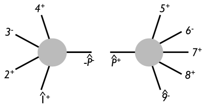
Figure 3: A BCFW diagram for the amplitude $A(1^{-},2^{+},3^{-},4^{+},5^{+},6^{-},7^{+},8^{+},9^{-})$ which cannot be constructed with inverse soft.

We now notice that any NMHV amplitude containing adjacent particles with helicity $(-,+,-)$ or $(-,-,+)$ can be created using the inverse-soft procedure we have developed here. In such a case, we factorize the amplitude in BCFW at the location of the $+$ helicity particle in this series: either $(-,\hat{+}|\hat{-})$ or $(-,\hat{-}|\hat{+})$. This factorization results in the possible constructible terms discussed above. Such a factorization is always possible in NMHV gauge-theory amplitudes up through eight external legs. Problems begin at nine points as illustrated in Fig. 3. The amplitude $A(1^{+},2^{+},3^{-},4^{+},5^{+},6^{-},7^{+},8^{+},9^{-})$ does not contain either of the strings of adjacent particles with helicity $(-,+,-)$ or $(-,-,+)$. The BCFW diagram in Fig. 3 would require adding two particles adjacent to $\hat{P}$ or adding a $+$ helicity particle next to particle $1$ and thus cannot be constructed using our inverse-soft procedure.

5.5 Example: Gauge Theory NMHV

To show the utility of inverse soft, we will give an explicit example of constructing the six-point NMHV gauge-theory amplitude using inverse soft. Consider the gauge-theory amplitude $A(1^{+},2^{-},3^{+},4^{-},5^{+},6^{-})$. We will deform the momenta of particles $3$ and $4$ for the BCFW construction. This deformation leads to three factorizations which contribute to the amplitude:

$$D_{1} = A(2^{-},\hat{3}^{+},-\hat{P})\frac{1}{s_{23}}A(\hat{P},\hat{4}^{-},5^{+},6^{-},1^{+})\ ,$$ (46)

$$D_{2} = A(1^{+},2^{-},\hat{3}^{+},-\hat{P})\frac{1}{s_{123}}A(\hat{P},\hat{4}^{-},5^{+},6^{-})\ ,$$

$$D_{3} = A(6^{-},1^{+},2^{-},\hat{3}^{+},-\hat{P})\frac{1}{s_{45}}A(\hat{P},\hat{4}^{-},5^{+})\ .$$

We will consider each of these terms in turn and show that they can be written simply in the inverse-soft construction language. For compactness, we will only decompose these diagrams down to soft factors times MHV or $\overline{\text{MHV}}$ amplitudes.

We first consider $D_{1}$. As shown earlier, for the choice of helicity of $P$ that gives a nonzero value, $A(2^{-},\hat{3}^{+},-\hat{P})(1/s_{23})={\cal S}(2,3^{+},4).$ Thus, we can equally express $D_{1}$ as

$$D_{1}={\cal S}(2,3^{+},4)A(2^{\prime-},1^{+},6^{-},5^{+},4^{\prime-})\ .$$ (47)

Note that the amplitude that remains is of $\overline{\text{MHV}}$-type and so the inverse soft momentum shift explicitly appears. The same arguments hold for $D_{3}$; this time, re-expressing the right side of the factorization. $D_{3}$ can be written as

$$D_{3}={\cal S}(3,4^{-},5)A(6^{-},1^{+},2^{-},3^{\prime+},5^{\prime+})\ .$$ (48)

$D_{2}$ is slightly more complicated and requires some care. We will rewrite the left side of the BCFW factorization as a product of two soft factors as in Eq. 34. To do this, we will start with the soft factor $S(1,3^{+},4)$ and add particle $2$ between $1$ and $3$. This gives

$$A(1^{+},2^{-},\hat{3}^{+},-\hat{P})\frac{1}{s_{123}}={[13]\over[12][23]}{\langle 1^{\prime}4\rangle\over\langle 1^{\prime}3^{\prime}\rangle\langle 3^{\prime}4\rangle}\equiv{\cal S}(1,2^{-},3){\cal S}(1^{\prime},3^{\prime+},4)\ ,$$ (49)

where the primes indicate the inverse soft momentum deformation with negative helicity particle $2$. The right side of the factorization is subtle but proceeds exactly as previously. We first add particle $3$ to the expression. This produces $A(1^{\prime+},6^{-},5^{+},4^{\prime-})$, where the primes indicate the inverse soft momentum deformation with particle $3$. Next, we add particle $2$ between particles $1$ and $3$. Thus, we now only deform the momentum of particles $1$ and $3$ by the momentum of $2$. To see how this affects the momentum of the particles in $A(1^{\prime+},6^{-},5^{+},4^{\prime-})$, consider first $1^{\prime}$. We have

$$1^{\prime}={(1+3)4\rangle\over\langle 14\rangle}\langle 1\ .$$ (50)

Deforming the momentum of $1$ and $3$ appropriately gives $1^{\prime\prime}$:

$$1^{\prime\prime}={(1+2+3)4\rangle[3(1+2)\over\langle 4(1+2)3]}\ .$$ (51)

As it must, this equals the momentum flowing through the BCFW cut, $\hat{P}=1+2+\hat{3}$. We can now consider the deformation of $4^{\prime}$. Starting with

$$4^{\prime}={(4+3)1\rangle\over\langle 41\rangle}\langle 4\ ,$$ (52)

$4^{\prime\prime}$ is then

$$4^{\prime\prime}=4]\langle 4+{(1+2+3)^{2}\over\langle 4(1+2)3]}3]\langle 4=\hat{4}\ .$$ (53)

Finally, we can express $D_{2}$ in inverse-soft language as

$$D_2=𝒮(1,2^{-},3)𝒮(1^{\prime },3^{\prime +},4)A(1^{\prime \prime +}$$

References

- [1] D. I. Olive, “Exploration of -Matrix Theory,” Phys. Rev. B135, 745-760 (1964); G. F. Chew, “The Analytic S-Matrix: A Basis for Nuclear Democracy”, W.A. Benjamin, Inc. (1966) 103p.; R. J. Eden, P. V. Landshoff, D. I. Olive, J. C. Polkinghorne, “The Analytic S-Matrix,” Cambridge University Press (1966) 287 p.
- [2] Z. Bern, L. J. Dixon, D. C. Dunbar, D. A. Kosower, “One loop n point gauge theory amplitudes, unitarity and collinear limits,” Nucl. Phys. B425, 217-260 (1994). [arXiv:hep-ph/9403226]; Z. Bern, L. J. Dixon, D. C. Dunbar, D. A. Kosower, “Fusing gauge theory tree amplitudes into loop amplitudes,” Nucl. Phys. B435, 59-101 (1995). [arXiv:hep-ph/9409265].
- [3] Z. Bern, L. J. Dixon, D. A. Kosower, “One loop amplitudes for e+ e- to four partons,” Nucl. Phys. B513, 3-86 (1998). [arXiv:hep-ph/9708239]; Z. Bern, V. Del Duca, L. J. Dixon, D. A. Kosower, “All non-maximally-helicity-violating one-loop seven-gluon amplitudes in N=4 super-yang-Mills theory,” Phys. Rev. D71, 045006 (2005). [arXiv:hep-th/0410224]; R. Britto, F. Cachazo, B. Feng, “Generalized unitarity and one-loop amplitudes in N=4 super-Yang-Mills,” Nucl. Phys. B725, 275-305 (2005). [arXiv:hep-th/0412103].
- [4] E. Witten, “Perturbative gauge theory as a string theory in twistor space,” Commun. Math. Phys. 252, 189-258 (2004). [arXiv:hep-th/0312171].
- [5] R. Britto, F. Cachazo, B. Feng, “New recursion relations for tree amplitudes of gluons,” Nucl. Phys. B715, 499-522 (2005). [arXiv:hep-th/0412308].
- [6] R. Britto, F. Cachazo, B. Feng, E. Witten, “Direct proof of tree-level recursion relation in Yang-Mills theory,” Phys. Rev. Lett. 94, 181602 (2005). [arXiv:hep-th/0501052].
- [7] J. M. Drummond, J. M. Henn, “All tree-level amplitudes in N=4 SYM,” JHEP 0904, 018 (2009). [arXiv:0808.2475].
- [8] F. A. Berends et al. [ CALKUL Collaboration ], “Multiple Bremsstrahlung in Gauge Theories at High-Energies. 4. The Process e+ e- gamma gamma gamma gamma,” Nucl. Phys. B239, 395 (1984).
- [9] N. Arkani-Hamed, F. Cachazo, C. Cheung, J. Kaplan, “A Duality For The S Matrix,” JHEP 1003, 020 (2010). [arXiv:0907.5418].
- [10] N. Arkani-Hamed, unpublished.
- [11] N. Arkani-Hamed, F. Cachazo, C. Cheung, J. Kaplan, unpublished.
- [12] F. Cachazo, D. Skinner, “On the structure of scattering amplitudes in N=4 super Yang-Mills and N=8 supergravity,” [arXiv:0801.4574]; F. Cachazo, “Sharpening The Leading Singularity,” [arXiv:0803.1988]; F. Cachazo, M. Spradlin, A. Volovich, “Leading Singularities of the Two-Loop Six-Particle MHV Amplitude,” Phys. Rev. D78, 105022 (2008). [arXiv:0805.4832].
- [13] M. Bullimore, “Inverse Soft Factors and Grassmannian Residues,” JHEP 1101, 055 (2011). [arXiv:1008.3110].
- [14] D. Nguyen, M. Spradlin, A. Volovich, C. Wen, “The Tree Formula for MHV Graviton Amplitudes,” JHEP 1007, 045 (2010). [arXiv:0907.2276].
- [15] Z. Bern, L. J. Dixon, M. Perelstein and J. S. Rozowsky, “Multileg one loop gravity amplitudes from gauge theory,” Nucl. Phys. B 546, 423 (1999) [arXiv:hep-th/9811140].
- [16] A. Hodges, “New expressions for gravitational scattering amplitudes,” [arXiv:1108.2227].
- [17] P. C. Schuster, N. Toro, “Constructing the Tree-Level Yang-Mills S-Matrix Using Complex Factorization,” JHEP 0906, 079 (2009). [arXiv:0811.3207].
- [18] F. A. Berends, W. T. Giele, H. Kuijf, “On relations between multi - gluon and multigraviton scattering,” Phys. Lett. B211, 91 (1988).
- [19] For reviews, see: L. J. Dixon, “Calculating scattering amplitudes efficiently,” [arXiv:hep-ph/9601359]; M. L. Mangano, S. J. Parke, “Multiparton amplitudes in gauge theories,” Phys. Rept. 200, 301-367 (1991). [arXiv:hep-th/0509223]; M. E. Peskin, “Simplifying Multi-Jet QCD Computation,” [arXiv:1101.2414];
- [20] S. Weinberg, “Photons and Gravitons in s Matrix Theory: Derivation of Charge Conservation and Equality of Gravitational and Inertial Mass,” Phys. Rev. 135, B1049-B1056 (1964).
- [21] J. Bedford, A. Brandhuber, B. J. Spence and G. Travaglini, “A recursion relation for gravity amplitudes,” Nucl. Phys. B 721, 98 (2005) [arXiv:hep-th/0502146]; F. Cachazo and P. Svrcek, “Tree level recursion relations in general relativity,” [arXiv:hep-th/0502160]; P. Benincasa, C. Boucher-Veronneau and F. Cachazo, “Taming tree amplitudes in general relativity,” JHEP 0711, 057 (2007) [arXiv:hep-th/0702032].
- [22] N. Arkani-Hamed and J. Kaplan, “On Tree Amplitudes in Gauge Theory and Gravity,” JHEP 0804, 076 (2008) [arXiv:0801.2385].
- [23] N. Arkani-Hamed, F. Cachazo, J. Kaplan, JHEP 1009, 016 (2010). [arXiv:0808.1446].
- [24] J. M. Drummond, J. Henn, G. P. Korchemsky, E. Sokatchev, “Dual superconformal symmetry of scattering amplitudes in N=4 super-Yang-Mills theory,” Nucl. Phys. B828, 317-374 (2010). [arXiv:0807.1095].
- [25] J. M. Drummond, J. M. Henn, J. Plefka, “Yangian symmetry of scattering amplitudes in N=4 super Yang-Mills theory,” JHEP 0905, 046 (2009). [arXiv:0902.2987].
- [26] E. Cremmer, B. Julia, “The SO(8) Supergravity,” Nucl. Phys. B159, 141 (1979).