THERMUS

Abstract

THERMUS is a package of C++ classes and functions allowing statistical-thermal model analyses of particle production in relativistic heavy-ion collisions to be performed within the ROOT framework of analysis. Calculations are possible within three statistical ensembles; a grand-canonical treatment of the conserved charges $B$, $S$ and $Q$, a fully canonical treatment of the conserved charges, and a mixed-canonical ensemble combining a canonical treatment of strangeness with a grand-canonical treatment of baryon number and electric charge. THERMUS allows for the assignment of decay chains and detector efficiencies specific to each particle yield, which enables sensible fitting of model parameters to experimental data.

PACS: 25.75.-q, 25.75.DW

, ,

PROGRAM SUMMARY

Manuscript Title: THERMUS - A Thermal Model Package for ROOT
Authors: S. Wheaton, J. Cleymans, M. Hauer
Program Title: THERMUS, version 2.1
Journal Reference:
Catalogue identifier:
Licensing provisions: none
Programming language: C++
Computer: PC, Pentium 4, 1 GB RAM (not hardware dependent)
Operating system: Linux: FEDORA, RedHat etc
RAM:
Keywords: statistical-thermal models, resonance decays, particle multiplicities, relativistic heavy-ion collisions
PACS: 25.75.-q, 25.75.DW
Classification: 17.7 Experimental Analysis - Fission, Fusion, Heavy-ion
External routines/libraries: ’Numerical Recipes in C’ [1], ROOT [2]

Nature of problem:

Statistical-thermal model analyses of heavy-ion collision data require the calculation of both primordial particle densities and contributions from resonance decay. A set of thermal parameters (the number depending on the particular model imposed) and a set of thermalised particles, with their decays specified, is required as input to these models. The output is then a complete set of primordial thermal quantities for each particle, together with the contributions to the final particle yields from resonance decay.

In many applications of statistical-thermal models it is required to fit experimental particle multiplicities or particle ratios. In such analyses, the input is a set of experimental yields and ratios, a set of particles comprising the assumed hadron resonance gas formed in the collision and the constraints to be placed on the system. The thermal model parameters consistent with the specified constraints leading to the best-fit to the experimental data are then output.

Solution method:

THERMUS is a package designed for incorporation into the ROOT [2] framework, used extensively by the heavy-ion community. As such, it utilises a great deal of ROOT’s functionality in its operation. Three distinct statistical ensembles are included in THERMUS, while additional options to include quantum statistics, resonance width and excluded volume corrections are also available.

THERMUS provides a default particle list including all mesons (up to the $K_{4}^{*}(2045)$) and baryons (up to the $\Omega^{-}$) listed in the July 2002 Particle Physics Booklet [3]. For each typically unstable particle in this list, THERMUS includes a text-file listing its decays. With thermal parameters specified, THERMUS calculates primordial thermal densities either by performing numerical integrations or else, in the case of the Boltzmann approximation without resonance width in the grand-canonical ensemble, by evaluating Bessel functions. Particle decay chains are then used to evaluate experimental observables (i.e. particle yields following resonance decay). Additional detector efficiency factors allow fine-tuning of the model predictions to a specific detector arrangement.

When parameters are required to be constrained, use is made of the ‘Numerical Recipes in C’ [1] function which applies the Broyden globally convergent secant method of solving nonlinear systems of equations. THERMUS provides the means of imposing a large number of constraints on the chosen model (amongst others, THERMUS can fix the baryon-to-charge ratio of the system, the strangeness density of the system and the primordial energy per hadron).

Fits to experimental data are accomplished in THERMUS by using the ROOT TMinuit class. In its default operation, the standard $\chi^{2}$ function is minimised, yielding the set of best-fit thermal parameters. THERMUS allows the assignment of separate decay chains to each experimental input. In this way, the model is able to match the specific feed-down corrections of a particular data set.

Running time: Depending on the analysis required, run-times vary from seconds (for the evaluation of particle multiplicities given a set of parameters) to several minutes (for fits to experimental data subject to constraints).

References:

• W. H. Press, S. A. Teukolsky, W. T. Vetterling, B. P. Flannery, Numerical Recipes in C: The Art of Scientific Computing (Cambridge University Press, Cambridge, 2002).

• R. Brun and F. Rademakers, Nucl. Inst. & Meth. in Phys. Res. A 389 (1997) 81.
  See also http://root.cern.ch/.

• K. Hagiwara et al., Phys. Rev. D 66 (2002) 010001.

1 Introduction

The statistical-thermal model has proved extremely successful [1, 2, 3] in describing the hadron multiplicities observed in relativistic collisions of both heavy-ions and elementary particles. The methods used in calculating these yields have been extensively reviewed in recent years [4, 5]. The success of these models has led to the creation of several software codes [6, 7, 8] that use experimental particle yields as input and calculate the corresponding chemical freeze-out temperature ($T$) and baryon chemical potential ($\mu_{B}$). In this paper we present THERMUS, a package of C++ classes and functions, which is based on the object-oriented ROOT framework [9]. All THERMUS C++ classes inherit from the ROOT base class TObject. This allows them to be fully integrated into the interactive ROOT environment, allowing all of the ROOT functionality in a statistical-thermal model analysis. Recent applications of THERMUS include [2, 10, 11, 12, 13, 14, 15, 16, 17, 18, 19]. An on-going effort to extend the range of applications of THERMUS has led to several publications on fluctuations in statistical models [20, 21, 22].

The paper is structured in the following way. In Section 2 an overview is presented of the theoretical model on which THERMUS is based. Section 3 outlines the structure and functionality of the THERMUS code, while Section 4 explains the installation procedure.

2 Overview of the Statistical-Thermal Model of Heavy-Ion Collisions

2.1 Choice of Ensemble

Within the statistical-thermal model there is a freedom regarding the ensemble with which to treat the quantum numbers $B$ (baryon number), $S$ (strangeness) and $Q$ (charge), which are conserved in strong interactions. The introduction of chemical potentials for each of these quantum numbers (i.e. a grand-canonical description) allows fluctuations about conserved averages. This is a reasonable approximation only when the number of particles carrying the quantum number concerned is large. In applications of the thermal model to high-energy elementary collisions, such as $pp$, $p\bar{p}$ and $e^{+}e^{-}$ collisions [23, 24], a canonical treatment of each of the quantum numbers is required. Within such a canonical description, quantum numbers are conserved exactly. In small systems or at low temperatures (more specifically, low $VT^{3}$ values), a canonical treatment leads to a suppression of hadrons carrying non-zero quantum numbers, since these particles have to be created in pairs. In heavy-ion collisions, the large number of baryons and charged particles generally allows baryon number and charge to be treated grand-canonically. However, at the low temperatures of the GSI SIS, the resulting low production of strange particles requires a canonical treatment of strangeness [25]. This is the so-called mixed-canonical approach.

In order to calculate the thermal properties of a system, one starts with an evaluation of its partition function. The form of the partition function obviously depends on the choice of ensemble. In the following sections, we consider the three ensembles most widely used in applications of the statistical-thermal model.

2.1.1 The Grand-Canonical Ensemble

This ensemble is the most widely used in applications to heavy-ion collisions [5, 26, 27, 28, 29, 30, 31, 32, 33, 34, 35]. Within this ensemble, conservation laws for energy and quantum or particle numbers are enforced on average through the temperature and chemical potentials.

In the case of a multi-component hadron gas of volume $V$ and temperature $T$, the logarithm of the total partition function is given by,

$$\ln Z^{GC}(T,V,\{\mu_{i}\}) = \sum_{\mathrm{species}\;i}{g_{i}V\over\left(2\pi\right)^{3}}\int d^{3}p\ln\left(1\pm e^{-\beta\left(E_{i}-\mu_{i}\right)}\right)^{\pm 1},$$ (1)

where $g_{i}$ and $\mu_{i}$ are, respectively, the degeneracy and chemical potential of hadron species $i$, $\beta\equiv 1/T$, while $E_{i}=\sqrt{p^{2}+m_{i}^{2}}$, where $m_{i}$ is the particle mass. The plus sign refers to fermions and the minus sign to bosons.

Since in relativistic heavy-ion collisions it is not individual particle numbers that are conserved, but rather the quantum numbers $B$, $S$ and $Q$, the chemical potential for particle species $i$ is given by,

$$\mu_{i} = B_{i}\mu_{B}+S_{i}\mu_{S}+Q_{i}\mu_{Q},$$ (2)

where $B_{i}$, $S_{i}$ and $Q_{i}$ are the baryon number, strangeness and charge, respectively, of hadron species $i$, and $\mu_{B}$, $\mu_{S}$ and $\mu_{Q}$ are the corresponding chemical potentials for these conserved quantum numbers.

Once the partition function is known, the particle multiplicities, entropy and pressure are obtained by differentiation:

$$N_{i}^{GC} = T{\partial\ln Z^{GC}\over\partial\mu_{i}},$$ (3)

$$S^{GC} = {\partial\over\partial T}\left(T\ln Z^{GC}\right),$$ (4)

$$P^{GC} = T{\partial\ln Z^{GC}\over\partial V}.$$ (5)

Furthermore, the energy is given by,

$$E^{GC} = T^{2}\frac{\partial\ln Z^{GC}}{\partial T}+\sum_{\mathrm{species}\;i}\mu_{i}\;N_{i}^{GC}.$$ (6)

Using the prescription for the particle multiplicity,

$$N_{i}^{GC} = {g_{i}V\over 2\pi^{2}}\sum_{k=1}^{\infty}(\mp 1)^{k+1}{m_{i}^{2}T\over k}K_{2}\left(km_{i}\over T\right)e^{\beta k\mu_{i}}=\sum_{k=1}^{\infty}z_{i}^{k}e^{\beta k\mu_{i}},$$ (7)

where we have introduced the $z_{i}^{k}$. Similar expressions exist for the energy, entropy and pressure.

In practice, the Boltzmann approximation (i.e. retaining just the $k=1$ term in Equation (7)) is reasonable for all particles except the pions. In this approximation,

$$\ln Z^{GC}\left(T,V,\{\mu_{i}\}\right) = \sum_{\mathrm{species}\;i}\frac{g_{i}V}{\left(2\pi\right)^{3}}\int d^{3}p\;e^{-\beta\left(E_{i}-\mu_{i}\right)}=\sum_{\mathrm{species}\;i}z_{i}^{1}\;e^{\beta\mu_{i}},$$ (8)

where $z_{i}^{1}$ is the single-particle partition function of hadron species $i$. Furthermore, under this approximation, $P=\sum_{\mathrm{species}\;i}N_{i}^{GC}T/V$ both for massive and massless particles, which is certainly not true for quantum statistics.

Since the use of quantum statistics requires numerical integration (or evaluation of infinite sums), while Boltzmann statistics can be implemented analytically, it is worthwhile to identify those regions in which quantum statistics deviate greatly from Boltzmann statistics. In most applications of the statistical-thermal model, only a small region of the $\mu-T$ parameter space is of interest. Using the freeze-out condition of constant $E/N$ [36], the thermal parameters, and hence the percentage deviation from Boltzmann statistics, can be determined as a function of the collision energy $\sqrt{s}$. From such an analysis it is evident that, for pions, quantum statistics must be implemented at all but the lowest energies (deviation at the level of 10%), while, for kaons, the deviation peaks at between 1 and 2%. For all other mesons, the deviation is below the 1% level. For baryons, the deviation is extremely small for all except the protons at small $\sqrt{s}$.

When quantum statistics are applied, restrictions have to be imposed on the chemical potentials so as to avoid Bose-Einstein condensation. The Bose-Einstein distribution function diverges if,

$$e^{\beta\left(m_{i}-\mu_{i}\right)}\leq 1.$$ (9)

Such Bose-Einstein condensation is avoided, provided that the chemical potentials of all bosons included in the resonance gas are less than their masses (i.e. $\mu_{i}<m_{i}$).

2.1.2 The Canonical Ensemble

Within this ensemble, quantum number conservation is exactly enforced. Considering the fully canonical treatment of $B$, $S$ and $Q$ in the Boltzmann approximation, as investigated in [37], the partition function for the system is given by,

$$Z_{B,S,Q} = {Z_{0}\over(2\pi)^{2}}\int_{-\pi}^{\pi}d\phi_{S}\;\int_{-\pi}^{\pi}d\phi_{Q}\;\cos\left(S\phi_{S}+Q\phi_{Q}-B\arg\omega\right)$$ (10)

$$\times\exp\left[2\sum_{\mathrm{mesons}\;j}z_{j}^{1}\;\cos\left(S_{j}\phi_{S}+Q_{j}\phi_{Q}\right)\right]I_{B}\left(2|\omega|\right),$$

where,

$$\omega \equiv \sum_{\mathrm{baryons}\;j}z_{j}^{1}\;e^{i(S_{j}\phi_{S}+Q_{j}\phi_{Q})},$$

$$z_{j}^{1} \equiv {g_{j}V\over\left(2\pi\right)^{3}}\int d^{3}p\;e^{-\beta E_{j}},$$

$Z_{0}$ represents the contribution of those hadrons with no net charges, and the sums over mesons and baryons extend only over the particles (i.e. not the anti-particles).

Once the partition function is known, we can calculate all thermodynamic properties of the system. Using thermodynamic relations it follows that,

$$S = {\partial\over\partial T}\left(T\ln Z_{B,S,Q}\right),$$ (11)

and,

$$P = T{\partial\ln Z_{B,S,Q}\over\partial V}.$$ (12)

Furthermore, the multiplicity of hadron species $i$ within this ensemble, $N_{i}^{B,S,Q}$, is calculated by multiplying the single-particle partition function for particle $i$, appearing in the canonical partition function, by a fictitious fugacity $\lambda_{i}$, differentiating with respect to $\lambda_{i}$, and then setting $\lambda_{i}$ to 1:

$$N_{i}^{B,S,Q} = \left.{\partial\ln Z_{B,S,Q}({\lambda_{i}})\over\partial\lambda_{i}}\right|_{\lambda_{i}=1}.$$ (13)

Following these prescriptions,

$$N_{i}^{B,S,Q} = \left({Z_{B-B_{i},S-S_{i},Q-Q_{i}}\over Z_{B,S,Q}}\right)\left.N_{i}^{GC}\right|_{\mu_{i}=0},$$ (14)

$$S^{B,S,Q} = \ln Z_{B,S,Q}+\sum_{\mathrm{species}\;i}\left({Z_{B-B_{i},S-S_{i},Q-Q_{i}}\over Z_{B,S,Q}}\right){\left.E_{i}^{GC}\right|_{\mu_{i}=0}\over T},$$ (15)

$$P^{B,S,Q} = \sum_{\mathrm{species}\;i}\left({Z_{B-B_{i},S-S_{i},Q-Q_{i}}\over Z_{B,S,Q}}\right)\left.P_{i}^{GC}\right|_{\mu_{i}=0},$$ (16)

$$E^{B,S,Q} = \sum_{\mathrm{species}\;i}\left({Z_{B-B_{i},S-S_{i},Q-Q_{i}}\over Z_{B,S,Q}}\right)\left.E_{i}^{GC}\right|_{\mu_{i}=0}.$$ (17)

One notices that, in the Boltzmann approximation, the particle and energy density and pressure of particle species $i$, within the canonical ensemble, differ from that in the grand-canonical formalism, with all chemical potentials set to zero, by a multiplicative factor $\left({Z_{B-B_{i},S-S_{i},Q-Q_{i}}/Z_{B,S,Q}}\right)$. This correction factor depends only on the thermal parameters of the system and the quantum numbers of the particle (i.e. the correction for the $\Delta^{+}$ and $p$ are the same). The entropy is, however, slightly different; the total entropy cannot be split into the sum of contributions from separate particles.

Now,

$$\lim_{V\rightarrow\infty}\left({Z_{B-B_{i},S-S_{i},Q-Q_{i}}\over Z_{B,S,Q}}\right)=e^{B_{i}\mu_{B}/T}e^{S_{i}\mu_{S}/T}e^{Q_{i}\mu_{Q}/T}.$$ (18)

Thus, for large systems, the grand-canonical results for the particle number, entropy, pressure and energy are approached [37].

2.1.3 The Mixed-Canonical (Strangeness-Canonical) Ensemble

Within this ensemble, the strangeness in the system is fixed exactly by its initial value of $S$, while the baryon and charge content are treated grand-canonically. For a Boltzmann hadron gas of strangeness $S$,

$$Z_{S} = {1\over 2\pi}\int_{-\pi}^{\pi}d\phi_{S}\;e^{-iS\phi_{S}}$$ (19)

$$\times\exp\left[\sum_{\mathrm{hadrons}\;i}{g_{i}V\over\left(2\pi\right)^{3}}\int d^{3}p\;e^{-\beta\left(E_{i}-\mu_{i}\right)}\;e^{iS_{i}\phi_{S}}\right],$$

where the sum over hadrons includes both particles and anti-particles and,

$$\mu_{i} = B_{i}\mu_{B}+Q_{i}\mu_{Q}.$$ (20)

Applying the same prescription for the evaluation of the particle multiplicities as discussed for the canonical ensemble, it follows that,

$$N_{i}^{S} = \left({Z_{S-S_{i}}\over Z_{S}}\right)\left.N_{i}^{GC}\right|_{\mu_{S}=0}.$$ (21)

Furthermore,

$$S^{S} = \ln Z_{S}+\sum_{\mathrm{species}\;i}\left({Z_{S-S_{i}}\over Z_{S}}\right)\left({\left.E_{i}^{GC}\right|_{\mu_{S}=0}-\mu_{i}\left.N_{i}^{GC}\right|_{\mu_{S}=0}\over T}\right),$$ (22)

$$P^{S} = \sum_{\mathrm{species}\;i}\left({Z_{S-S_{i}}\over Z_{S}}\right)\left.P_{i}^{GC}\right|_{\mu_{S}=0},$$ (23)

$$E^{S} = \sum_{\mathrm{species}\;i}\left({Z_{S-S_{i}}\over Z_{S}}\right)\left.E_{i}^{GC}\right|_{\mu_{S}=0}.$$ (24)

As in the case of the canonical ensemble, the strangeness-canonical results, in the Boltzmann approximation, differ from those of the grand-canonical ensemble, with $\mu_{S}=0$, by multiplicative correction factors which depend, in this case, only on the thermal parameters and the strangeness of the particle concerned. For large systems and high temperatures, these correction factors approach the grand-canonical fugacities, i.e.,

$$\lim_{V\rightarrow\infty}\left({Z_{S-S_{i}}\over Z_{S}}\right)=e^{S_{i}\mu_{S}/T}.$$ (25)

The expression for $Z_{S}$ can be reduced [38] to,

$$Z_{S}=Z_{0}\times\sum_{m=-\infty}^{+\infty}\sum_{n=-\infty}^{+\infty}I_{|3m+2n-S|}(x_{1}) \;I_{|n|}(x_{2})\;I_{|m|}(x_{3})$$

$$\times(y_{3}/y_{1}^{3})^{m}\;(y_{2}/y_{1}^{2})^{n}\;y_{1}^{S},$$

where $Z_{0}$ is the contribution to the total partition function of the non-strange hadrons, while,

$$x_{i} = 2\;\sqrt{k_{+i}k_{-i}}\hskip 28.45274pt(i=1,2,3),$$ (27)

and,

$$y_{i} = \sqrt{{k_{+i}\over k_{-i}}}\hskip 51.21504pt(i=1,2,3),$$ (28)

with,

$$k_{m}=\sum_{\mathrm{hadrons}\;j\;\mathrm{with}\;S_{j}=m}\left.n_{j}^{GC}\right|_{\mu_{S}=0}V.$$ (29)

In [39, 40] it is suggested that two volume parameters be used within canonical ensembles; the fireball volume at freeze-out, $V_{f}$, which provides the overall normalisation factor fixing the particle multiplicities from the corresponding densities, and the correlation volume, $V_{c}$, within which particles fulfill the requirement of local conservation of quantum numbers. In this way, by taking $V_{c}<V_{f}$, it is possible to boost the strangeness suppression. In fact, this was shown to be required to reproduce experimental heavy-ion collision data [39, 40].

2.2 Additional Features

2.2.1 Feeding from Unstable Particles

Since the particle yields measured by the detectors in collision experiments include feed-down from heavier hadrons and hadronic resonances, the primordial hadrons are allowed to decay to particles considered stable by the experiment before model predictions are compared with experimental data. For example, the total $\pi^{+}$ yield is given by,

$$N_{\pi^{+}}=\sum_{\mathrm{species}\;i}N_{i}^{(\mathrm{prim})}\>Br(i\rightarrow\pi^{+}),$$ (30)

where $Br(i\rightarrow\pi^{+})$ is the number of $\pi^{+}$’s into which a single particle of species $i$ decays. As shown in Figure 1, approximately 70% of $\pi^{+}$’s originate from resonance decay at RHIC energies. Thus, a full treatment of resonances is essential in any statistical-thermal analysis.

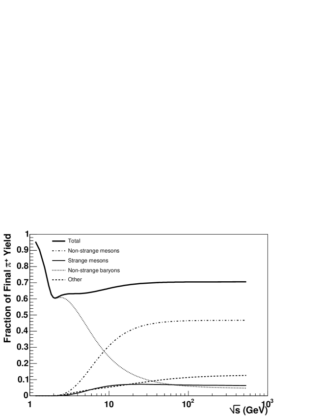
Figure 1: The energy dependence of the decay contribution to the final $\pi^{+}$ yield as predicted by the statistical-thermal model. Calculations performed within the grand-canonical formalism, assuming the constant $E/N$ freeze-out criterion [36] (weak decays excluded).

2.2.2 Resonances and the Inclusion of Resonance
Width

The inclusion of a mass cut-off in the measured resonance mass spectrum is motivated by the realisation that the time scale of a relativistic collision does not allow the heavier resonances to reach chemical equilibrium [41]. This assumes that inelastic collisions drive the system to chemical equilibrium. If the hadronisation process follows a statistical rule, then all resonances should, in principle, be included [31]. This is problematic, since data on the heavy resonances is sketchy. The situation is saved by the finite energy density of the system, resulting in a chemical freeze-out temperature at RHIC of approximately 160-170 MeV [42, 43], which strongly suppresses these heavy resonances and justifies their exclusion from the model. It is, however, important to check the sensitivity of the extracted thermal parameters to the chosen cut-off.

The finite width of the resonances is especially important at the low temperatures of the SIS. Resonance widths are included in the thermal model by distributing the resonance masses according to Breit-Wigner forms [23, 24, 27, 25, 41, 44]. This amounts to the following modification in the integration of the Boltzmann factor [25]:

$$\int d^{3}p\;\exp\left[-{\sqrt{p^{2}+m^{2}}\over T}\right]$$ (31)

$$\rightarrow\int d^{3}p\int ds\;\exp\left[-{\sqrt{p^{2}+s}\over T}\right]{1\over\pi}{m\Gamma\over(s-m^{2})^{2}+m^{2}\Gamma^{2}},$$

where $\Gamma$ is the width of the resonance concerned, with threshold limit $m_{\mathrm{threshold}}$ and mass $m$, and $\sqrt{s}$ is integrated over the interval [$m$ - $\delta m$, $m$ + $2\Gamma$], where $\delta m$ = min[$m$ - $m_{\mathrm{threshold}}$, $2\Gamma$].

2.2.3 Deviations from Equilibrium Levels

The statistical-thermal model applied to elementary $e^{+}e^{-}$, $pp$ and $p\bar{p}$ collisions [23, 24] indicates the need for an additional parameter, $\gamma_{S}$ (first introduced as a purely phenomenological parameter [45, 46]), to account for the observed deviation from chemical equilibrium in the strange sector. Since a canonical ensemble was considered in these analyses, there is an additional strangeness suppression at work, on top of the canonical suppression. Although strangeness production is expected to be greatly increased in $AA$ collisions, due to the larger interaction region and increased hadron rescattering, a number of recent analyses [44, 47, 48, 49, 50, 51] have found such a factor necessary to accomplish a satisfactory description of data.

Allowance for possibly incomplete strangeness equilibration is made by multiplying the Boltzmann factors of each particle species in the partition function (or thermal distribution function $f_{i}(x,p)$) by $\gamma_{S}^{\left|S_{i}\right|}$, where $\left|S_{i}\right|$ is the number of valence strange quarks and anti-quarks in species $i$. The value $\gamma_{S}=1$ obviously corresponds to complete strangeness equilibration.

It has been suggested [52] that a similar parameter, $\gamma_{q}$, should be included in thermal analyses to allow for deviations from equilibrium levels in the non-strange sector. Furthermore, as collider energies increase, so does the need for the inclusion of charmed particles in the statistical-thermal model, with their occupation of phase-space possibly governed by an additional parameter, $\gamma_{C}$.

2.2.4 Excluded Volume Corrections (Grand-Canonical Ensemble)

At very high energies, the ideal gas assumption is inadequate. In fact, the total particle densities predicted by the thermal model, with parameters extracted from fits to experimental data, far exceed reasonable estimates and measurements based on yields and the system size inferred by pion interferometry [53]. It becomes necessary to take into account the Van der Waals–type excluded volume procedure [53, 54, 55]. At the same fixed $T$ and $\mu_{B}$, all thermodynamic functions of the hadron gas are smaller than in the ideal hadron gas, and strongly decrease with increasing excluded volume.

Van der Waals–type corrections are included by making the following substitution for the volume $V$ in the canonical (with respect to particle number) partition function,

$$V \rightarrow V-\sum_{\mathrm{hadrons}\;i}\nu_{i}N_{i},$$ (32)

where $N_{i}$ is the number of hadron species $i$, and $\nu_{i}=4\left(4/3\pi r_{i}^{3}\right)$ is its proper volume, with $r_{i}$ its hard-sphere radius. This then leads to the following transcendental equation for the pressure of the gas in the grand-canonical ensemble (assuming $h$ particle species):

$$P(T,\mu_{1},...,\mu_{h}) = \sum_{i=1}^{h}P_{i}^{ideal}(T,\tilde{\mu_{i}}),$$ (33)

with,

$$\tilde{\mu_{i}} = \mu_{i}-\nu_{i}P(T,\mu_{1},...,\mu_{h}).$$ (34)

The particle, entropy and energy densities are given by,

$$n_{i}(T,\mu_{1},...,\mu_{h}) = \frac{n_{i}^{ideal}(T,\tilde{\mu_{i}})}{1+\sum_{j}\nu_{j}n_{j}^{ideal}(T,\tilde{\mu_{j}})},$$ (35)

$$s(T,\mu_{1},...,\mu_{h}) = \frac{\sum_{i}s_{i}^{ideal}(T,\tilde{\mu_{i}})}{1+\sum_{j}\nu_{j}n_{j}^{ideal}(T,\tilde{\mu_{j}})},$$ (36)

and,

$$e(T,\mu_{1},...,\mu_{h}) = \frac{\sum_{i}e_{i}^{ideal}(T,\tilde{\mu_{i}})}{1+\sum_{j}\nu_{j}n_{j}^{ideal}(T,\tilde{\mu_{j}})},$$ (37)

respectively. One sees that two suppression factors enter. The first suppression is due to the shift in chemical potential $\mu_{i}\rightarrow\tilde{\mu_{i}}$. In the Boltzmann approximation, this leads to a suppression factor $e^{-\nu_{i}P/T}$ in all thermodynamic quantities. The second suppression is due to the $[1+\sum_{j}\nu_{j}n_{j}^{ideal}(T,\tilde{\mu_{j}})]^{-1}$ factor.

In ratios of particle numbers, although the denominator correction cancels out, the shift in chemical potentials leads to a change in the case of quantum statistics. In the Boltzmann case, even these corrections cancel out, provided that the same proper volume parameter $\nu$ is applied to all species.

3 The Structure of THERMUS

3.1 Introduction

The three distinct ensemble choices outlined in Sections 2.1.1-2.1.3 are implemented in THERMUS. As input to the various thermal model formalisms one needs first a set of particles to be considered thermalised. When combined with a set of thermal parameters, all primordial densities (i.e. number density as well as energy and entropy density and pressure) are calculable. Once the particle decays are known, sensible comparisons can be made with experimentally measured yields.

In THERMUS, the following units are used for the parameters:

Parameter	Unit
Temperature ($T$)	GeV
Chemical Potential ($\mu$)	GeV
Radius	fm

Quantities frequently output by THERMUS are in the following units:

Quantity	Unit
Number Densities ($n$)	$\mathrm{fm}^{-3}$
Energy Density ($e$)	$\mathrm{GeV.fm}^{-3}$
Entropy Density ($s$)	$\mathrm{fm}^{-3}$
Pressure ($P$)	$\mathrm{GeV.fm}^{-3}$
Volume ($V$)	$\mathrm{fm}^{3}$

In the subsections to follow, we explain the basic structure and functionality of THERMUS (shown diagrammatically in Figure 2) by introducing the major THERMUS classes in a bottom-up approach. We begin with a look at the TTMParticle object.

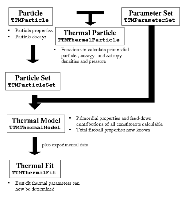
Figure 2: The basic structure of THERMUS (only the most fundamental base classes are shown).

3.2 The TTMParticle Class

The properties of a particle applicable to the statistical-thermal model are grouped in the basic TTMParticle object:

       ********* LISTING FOR PARTICLE Delta(1600)0 *********


                 ID = 32114

                 Deg. = 4

                 STAT = 1

                 Mass           =    1.6 GeV
                 Width          =   0.35 GeV
                 Threshold      = 1.07454 GeV

                 Hard sphere radius = 0

                 B = 1
                 S = 0                  |S| = 0
                 Q = 0
                 Charm = 0              |C| = 0
                 Beauty = 0
                 Top = 0

                 UNSTABLE

                 Decay Channels:


                 Summary of Decays:
         **********************************************

Besides the particle name, ‘Delta(1600)0’ in this case, its Monte Carlo numerical ID is also stored. This provides a far more convenient means of referencing the particle. The particle’s decay status is also noted. In this case, the $\Delta(1600)^{0}$ is considered unstable. Particle properties are input using the appropriate ‘setters’.

3.2.1 Inputting and Accessing Particle Decays

The TTMParticle class allows also for the storage of a particle’s decays. These can be entered from file. As an example, consider the decay file of the $\Delta(1600)^{0}$:

11.67   2112    111
5.83    2212    -211
29.33   2214    -211
3.67    2114    111
22.     1114    211
8.33    2112    113
4.17    2212    -213
15.     12112   111
7.5     12212   -211

Each line in the decay file corresponds to a decay channel. The first column lists the branching ratio of the channel, while the subsequent tab-separated integers represent the Monte Carlo ID’s of the daughters (each line (channel) can contain any number of daughters). The decay channel list of a TTMParticle object is populated with TTMDecayChannel objects by the SetDecayChannels function, with the decay file the first argument (only that part of the output that differs from the previous listing of the particle information is shown):

root [ ] part->SetDecayChannels("$THERMUS/particles/Delta\(1600\)0_decay.txt")
root [ ] part->List()

         ********* LISTING FOR PARTICLE Delta(1600)0 *********

                                     -
                                     -
                                     -


                 UNSTABLE

                 Decay Channels:
                 BRatio: 0.1167         Daughters:      2112    111
                 BRatio: 0.0583         Daughters:      2212    -211
                 BRatio: 0.2933         Daughters:      2214    -211
                 BRatio: 0.0367         Daughters:      2114    111
                 BRatio: 0.22           Daughters:      1114    211
                 BRatio: 0.0833         Daughters:      2112    113
                 BRatio: 0.0417         Daughters:      2212    -213
                 BRatio: 0.15           Daughters:      12112   111
                 BRatio: 0.075          Daughters:      12212   -211




                 Summary of Decays:
                2112            20%
                111             30.34%
                2212            10%
                -211            42.66%
                2214            29.33%
                2114            3.67%
                1114            22%
                211             22%
                113             8.33%
                -213            4.17%
                12112           15%
                12212           7.5%
         **********************************************

In many cases, the branching ratios of unstable hadrons do not sum to 100%. This can, however, be enforced by scaling all branching ratios. This is achieved when the second argument of SetDecayChannels is set to true (it is false by default).

In addition to the list of decay channels, a summary list of TTMDecay objects is generated in which each daughter appears only once, together with its total decay fraction. This summary list is automatically generated from the decay channel list when the SetDecayChannels function is called.

An existing TList can be set as the decay channel list of the particle, using the SetDecayChannels function. This function calls UpdateDecaySummary, thereby automatically ensuring consistency between the decay channel and decay summary lists.

The function SetDecayChannelEfficiency sets the reconstruction efficiency of the specified decay channel to the specified percentage. Again, a consistent decay summary list is generated.

Access to the TTMDecayChannel objects in the decay channel list is achieved through the GetDecayChannel method. If the extracted decay channel is subsequently altered, UpdateDecaySummary must be called to ensure consistency of the summary list.

3.3 The TTMParticleSet Class

The thermalised fireballs considered in statistical-thermal models typically contain approximately 350 different hadron and hadronic resonance species. To facilitate fast retrieval of particle properties, the TTMParticle objects of all constituents are stored in a hash table in a TTMParticleSet object. Other data members of this TTMParticleSet class include the filename used to instantiate the object and the number of particle species. Access to the entries in the hash table is through the particle Monte Carlo ID’s.

3.3.1 Instantiating a TTMParticleSet Object

In addition to the default constructor, the following constructors exist:

TTMParticleSet *set = new TTMParticleSet(char *file);

TTMParticleSet *set = new TTMParticleSet(TDatabasePDG *pdg);

The first constructor instantiates a TTMParticleSet object and inputs the particle properties contained in the specified text file. As an example of such a file, /$THERMUS/particles/PartList_PPB2002.txt contains a list of all mesons (up to the $K_{4}^{*}(2045)$) and baryons (up to the $\Omega^{-}$) listed in the July 2002 Particle Physics Booklet [56] (195 entries). Only particles need be included, since the anti-particle properties are directly related to those of the corresponding particle. The required file format is as follows:

0       Delta(1600)0    32114   4       +1      1.60000      0       1
0      0     0.35000    1.07454 (npi0)

• stability flag (1 for stable, 0 for unstable)

• particle name

• Monte Carlo particle ID (used for all referencing)

• spin degeneracy

• statistics (+1 for Fermi-Dirac, -1 for Bose-Einstein, 0 for Boltzmann)

• mass in GeV

• strangeness

• baryon number

• charge

• absolute strangeness content $\left|{S}\right|$

• width in GeV

• threshold in GeV

• string recording the decay channel from which the threshold is calculated if the particle’s width is non-zero

All further particle properties have to be set with the relevant ‘setters’ (e.g. the charm, absolute charm content and hard-sphere radius). By default, all properties not listed in the particle list file are assumed to be zero.

Figure 3 shows the distribution of resonances (both particle and anti-particle) derived from /$THERMUS/particles/PartList_PPB2002.txt. As collider energies increase, so does the need to include also the higher mass resonances. Although the TTMParticle class allows for the properties of charmed particles, these particles are not included in the default THERMUS particle list. If required, these particles have to be input by the user. The same applies to the hadrons composed of $b$ and $t$ quarks.

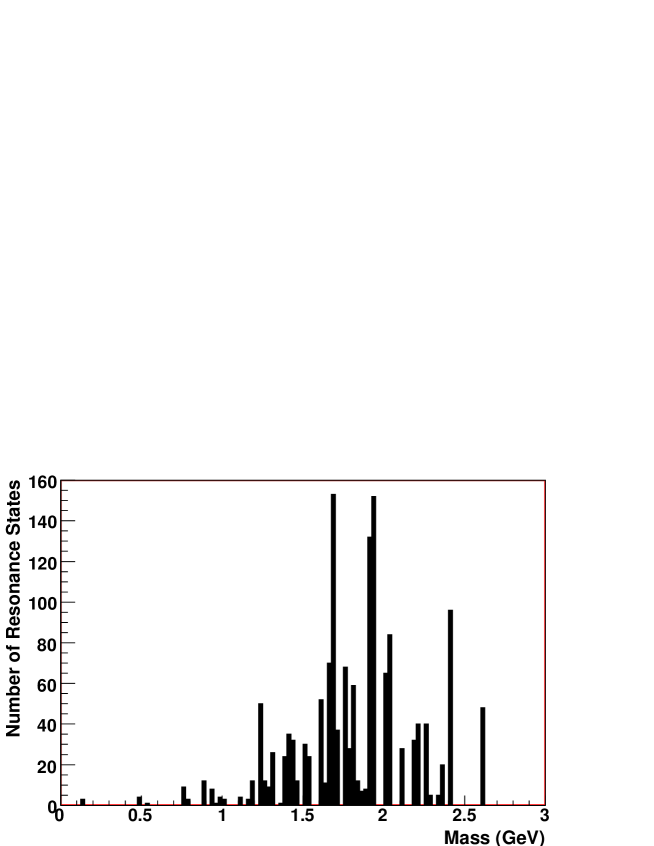
Figure 3: The mass distribution of the resonances included in PartList_PPB2002.txt.

It is also possible to use a TDatabasePDG object to instantiate a particle set. TDatabasePDG objects also read in particle information from text files. The default file is /$ROOTSYS/etc/pdg_table.txt and is based on the parameters used in PYTHIA [57].

The constructor TTMParticleSet(TDatabasePDG *pdg) extracts only those particles in the specified TDatabasePDG object in particle classes ‘Meson’, ‘CharmedMeson’, ‘HiddenCharmMeson’, ‘B-Meson’, ‘Baryon’, ‘CharmedBaryon’ and ‘B-Baryon’, as specified in /$ROOTSYS/etc/pdg_table.txt, and includes them in the hadron set. Anti-particles must be included in the TDatabasePDG object, as they are not automatically generated in this constructor of the TTMParticleSet class.

The default file read into the TDatabasePDG object, however, is incomplete; the charm, degeneracy, threshold, strangeness, $\left|S\right|$, beauty and topness of the particle are not included. Although the TDatabasePDG::ReadPDGTable function and default file allow for isospin, $I_{3}$, spin, flavor and tracking code to be entered too, the default file does not contain these values. Furthermore, all particles are made stable by default. Therefore, at present, using the TDatabasePDG class to instantiate a TTMParticleSet class should be avoided, at least until pdg_table.txt is improved.

3.3.2 Inputting Decays

Once a particle set has been defined, the decays to the stable particles in the set can be determined. After instantiating a TTMParticleSet object and settling on its stable constituents (the list of stable particles can be modified by adjusting the stability flags of the TTMParticle objects included in the TTMParticleSet object), decays can be input using the InputDecays method. Running this function populates the decay lists of all unstable particles in the set, using the decay files listed in the directory specified as the first argument. If a file is not found, then the corresponding particle is set to stable. For each typically unstable particle in /$THERMUS/particles/PartList_PPB2002.txt, there exists a file in /$THERMUS/particles listing its decays. The filename is derived from the particle’s name (e.g. Delta(1600)0_decay.txt for the $\Delta(1600)^{0}$). There are presently 195 such files, with entries based on the Particle Physics Booklet of July 2002 [56]. The decays of the corresponding anti-particles are automatically generated, while a private recursive function, GenerateBRatios, is invoked to ensure that only stable particles feature in the decay summary lists. The second argument of InputDecays, when set to true, scales the branching ratios so that their sum is 100%. As an example, consider the following (again only part of the listing is shown):

root [ ] TTMParticleSet set("$THERMUS/particles/PartList_PPB2002.txt")
root [ ] set.InputDecays("$THERMUS/particles/",true)
root [ ] TTMParticle *part = set.GetParticle(32114)
root [ ] part->List()

         ********* LISTING FOR PARTICLE Delta(1600)0 *********

                                     -
                                     -
                                     -

                 UNSTABLE

                 Decay Channels:
                 BRatio: 0.108558          Daughters:      2112    111
                 BRatio: 0.0542326         Daughters:      2212    -211
                 BRatio: 0.272837          Daughters:      2214    -211
                 BRatio: 0.0341395         Daughters:      2114    111
                 BRatio: 0.204651          Daughters:      1114    211
                 BRatio: 0.0774884         Daughters:      2112    113
                 BRatio: 0.0387907         Daughters:      2212    -213
                 BRatio: 0.139535          Daughters:      12112   111
                 BRatio: 0.0697674         Daughters:      12212   -211


                 Summary of Decays:
                2112            60.6774%
                111             62.5704%
                2212            39.3226%
                -211            83.9999%
                211             44.6773%
         **********************************************

For particle sets based on TDatabasePDG objects, decay lists should be populated through the function InputDecays(TDatabasePDG *). This function, however, does not automatically generate the anti-particle decays from those of the particle. Instead, the anti-particle decay list is used. Since the decay list may include electromagnetic and weak decays to particles other than the hadrons stored in the TTMParticleSet object, each channel is first checked to ensure that it contains only particles listed in the set. If not, the channel is excluded from the hadron’s decay list used by THERMUS. As mentioned earlier, care should be taken when using TDatabasePDG objects based on the default file, as it is incomplete.

An extremely useful function is ListParents(Int_t id), which lists all of the parents of the particle with the specified Monte Carlo ID. This function uses GetParents(TList *parents, Int_t id), which populates the list passed with the decays to particle id. Note that these parents are not necessarily ‘direct parents’; the decays may involve unstable intermediates.

3.3.3 Customising the Set

The AddParticle and RemoveParticle functions allow customisation of particle sets. Particle and anti-particle are treated symmetrically in the case of the former; if a particle is added, then its corresponding anti-particle is also added. This is not the case for the RemoveParticle function, however, where particle and anti-particle have to be removed separately.

Mass-cuts can be performed using MassCut(Double_t x) to exclude all hadrons with masses greater than the argument (expressed in GeV). Decays then have to be re-inserted, to remove the influence of the newly-excluded hadrons from the decay lists.

The function SetDecayEfficiency allows the reconstruction efficiency of the decays from a specified parent to the specified daughter to be set. Changes are reflected only in the decay summary list of the parent (i.e. not the decay channel list). Note that running UpdateDecaySummary or GenerateBRatios will remove any such changes, by creating again a summary list consistent with the channel list.

In addition to these operations, users can input their own particle sets by compiling their own particle lists and decay files.

3.4 The TTMParameter Class

This class groups all relevant information for parameters in the statistical-thermal model. Data members include:

fName	- the parameter name,
fValue	- the parameter value,
fError	- the parameter error,
fFlag	- a flag signalling the type of parameter (constrain, fit,
	fixed, or uninitialised),
fStatus	- a string reflecting the intended treatment or action taken.

In addition to these data members, the following, relevant to fit-type parameters, are also included:

fStart	- the starting value in a fit,
fMin	- the lower bound of the fit-range,
fMax	- the upper bound of the fit-range,
fStep	- the step-size.

The constructor and SetParameter(TString name, Double_t value, Double_t error) function set the parameter to fixed-type, by default. The parameter-type can be modified using the Constrain, Fit or Fix methods.

3.5 The TTMParameterSet Class

The TTMParameterSet class is the base class for all thermal parameter set classes. Each derived class contains its own TTMParameter array, with size determined by the requirements of the ensemble. The base class contains a pointer to the first element of this array. In addition, it stores the constraint information.

All derived classes contain the function GetRadius. In this way, TTMParameterSet is able to define a function, GetVolume, which returns the volume required to convert densities into total fireball quantities.

TTMParameterSetBSQ, TTMParameterSetBQ and TTMParameterSetCanBSQ are the derived classes.

3.5.1 TTMParameterSetBSQ

This derived class, applicable to the grand-canonical ensemble, contains the parameters:

$T$

$\mu_{B}$

$\mu_{S}$

$\mu_{Q}$

$\mu_{C}$

$\gamma_{S}$

$\gamma_{C}$

$R$,

where $R$ is the fireball radius, assuming a spherical fireball (i.e. $V=4/3\pi R^{3}$). In addition, the $B/2Q$ ratio and charm and strangeness density of the system are stored here. In the constructor, all errors are defaulted to zero, as is $R$, $\mu_{C}$, $S/V$, $C/V$ and $B/2Q$, while $\gamma_{C}$ is defaulted to unity.

Each parameter has a ‘getter’ (e.g. GetTPar), which returns a pointer to the requested TTMParameter object. In this class, $\mu_{S}$ and $\mu_{Q}$ can be set to constrain-type using ConstrainMuS and ConstrainMuQ, where the arguments are the required strangeness density and $B/2Q$ ratio, respectively. No such function exists for $\mu_{C}$, since constraining functions are not yet coded for the charm density. Each parameter of this class can be set to fit-type, using functions such as FitT (where the fit parameters have reasonable default values), or fixed-type, using functions such as FixMuB.

3.5.2 TTMParameterSetBQ

This derived class, applicable to the strangeness-canonical ensemble (strangeness exactly conserved and $B$ and $Q$ treated grand-canonically), has the parameters:

$T$

$\mu_{B}$

$\mu_{Q}$

$\gamma_{S}$

$R_{c}$

$R$,

where $R_{c}$ is the canonical or correlation radius; the radius inside which strangeness is exactly conserved. The fireball radius $R$, on the other hand, is used to convert densities into total fireball quantities. In addition, the required $B/2Q$ ratio is also stored, as well as the strangeness required inside the correlation volume (which must be an integer).

In addition to the same ‘getters’ and ‘setters’ as the previous derived class, it is possible to set $\mu_{Q}$ to constrain-type by specifying the $B/2Q$ ratio in the argument of ConstrainMuQ. The strangeness required inside the canonical volume is set through the SetS method. This value is defaulted to zero. The function ConserveSGlobally fixes the canonical radius, $R_{c}$, to the fireball radius, $R$. As in the case of the TTMParameterSetBSQ class, there also exist functions to set each parameter to fit or fixed-type.

3.5.3 TTMParameterSetCanBSQ

This set, applicable to the canonical ensemble with exact conservation of $B$, $S$ and $Q$, contains the parameters:

$T$

$B$

$S$

$Q$

$\gamma_{S}$

$R$.

Since all conservation is exact, there are no chemical potentials to satisfy constraints. Again, the same ‘getters’, ‘setters’ and functions to set each parameter to fit or fixed-type exist, as in the case of the previously discussed TTMParameterSet derived classes.

3.5.4 Example

As an example, let us define a TTMParameterSetBQ object. By default, all parameters are initially of fixed-type. Suppose we wish to fit $T$ and $\mu_{B}$, and use $\mu_{Q}$ to constrain the $B/2Q$ ratio in the model to that in Pb+Pb collisions:

root [ ] TTMParameterSetBQ parBQ(0.160,0.2,-0.01,0.8,6.,6.)
root [ ] parBQ.FitT(0.160)
root [ ] parBQ.FitMuB(0.2)
root [ ] parBQ.ConstrainMuQ(1.2683)
root [ ] parBQ.List()
  ***************************** Thermal Parameters ****************************

                 Strangeness inside Canonical Volume = 0

       T         =          0.16                    (to be FITTED)
                                                     start: 0.16
                                                     range: 0.05 -- 0.18
                                                     step:  0.001

     muB         =           0.2                    (to be FITTED)
                                                     start: 0.2
                                                     range: 0 -- 0.5
                                                     step:  0.001

     muQ         =         -0.01                    (to be CONSTRAINED)

                                                     B/2Q: 1.2683

  gammas         =           0.8                    (FIXED)

Can. radius      =             6                    (FIXED)

  radius         =             6                    (FIXED)

                         Parameters unconstrained

  ******************************************************************************

Note the default parameters for the $T$ and $\mu_{B}$ fits. Obviously, no constraining or fitting can take place yet; we have simply signalled our intent to take these actions at some later stage.

3.6 The TTMThermalParticle Class

By combining a TTMParticle and TTMParameterSet object, a thermal particle can be created. The TTMThermalParticle class is the base class from which thermal particle classes relevant to the three currently implemented thermal model formalisms, TTMThermalParticleBSQ, TTMThermalParticleBQ and TTMThermalParticleCanBSQ, are derived. Since no particle set is specified, the total fireball properties cannot be determined. Thus, in the grand-canonical approach, the constraints cannot yet be imposed to determine the values of the chemical potentials of constrain-type, while, in the strangeness-canonical and canonical formalisms, the canonical correction factors cannot yet be calculated. Instead, at this stage, the chemical potentials and/or correction factors must be specified.

Use is made of the fact that, in the Boltzmann approximation, $E/V$, $N/V$ and $P$, in the canonical and strangeness-canonical ensembles, are simply the grand-canonical values, with the chemical potential(s) corresponding to the canonically-treated quantum number(s) set to zero, multiplied by a particle-specific correction factor. This allows the functions for calculating $E/V$, $N/V$ and $P$ in the Boltzmann approximation to be included in the base class, which then also contains the correction factor as a data member (by definition, this correction factor is 1 in the grand-canonical ensemble).

Both functions including and excluding resonance width, $\Gamma$, are coded (e.g. DensityBoltzmannNoWidth and EnergyBoltzmannWidth). When width is included, a Breit-Wigner distribution is integrated over between the limits $[\mathrm{max}(m-2\Gamma,m_{\mathrm{threshold}}),m+2\Gamma]$.

3.6.1 TTMThermalParticleBSQ

This class is relevant to the grand-canonical treatment of $B$, $S$ and $Q$. In addition to the functions for calculating $E/V$, $N/V$ and $P$ in the Boltzmann approximation, defined in the base class, functions implementing quantum statistics for these quantities exist in this derived class (e.g. EnergyQStatNoWidth and PressureQStatWidth). Additional member functions of this class calculate the entropy using either Boltzmann or quantum statistics, with or without width.

In the functions calculating the thermal quantities assuming quantum statistics, it is first checked that the integrals converge for the bosons (i.e. there is no Bose-Einstein condensation). The check is performed by the ParametersAllowed method. A warning is issued if there are problems and zero is returned.

This class also accommodates charm, since the associated parameter set includes $\mu_{C}$ and $\gamma_{C}$, while the associated particle may have non-zero charm.

3.6.2 TTMThermalParticleBQ

This class is relevant to the strangeness-canonical ensemble. At present, this class is only applied in the Boltzmann approximation. Under this assumption, $N/V$, $E/V$ and $P$ are given by the grand-canonical result, with $\mu_{S}$ set to zero, up to a multiplicative correction factor. Since the total entropy does not split into the sum of particle entropies, no entropy calculation is made in this class.

3.6.3 TTMThermalParticleCanBSQ

This class is relevant to the fully canonical treatment of $B$, $S$ and $Q$. At present, as in the case of TTMThermalParticleBQ, this class is only applied in the Boltzmann approximation. Also, since the total entropy again does not split into the sum of particle entropies, no entropy calculation is made here.

3.6.4 Example

Let us construct a thermal particle, within the strangeness-canonical ensemble, from the $\Delta(1600)^{0}$ and the parameter set previously defined. Since this particle has zero strangeness, a correction factor of 1 is passed as the third argument of the constructor:

root [ ] TTMThermalParticleBQ therm_delta(part,&parBQ,1.)
root [ ] therm_delta.DensityBoltzmannNoWidth()
(Double_t)8.15072671710089913e-04
root [ ] therm_delta.EnergyBoltzmannWidth()
(Double_t)2.29185316377137748e-03

3.7 The TTMThermalModel Class

Once a parameter and particle set have been specified, these can be combined into a thermal model. TTMThermalModel is the base class from which the TTMThermalModelBSQ, TTMThermalModelBQ and TTMThermalModelCanBSQclasses are derived. A string descriptor is included as a data member of the base class to identify the type of model. This is used, for example, to handle the fact that the number of parameters in the associated parameter sets is different, depending on the model type.

All derived classes define functions to calculate the primordial particle, energy and entropy densities, as well as the pressure. These thermal quantities are stored in a hash table of TTMDensObj objects. Again, access is through the particle ID’s. In addition to the individual particles’ thermal quantities, the total primordial fireball strangeness, baryon, charge, charm, energy, entropy, and particle densities, pressure, and Wròblewski factor (see Section 3.7.11) are included as data members.

At this level, the constraints on any chemical potentials of constrain-type can be imposed, and the correction factors in canonical treatments can be determined. Also, as soon as the primordial particle densities are known, the decay contributions can be calculated.

3.7.1 Calculating Particle Densities

Running GenerateParticleDens clears the current entries in the density hash table of the TTMThermalModel object, automatically constrains the chemical potentials (where applicable), calculates the canonical correction factors (where applicable), and then populates the density hash table with a TTMDensObj object for each particle in the associated set. The decay contributions to each stable particle are also calculated, so that the density hash table contains both primordial and decay particle density contributions, provided of course that the decays have been entered in the associated TTMParticleSet object. In addition, the Wròblewski factor and total strangeness, baryon, charge, charm and particle densities in the fireball are calculated.

Note: The summary decay lists of the associated TTMParticleSet object are used to calculate the decay contributions. Hence, only stable particles have decay contributions reflected in the hash table. Unstable particles that are themselves fed by higher-lying resonances, do not receive a decay contribution.

Each derived class contains the private function PrimPartDens, which calculates only the primordial particle densities and, hence, the canonical correction factors, where applicable. In the case of the grand-canonical and strangeness-canonical ensembles, this function calculates the densities without automatically constraining the chemical potentials of constrain-type first. The constraining is handled by GenerateParticleDens, which calls external friend functions, which, in turn, call PrimPartDens. In the purely canonical ensemble, GenerateParticleDens simply calls PrimPartDens. In this way, there is uniformity between the derived classes. Since there is no constraining to be done, there is no real need for a separate function in the canonical case.

3.7.2 Calculating Energy and Entropy Densities and Pressure

GenerateEnergyDens, GenerateEntropyDens and GeneratePressure iterate through the existing density hash table and calculate and insert, respectively, the primordial energy density, entropy density and pressure of each particle in the set. In addition, they calculate the total primordial energy density, entropy density and pressure in the fireball, respectively. These functions require that the density hash table already be in existence. In other words, GenerateParticleDens must already have been run. If the parameters have subsequently changed, then this function must be run yet again to recalculate the correction factors or re-constrain the parameters, as required.

3.7.3 Bose-Einstein Condensation

When quantum statistics are taken into account (e.g. in TTMThermalModelBSQ or for the non-strange particles in TTMThermalModelBQ), certain choices of parameters lead to diverging integrals for the bosons (Bose-Einstein condensation). In these classes, a check, based on TTMThermalParticleBSQ::Parameters- Allowed, is included to ensure that the parameters do not lead to problems. Including also the possibility of incomplete strangeness and/or charm saturation (i.e. $\gamma_{S}\neq 1$ and/or $\gamma_{C}\neq 1$), Bose-Einstein condensation is avoided, provided that,

$$e^{\left(m_{i}-\mu_{i}\right)/T}>\gamma_{S}^{\left|S_{i}\right|}\gamma_{C}^{\left|C_{i}\right|},$$ (38)

for each boson. If this condition is failed to be met for any of the bosons in the set, a warning is issued and the densities are not calculated.

3.7.4 Accessing the Thermal Densities

The entries in the density hash table are accessed using the particle Monte Carlo ID’s. The function GetDensities(Int_t ID) returns the TTMDensObj object containing the thermal quantities of the particle with the specified ID. The primordial particle, energy, and entropy densities, pressure, and decay density are extracted from this object using the GetPrimDensity, GetPrimEnergy, GetPrimEntropy, GetPrimPressure, and GetDecayDensity functions of the TTMDensObj class, respectively. The sum of the primordial and decay particle densities is returned by TTMDensObj::GetFinalDensity. TTMDensObj::List outputs to screen all thermal densities stored in aTTMDensObj object.

ListStableDensities lists the densities (primordial and decay contributions) of all those particles considered stable in the particle set associated with the model. Access to the total fireball densities is through separate ‘getters’ defined in the TTMThermalModel base class (e.g. GetStrange, GetBaryon etc.).

3.7.5 Further Functions

GenerateDecayPartDens and GenerateDecayPartDens(Int_t id) (both defined in the base class) calculate decay contributions to stable particles. The former iterates through the density hash table and calculates the decay contributions to all those particles considered stable in the set. The latter calculates just the contribution to the stable particle with the specified ID. In both cases, the primordial densities must be calculated first. In fact, GenerateParticleDens automatically calls GenerateDecayPartDens, so that this function does not have to be run separately under ordinary circumstances. However, if one is interested in investigating the effect of decays, while keeping the parameters (and hence the primordial densities) fixed, then running these functions is best (the hash table will not be repeatedly cleared and repopulated with the same primordial densities).

ListDecayContributions(Int_t d_id) lists the contributions (in percentage and absolute terms) of decays to the daughter with the specified ID. The primordial and decay densities must already appear in the density hash table (i.e. run GenerateParticleDens first). ListDecayContribution(Int_t p_id, Int_t d_id) lists the contribution of the decay from the specified parent (with ID p_id) to the specified daughter (with ID d_id). The percentages listed by each of these functions are those of the individual decays to the total decay density.

Next we consider the specific features of the derived TTMThermalModel classes.

3.7.6 TTMThermalModelBSQ

In the grand-canonical ensemble, quantum statistics can be employed and, hence, there is a flag specifying whether to use Fermi-Dirac and Bose-Einstein statistics or Boltzmann statistics. The constructor, by default, includes both the effect of quantum statistics and resonance width. The flags controlling their inclusion are set using the SetQStats and SetWidth functions, respectively. The functions that calculate the particle, energy, and entropy densities, and pressure then use the corresponding functions in the TTMThermalParticleBSQ class to calculate these quantities in the required way. The statistics data member (fStat) of each TTMParticle included in the associated set can be used to fine-tune the inclusion of quantum statistics; with the quantum statistics flag switched on, Boltzmann statistics are still used for those particles with fStat=0.

In this ensemble, at this stage, both $\mu_{S}$ and $\mu_{Q}$ can be constrained (either separately or simultaneously). In order to accomplish this, the $\mu_{S}$ and/or $\mu_{Q}$ parameters in the associated TTMParameterSetBSQ object must be set to constrain-type.

It is also possible to constrain $\mu_{B}$ by the primordial ratio $E/N$ (the average energy per hadron), $n_{b}+n_{\bar{b}}$ (the total primordial baryon plus anti-baryon density), or $s/T^{3}$ (the primordial, temperature-normalised entropy density). This is accomplished by the ConstrainEoverN, ConstrainTotalBaryonDensity and ConstrainSoverT3 methods, respectively. Running these functions will adjust $\mu_{B}$ such that $E/N$, $n_{b}+n_{\bar{b}}$ or $s/T^{3}$, respectively, has the required value, regardless of the parameter type of $\mu_{B}$. In addition, the percolation model [58] can be imposed to constrain $\mu_{B}$ using ConstrainPercolation.

This class also accommodates charm, since the associated parameter set includes $\mu_{C}$ and $\gamma_{C}$, while the associated particle set may contain charmed particles. However, no constraining functions have yet been written for the charm content within this ensemble.

Within the grand-canonical ensemble, it is possible to include excluded volume effects. Their inclusion is controlled by the fExclVolCorrection flag, false by default, which is set through the SetExcludedVolume function. When included, these corrections are calculated on calling GenerateParticleDens, based on the hard-sphere radii stored in the TTMParticle objects of the associated particle set.

3.7.7 TTMThermalModelBQ

This class contains the following additional data members:

flnZtot	- log of the total partition function,
flnZ0	- log of the non-strange component of the partition function,
fExactMuS	- equivalent strangeness chemical potential,
fCorrP1	- canonical correction for S = +1 particles,
fCorrP2	- canonical correction for S = +2 particles,
fCorrP3	- canonical correction for S = +3 particles,
fCorrM1	- canonical correction for S = -1 particles,
fCorrM2	- canonical correction for S = -2 particles,
fCorrM3	- canonical correction for S = -3 particles.

Although this ensemble is only applied in the Boltzmann approximation for $S\neq 0$ hadrons, it is possible to apply quantum statistics to the $S=0$ hadrons. This is achieved through the SetNonStrangeQStats function. By default, quantum statistics is included for the non-strange hadrons by the constructors. Resonance width can be included for all hadrons, and is achieved through the SetWidth function. The constructors, by default, apply resonance width. The functions that calculate the particle, energy, and entropy densities, and pressure then use the corresponding functions in the TTMThermalParticle classes to calculate these quantities in the required way.

GenerateParticleDens populates the density hash table with particle densities, including the canonical correction factors, which are also stored in the appropriate data members. The equivalent strangeness chemical potential is calculated from the canonical correction factor for $S=+1$ particles. In the limit of large $VT^{3}$, this approaches the value of $\mu_{S}$ in the equivalent grand-canonical treatment.

Running GenerateEntropyDens populates each TTMDensObj object in the hash table with only that part of the total entropy that can be unambiguously attributed to that particular particle. There is a term in the total entropy that cannot be split; this is added to the total entropy at the end, but not included in the individual entropies (i.e. summing up the entropy contributions of each particle will not give the total entropy).

At this stage, in this formalism, $\mu_{Q}$ can be constrained (this is automatically realised if this parameter is set to constrain-type), while the correlation radius ($R_{c}$) can be set to the fireball radius ($R$) by applying the function ConserveSGlobally to the associated TTMParameterSetBQ object.

In exactly the same way as in the grand-canonical ensemble case, $\mu_{B}$ can be constrained in this ensemble by the primordial ratio $E/N$ (the average energy per hadron), $n_{b}+n_{\bar{b}}$ (the total primordial baryon plus anti-baryon density), or $s/T^{3}$ (the primordial, temperature-normalised entropy density), as well as by the percolation model.

3.7.8 TTMThermalModelCanBSQ

This class contains, amongst others, the following data members:

flnZtot	- log of the total canonical partition function,
fMuB,fMuS,fMuQ	- equivalent chemical potentials,
fCorrpip	- correction for $\pi^{+}$-like particles,
fCorrpim	- correction for $\pi^{-}$-like particles,
fCorrkm	- correction for $K^{-}$-like particles,
fCorrkp	- correction for $K^{+}$-like particles,
fCorrk0	- correction for $K^{0}$-like particles,
fCorrak0	- correction for $\bar{K}^{0}$-like particles,
fCorrproton	- correction for $p$-like particles,
fCorraproton	- correction for $\bar{p}$-like particles,
fCorrneutron	- correction for $n$-like particles,
fCorraneutron	- correction for $\bar{n}$-like particles,
fCorrlambda	- correction for $\Lambda$-like particles,
fCorralambda	- correction for $\bar{\Lambda}$-like particles,
fCorrsigmap	- correction for $\Sigma^{+}$-like particles,
fCorrasigmap	- correction for $\bar{\Sigma}^{-}$-like particles,
fCorrsigmam	- correction for $\Sigma^{-}$-like particles,
fCorrasigmam	- correction for $\bar{\Sigma}^{+}$-like particles,
fCorrdeltam	- correction for $\Delta^{-}$-like particles,

fCorradeltam	- correction for $\bar{\Delta}^{+}$-like particles,
fCorrdeltapp	- correction for $\Delta^{++}$-like particles,
fCorradeltapp	- correction for $\bar{\Delta}^{--}$-like particles,
fCorrksim	- correction for $\Xi^{-}$-like particles,
fCorraksim	- correction for $\bar{\Xi}^{+}$-like particles,
fCorrksi0	- correction for $\Xi^{0}$-like particles,
fCorraksi0	- correction for $\bar{\Xi}^{0}$-like particles,
fCorromega	- correction for $\Omega^{-}$-like particles,
fCorraomega	- correction for $\bar{\Omega}^{+}$-like particles.

Since this ensemble is only applied in the Boltzmann approximation, there is no flag for quantum statistics. However, resonance width can be included. This is achieved through the SetWidth function. The constructor, by default, applies resonance width. The functions that calculate the particle, energy, and entropy densities, and pressure then use the corresponding functions in the TTMThermalParticle classes to calculate these quantities in the required way.

GenerateParticleDens calls PrimPartDens, which calculates the particle densities, including the canonical correction factors, which are then also stored in the relevant data members accessible through the GetCorrFactor method. The integrands featuring in the evaluation of the partition function and correction factors can be viewed after calling PopulateZHistograms. This function populates the array passed as argument with histograms showing these integrands as a function of the integration variables $\phi_{S}$ and $\phi_{Q}$. Since these histograms are created off of the heap, they must be cleaned up afterwards.

GenerateEntropyDens acts in exactly the same way as in the strangeness-canonical ensemble case.

3.7.9 Example

As an example, we consider the strangeness-canonical ensemble, based on the particle set and strangeness-canonical parameter set previously defined. After instantiating the object, we populate the hash table with primordial and decay particle densities:

root [ ] TTMThermalModelBQ modBQ(&set,&parBQ)
root [ ] modBQ.GenerateParticleDens()
root [ ] parBQ.List()

  ***************************** Thermal Parameters ****************************

                 Strangeness inside Canonical Volume = 0

       T         =          0.16                    (to be FITTED)
                                                     start: 0.16
                                                     range: 0.05 -- 0.18
                                                     step:  0.001

     muB         =           0.2                    (to be FITTED)
                                                     start: 0.2
                                                     range: 0 -- 0.5
                                                     step:  0.001

     muQ         =       -0.00636409                (*CONSTRAINED*)

                                                     B/2Q: 1.2683

  gammas         =           0.8                    (FIXED)

Can. radius      =             6                    (FIXED)

  radius         =             6                    (FIXED)

                         B/2Q Successfully Constrained

  ******************************************************************************

One notices that the constraint on $\mu_{Q}$ is now automatically imposed.

The energy and entropy densities and pressure can be calculated once GenerateParticleDens has been run:

root [ ] modBQ.GenerateEnergyDens()
root [ ] modBQ.GenerateEntropyDens()
root [ ] modBQ.GeneratePressure()

Now, suppose that we are interested in the thermal densities of the $\Delta(1600)^{0}$ and $\pi^{+}$:

root [ ] TTMDensObj *delta_dens = modBQ.GetDensities(32114)
root [ ] delta_dens->List()
  **** Densities for Particle 32114 ****
         n_prim = 0.00138306
         n_decay = 0
         e_prim = 0.0022912
         s_prim = 0.0139745
         p_prim = 0.000221328

root [ ] TTMDensObj *piplus_dens = modBQ.GetDensities(211)
root [ ] piplus_dens->List()
  **** Densities for Particle 211 ****
         n_prim = 0.0488139
         n_decay = 0.119683
         e_prim = 0.0247039
         s_prim = 0.20276
         p_prim = 0.00742708

One notices that the $\pi^{+}$ has a decay density contribution, while the $\Delta(1600)^{0}$ does not. This is because, unlike the $\Delta(1600)^{0}$, the $\pi^{+}$ was considered stable.

3.7.10 Imposing of Constraints

The ‘Numerical Recipes in C’ [59] function applying the Broyden globally convergent secant method of solving nonlinear systems of equations is employed by THERMUS to constrain parameters. The input to the Broyden method is a vector of functions for which roots are sought. Typically, in the thermal model, solutions to the following equations are required (either separately or simultaneously):

$$\left({B/V\over 2Q/V}\right)_{primordial}^{model}-\left({B\over 2Q}\right)^{colliding\;system} = 0,$$

$$S_{primordial}^{model}-S^{colliding\;system} = 0,$$

$$\left({E/V\over N/V}\right)_{primordial}^{model}-\left(E\over N\right)^{required} = 0.$$

Although, as written, these equations are correct, the quantities $B/2Q$, $S$ and $E/N$ are typically of different orders of magnitude. Since the Broyden method in ‘Numerical Recipes in C’ defines just one tolerance level for function convergence (TOLF), it is important to ‘normalise’ each equation:

$$\left\{\left({B/V\over 2Q/V}\right)_{primordial}^{model}-\left({B\over 2Q}\right)^{colliding\;system}\right\}/\left({B\over 2Q}\right)^{colliding\;system} = 0,$$

$$\left\{S_{primordial}^{model}-S^{colliding\;system}\right\}/S^{colliding\;system} = 0,$$

$$\left\{\left({E/V\over N/V}\right)_{primordial}^{model}-\left({E\over N}\right)^{required}\right\}/\left({E\over N}\right)^{required} = 0.$$

This is the most democratic way of treating the constraints. However, this method obviously fails in the event of one of the denominators being zero. For the equations considered above, this is only likely in the case of the strangeness constraint, where the initial strangeness content is typically zero. In this case, where the strangeness carried by the positively strange particles $S_{+}$ is balanced by the strangeness carried by the negatively strange particles $S_{-}$, we write as our function to be satisfied,

$$\left(S/V\right)_{primordial}^{model}/\left(|S_{+}|_{primordial}^{model}/V+|S_{-}|_{primordial}^{model}/V\right) = 0.$$

In this way, the constraints can be satisfied to equal relative degrees, and equally well fractionally at each point in the parameter space. In addition to the constraints listed above, THERMUS also allows for the constraining of the total baryon plus anti-baryon density and the temperature-normalised entropy density, $s/T^{3}$, as well as the imposing of the percolation model.

3.7.11 Calculation of the Wròblewski Factor

The Wròblewski factor [60] is defined as,

$$\lambda_{S} = \frac{2<s\bar{s}>}{<u\bar{u}>+<d\bar{d}>},$$

where $<u\bar{u}>+<d\bar{d}>$ is the sum of newly-produced $u\bar{u}$ and $d\bar{d}$ pairs, while all $s\bar{s}$ pairs are newly-produced if $S=0$ in the initial state.

In THERMUS, $\lambda_{S}$ is calculated in the following way:

• Using the primordial particle densities and the strangeness content of each particle listed in the particle hash table, the $s+\bar{s}$ and $u+d+\bar{u}+\bar{d}$ densities are determined.

• Assuming $S=0$, $\#s=\#\bar{s}$, and so the density of newly-produced $s\bar{s}$ pairs is simply $(s+\bar{s})/2$.

• From baryon number conservation, the net baryon content in the system, $n_{B}$, originates from the initial state. Thus, $3\times n_{B}$ must correspond to the density of $u+d$ quarks brought in by the colliding nuclei. This is subtracted from the total $u+d+\bar{u}+\bar{d}$ density to yield the density of newly-produced non-strange light quarks.

• Since $\#s=\#\bar{s}$ and, amongst newly-produced non-strange light quarks, $u+d=\bar{u}+\bar{d}$, further assuming that $\mu_{Q}=0$ implies that $u=\bar{u}=d=\bar{d}$. This allows the density of $u\bar{u}$ and $d\bar{d}$ pairs to be easily determined.

3.8 Thermal Fit Preliminaries

Often a single experiment releases yields and ratios that contain different feed-down corrections. Each yield or ratio then has a different decay chain associated with it. Since TTMThermalModel objects allow for just one associated particle set, they do not allow sufficient flexibility for performing thermal fits to experimental data. However, TTMThermalFit classes do feature such flexibility. Before we discuss these classes, let us look at the TTMYield object, which forms an essential part of the TTMThermalFit class.

3.8.1 TTMYield

Information relating to both yields and ratios of yields can be stored in TTMYield objects. These objects contain the following data members:

fName	- the name of the yield or ratio,
fID1	- the ID of the yield or numerator ID in the case of a ratio,
fID2	- denominator ID in the case of a ratio (0 for a yield),
fFit	- true if the yield or ratio is to be included in a fit (else predicted),
fSet1	- particle set relevant to yield or numerator in case of ratio,
fSet2	- particle set relevant to denominator in case of ratio (0 for yield),
fExpValue	- the experimental value,
fExpError	- the experimental error,
fModelValue	- the model value,
fModelError	- the model error.

By default, TTMYield objects are set for inclusion in fits. The functions Fit and Predict control the fit-status of a TTMYield object. Particle sets (decay chains) are assigned using the SetPartSet method.

The functions GetStdDev and GetQuadDev return the number of standard and quadratic deviations between model and experimental values, respectively, i.e.,

$$(\mathrm{Model\;Value-Exp.\;Value})/\mathrm{Exp.\;Error},$$ (39)

and,

$$(\mathrm{Model\;Value-Exp.\;Value})/\mathrm{Model\;Value},$$ (40)

respectively, while List outputs the contents of a TTMYield object to screen. Access to all remaining data members is through the relevant ‘getters’ and ‘setters’.

3.9 The TTMThermalFit Class

This is the base class from which the TTMThermalFitBSQ, TTMThermalFitBQ and TTMThermalFitCanBSQ classes are derived. Each TTMThermalFit object contains:

• a particle set, the so-called base set, which contains all of the constituents of the hadron gas, as well as the default decay chain to be used;

• a parameter set;

• a list of TTMYield objects containing yields and/or ratios of interest;

• data members storing the total $\chi^{2}$ and quadratic deviation; and

• a TMinuit fit object.

A string descriptor is also included in the base class to identify the type of model on which the fit is based. This is used, for example, to determine the number of parameters in the associated parameter sets.

Each derived class defines a private function, GenerateThermalModel, which creates (off the heap) a thermal model object, based on the base particle set and parameter set of the TTMThermalFit object, with the specific quantum statistics/resonance width/excluded volume requirements, where applicable.

3.9.1 Populating and Customising the List of Yields of Interest

The list of yields and/or ratios of interest can be input from file using the function InputExpYields, provided that the file has the following format:

             333     Exp_A    0.02    0.01
             -211    211     Exp_B  0.990   0.100
             -211    211     Exp_C  0.960   0.177
             321     -321    Exp_C  1.152   0.239

where the first line corresponds to a yield, and has format:

Yield ID /t Descriptor string /t Exp. Value /t Exp. Error/n

while the remaining lines correspond to ratios, and have format:

Numerator ID /t Denominator ID /t Descriptor string /t Exp. Value /t Exp. Error/n

A TTMYield object is created off the heap for each line in the file, with a name derived from the ID’s and the descriptor. This name is determined by the private function GetName, which uses the base particle set to convert the particle ID’s into particle names and appends the descriptor. In addition to all of the Monte Carlo particle ID’s in the associated base particle set, the following THERMUS-defined identifiers are also allowed:

• ID = 1: $N_{part}$,

• ID = 2: $h^{-}$,

• ID = 3: $h^{+}$.

A TTMYield object can also be added to the list using AddYield. Such yields should, however, have names that are consistent with those added by the InputExpYields method; the GetName function should be used to ensure this consistency. Only yields with unique names can be added to the list, since it is this name which allows retrieval of the TTMYield objects from the list. If a yield with the same name already exists in the list, a warning is issued. The inclusion of descriptors ensures that TTMYield objects can always be given unique names.

RemoveYield(Int_t id1,Int_t id2,TString descr) removes from the list and deletes the yield with the name derived from the specified ID’s and descriptor by GetName. The GetYield(Int_t id1,Int_t id2,TString descr) method returns the required yield.

3.9.2 Generating Model Values

Values for each of the yields of interest listed in a TTMThermalFit object are calculated by the function GenerateYields. This method uses the current parameter values and assigned particle sets to calculate these model values.

GenerateYields firstly calculates the primordial particle densities of all constituents listed in the base particle set. This it does by creating the relevant TTMThermalModel object from the base particle set and the parameters, and then calling GenerateParticleDens. In this way, the density hash table of the newly-formed TTMThermalModel object is populated with primordial densities, as well as decay contributions, according to the base particle set (recall that GenerateParticleDens automatically calculates decay contributions in addition to primordial ones). GenerateYields then iterates through the list of TTMYield objects, calculating their specific decay contributions. New model values are then inserted into these TTMYield objects. In addition, the total $\chi^{2}$ and quadratic deviation are calculated, based solely on the TTMYield objects which are of fit-type. ListYields lists all TTMYield objects in the list.

3.9.3 Performing a Fit

The FitData(Int_t flag) method initiates a fit to all experimental yields or ratios in the TTMYield list which are of fit-type. With flag=0, a $\chi^{2}$ fit is performed, while flag=1 leads to a quadratic deviation fit. In both cases, fit_function is called. This function determines which parameters of the associated parameter set are to be fit, and performs the required fit using the ROOT TMinuit fit class. On completion, the list of TTMYield objects contains the model values, while the parameter set reflects the best-fit parameters. Model values are calculated by the GenerateYields method. For each TTMYield object in the list, a model value is calculated– even those that have been chosen to be excluded from the actual fit. In this way, model predictions can be determined at the same time as a fit is performed. ListMinuitInfo lists all information relating to the TMinuit object, following a fit.

3.9.4 TTMThermalFitBSQ, TTMThermalFitBQ and TTMThermalFitCanBSQ

The constructor in each of these derived classes instantiates an object with the specified base particle set and parameter set and inputs the yields listed in the specified file in the TTMYield list.

The specifics of the fit, i.e. the treatment of quantum statistics (in the grand-canonical ensemble and for the non-strange particles in the strangeness-canonical ensemble), resonance width (in all three ensembles) and excluded volume corrections (in the grand-canonical ensemble), are handled through the SetQStats/ SetNonStrangeQStats, SetWidth and SetExclVol methods, respectively. By default, both resonance width and quantum statistics are included, while excluded volume corrections are excluded, where applicable.

3.9.5 Example

As an example to conclude this section, consider a fit to fictitious particle ratios measured in Au+Au collisions at some energy. We will assume a grand-canonical ensemble, with the parameters $T$, $\mu_{B}$ and $\mu_{S}$ fitted, and $\mu_{Q}$ fixed to zero. In the grand-canonical ensemble, ratios are independent of the fireball radius (this is not true in the canonical ensemble). For this reason, there is no need to specify the treatment of the radius. Furthermore, we will ignore the effects of resonance width and quantum statistics.

We begin by instantiating a particle set object, based on the particle list distributed with THERMUS. After inputting the particle decays (scaled to 100%), a parameter set is defined:

root [ ] TTMParticleSet set("$THERMUS/particles/PartList_PPB2002.txt")
root [ ] set.InputDecays("$THERMUS/particles/",true)
root [ ] TTMParameterSetBSQ par(0.160,0.05,0.,0.,1.)

Next, we change the parameters $T$, $\mu_{B}$ and $\mu_{S}$ to fit-type, supplying sensible starting values as the arguments to the appropriate functions. For all other properties of the fit (step size, fit range etc.), we accept the default values:

root [ ] par.FitT(0.160)
root [ ] par.FitMuB(0.05)
root [ ] par.FitMuS(0.)

Next, we prepare a file (‘ExpData.txt’) containing the experimental data:

        -211    211     Exp_A   0.990   0.100
        -211    211     Exp_B   0.960   0.177
        -211    211     Exp_D   1.000   0.022
        321     -321    Exp_B   1.152   0.239
        321     -321    Exp_D   1.098   0.111
        321     -321    Exp_C   1.108   0.022
        -2212   2212    Exp_A   0.650   0.092
        -2212   2212    Exp_B   0.679   0.148
        -2212   2212    Exp_D   0.600   0.072
        -2212   2212    Exp_C   0.714   0.050
        -3122   3122    Exp_B   0.734   0.210
        -3122   3122    Exp_C   0.720   0.024
        -3312   3312    Exp_C   0.878   0.054
        -3334   3334    Exp_C   1.062   0.410

As one can see, there are multiple occurrences of the same particle–anti-particle combination. This is why additional descriptors are required. In this case, the descriptors list the particular experiment responsible for the measurement. In other situations, the descriptors may describe whether feed-down corrections have been employed or some other relevant detail that, together with the ID’s, uniquely identifies each yield or ratio.

We are now in a position to create a TTMThermalFitBSQ object based on the newly-instantiated parameter and particle sets and the data file. Since quantum statistics and resonance width are included by default, we have to explicitly turn these settings off:

root [ ] TTMThermalFitBSQ fit(&set,&par,"ExpData.txt")
root [ ] fit.SetQStats(kFALSE)
root [ ] fit.SetWidth(kFALSE)

Next, let us simply generate the model values corresponding to each of the TTMYield objects in the list, based on the current parameters. Part of the output of ListYields is shown here:

root [ ] fit.GenerateYields()
root [ ] fit.ListYields()
********************************
                                        -
                                        -
                                        -
    K+/anti-K+ Exp_B:
                        FIT YIELD
                        Experiment:    1.152     +-  0.239
                        Model:      0.979833     +-      0
                        Std.Dev.: -0.720365  Quad.Dev.: -0.175711

    K+/anti-K+ Exp_D:
                        FIT YIELD
                        Experiment:    1.098     +-  0.111
                        Model:      0.979833     +-      0
                        Std.Dev.: -1.06457  Quad.Dev.: -0.120599

    K+/anti-K+ Exp_C:
                        FIT YIELD
                        Experiment:    1.108     +-  0.022
                        Model:      0.979833     +-      0
                        Std.Dev.: -5.82578  Quad.Dev.: -0.130805

      anti-p/p Exp_A:
                        FIT YIELD
                        Experiment:     0.65     +-  0.092
                        Model:      0.535261     +-      0
                        Std.Dev.: -1.24716  Quad.Dev.: -0.21436

                                        -
                                        -
                                        -

  ******************************************************************************

Finally, we perform a $\chi^{2}$ fit:

root [ ] fit.FitData(0)

                                        -
                                        -
                                        -

 COVARIANCE MATRIX CALCULATED SUCCESSFULLY
 FCN=3.54326 FROM MIGRAD    STATUS=CONVERGED     128 CALLS         129 TOTAL
                     EDM=6.43919e-06    STRATEGY= 1      ERROR MATRIX ACCURATE
  EXT PARAMETER                                   STEP         FIRST
  NO.   NAME      VALUE            ERROR          SIZE      DERIVATIVE
   1  T            1.62878e-01   1.10211e-01   2.32021e-04  -7.98809e-03
   2  muB          3.58908e-02   1.91364e-02   1.68543e-05   4.05740e-03
   3  muS          1.06828e-02   8.13945e-03   1.80744e-05   1.25485e-01
 EXTERNAL ERROR MATRIX.    NDIM=  25    NPAR=  3    ERR DEF=1
  4.593e-03  1.289e-03  5.418e-04
  1.289e-03  3.689e-04  1.548e-04
  5.418e-04  1.548e-04  6.653e-05

 PARAMETER  CORRELATION COEFFICIENTS
       NO.  GLOBAL      1      2      3
        1  0.99017   1.000  0.990  0.980
        2  0.99410   0.990  1.000  0.988
        3  0.98814   0.980  0.988  1.000
 FCN=3.54326 FROM MIGRAD    STATUS=CONVERGED     128 CALLS         129 TOTAL
                     EDM=6.43919e-06    STRATEGY= 1      ERROR MATRIX ACCURATE
  EXT PARAMETER                                  PHYSICAL LIMITS
  NO.   NAME      VALUE            ERROR       NEGATIVE      POSITIVE
   1  T            1.62878e-01   1.10211e-01   5.00000e-02   1.80000e-01
   2  muB          3.58908e-02   1.91364e-02   0.00000e+00   5.00000e-01
   3  muS          1.06828e-02   8.13945e-03   0.00000e+00   5.00000e-01

Once completed, the associated parameter set contains the best-fit values for the fit parameters:

root [ ] par.List()

 ***************************** Thermal Parameters ****************************

       T      =    0.162878     +-    0.110211      (FITTED!)
                                                     start: 0.16
                                                     range: 0.05 -- 0.18
                                                     step:  0.001

     muB      =    0.0358908    +-   0.0191364      (FITTED!)
                                                     start: 0.05
                                                     range: 0 -- 0.5
                                                     step:  0.001

     muS      =    0.0106828    +-  0.00813945      (FITTED!)
                                                     start: 0
                                                     range: 0 -- 0.5
                                                     step:  0.001

     muQ      =          0                          (FIXED)

  gammas      =          1                          (FIXED)

  radius      =          0                          (FIXED)

     muC      =          0                          (FIXED)

  gammac      =          1                          (FIXED)

                         Parameters unconstrained

  ******************************************************************************

4 Installation of THERMUS

Having introduced the basic functionality of THERMUS in the previous section, we conclude by outlining the installation procedure.

Since several functions in THERMUS use ‘Numerical Recipes in C’ code [59] (which is under copyright), it is required that THERMUS users have their own copies of this software. Then, with ROOT [9] already installed, the following steps are to be followed to install THERMUS:

• Download the THERMUS source;

• Set an environment variable ‘THERMUS’ to point at the top-level directory containing the THERMUS code;

• Copy the following ‘Numerical Recipes in C’ [59] functions to $(THERMUS)/nrc: broydn.c rsolv.c fdjac.c fmin.c lnsrch.c nrutil.c nrutil.h qrdcmp.c qrupdt.c rotate.c zbrent.c;

• Use the makefiles in $(THERMUS)/functions, $(THERMUS)/nrc and $(THERMUS)/main to build the libFunctions.so, libNRCFunctions.so and libTHERMUS.so shared object files (run make all in each of these directories);

• Finally, open a ROOT session, load the libraries and begin:

  
  root [ ] gSystem->Load("./lib/libFunctions.so");
  root [ ] gSystem->Load("./lib/libNRCFunctions.so");
  root [ ] gSystem->Load("./lib/libTHERMUS.so");
                            -
                            -
                            -

References

- [1] A. Andronic, P. Braun-Munzinger, J. Stachel, Nucl. Phys. A772 (2006) 167.
- [2] J. Cleymans, H. Oeschler, K. Redlich, S. Wheaton, Phys. Rev. C73 (2006) 034905.
- [3] F. Becattini, J. Manninen, M. Gazdzicki, Phys. Rev. C73 (2006) 044905.
- [4] For a recent review see F. Becattini, plenary talk presented at Quark Matter 2008, Jaipur, India, Feb 4 - 10, 2008.
- [5] P. Braun-Munzinger, K. Redlich, J. Stachel, nucl-th/0304013 and in Quark Gluon Plasma 3, eds. R.C. Hwa and X.N. Wang, (World Scientific Publishing, 2004).
- [6] G. Torrieri, S. Steinke, W. Broniowski, W. Florkowski, J. Letessier, J. Rafelski, Comput. Phys. Commun. 167 (2005) 229.
- [7] G. Torrieri, S. Jeon, J. Letessier, J. Rafelski, Comput. Phys. Commun. 175 (2006) 635.
- [8] A. Kisiel, T. Taluć, W. Broniowski, W. Florkowski, Comput. Phys. Commun. 174 (2006) 669.
-
[9]