Associated Production of a KK-Graviton with a Higgs Boson via Gluon Fusion at the LHC

Abstract: In order to solve the hierarchy problem, several extra-dimensional models have received considerable attention. We have considered a process where a Higgs boson is produced in association with a KK-graviton ($G_{\rm KK}$) at the LHC. At the leading order, this process occurs through gluon fusion mechanism $gg\to hG_{\rm KK}$ via a quark loop. We compute the cross section and examine some features of this process in the ADD model. We find that the quark in the loop does not decouple in the large quark-mass limit just as in the case of $gg\to h$ process. We compute the cross section of this process for the case of the RS model also. We examine the feasibility of this process being observed at the LHC.

Keywords: ADD model, RS model, Graviton production at LHC, Higgs, Top quark loop, heavy quark decoupling

1   Introduction

The standard model (SM) has been very successful in explaining a wide array of experimental data[1]. However, it remains incomplete and a number of different approaches have been taken to address associated issues[3, 2]. One such approach is the extra-dimensional extensions of the SM[4, 5, 6, 7, 8]. These models were motivated due to the possibility of experimental access to extra dimensions and solving the hierarchy problem[9, 10, 11, 12, 13]. In these models, the number of spacial dimensions is assumed to be $3+d$ where $d$ is the number of extra dimensions. These extra dimensions are generally assumed to be compactified. Gravity can freely propagate through the extra-dimensions but, depending on the model, the SM fields can either propagate in the bulk or live on a boundary of the bulk ($3$-brane). Moreover, these models differ over the number and the size of the extra-dimensions. We consider two such models. In one case $d\geq 2$ and the scale of the extra-dimensions can be as large as a $\mu m$, while for the other $d=1$ and the scale of the extra-dimension is slightly larger than the Planck length.

In the model proposed by Arkani-Hamed, Dimopoulos and Dvali (ADD)[4], all the SM fields, unlike gravity, are confined to a $3$-brane. Due to the compactification of the extra-dimensions, one can relate the full $4+d$ dimensional theory of gravity to a 4 dimensional theory of gravity by a Kaluza-Klein (KK) reduction [14, 15, 10, 11]. In the 4 dimensional theory, gravity appears as an infinite tower of gravity fields with increasing mass (KK-modes) starting from zero rather than a single massless graviton field. Following Ref. [10], we assume a $4+d$ dimensional bulk with the extra-dimensions compactified on a $d$-dimensional torus of radius $R/2\pi$ for simplicity.The masses of the different KK-modes of the graviton are given by,

$$M_{\vec{n}}^{2}\equiv M_{\{n_{1},n_{2},\,\ldots,\,n_{d}\}}^{2}=\frac{4\pi^{2}}{R^{2}}\sum_{i=1}^{d}\left(n_{i}^{2}\right),$$ (1)

where each $n_{i}=\{0,1,2,\ldots\}$. This 4 dimensional theory of gravity is treated as an effective theory valid below some scale, $M_{\rm S}$. This scale of the extra-dimensional theory, which acts like the ultraviolet cutoff scale of the effective theory, is related to the Planck constant ($M_{\rm PL}$) as,

$$M^{d+2}_{\rm S}=\frac{(4\pi)^{d/2}\Gamma(d/2)}{2R^{d}}M^{2}_{\rm PL}.$$ (2)

The spin-2 component of all the KK modes of the graviton interacts with the SM fields with the gravitational coupling $\kappa~{}(=\sqrt{16\pi G_{\rm N}})$,

$$\mathcal{L}\supset-\frac{\kappa}{2}\sum_{\vec{n}}T^{\mu\nu}G^{\vec{n}}_{\mu\nu},$$ (3)

where $T^{\mu\nu}$ is the contribution of the SM fields to the energy momentum tensor[10]. The production cross section of a particular KK mode of the graviton is very small due to the extremely weak nature of the gravitational coupling. However, for large $R$, the splitting between two successive KK-modes becomes very small and the collective contribution of these closely spaced states can enhance the cross section significantly and thereby increase the chance of their detection in the particle colliders. For large $R$, one can make a continuum approximation to get the mass density for these states,

$$\rho\left(M_{\vec{n}}^{2}\right)dM^{2}_{\vec{n}}=\frac{R^{d}M_{\vec{n}}^{(d-2)}}{(4\pi)^{d/2}\Gamma(d/2)}dM^{2}_{\vec{n}}\,.$$ (4)

Therefore, one can obtain the cross section for the on-shell KK-graviton production by convoluting the cross section for production of a graviton with a fixed mass with the mass density,

$$\sigma=\int\sigma\left({M^{2}_{\vec{n}}}\right)\rho\left(M^{2}_{\vec{n}}\right)\,dM^{2}_{\vec{n}}\;.$$ (5)

Due to the density of the KK-graviton modes, there is an enhancement factor of $M^{2}_{\rm PL}/M_{\rm S}^{d+2}$. The single KK mode production cross section, $\sigma\left({M^{2}_{\vec{n}}}\right)$ is suppressed by $1/M^{2}_{\rm PL}$. Therefore, the cross section, $\sigma$ is ultimately suppressed only by a factor of $1/M_{\rm S}^{d+2}$. Eq. 2 indicates that depending on $R$, the scale $M_{\rm S}$ can be much smaller than the Planck scale. Recent experimental limits on the mass scale are of TeV order ($R\sim\mu m$) for $d\geq 2$[16, 17]. If the mass scale is not far away from the above limit, then it may be possible to see the signatures of this theory in the Large Hadron Collider (LHC) at CERN.

Unlike the ADD model, the RS model, proposed by Randall and Sundrum[5], has only one extra-dimension. In this model the five dimensional bulk is warped with the following space-time metric,

$$ds^{2}=\left(e^{-2kR_{c}\phi}\right)\eta_{\mu\nu}dx^{\mu}dx^{\nu}+R_{c}^{2}d\phi^{2},$$ (6)

where the extra dimension $\phi$ is assumed to be compactified on a $S^{1}/{\bf Z_{2}}$ orbifold. The radius of compactification is $R_{c}$ and $k$ is an extra mass scale related to the Planck scale of the 5 dimensional theory and the physical Planck scale. At the fixed points of the orbifold, there are two 3-branes – the infrared (IR) or the TeV brane where the SM fields are localized and the UV or the Planck brane. Due to the warped nature of the bulk space-time the graviton mass spectrum in this model is quite different from that of the ADD model[18]. The mass of $n^{\rm th}$ KK mode of the graviton can be written as,

$$M_{n}=x_{n}k{W}\equiv x_{n}m_{0},$$ (7)

where $x_{n}$ denotes the $n^{\rm th}$ zero of the Bessel function $J_{1}(x)$ and $W$ is the warp factor,

$$W=e^{-\pi kR_{c}}.$$ (8)

In the IR brane, all the massive KK modes of graviton couple with the SM fields with an effective gravitational coupling $\kappa_{\rm IR}$, given as,

$$\kappa_{\rm IR}=\frac{\kappa}{W}\equiv\sqrt{2}\frac{c_{0}}{m_{0}}.$$ (9)

However, the massless zeroth mode couples with SM fields with the gravitational coupling $\kappa$ and hence its effects can safely be ignored. The two quantities $c_{0}=k/{\bar{M}}_{\rm PL}=\sqrt{8\pi}k/M_{\rm PL}$ and $m_{0}=kW$ are the free parameters of the model. To determine $c_{0}$, we note that the RS model requires the scale $k$ to be smaller than $M_{[5]{\rm PL}}$, the 5 dimensional Planck scale. However taking $k$ too small will not solve the hierarchy problem. A common choice is to take $0.01\lesssim c_{0}\lesssim 0.1$ [9, 13, 19]. The other parameter $m_{0}$ sets the mass scales of different KK modes of the graviton. In our calculation we consider only the first excited mode of the graviton with mass $M_{1}=x_{1}m_{0}\approx 3.83\,m_{0}$. Recent experiments set the limit on $M_{1}$ as 1058 GeV (612 GeV) for $c_{0}=$ 0.1 (0.01)[20, 21].

Earlier people have looked into production of a spin-2 KK-graviton (referred to as graviton in the rest of the paper) in association with the SM vector bosons at the LHC [23, 22, 26, 25, 24]. In this paper, we investigate the production of a graviton in association with the only other elementary boson present in the SM, namely the Higgs boson. At the LHC, a graviton can be produced in association with a Higgs boson either via gluon fusion or different $q\bar{q}$ initiated processes. But due to the high $E_{\rm CM}$ of the LHC, except for very high $x$ values, the gluon distribution function (PDF) dominates over all quark distribution functions. Apart from the PDF suppression, the tree level diagram for a $q\bar{q}$ initiated process like $q\bar{q}\to hG_{\rm KK}$ have very small cross section. This is because coupling of the light quark to the Higgs boson is very small and there is a zero contribution from the diagrams that involve a Higgs-quark-quark-graviton ($hqqG_{\rm KK}$) vertex; this vertex is proportional to the metric, $\eta_{\mu\nu}$, which when contracted with the graviton polarization tensor gives zero. The rest of the $qq$ initiated processes mediate via fusions of heavy electroweak vector bosons whose heavy masses and the small electroweak couplings make the contribution negligible. Therefore, at the LHC, the gluon fusion mechanism, i.e. $gg\to hG_{\rm KK}$ is the dominant channel for the production of a Higgs boson in association with a graviton. This is the mechanism that we consider in this paper. The paper is organized as follows – we discuss the associated Higgs and graviton production process and present the calculational framework in Section 2; in Section 3 we present our results and then finally in Section 4 we give our conclusions.

2   The Process

Just like the single Higgs production via $gg\to h$ process in the SM, there is no tree level diagram that contributes to the $gg\to hG_{\rm KK}$ process. The first non vanishing contribution comes from the diagrams containing a fermion (quark) loop (at $\mathcal{O}(g^{2}_{s}\kappa y_{q})$). However, since a Yukawa coupling ($y_{q}$) is present at the Higgs-quark-quark ($hqq$) vertex, all the light-quark loop contributions are negligible. We, therefore, consider the bottom and top quark loop contributions only. The relevant Feynman diagrams are shown in Figs. 1 and 2. Since both the final state particles are color singlet, diagrams containing three gluon vertices are absent due to color conservation. This leaves us with six different box diagrams (Fig. 1) and twelve triangle diagrams (Fig. 2). However, using the charge-conjugation ($\mathcal{C}$) transformation properties, one can see that only half of the diagrams are independent. The triangle diagrams can be grouped into two different classes depending on the graviton vertex present[10] – i) Class I diagrams contain a quark-quark-boson-Graviton vertex (either $qqgG_{\rm KK}$ or $qqhG_{\rm KK}$), as shown in Figs. 22-2, and ii) Class II diagrams contain a boson-boson-Graviton vertex (either $ggG_{\rm KK}$ or $hhG_{\rm KK}$) and are shown in Figs. 22-2. However, as explained above, the contribution from the triangle diagrams with a $hqqG_{\rm KK}$ vertex vanishes.

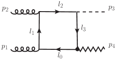
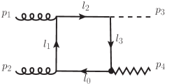
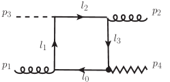
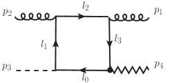
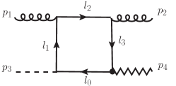
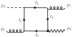
Figure 1: Box diagrams that contribute to the process $gg\to hG_{\rm KK}$. The graviton is denoted by the zigzag lines. All the external momenta are assumed to be incoming.

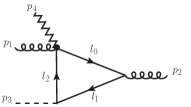
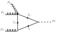
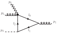
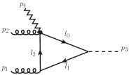
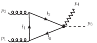
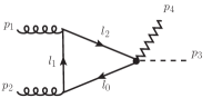
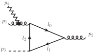
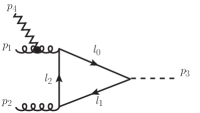
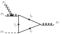
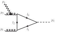
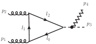
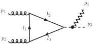
Figure 2: Triangle diagrams that contribute to the process $gg\to hG_{\rm KK}$. The zigzag lines denote the graviton. All the external momenta are assumed to be incoming. Class I diagrams, containing a quark-quark-boson-Graviton vertex (either $qqgG_{\rm KK}$ or $qqhG_{\rm KK}$), are shown in 2 - 2, and Class II diagrams, containing a boson-boson-Graviton vertex (either $ggG_{\rm KK}$ or $hhG_{\rm KK}$), are shown in 2 - 2.

Feynman rules for the vertices required to calculate these diagrams can be found in Ref. [10]. We display the amplitudes of two of the box diagrams and three triangle diagrams below. Amplitudes for other diagrams can be generated from these prototype diagrams by interchanging appropriate external momenta and polarization vectors.

2.1   Prototype Box Diagrams

The amplitude for the box diagram shown in Fig. 11 is given by,

$$\mathcal{M}^{ij}_{box(a)} = C^{ij}_{\rm G}\int\frac{d^{n}l_{0}}{(2\pi)^{n}}\;tr\left[(\not{l}_{0}+m_{t})V_{\rm qqG}^{\alpha\beta}(l_{3},l_{0})(\not{l}_{3}+m_{t})(\not{l}_{2}+m_{t})\gamma_{\mu_{2}}(\not{l}_{1}+m_{t})\gamma_{\mu_{1}}\right]$$ (10)

$$\times\frac{\varepsilon^{\mu_{1}}(p_{1})\varepsilon^{\mu_{2}}(p_{2})\varepsilon^{\rm G}_{\alpha\beta}(p_{4})}{D_{0}D_{1}D_{2}D_{3}},$$

where $i,j$ denote the color indices of the gluons, $\varepsilon$ is the polarization vector of a gluon, $\varepsilon^{\rm G}$ is the graviton polarization tensor, $D_{i}=l_{i}^{2}-m_{t}^{2}$, $n=4-2\epsilon$ and the coupling,

$$C^{ij}_{\rm G}=\frac{1}{8}g_{s}^{2}\kappa y_{t}\times\frac{\delta^{ij}}{2}.$$ (11)

All the vertex factors, $V$’s, are given in Appendix A. The amplitude of the diagram given in Fig. 11 can be obtained from this amplitude by permuting momenta and polarization vectors of the gluons. Similarly, the amplitude for the box diagram shown in Fig. 11 is given by,

$$\mathcal{M}^{ij}_{box(c)} = C^{ij}_{\rm G}\int\frac{d^{n}l_{0}}{(2\pi)^{n}}\;tr\left[(\not{l}_{0}+m_{t})V_{\rm qqG}^{\alpha\beta}(l_{3},l_{0})(\not{l}_{3}+m_{t})\gamma_{\mu_{2}}(\not{l}_{2}+m_{t})(\not{l}_{1}+m_{t})\gamma_{\mu_{1}}\right]$$ (12)

$$\times\frac{\varepsilon^{\mu_{1}}(p_{1})\varepsilon^{\mu_{2}}(p_{2})\varepsilon^{\rm G}_{\alpha\beta}(p_{4})}{D_{0}D_{1}D_{2}D_{3}}.$$

The other three box diagrams give contributions identical to the first three diagrams.

2.2   Prototype Triangle Diagrams

The amplitude for the triangle diagrams shown in Figs. 22, 22 and 22 in the Feynman gauge are given as,

$$\mathcal{M}^{ij}_{tri(a)} = -2C^{ij}_{\rm G}\int\frac{d^{n}l_{0}}{(2\pi)^{n}}\;tr\left[(\not{l}_{0}+m_{t})V_{\rm qqgG}^{\alpha\beta;\mu_{1}}(\not{l}_{2}+m_{t})(\not{l}_{1}+m_{t})\gamma^{\mu_{2}}\right]$$ (13)

$$\times\frac{\varepsilon_{\mu_{1}}(p_{1})\varepsilon_{\mu_{2}}(p_{2})\varepsilon^{\rm G}_{\alpha\beta}(p_{4})}{D_{0}D_{1}D_{2}},$$

$$\mathcal{M}^{ij}_{tri(g)} = -4C^{ij}_{\rm G}\int\frac{d^{n}l_{0}}{(2\pi)^{n}}\;tr\left[(\not{l}_{0}+m_{t})\gamma_{\rho}(\not{l}_{2}+m_{t})(\not{l}_{1}+m_{t})\gamma^{\mu_{2}}\right]$$ (14)

$$\times\frac{V_{\rm ggG}^{\alpha\beta;\mu_{1}\rho}(p_{1},p_{2}+p_{3})}{(p_{2}+p_{3})^{2}}\times\frac{\varepsilon_{\mu_{1}}(p_{1})\varepsilon_{\mu_{2}}(p_{2})\varepsilon^{\rm G}_{\alpha\beta}(p_{4})}{D_{0}D_{1}D_{2}},$$

$$\mathcal{M}^{ij}_{tri(k)} = -4C^{ij}_{\rm G}\int\frac{d^{n}l_{0}}{(2\pi)^{n}}\;tr\left[(\not{l}_{0}+m_{t})(\not{l}_{2}+m_{t})\gamma^{\mu_{2}}(\not{l}_{1}+m_{t})\gamma^{\mu_{1}}\right]$$ (15)

$$\times\frac{V_{\rm hhG}^{\alpha\beta}(p_{1}+p_{2},p_{3})}{(p_{1}+p_{2})^{2}-m_{h}^{2}}\times\frac{\varepsilon_{\mu_{1}}(p_{1})\varepsilon_{\mu_{2}}(p_{2})\varepsilon^{\rm G}_{\alpha\beta}(p_{4})}{D_{0}D_{1}D_{2}}.$$

The contribution of all other triangle diagrams can be obtained by appropriate permutations of the momenta and polarization vectors.

To compute these amplitudes, we first compute the traces associated with the top quark loop by using symbolic manipulation program, FORM [27]. At this stage, the amplitude contains tensor integrals, 4-rank tensor-box integral ($D^{\mu\nu\rho\sigma}$) being the most complicated one,

$$D^{\mu\nu\rho\sigma}=\int\frac{d^{n}l_{0}}{(2\pi)^{n}}\frac{l_{0}^{\mu}l_{0}^{\nu}l_{0}^{\rho}l_{0}^{\sigma}}{D_{0}D_{1}D_{2}D_{3}}.$$ (16)

We reduce the tensor integrals into the standard scalar integrals – $A_{0}$, $B_{0}$, $C_{0}$ and $D_{0}$ [28] using the reduction scheme developed by Oldenborgh and Vermaseren [29]. The algorithm described in Ref. [29] was first coded using Mathematica. Then after the reduction, appropriate Fortran routines were obtained [30]. After the full reduction the amplitude has the following generic structure,

$$\mathcal{M}=\sum_{i}\left(d_{i}D_{0}^{i}\right)+\sum_{i}\left(c_{i}C_{0}^{i}\right)+\sum_{i}\left(b_{i}B_{0}^{i}\right)+\sum_{i}\left(a_{i}A_{0}^{i}\right)+\mathcal{R},$$ (17)

where $\mathcal{R}$ is the rational term coming from the UV regularization of tensor integrals and the index $i$ stands for different momentum combinations that enter in these scalars. All the needed scalar integrals (with massive internal lines) are called from FF library [31]. The amplitude is thus a function of external momenta and polarizations. We consider the helicity basis for the polarization vectors to calculate the amplitude. We explicitly check the symmetries of the helicity amplitudes to ensure the correctness of our calculation.

With the above amplitude, we perform integrations over the two body phase space, momentum fractions ($x_{1}/x_{2}$) of the initial state gluons and over the graviton mass parameter in the continuum approximation (for the ADD model). As a cautionary check, we have performed a few tests with our program. The amplitude should be free of divergences and also be gauge invariant. Because of the massive top quark in the loop, there are no infrared divergences. We have checked the UV finiteness and gauge invariance.

1. UV Finiteness: Individual box and triangle diagrams can be UV divergent, but the total amplitude should be UV finite. We have tested the UV finiteness of the total amplitude by varying the renormalization scale ($\mu_{\rm R}$) over ten orders of magnitude. We find that the amplitude is independent of the actual value of $\mu_{\rm R}$. The triangle and box amplitudes are separately UV finite. In fact, each triangle diagram is UV finite by itself. This behavior is similar to that of the $gg\to h$ amplitude which is UV finite.

2. Gauge Invariance: We have checked the gauge invariance of the amplitude with respect to both the gluons. This has been done by replacing the polarization vector of either of the gluons by its momentum ($\varepsilon^{\mu}(p_{i})\to p^{\mu}_{i}$). This, as expected, makes the amplitude zero. We observe that some of the triangle diagrams are separately gauge invariant with respect to both the gluons. To ensure the correctness of their contribution toward the full amplitude, we perform gauge invariance check with respect to the graviton polarization also.

2.3   Calculation in the Effective Theory

It is well known that in the SM it is possible to integrate out the top quark loop contribution to the $gg\to h$ process in the heavy quark limit, i.e., $m_{t}\gg m_{h}/2$ and describe the Higgs-gluon interaction by an effective Lagrangian [32],

$$\mathcal{L}_{\rm eff}=-\frac{1}{4}g_{h}\,G^{a}_{\mu\nu}G^{a\,\mu\nu}h\,,$$ (18)

where $G^{a}_{\mu\nu}$ is the gluon field-strength tensor. The effective coupling, $g_{h}$ is given as,

$$g_{h}=\frac{\alpha_{s}}{3\pi v}\left[1+\mathcal{O}(\tau_{h})\right]\,,$$ (19)

where $\tau_{h}=m^{2}_{h}/4m_{t}^{2}$ and $v$ is the vacuum expectation value of the Higgs boson field. In principle, one can compute the $gg\to hG_{\rm KK}$ process also using this effective theory. Within this theory the diagrams that contribute are shown in Fig. 3. The vertex factor for the diagram in Fig. 3 can be obtained by computing the contribution of the Lagrangian given in Eq. 18 to the stress-energy tensor. It is given in Appendix C.

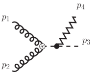
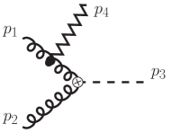
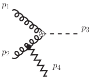
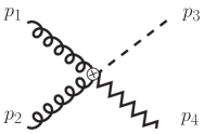
Figure 3: Diagrams that contribute to the process $gg\to hG_{\rm KK}$ in the effective theory.

3   Results

In this section we present the numerical results for the LHC with $\sqrt{s}=14$ TeV. The ADD model has two parameters – the cut-off scale, $M_{\rm S}$, and the number of extra dimensions, $d$. We find the dependence of the cross section on these parameters. In addition to these parameters, the cross section also depends on the choice of the parton distribution functions and the choice of renormalization/factorization scale. We choose the LO CTEQ6L1 PDFs[33]. For the factorization/renormalization scale, we choose the transverse mass of the Higgs boson, $\sqrt{m_{h}^{2}+\left(p^{h}_{\rm T}\right)^{2}}$. Later we comment on the dependence of the cross section on the choice of PDF’s or the factorization/renormalization scale.

To compute the cross section, we apply the following cuts on the transverse momentum and rapidity of the Higgs boson: $p_{\rm T}^{h}>20$ GeV, $|\eta^{h}|<2.5$. In case of the ADD model, we apply one extra cut on the invariant mass of the outgoing particles: $M(hG_{\rm KK})\leq M_{\rm S}$. This is the truncated scheme[11]. Later, we also comment on the untruncated scheme.

Figure 4: Variation of the cross section ($\sigma$) with the mass of the Higgs boson ($m_{h}$) in the ADD model. Here the cutoff scale, $M_{\rm S}=2$ TeV and number of extra dimensions, $d=2$. In the lower part of the plot we show the $b$-loop contribution ($\sigma_{b}$) to $\sigma$ as percentage of it. The line is a linear fit for the points.

Figure 5: Variation of the cross section ($\sigma$) with the cutoff scale ($M_{\rm S}$) of the ADD model for different numbers of extra dimensions, $d$. For this plot the Higgs mass, $m_{h}=120$ GeV.

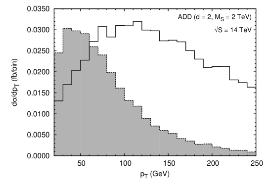
Figure 6: Distribution of the transverse momentum of the Higgs boson in the ADD model for $d=2$ and $M_{\rm S}$ = 2 TeV. Here the Higgs mass, $m_{h}=120$ GeV. The shaded curve is the $p_{\rm T}$ distribution of the Higgs for the SM background $pp\to hZ$ with Z decaying into pair of neutrinos obtained using Madgraph5 [35]. The background curve is scaled by a factor of 500.

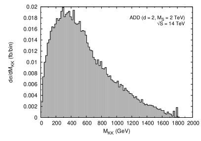
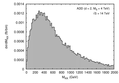
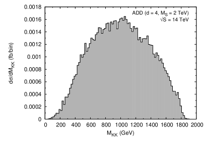
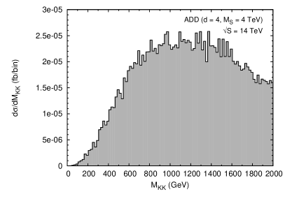
Figure 7: Relative contributions of different KK modes in the ADD model for different cutoff scales and numbers of extra dimensions – (a) $d=2$, $M_{\rm S}$ = 2 TeV, (b) $d=2$, $M_{\rm S}$ = 4 TeV, (c) $d=4$, $M_{\rm S}$ = 2 TeV and (d) $d=4$, $M_{\rm S}$ = 4 TeV. For these plots the Higgs mass, $m_{h}=120$ GeV.

Figure 8: Dependence of the cross section ($\sigma$) for the ADD model on the center of mass energy of the collider. For this plot $M_{\rm S}$ = 2 TeV, $d=2$ and $m_{h}$ = 120 GeV.

In Fig. 4, we show how the cross section changes with the Higgs boson mass, $m_{h}$. Here the cutoff scale, $M_{\rm S}$ has been set to 2 TeV and the number of compactified extra dimensions is 2. The cross section decreases with increasing Higgs boson mass primarily due to phase-space suppression. We see that over most of the plotted range, the cross section varies from about $0.9$ to $0.5$ fb. From this figure we also see that the bottom quark loop contribution to the cross-section is negligible – less than a percent (for the case of $gg\to h$ in the SM see [34]). In Fig. 5, we show the dependence of the cross section on the scale, $M_{\rm S}$ for different values of $d$. In Fig. 6, we have plotted the transverse momentum distribution of the Higgs boson for $d=2$ and $M_{\rm S}$ = 2 TeV. We see that it has a peak at about 120 GeV. In Fig. 7, we have plotted the dependence of the cross section on the $G_{\rm KK}$ mass for different values of $M_{\rm S}$ and $d$. Since the density of graviton states increases with the increase in the mass of the graviton, the cross section gets contribution from mostly large values of the $G_{\rm KK}$ mass. For example for $d=2$ the peaks of the curves lie around 400 GeV (see Figs. 7 and 7). However at the end phase space suppression takes over and the cross section starts to decrease. From Eq. 4 one would also expect this value to increase with the increase in $d$. This is seen in Figs. 7 and 7, where for $d=4$ the peaks lie around 1 TeV. In Fig. 8 we show how the cross section increases with increasing center of mass energy of the collider.

We see that for the parameter ranges considered the cross section is much smaller than what one would roughly estimate. To see that let us consider the SM process $gg\to h$ via a top quark loop (LO). For 14 TeV LHC and $m_{h}\sim 120$ GeV the cross section of this process is about $20-25$ pb [36]. If one ignores the phase space suppression due to the extra graviton, one would roughly expect the $gg\to hG_{\rm KK}$ process to be suppressed compared to the $gg\to h$ process by an extra factor of $(E/M_{\rm S})^{(d+2)}$ where $E$ is the energy scale of the process. From Fig. 7 we see that the maximum contribution comes from KK modes with mass $\sim$ 400 GeV. Hence if one takes $E\approx\sqrt{\hat{s}}\approx 500$ GeV, then for $M_{\rm S}=2$ TeV and $d=2$, one would expect the cross section to be about 80 fb compared to 0.8 fb that we get (see Fig. 4). This happens because of the destructive interference between the contributions coming from the box-diagrams and the triangle-diagrams which happens because of the relative negative sign between these two sets of diagrams. This cancellation reduces the amplitude drastically. For example, for $d=2$, $M_{\rm S}=2$ TeV and $m_{h}=120$ GeV, switching off the box diagrams leads to a cross section of 158805.5 fb – i.e.. a increase of six orders of magnitude in the cross section. This roughly translates in to a cancellation of about two or three orders of magnitude at the amplitude level. This cancellation and the cuts applied on physical quantities reduces the cross section to such small values. Still, one would expect a few hundred such events after the LHC achieves its design luminosity.

Figure 9: Variation of the cross section ($\sigma$) with $m_{t}$ in the ADD model. For this plot the cutoff scale, $M_{\rm S}=2$ TeV and the number of extra dimensions, $d=2$. The effective theory contribution is also shown.

Another interesting feature that we can see is that there is no decoupling of the top quark in the loop[37]. For this purpose, we have varied $m_{t}$ from 50 GeV to 5 TeV. From Fig. 9 we clearly see that in the beginning the cross section increases due to the propagator enhancement. However, beyond $m_{t}\approx 400$ GeV, cross section decreases and approaches a constant value beyond $m_{t}\gtrsim 2$ TeV. This behavior is similar to what has been seen in the case of $gg\to h$ production within the SM. In the large $m_{t}$ limit, there also cross section is independent of $m_{t}$[38]. In the SM, because of the Higgs mechanism, we don’t necessarily expect complete decoupling of the heavy quarks, as it exists in the case of QED and QCD. In Fig. 9 we also show the cross section computed using the effective theory approximation as described in Sec. 2.3. In the numerical computation we keep upto $\mathcal{O}(\tau_{h}^{3})$ terms which account for the $m_{t}$ dependence of the cross section for small $m_{t}$. The two calculations agree very well for $m_{t}\geq 1.2$ TeV. However for $m_{h}=120$ GeV and the physical top quark mass these two differ. This can also be seen from Fig. 10. This is unlike the SM $gg\to h$ case where this approximation works quite well [39]. However in our case, there is one extra scale present – namely, the mass of the graviton, $M_{\rm KK}$. We have seen that the $M_{\rm KK}$ value is significantly larger than the mass of the top quark most of the time. Because of this, $\sqrt{\hat{s}}$, which is larger than $m_{h}+M_{\rm KK}$, can go much beyond $2m_{t}$. Therefore, one cannot expect the effective theory calculation to agree with the full calculation for $m_{h}=120$ GeV and the physical top quark mass.

Figure 10: Comparison between the effective theory and the full calculation. Here $m_{t}=175$ GeV.

By using different CTEQ parton distributions CTEQ6M, CTEQ6D or CTEQ6L, we find that the cross section can change by $5-15$ percent. We have also varied the factorization/renormalization scale by a factor of two. We find that the cross section can vary by $20-25$ percent. This variation can only be reduced by computing radiative correction to this process. For $d=2$ and $M_{\rm S}=2$ TeV, the difference in the truncated and untruncated scheme cross sections is about $15\%$ for $m_{h}=120$ GeV. This difference increases to about $60\%$ for $d=4$. Furthermore, this difference keeps decreasing with the increase in the cut-off scale $M_{\rm S}$. These results are consistent with the observation made in Refs.[24, 25]. Our results will be modified if we include the QCD corrections to this process. Our process shares many features with the process $gg\to h$. Therefore one may expect significant QCD corrections, i.e, a K-factor of the order of 2.

Figure 11: Variation of the cross section ($\sigma$) scaled with the square of the dimensionless coupling $c_{0}=k/{\bar{M}_{\rm PL}}$ with the mass of the Higgs ($m_{h}$) for different values of $M_{1}$ – mass of the first KK mode of the graviton – in the RS model.

We have also computed the cross section for the RS model. In Fig. 11, we have plotted the scaled cross section for three different values of the mass of the first KK mode of the graviton. We see that, for $0.01\lesssim c_{0}\lesssim 0.1$, the cross section is more than an order of magnitude smaller than that in the ADD model. For example for $c_{0}=0.075$, $M_{1}=1$ TeV and $m_{h}=120$ GeV the cross section is only about 0.02 fb. The cross section is only significant for the smaller value of $M_{1}$ (correspondingly $m_{0}$) and larger value of $c_{0}$.

The question arises now – can this process be observed at the LHC (assuming that both particles exist)? To answer this one needs to understand the background. However, a complete analysis of the backgrounds is beyond the scope of this paper. We would discuss the possible signatures of this process semi-quantitatively. For $M_{\rm S}=2$ TeV and $d=2$, the cross section is of the order of a fb for the mass range $m_{h}=110-200$ GeV. In this mass range, the major decay modes of the Higgs boson are $h\to b{\bar{b}},WW,ZZ$. We will also take that graviton is not observed and it gives rise to a large missing $p_{\rm T}$ which can be used as a possible discriminator between the signal and the background. This can be seen from the the $p_{\rm T}$ distributions, shown in Fig. 6. For our process, the $p_{\rm T}$ of the graviton is same as that for the Higgs by the momentum conservation.

Let us now consider the signal and the backgrounds from the SM process for various major decay modes of the Higgs boson.

1. $h\to b{\bar{b}}$: This decay mode is dominant up-to about $m_{h}\approx 135$ GeV. In the case of this decay mode, the signal will be “two-$b$ jets + large missing $p_{\rm T}$”. The main source of the background would be the production of ZZ pair and $Z+b{\bar{b}}$. The typical cross section for $pp\to ZZX$ is about 10 pb. This is about four-orders of magnitude higher than the signal cross section. The cross section for $Z+b{\bar{b}}$ production, with $Z$-boson decaying into neutrinos, is also of the order of $10$ pb. One can suppress the backgrounds by considering the large missing $p_{\rm T}$ and demanding the mass $M(b\bar{b})$ to be around the mass of the Higgs boson. With the branching ratios of the $Z$ decays, we may be able to gain about two-three orders of magnitude in the signal-to-background ratio. Because of the small cross sections, it may require many years of LHC run before this process could be seen through this decay mode of the Higgs boson.

2. $h\to W^{+}W^{-}$: This decay mode is important for $m_{h}\gtrsim 135$ GeV. The signature of this process can be “two-leptons and large missing $p_{\rm T}$” or “one-lepton + 2 jets + large missing $p_{\rm T}$”. The main sources of the backgrounds would be the production of WWZ and ZZ bosons. The typical cross section for the background $pp\to WWZX$ is about $100$ fb. The ZZ background can be suppressed as the lepton pair from the Z-decay will have mass around $M_{\rm Z}$, while the lepton-pair from the signal will have continuum distribution. The other background WWZ production can also be reduced using larger missing $p_{\rm T}$ cut and the difference in $M(\ell\ell)$ distributions. Observation of this decay mode may also take several years.

3. $h\to ZZ$: For $m_{h}\gtrsim 175$ GeV, this is the most important decay mode. For the SM Higgs boson production $gg\to h$, this decay mode gives rise to gold-plated signature of the “two-lepton pairs”. In our case, this decay mode will give rise to two Z-bosons and large missing $p_{\rm T}$ in the final state. The signal could be “four-lepton + large missing $p_{\rm T}$”, or “ two leptons + two jets + large missing $p_{\rm T}$”. The main background is $pp\to ZZZX$ process. The typical cross section for this process is about 11 fb. To get large missing $p_{\rm T}$, one of the Z-boson will have to decay into neutrinos which has a branching ratio of about $20\%$. Using the large missing $p_{\rm T}$ and the mass of the two-lepton pairs (i.e. four leptons), this decay channel will give rise to the best observable signature of the process $gg\to hG_{\rm KK}$.

4   Conclusions

In this paper, we have computed cross section and distributions for the process $pp\to hG_{\rm KK}\,X$ for $m_{h}=110-200$ GeV. This process occurs at the one-loop level through gluon-gluon fusion $gg\to hG_{\rm KK}$. The loop diagrams have been computed using the Oldenborgh-Vermaseren tensor-integral reduction procedure. We have presented the calculation in the ADD model, with a brief discussion in the context of the RS model. In the case of the ADD model, the cross section can be of the order of one fb. These values are smaller than expected due to destructive interference between the box-class and triangle-class of diagrams. This destructive interference reduces the amplitude by about two-orders of magnitude. The contribution to the cross section is mostly from large values of $M_{\rm KK}$.We also note that the top quark does not decouple in the heavy top quark mass limit. We have also performed the computation using the effective theory approach. Only for very large top quark mass this result matches very well with the exact calculation. We find that the cross sections in the RS model are quite small. For $c_{0}=0.075$ and $M_{1}=1$ TeV, the cross section is about $0.02$ fb. We have also briefly considered possible signatures of this process. It appears that for larger $m_{h}$, in the case of the ADD model, one may be able to observe this process at the LHC after a run of a few years.

Acknowledgments
AS wants to thank M. Serone and I. Rothstein for fruitful discussions.

Appendix A   Graviton Vertex Factors

The graviton vertex factors used in the calculation are

$$V_{\rm qqG}^{\alpha\beta}(k_{1},k_{2}) = \gamma^{\alpha}(k_{1}^{\beta}+k_{2}^{\beta})+\gamma^{\beta}(k_{1}^{\alpha}+k_{2}^{\alpha}),$$ (A.1)

$$V_{\rm hhG}^{\alpha\beta}(k_{1},k_{2}) = C^{\alpha\beta;\rho\sigma}\,k_{1\rho}k_{2\sigma},$$ (A.2)

$$V_{\rm ggG}^{\alpha\beta;\rho\sigma}(k_{1},k_{2}) = (k_{1}\cdot k_{2})C^{\alpha\beta;\rho\sigma}+D^{\alpha\beta;\rho\sigma}(k_{1},k_{2})+\frac{1}{\xi}E^{\alpha\beta;\rho\sigma}(k_{1},k_{2}),$$ (A.3)

$$V_{\rm qqgG}^{\alpha\beta;\rho} = C^{\alpha\beta;\rho\sigma}\,\gamma_{\sigma}.$$ (A.4)

For our computation, we have used the Feynman gauge, i.e., $\xi=1$. The definitions of the functions $C$, $D$ and $E$ can be found in Ref. [10], which are

$$C^{\alpha\beta;\rho\sigma} = \eta^{\alpha\rho}\eta^{\beta\sigma}+\eta^{\alpha\sigma}\eta^{\beta\rho}-\eta^{\alpha\beta}\eta^{\rho\sigma},$$ (A.5)

$$D^{\alpha\beta;\rho\sigma}(k_{1},k_{2}) = \eta^{\alpha\beta}k_{1}^{\sigma}k_{2}^{\rho}-\biggl{[}\eta^{\alpha\sigma}k_{1}^{\beta}k_{2}^{\rho}+\eta^{\alpha\rho}k_{1}^{\sigma}k_{2}^{\beta}-\eta^{\rho\sigma}k_{1}^{\alpha}k_{2}^{\beta}+(\alpha\leftrightarrow\beta)\biggr{]},\quad$$ (A.6)

$$E^{\alpha\beta;\rho\sigma}(k_{1},k_{2}) = \eta^{\alpha\beta}(k_{1}^{\rho}k_{1}^{\sigma}+k_{2}^{\rho}k_{2}^{\sigma}+k_{1}^{\rho}k_{2}^{\sigma})$$ (A.7)

$$\quad\quad\quad\quad-\biggl{[}\eta^{\beta\sigma}k_{1}^{\alpha}k_{1}^{\rho}+\eta^{\beta\rho}k_{2}^{\alpha}k_{2}^{\sigma}+(\alpha\leftrightarrow\beta)\biggr{]}.$$

Appendix B   The $hqqG_{\rm KK}$ Vertex

The $hqqG^{\vec{n}}_{\rm KK}$ vertex, proportional to the Yukawa coupling ($y_{q}$) for a quark $q$, can be written as:

$$\tilde{h}_{\alpha\beta}^{\vec{n}}\bar{\psi}\psi\Phi : \frac{i}{2}\,y_{q}\,\kappa\,\eta_{\alpha\beta}\,\delta_{mn}$$ (B.1)

$$\tilde{\phi}_{ij}^{\vec{n}}\bar{\psi}\psi\Phi : -2i\,\omega\,y_{q}\,\kappa\,\delta_{ij}\,\delta_{mn}$$ (B.2)

where we have followed the notation of Ref. [10]. The Yukawa coupling is given as,

$$y_{q} = -\frac{g}{2m_{W}}\,m_{q}.$$ (B.3)

Appendix C   The $hggG_{\rm KK}$ Vertex in the Effective theory

The $hggG_{\rm KK}$ vertex is given by:

$$\tilde{h}_{\mu\nu}^{\vec{n}}gg\Phi : \frac{i\kappa}{2}\,g_{h}\,\delta_{ab}\,\left[\left(p_{1}\cdot p_{2}\right)C^{\mu\nu;\rho\sigma}+D^{\mu\nu;\rho\sigma}(p_{1},p_{2})\right]\,.$$ (C.1)

References

- [1] K. Nakamura et al. [Particle Data Group], J. Phys. G 37, 075021 (2010).
- [2] J. D. Lykken, arXiv:1005.1676 [hep-ph] and the references therein.
- [3] J. Ellis, arXiv:1102.5009 [hep-ph].
- [4] N. Arkani-Hamed, S. Dimopoulos and G. R. Dvali, Phys. Lett. B 429, 263 (1998); [arXiv:hep-ph/9803315].
- [5] L. Randall and R. Sundrum, Phys. Rev. Lett. 83, 3370 (1999); [arXiv:hep-ph/9905221].
- [6] L. Randall and R. Sundrum, Phys. Rev. Lett. 83, 4690 (1999); [arXiv:hep-th/9906064].
- [7] I. Antoniadis, Phys. Lett. B 246, 377 (1990).
- [8] T. Appelquist, H. C. Cheng and B. A. Dobrescu, Phys. Rev. D 64, 035002 (2001); [arXiv:hep-ph/0012100].
- [9] H. Davoudiasl, J. L. Hewett, T. G. Rizzo, Phys. Rev. Lett. 84, 2080 (2000); [arXiv:hep-ph/9909255].
- [10] T. Han, J. D. Lykken and R. J. Zhang, Phys. Rev. D 59, 105006 (1999); [arXiv:hep-ph/9811350].
- [11] G. F. Giudice, R. Rattazzi, J. D. Wells, Nucl. Phys. B544, 3-38 (1999). [hep-ph/9811291].
- [12] E. A. Mirabelli, M. Perelstein and M. E. Peskin, Phys. Rev. Lett. 82, 2236 (1999) [arXiv:hep-ph/9811337].
- [13] D. K. Ghosh, S. Raychaudhuri, Phys. Lett. B495, 114-120 (2000); [arXiv:hep-ph/0007354].
- [14] T. Kaluza, Sitzungsber. Preuss. Akad. Wiss. Berlin (Math. Phys. ) 1921, 966 (1921).
- [15] O. Klein, Z. Phys. 37, 895 (1926) [Surveys High Energ. Phys. 5, 241 (1986)].
- [16] D. J. Kapner, T. S. Cook, E. G. Adelberger, J. H. Gundlach, B. R. Heckel, C. D. Hoyle and H. E. Swanson, Phys. Rev. Lett. 98, 021101 (2007); [arXiv:hep-ph/0611184].
- [17] S. Chatrchyan et al. [CMS Collaboration], JHEP 1105, 085 (2011); [arXiv:1103.4279 [hep-ex]].
- [18] W. D. Goldberger, M. B. Wise, Phys. Rev. D60, 107505 (1999); [arXiv:hep-ph/9907218].
- [19] P. Mathews, V. Ravindran, K. Sridhar, JHEP 0510, 031 (2005); [arXiv:hep-ph/0506158].
- [20] T. Aaltonen et al. [CDF Collaboration], Phys. Rev. Lett. 107, 051801 (2011); [arXiv:1103.4650 [hep-ex]].
- [21] V. M. Abazov et al. [The D0 Collaboration], Phys. Rev. Lett. 104, 241802 (2010); [arXiv:1004.1826 [hep-ex]].
- [22] M. C. Kumar, P. Mathews, V. Ravindran, S. Seth, J. Phys. G G38, 055001 (2011); [arXiv:1004.5519 [hep-ph]].
- [23] M. C. Kumar, P. Mathews, V. Ravindran, S. Seth, Nucl. Phys. B847, 54-92 (2011); [arXiv:1011.6199 [hep-ph]].
- [24] S. Karg, M. Kramer, Q. Li, D. Zeppenfeld, Phys. Rev. D81, 094036 (2010); [arXiv:0911.5095 [hep-ph]].
- [25] X. Gao, C. S. Li, J. Gao, J. Wang and R. J. Oakes, Phys. Rev. D 81, 036008 (2010) [arXiv:0912.0199 [hep-ph]].
- [26] A. Shivaji, V. Ravindran and P. Agrawal, arXiv:1111.6479 [hep-ph].
- [27] J. A. M. Vermaseren, arXiv:math-ph/0010025.
- [28] G. ’t Hooft and M. J. G. Veltman, Nucl. Phys. B 153, 365 (1979).
- [29] G. J. van Oldenborgh and J. A. M. Vermaseren, Z. Phys. C 46, 425 (1990).
- [30] P. Agrawal and G. Ladinsky, Phys. Rev. D 63, 117504 (2001); [arXiv:hep-ph/0011346].
- [31] G. J. van Oldenborgh, Comput. Phys. Commun. 66, 1 (1991).
- [32] T. G. Rizzo, Phys. Rev. D 22, 178 (1980) [Addendum-ibid. D 22, 1824 (1980)].
- [33] J. Pumplin, D. R. Stump, J. Huston, H. L. Lai, P. M. Nadolsky and W. K. Tung, JHEP 0207, 012 (2002); [arXiv:hep-ph/0201195].
- [34] C. Anastasiou, S. Bucherer and Z. Kunszt, JHEP 0910, 068 (2009) [arXiv:0907.2362 [hep-ph]].
- [35] J. Alwall, M. Herquet, F. Maltoni, O. Mattelaer and T. Stelzer, JHEP 1106, 128 (2011) [arXiv:1106.0522 [hep-ph]].
- [36] A. Djouadi, Phys. Rept. 457, 1 (2008) [arXiv:hep-ph/0503172].
- [37] T. Appelquist and J. Carazzone, Phys. Rev. D 11, 2856 (1975).
- [38] H. M. Georgi, S. L. Glashow, M. E. Machacek and D. V. Nanopoulos, Phys. Rev. Lett. 40, 692 (1978).
- [39] A. Pak, M. Rogal and M. Steinhauser, JHEP 1002, 025 (2010) [arXiv:0911.4662 [hep-ph]].