Partially Screened Gap - general approach and observational consequences

Abstract:

Observations of the thermal X-ray emission from radio pulsars implicate that the size of hot spots is much smaller then the size of the polar cap that follows from the purely dipolar geometry of pulsar magnetic field. Most plausible explanation of this phenomena is an assumption that the magnetic field at the stellar surface differs essentially from the purely dipolar field. We can determine magnetic field at the surface by the conservation of the magnetic flux through the area bounded by open magnetic field lines. Then the value of the surface magnetic field can be estimated as of the order of $10^{14}$ G. On the other hand observations show that the temperature of the hot spot is about a few million Kelvins. Based on these observations the Partially Screened Gap (PSG) model was proposed which assumes that the temperature of the actual polar cap (hot spot) equals to the so called critical temperature.

We discuss correlation between the temperature and corresponding area of the thermal X-ray emission for a number of pulsars. The results of our analysis show that the PSG model is suitable to explain both cases: when the hot spot is smaller and larger then conventional polar cap. We argue that in the second case structure and curvature of field lines allow pair creation in the closed field lines region thus the secondary particles can heat the stellar surface outside the actual polar cap.

We have found that the Curvature Radiation (CR) plays dominant role in avalanche pair production in the PSG. We studied dependence of the PSG parameters on the pulsar period, the magnetic field strength and the curvature of field lines.

1 Introduction

The Standard model of radio pulsars assumes that there exists the Inner Acceleration Region (IAR) above the polar cap where the electric field has a component along the opened magnetic field lines. In this region particles (electrons and positrons) are accelerated in both directions: outward and toward the stellar surface. Consequently, outflowing particles are responsible for generation of the magnetospheric emission (radio and high-frequency) while the backflowing particles heat the surface and provide required energy for the thermal emission. In such scenario analysis of X-ray radiation is an excellent method to get insight into the most intriguing region of the neutron star.

1.1 Observations

About 30 years ago the first X-ray telescope called Einstein was put into space thus opening the possibility for direct investigation of thermal emission from isolated neutron stars. A significant contribution to this study was provided by ROSAT in 1990’s. Currently operating observatories such as Chandra and XMM-Newton have greatly increased the quality and availability of observations of thermal radiation from neutron star surfaces.

The X-ray radiation from an isolated neutron star in general can consist of two distinguishable components: the nonthermal emission and the thermal emission. The nonthermal component is usually described by a power-law spectral model and attributed to radiation produced in the pulsar magnetosphere while the thermal emission can originate either from the entire surface of cooling neutron star or the small hot spots around the magnetic poles on stellar surface (polar caps and adjacent areas).

Thermal X-ray emission seems to be a quite common feature of radio pulsars. The black body fit allows us to obtain directly the temperature ($T_{s}$) of the hot spot. Using the distance ($D$) to the pulsar and the luminosity of thermal emission ($L_{\rm bol}$) we can estimate the area ($A_{\rm BB}$) of the hot spot. In the most cases $A_{\rm BB}$ differs from the conventional polar cap area $A_{\rm pc}\approx 6.2\times 10^{4}P^{-1}$ m², where $P$ is pulsar period. We use parameter $b=A_{\rm pc}/A_{\rm BB}$ to describe the difference between $A_{\rm pc}$ and $A_{\rm BB}$.

1.2 The case with $b<1$

In the most cases observed hot spot area ($A_{\rm BB}$) is larger then the conventional polar cap area. We can distinguish two types of pulsars in this group, with $b\ll 1$ and $b\lesssim 1$.

The first type is associated with observations of thermal emission from the entire stellar surface and can be used to test cooling models. Although we have to remember that for young pulsars ($\tau=1$ kyr) the nonthermal component dominates, making it impossible to measure accurately the thermal flux. As a pulsar becomes older, its nonthermal luminosity decreases faster then the thermal luminosity up to the end of the neutrino-cooling era ($\tau\sim 1$ Myr). Thus, the thermal radiation from the entire stellar surface can dominate at soft X-ray energies for middle-age pulsars ($\tau\sim 100$ kyr) and some younger pulsars ($\tau\sim 10$ kyr) [2].

Some observations show that the hot spot area is larger then the conventional polar cap area but still significantly less then the area of the star. In this case the radiation comes from the surface adjacent to polar cap. Therefore, it can not be explained by cooling of the surface and some addition heating mechanism is needed. The model of such heating is based on the assumption that the pulsar magnetic field near the stellar surface differs significantly from the pure dipole one. The calculations show that it is natural to obtain such geometry of magnetic field lines that allows the pair creation in the closed field lines region. The pairs move along closed magnetic field lines and heat the surface beyond the polar cap on the opposite side of the star (Fig. 1). In such scenario heating energy is generated in IAR (outward particles) hence the luminosity should be same order as the nonthermal one but it is hard to predict which of them would prevail in X-ray flux of an old neutron star. However, it cannot be ruled out that the thermal one may be dominant as suggested by some observations. In most cases area of a such heated surface may be larger (but not necessarily) then the conventional polar cap area. That makes the estimation of parameters of black-body radiation even harder. More detailed description of this phenomenon can be found in [3].

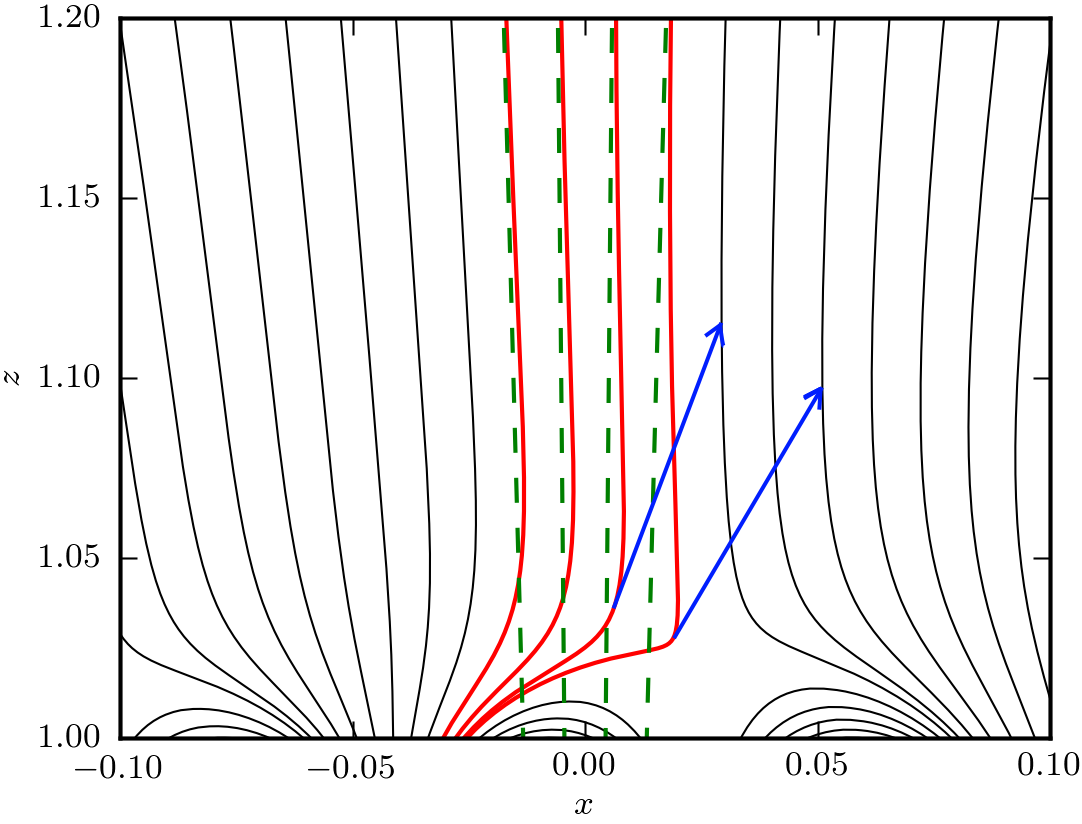
Figure 1: Cartoon of the magnetic field lines in the polar cap region. Red lines are open field lines and green dashed lines correspond to the dipole field. The blue arrows show direction of the curvature photons emission.

1.3 The case with $b>1$

In some cases observed hot spot area ($A_{\rm BB}$) is less then the conventional polar cap area ($b>1$). The model mentioned in 1.2 can be used in order to explain this phenomenon, because the size of modified polar cap is much smaller then size of conventional polar cap (see Fig. 1). The surface magnetic filed can be estimated by the magnetic flux conservation law as $b=A_{\rm pc}/A_{\rm BB}$ = $B_{s}/B_{d}$. Where $B_{d}=2.02\times 10^{12}(P\dot{P}_{-15})^{0.5}$, $P$ is the pulsar period in seconds and $\dot{P}_{-15}=\dot{P}/10^{-15}$ is the period derivative.

Medin & Lai [4] calculated the condition for the formation of a vacuum gap above neutron star surface. In Fig. 2 we present positions of pulsars with derived surface temperature ($T_{s}$) and hot spot area ($A_{\rm BB}$) on the $B_{s}-T_{s}$ diagram where $B_{s}$ is estimated as $B_{s}=bB_{d}$. Red line represents dependence of $T_{\rm crit}$ on $B_{s}$. We can see that in most cases the pulsars positions follow with $B_{s}-T_{\rm crit}$ theoretical curve. Few cases which do not coincide with the theoretical curve can be explained by heating the surface outside the polar cap (see 1.2).

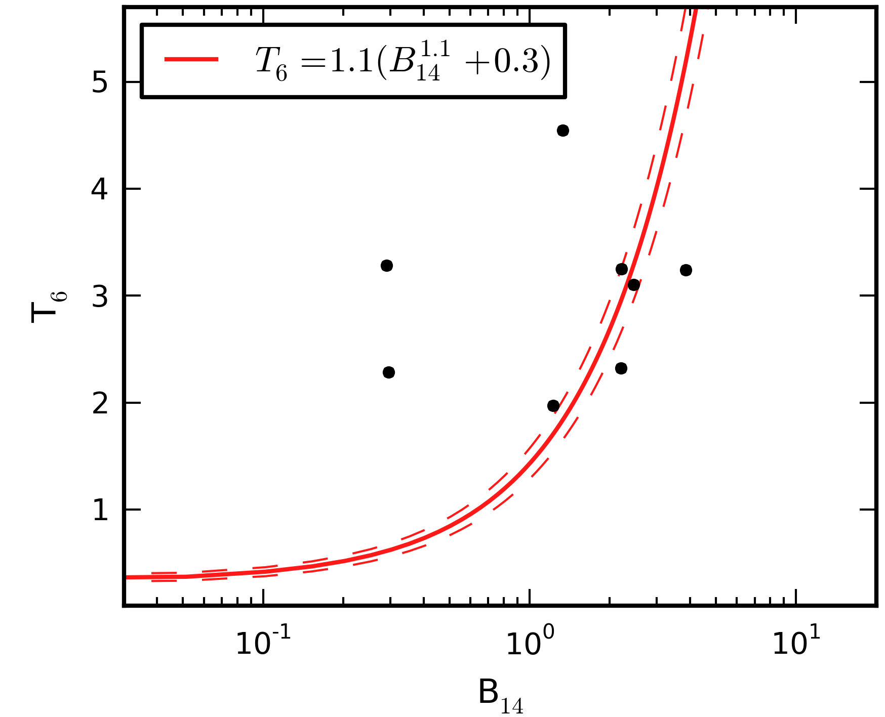
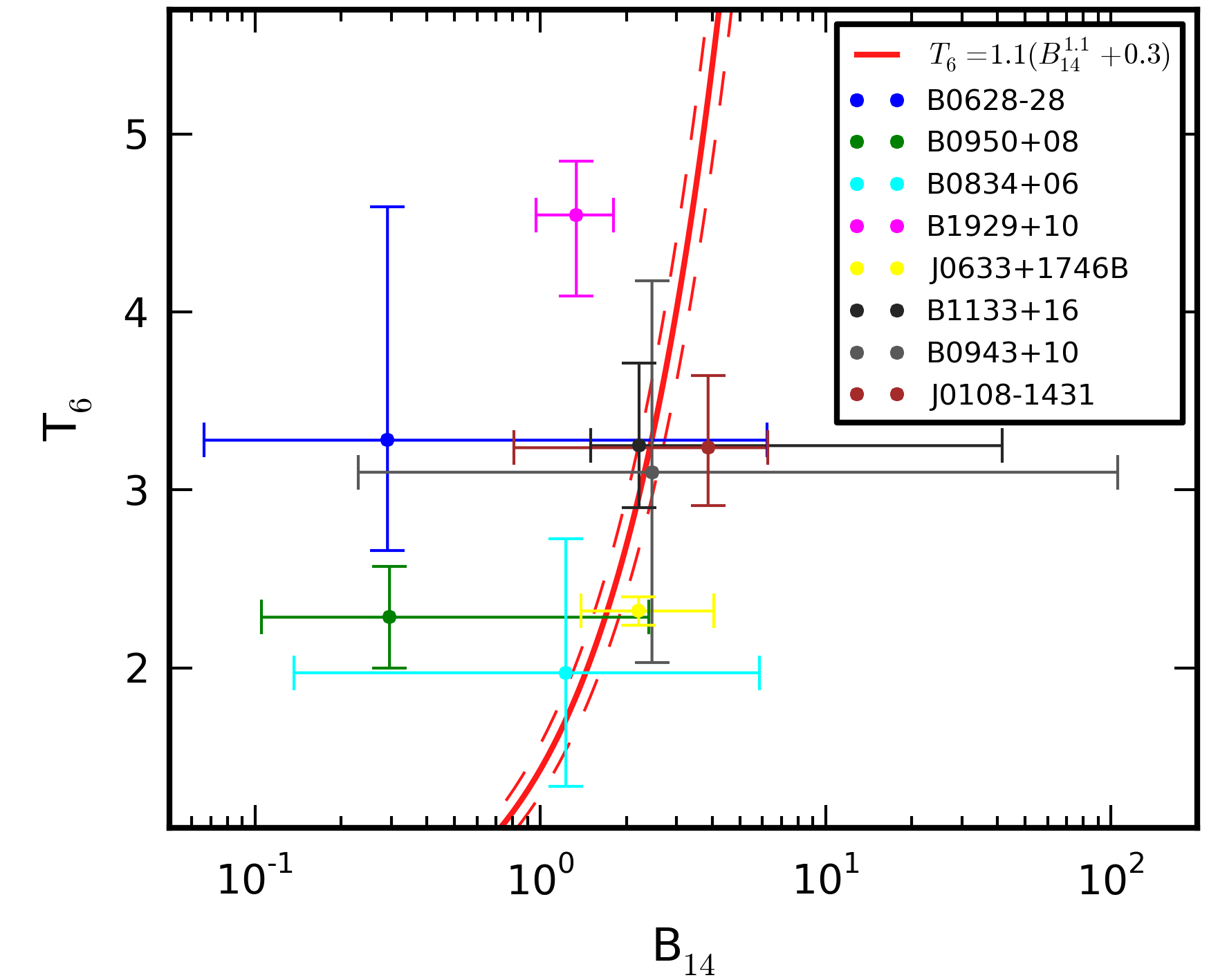
Figure 2: Diagram of the surface temperature ($T_{6}=T_{s}/10^{6}$) vs. the surface magnetic field ($B_{14}=B_{s}/10^{14}$). The red line is the critical temperature ($T_{\rm crit}$) evaluated from [4] and dashed lines corresponds to uncertainties in calculations. Left panel includes all pulsars with $b>1$ while right panel is zoom of the upper right part of the graph. Error bars corresponds to $1\sigma$.

According to our model the actual surface temperature equals to the critical value ($T_{s}\sim T_{\rm crit}$) which leads to the formation of Partially Screened Gap (PSG) above the polar caps of neutron star [5]. Hot spot parameters derived from X-ray observations of isolated neutron stars are presented in Table 1.

2 The Model

The PSG model assumes existence of heavy (Fe⁵⁶) ions with density near but still below corotational charge density ($\rho_{\rm GJ}$), thus the actual charge density causes partial screening of the potential drop just above the polar cap. The degree of shielding can be described by parameter $\eta=1-\rho_{i}/\rho_{\rm GJ}$ where $\rho_{i}$ is the charge density of heavy ions in the gap. The thermal ejection of ions from surface causes partial screening of the acceleration potential drop

$$\Delta V=\eta\Delta V_{max}=2\pi\eta B_{s}h^{2}/cP,$$ (1)

where $\Delta V_{max}$ is the potential drop in vacuum gap, $h$ is the gap height, $B_{s}=bB_{d}$ surface magnetic field (applicable only if $b>1$). Using calculations of Medin & Lai [4] we can express the dependence of the critical temperature on pulsar parameters as

$$T_{\rm crit}=1.6\times 10^{4}\left(\left(\left(P\dot{P}_{-15}\right)^{0.5}b\right)^{1.1}+17.7\right)$$ (2)

or $T_{\rm crit}=1.1\times 10^{6}\left(B_{14}^{1.1}+0.3\right)$, where $B_{14}=B_{s}/10^{14}$.

The actual potential drop $\Delta V$ should be thermostatically regulated and there should be established a quasi-equilibrium state, in which heating due to electron/positron bombardment is balanced by cooling due to thermal radiation (see [5] for more details). The necessary condition for formation of this quasi-equilibrium state is

$$\sigma T_{s}^{4}=\eta e\Delta Vcn_{\rm GJ},$$ (3)

where $\sigma$ is the Stefan-Boltzmann constant, $e$ - the electron charge, $n_{\rm GJ}=\rho_{\rm GJ}/e=1.4\times 10^{11}b\dot{P}_{-15}^{0.5}P^{-0.5}$ is the corotational number density. Using equations (2) and (3) we can express the acceleration potential drop as

$$\Delta V=7.3\times 10^{5}\eta^{-1}B_{14}^{-1}\left(B_{14}^{1.1}+0.3\right)^{4}P,$$ (4)

and finally using equations (1) and (4) we can estimate the gap height in PSG model as

$$h\eta=6B_{14}^{-1}\left(B_{14}^{1.1}+0.3\right)^{2}P$$ (5)

As we see both $\Delta V$ and $h$ depend on shielding factor $\eta$ which actually depends on the details of the avalanche pair production in the gap. First we need to determine which process, Curvature Radiation (CR) or Inverse Compton Scattering (ICS), is responsible for the pair production. We will need following parameters: $l_{\rm acc}$ - the distance which a particle should pass to gain Lorentz factor equal to $\gamma_{\rm acc}$, $l_{e}$ - the mean length an electron (or positron) travels before a gamma-photon is emitted, and $l_{\rm ph}$ - the mean free path of gamma-photon before being absorbed by the magnetic field.

2.1 Acceleration path

In the frame of PSG model, using formalism described in [6], we estimate the component of electric field along the magnetic field line in the gap as

$$E\approx\eta\frac{4\pi B_{s}}{cP}(h-z)$$ (6)

which vanishes at the top $z=h$. The Lorentz factor of particles after distance $l_{\rm acc}$ can be calculated as follows

$$\gamma_{\rm acc}=\frac{e}{m_{e}c^{2}}\int_{z_{1}}^{z_{2}}Edz\approx\eta\frac{4\pi B_{s}e}{m_{e}c^{3}P}(z_{2}-z_{1})(h-\frac{z_{1}+z_{2}}{2})$$ (7)

where $m_{e}$ is mass of an electron and $z_{2}-z_{1}=l_{\rm acc}$. Then we can approximate $z_{1}+z_{2}\approx 2z$ and assume $z\approx h/2$, thus

$$l_{\rm acc}=\gamma_{\rm acc}\frac{m_{e}c^{3}P}{2\pi h\eta B_{s}e}.$$ (8)

2.2 Electron or positron mean free paths

The mean free path of electron or positron ($l_{e}$) can be defined as the mean length that a particle passes until a gamma-photon is emitted. In the case of CR electron mean free path can be estimated as a distance that particle with Lorentz factor $\gamma$ travels during the time which is necessary to emit curvature photon (see [7])

$$l_{e,cr}\sim c\left(\frac{P_{cr}}{E_{\gamma,cr}}\right)^{-1}=\frac{9}{4}\frac{\hbar\Re c}{\gamma e^{2}},$$ (9)

where $P_{cr}=2\gamma^{4}e^{2}c/3\Re^{2}$ is the power of the CR, $E_{\gamma,cr}=3\hbar\gamma^{3}c/2\Re$ is the characteristic photon energy, $\Re$ - the curvature radius of magnetic field lines.

For the ICS process, calculation of the electron mean free path $l_{e,ics}$, is not as simple as that of the CR process. Although we can define $l_{e,ics}$ in a same way as we defined $l_{e,cr}$ but it is difficult to estimate a characteristic frequency of emitted photons. We have to take into account photons of various frequencies with various incident angles. An estimation of the mean free path of electron (or positron) to produce a photon is [8]

$$l_{e,ics}\sim\left[\int_{\mu_{0}}^{\mu_{1}}\int_{0}^{\infty}{\sigma^{\prime}(\epsilon,\mu_{i})(1-\beta\mu_{i})n_{\rm ph}(\epsilon)d\epsilon d\mu_{i}}\right]^{-1}$$ (10)

where $\epsilon$ is the incident photon energy in units of $m_{e}c^{2}$, $\mu_{i}=\cos{\psi_{i}}$ is the cosine of the photon incident angle, $\beta=v/c$ is the velocity in terms of speed of light,

$$n_{\rm ph}=\frac{4\pi}{\lambda_{c}^{3}}\frac{\epsilon^{2}}{\exp{(\epsilon/\theta)}-1}d\epsilon$$ (11)

represents the photon number density distribution of a semi-isotropic blackbody radiation, $\theta=kT_{s}/m_{e}c^{2}$, $k$ is the Boltzmann constant, and $\lambda_{c}=h/m_{e}c=2.424\times 10^{-10}$ cm is the electron Compton wavelength. Here $\sigma^{\prime}$ is the cross section of scattering in the particle rest frame. In the Thomson regime cross section of scattering in the particle rest frame can be written as [9]

$$\sigma^{\prime}=\frac{\sigma_{T}}{2}\left[\frac{u^{2}}{(u+1)^{2}}+\frac{u^{2}}{(u-1)^{2}+a^{2}}\right],$$ (12)

where $\sigma_{T}$ is the Thomson cross section, $u=\epsilon^{\prime}/\epsilon_{B}$, $a=\frac{2}{3}\alpha_{f}\epsilon_{B}$, $\epsilon^{\prime}=\gamma\epsilon(1-\beta\mu_{i})$ is the incident photon energy in the particle rest frame in units of $m_{e}c^{2}$, $\epsilon_{B}=B_{s}/B_{q}$ is the electron cyclotron resonance energy in units of $m_{e}c^{2}$, $B_{q}=m_{e}^{2}c^{3}/e\hbar=4.413\times 10^{13}$ G, and $\alpha_{f}=e^{2}/\hbar c$ is the fine-structure constant.

Equation (12) however does not include the quantum relativistic effects of a strong magnetic field ($B_{s}>0.1B_{q}$), therefore, it can be used only at altitudes where magnetic field is relatively weaker. For strong magnetic fields we can use an approximation proposed in [10] and then an approximate averaged (polarization-independent) cross section can be written as follows

$$\sigma^{\prime}=\frac{3\sigma_{T}}{8}\frac{\epsilon\epsilon^{\prime 2}(1+\mu_{i}^{2})}{2\epsilon-\epsilon^{\prime}}\left[\frac{1}{(\epsilon-\beta_{q})^{2}}+\frac{1}{(\epsilon+\beta_{q})^{2}}\right],$$ (13)

where $\beta_{q}=B_{s}/B_{q}$. Equation (13) represents the exact cross section when the particle after scattering falls on the zero Landau state (see [10] for more accurate results).

We should expect two modes of ICS process, resonant and non-resonant. The resonant ICS takes place if the photon frequency in particle rest frame equals to the cyclotron electron frequency. Non-resonant ICS includes all scattering processes of photons with frequencies around the maximum of the thermal spectrum. At resonance frequency equation (13) has a singularity, so it could be used only for non-resonant case. For resonant case, one should use approach proposed in [11], thus the cross section in the particle rest frame is

$$\sigma_{res}^{\prime}\simeq 2\pi^{2}\frac{e^{2}\hbar}{m_{e}c}\delta(\epsilon^{\prime}-\epsilon_{b})$$ (14)

Equation (14) can be also used for strong magnetic fields ($\beta_{q}>0.1$), since the resonant condition $\epsilon^{\prime}=\epsilon_{b}$ holds regardless of field strength. Although one have to remember that this equation represents the upper limit for cases with very high magnetic fields (see [10] for more details). The particle mean free path above a polar cap for the resonant ICS process is

$$l_{e,rics}\sim\left[\int_{\mu_{0}}^{\mu_{1}}\int_{0}^{\infty}{\sigma_{res}^{\prime}(1-\beta\mu_{i})n_{\rm ph}(\epsilon)d\epsilon d\mu_{i}}\right]^{-1}=\left[\frac{2\pi e^{2}\hbar}{m_{e}c\gamma}\int_{\mu_{0}}^{\mu_{1}}n_{\rm ph}\left(\frac{\epsilon_{b}}{1-\beta\mu_{i}}\right)d\mu_{i}\right]^{-1}$$ (15)

For the altitudes of the same order as the polar cap size we can use $\mu_{0}=1$, $\mu_{1}=0$ as incident angle limits for outflowing particles, and $\mu_{0}=0$, $\mu_{1}=-1$ as incident angle limits for backflowing particles.

2.3 Photon mean free path

A photon with energy $E_{\gamma}>2m_{e}c^{2}$ and propagating with nonzero angle $\psi$ with respect to an external magnetic field can be absorbed by the field and as a result electron-positron pair is created. The optical depth of a such process can be defined as [11]

$$\tau=s_{\rm ph}R_{\|,\perp},$$ (16)

where $s_{\rm ph}$ is a distance traveled by an photon, $R_{\|,\perp}=R^{\prime}_{\|,\perp}\sin{\psi}$ is the attenuation coefficient for the $\|$ or $\perp$ polarized photons, and $R^{\prime}$ is the attenuation coefficient in the ”perpendicular” frame (the frame where the photon propagates perpendicular to the local magnetic field).

The total attenuation coefficient for pair production is given by $R^{\prime}=\sum_{jk}R^{\prime}_{j,k}$, where $R^{\prime}_{j,k}$ is the attenuation coefficient for process (channel) in which the photon produces an electron in Landau level $j$ and positron in Landau level $k$, and the sum is taken over all possible states for the electron-positron pair. Since pair production is symmetric with respect to the electron and positron, $R^{\prime}_{kj}=R^{\prime}_{kj}$ for simplicity we will use $R^{\prime}_{jk}$ to represent the combined probability of creating the pair in either $(jk)$ or $(kj)$ state. For a given channel $(jk)$, the threshold condition for pair production is:

$$E_{\gamma}^{\prime}>E_{j}^{\prime}+E_{k}^{\prime},$$ (17)

where $E_{\gamma}^{\prime}=E_{\gamma}\sin{\psi}$ is the photon energy in the perpendicular frame and $E_{n}^{\prime}=m_{e}c^{2}\sqrt{1+2\beta_{q}n}$ is the minimum energy of an electron/positron in Landau Level $n$. In dimensionless form this condition can be written as

$$x=\frac{E_{\gamma}^{\prime}}{2mc^{2}}=\frac{E_{\gamma}}{2m_{e}c^{2}}\sin{\psi}>\frac{1}{2}\left[\sqrt{1+2\beta_{q}j}+\sqrt{1+2\beta_{q}k}\right]$$ (18)

The first nonzero attenuation coefficients for both polarizations are given in [12]:

$$R^{\prime}_{\|,00}=\frac{1}{2a_{0}}\frac{\beta_{q}}{x^{2}\sqrt{x^{2}-1}}e^{-2x^{2}/\beta_{q}},\hskip 28.45274ptx>x_{1}=1;$$ (19)

$$R^{\prime}_{\perp,01}=2\times\frac{1}{2a_{0}}\frac{\beta_{q}}{2x^{2}}\frac{2x^{2}-\beta_{q}}{\sqrt{x^{2}-1-\beta_{q}+\frac{\beta_{q}^{2}}{4x^{2}}}}e^{-2x^{2}/\beta_{q}},\hskip 28.45274ptx>x_{2}=\left(1+\sqrt{1+2\beta_{q}}\right)/2;$$ (20)

where $a_{0}$ is Bohr radius (let us note that $R^{\prime}_{\perp,00}=0$ and higher orders of attenuation coefficients should be used if $x>x_{3}=\left(1+\sqrt{1+4\beta_{q}}\right)/2$).

The optical depth is defined as:

$$\tau=\int_{0}^{s_{\rm ph}}R(s)ds=\int_{0}^{s_{\rm ph}}R^{\prime}(s)\sin{\psi}ds$$ (21)

We can assume $\psi\ll 1$, because all high energy photons ($x>1$) will produce pairs much earlier then $\psi$ reaches value near unity. In this limit $\sin{\psi}\simeq s_{\rm ph}/\Re$ so relation between $x$ and $s_{\rm ph}$ can be expressed by

$$x\simeq\frac{s_{\rm ph}}{\Re}\frac{E_{\gamma}}{2m_{e}c^{2}}.$$ (22)

The equation (21) can be rewritten as

$$\tau=\tau_{1}+\tau_{\|,2}+\tau_{\perp,2}+...$$

$$\tau_{1}=\int_{s_{1}}^{s_{2}}R_{\|,00}ds,\hskip 14.22636pt\tau_{\|,2}=\int_{s_{2}}^{s_{3}}\left(R_{\|,00}+R_{\|,01}\right)ds,\hskip 14.22636pt\tau_{\perp,2}=\int_{s_{2}}^{s_{3}}R_{\perp,01}ds$$ (23)

where $s_{1}$ and $s_{2}$ are distances which the photon should pass in order to have energy $x_{1}$ and $x_{2}$ respectively (in perpendicular frame of reference). Let us note that $s_{1}$, $s_{2}$, and $s_{3}$ are of the same order and if $s<s_{1}$ attenuation coefficient is zero. As shown in [11] for strong magnetic fields ($\beta_{q}\gtrsim 0.1$) $\tau_{1}$, $\tau_{\|,2}$, and $\tau_{\perp,2}$ are much larger then one. Therefore, the pair production process happens according two scenarios. If $\beta_{q}\gtrsim 0.1$ photons produce pairs almost immediately upon reaching the first threshold, so the created pairs will be in low Landau levels ($n\lesssim 2$). If $\beta_{q}\lesssim 0.1$ photons will travel longer distances to be absorbed and created pairs will be in higher Landau levels.

Thus, for strong magnetic fields ($\beta_{q}\gtrsim 0.1$) electron mean free path can be calculated as

$$l_{\rm ph}\sim s_{1}=\Re\frac{2m_{e}c^{2}}{E_{\gamma}},$$ (24)

and for relatively weak magnetic fields ($\beta_{q}\lesssim 0.1$) we can use asymptotic approximation derived by Erber [13]

$$l_{\rm ph}=\frac{4.4}{(e^{2}/\hbar c)}\frac{\hbar}{m_{e}c}\frac{1}{\beta_{q}\sin{\psi}}\exp{\left(\frac{4}{3x\beta_{q}}\right)}$$ (25)

2.4 Partially Screened Gap height

As we mentioned above, PSG can exist if equation (3) is satisfied. On the other hand for the heating of the stellar surface the high enough flux of back-streaming particles is required. Thus, we need to estimate shielding factor $\eta$ and gap height $h$ which are the main parameters of PSG. Let us note that $\eta$ and $h$ are connected with each other by equation (5). Generally gap height can by defined as $h\approx l_{e}+l_{ph}$ with the necessary condition that $l_{e}>l_{acc}$. Latter corresponds to demand that the particle should gain the energy that is required for photon emission by either ICS or CR processes. The Fig. 3 shows dependence of free paths on the particles Lorentz factor $\gamma$ for some particular pulsar parameters (dependence on pulsar parameters will be discussed in section 3). Let us note that this free paths do not depend on the gap height $h$ (see equations (9), (15), (24)). As it follows from equation (8) $l_{acc}$ also does not depend on a gap height because $h$ and $\eta$ are connected by equation (5).

Results presented in the Fig. 3 do not allow us to define the gap height unambiguously but we can already find that CR is the dominant pair creation process for PSG scenario. Although $l_{e,ics}<l_{e,cr}$ for particles with $\gamma\sim 10^{3}-10^{4}$ the gamma-photon production by ICS process is not effective because $l_{\rm acc}<<l_{e,ics}$, i.e. the particles will be accelerated to higher energies ($\gamma\sim 10^{5}-10^{6}$) before they would upscatter X-ray photons emitted from the hot polar cap.

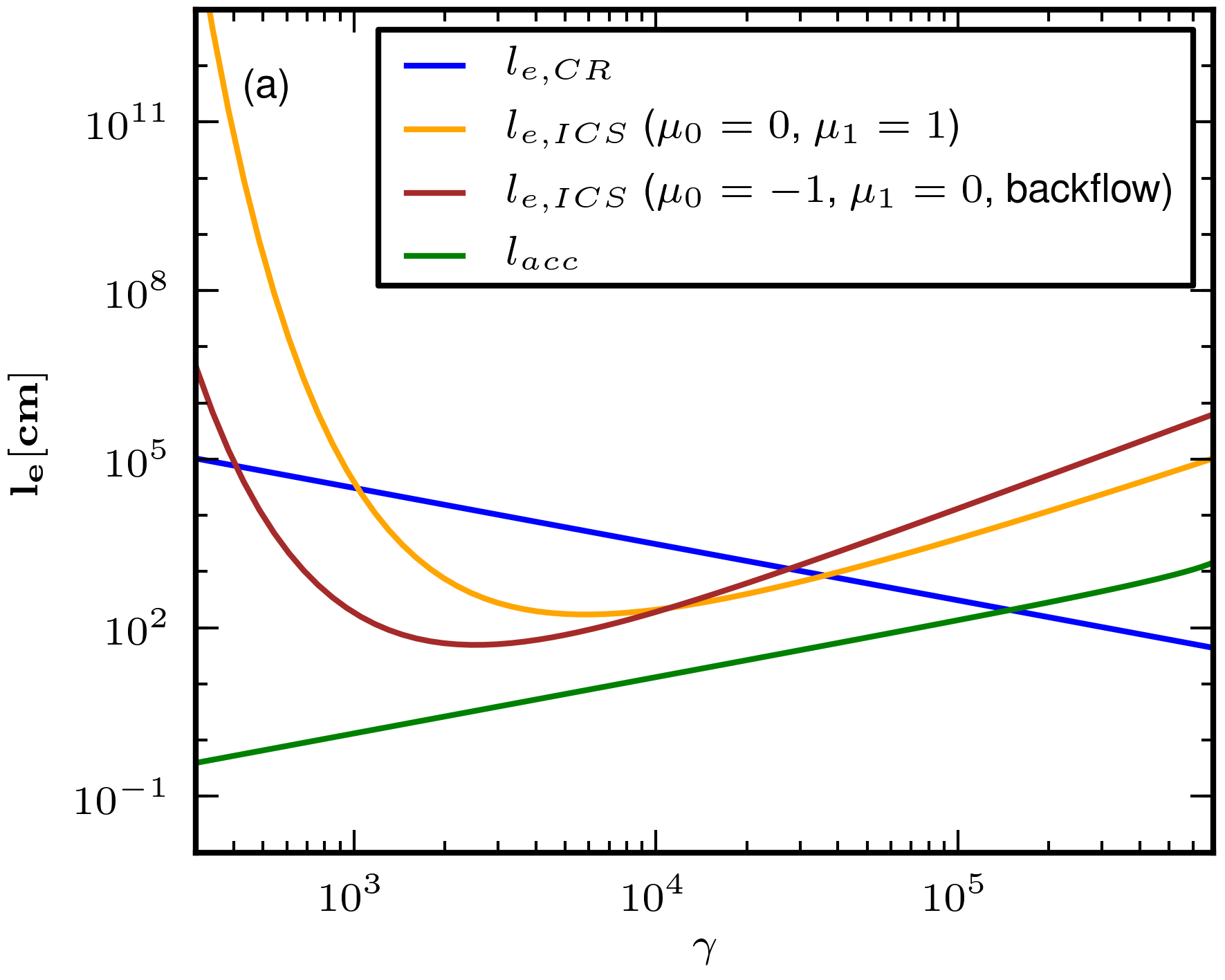
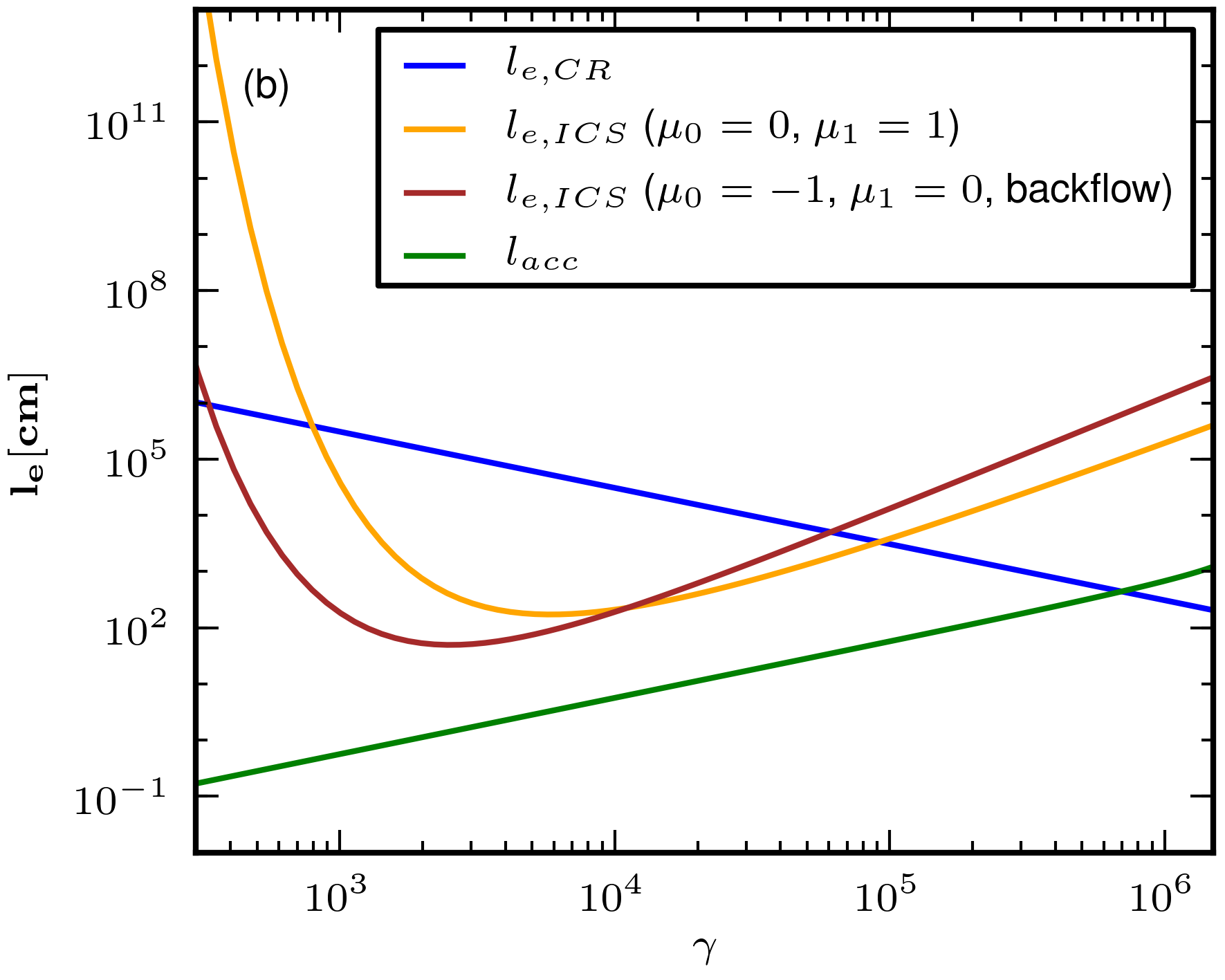
Figure 3: Diagram of the electron/positron mean free path for both CR and ICS processes. The left panel (a) corresponds to calculations for $B_{14}=1.5$, $T_{6}=1.9$, $\Re_{6}=0.1$, $P=1$ while the right panel (b) corresponds to calculations for $B_{14}=3.5$, $T_{6}=4.4$, $\Re_{6}=1$, $P=1$. Acceleration path was calculated for the same gap parameters ($h=20$ m, $\eta=0.03$) in both panels (see discussion in section 2.4). Although $l_{e,ics}<l_{e,cr}$ for particles with $\gamma\sim 10^{3}-10^{4}$ the $\gamma$-photon production by ICS process is not effective because for these particle $l_{\rm acc}<<l_{e,ics}$. That means that they will be accelerated to higher energies ($\gamma\sim 10^{5}-10^{6}$) before they would upscatter X-ray photons emitted from the stellar surface.

As soon as we determine the dominant process, i.e. CR, which is responsible for gamma-photons emission we can estimate the gap height. Curvature emission by a particle is effective for Lorentz factors $\gamma\sim 10^{5}-10^{6}$ (when $l_{e,cr}\leq l_{\rm acc}$). The reaction force although is not high enough to stop the acceleration by electric field. Equilibrium between acceleration and deceleration (by reaction force) would be established when the CR power would equal to ”electric power” ($P_{cr}=P_{\rm acc}$, where $P_{\rm acc}=4\pi\eta vB_{s}(h-z)/cP$ is work done by electric field in unit of time). Using the characteristic Lorentz factors of radiating particles we can find characteristic frequencies of CR photons and thus, we can check whether the necessary condition ($l_{e}+l_{\rm ph}\leq h$) for cascade formation is satisfied.

The Fig. 4 shows dependence of the CR photon mean free path ($l_{ph}$), the particle mean free path ($l_{e}$), and the acceleration path ($l_{acc}$) on the energy expressed in units of $m_{e}c^{2}$. Top axis shows the Lorentz factors of particles which emit the curvature photons with energy shown on bottom axis. While the energy of particle falls in blue region in the Fig. 4 there will be no CR because the particle will be accelerated to higher energies before it travels distance enough to emit one curvature photon ($l_{e}>l_{\rm acc}$). For the energies in green region CR is most efficient. The particle in the PSG never can reach energies falling in red region because reaction force caused by CR process is bigger then acceleration force. Thus, the characteristic Lorentz factor $\gamma_{c}$ of particles (and characteristic photon energy $E_{c}$) corresponds to value defined by the border between green and red region. Therefore, we can define gap height for the characteristic energies $\gamma_{c}$ and $E_{c}$ as

$$l_{e}(\gamma=\gamma_{c})+l_{ph}(E_{\gamma}=E_{c})<h$$ (26)

Then we have to calculate $l_{e}$, $l_{ph}$ for different values of $h$ and check which value satisfies condition (26). The Fig. 4 shows two cases: panel (a) that corresponds to $h=10$ m and panel (b) which corresponds to $h=40$ m. From panel (a) we can see that condition (26) is not satisfied while for gap height $h=40$ m cascade process will form. This approach allows us to calculate minimum height at which gap sparking breakdown is possible and thus, we can estimate unambiguously the gap height in the frame of the PSG model.

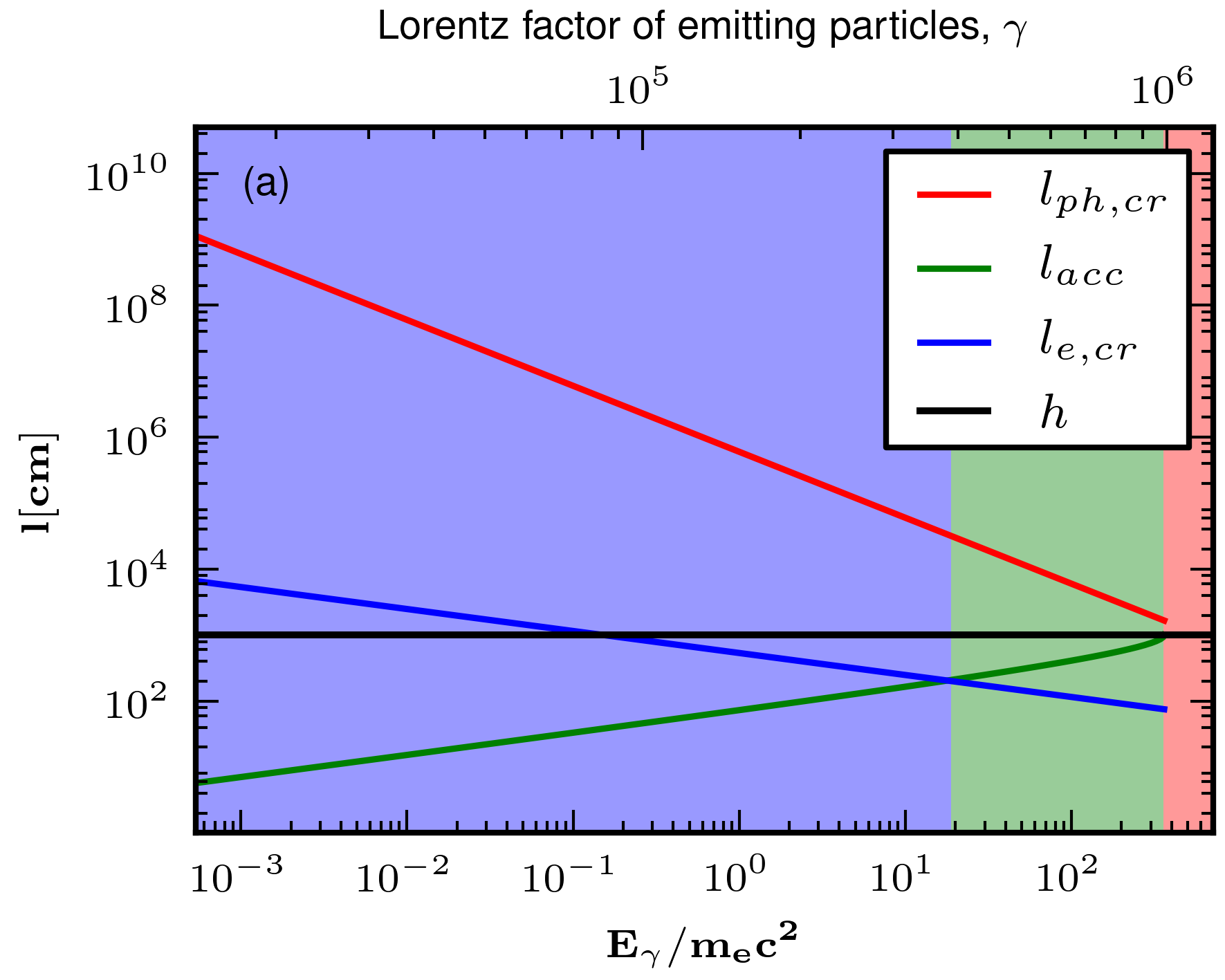
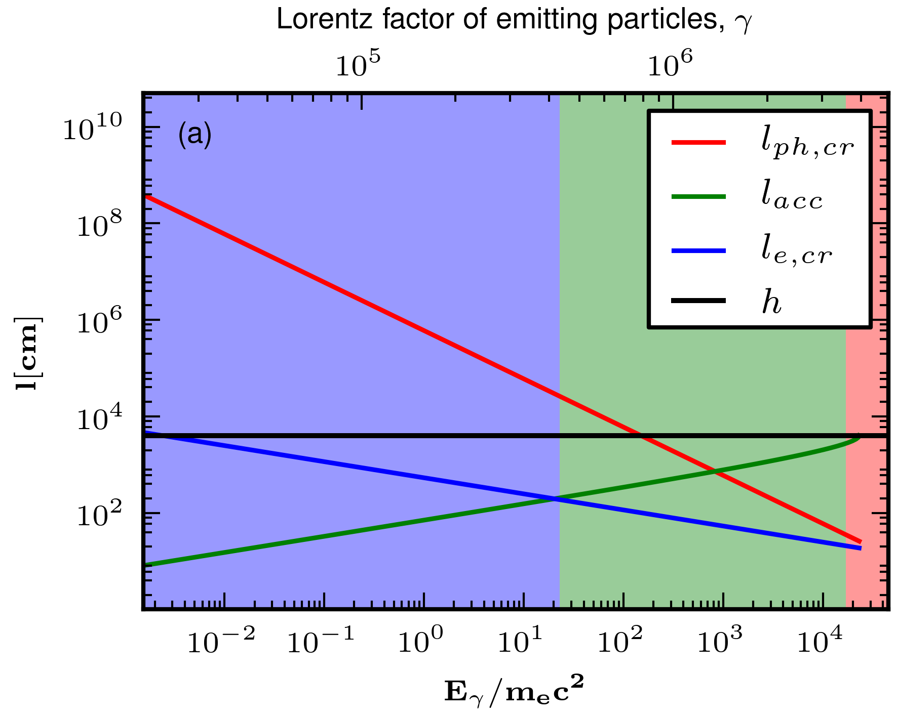
Figure 4: Diagram of the photon mean free path, the particle mean free path, and the acceleration path vs. the photon energy and the Lorentz factor of accelerated particles (top axis) for specific pulsar ($B_{14}=3.5$, $T_{6}=4.39$, $\Re_{6}=0.3$, $P=1$). See description of blue, green and red regions in the text above equation (26). The black horizontal line corresponds to the gap height. Calculations for panel (a) were done using $h=10$ m, $\eta=0.03$ while for panel (b) using $h=40$ m, $\eta=0.01$.

3 Observational consequences

In order to compare the model with observations we need to define main parameters of PSG model for a given pulsar with known period and period derivative.

3.1 PSG model parameters

We can distinguish two types of PSG parameters: observed and derived. As we mention above in some cases when X-ray observations are available we can directly estimate surface magnetic filed $B_{s}$. On one hand $B_{s}$ can be calculated using the size of the hot spot $A_{\rm BB}$, and on the other hand we can find $B_{s}$ using estimation of the critical temperature and assumption that $T_{s}=T_{\rm crit}$. One of the most important requirements of PSG model is that these two estimations should coincide with each others. As it is clear from Fig. 2 in most cases when the hot spot parameters are available this requirement is fulfilled. Thus, we can assume the characteristic values of $B_{s}$ vary in range of $(1-4)\times 10^{14}$ which corresponds to critical/surface temperature in range of $(1.1-4.5)\times 10^{6}$ (see Table 1). Using these values we can estimate derived parameters of PSG such us the gap height $h$, the shielding factor $\eta$ and the Lorentz factor of primary particles $\gamma_{c}$. Let us note that these parameters depend also on the curvature radius of magnetic field lines $\Re$. The curvature can not be neither observed or derived but modeling of surface magnetic field (see Fig. 1) indicates that the curvature radius varies in the range of $(0.1-1)\times 10^{6}$ cm. Below we will discuss influence of pulsar parameters such as the magnetic field, the curvature of field lines and the period on derived PSG parameters.

3.2 Influence of the magnetic field

The conditions in PSG are mainly defined by the surface magnetic field. In Fig. 5 panel (a) we present dependence of the gap height on the surface magnetic field calculated according to approach described in section 2.4. It is clear that the gap height decreases as the surface magnetic field increases. The Fig. 5 panel (b) shows dependence of the shielding factor on the surface magnetic field calculated using equation (5). We can see that for stronger magnetic fields $\eta$ increases which means that the density of heavy ions above the polar cap decreases. Let us note that the surface temperature ($T_{s}$) stays very near to the critical temperature ($T_{\rm crit}$) which is shown on the top axis of the diagrams. In Fig. 5 panel (c) we present dependence of Lorenz factors of the particles accelerated in PSG. The Green line ($\gamma_{0}$) presents the values corresponding to the boundary between blue and green region in the Fig. 4 while the red line corresponds to the boundary between the green and the red region which is the characteristic value ($\gamma_{c}$) for primary particles. We see that $\gamma_{c}$ is very slightly affected by the magnetic field strength.

One can expect that for higher temperatures (which correspond to stronger magnetic fields) the gap breakdown could be dominated by ICS process. However this is not the case because the particle mean free path is much higher then the acceleration path ($l_{e,ics}>>l_{\rm acc}$) even for strong magnetic fields.

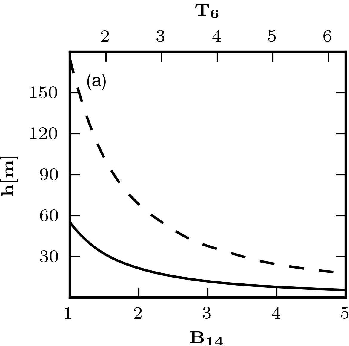
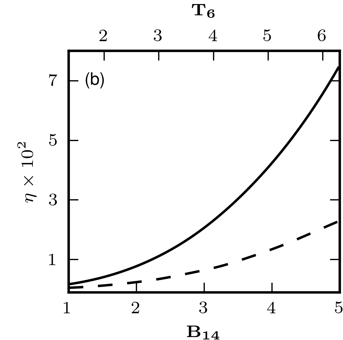
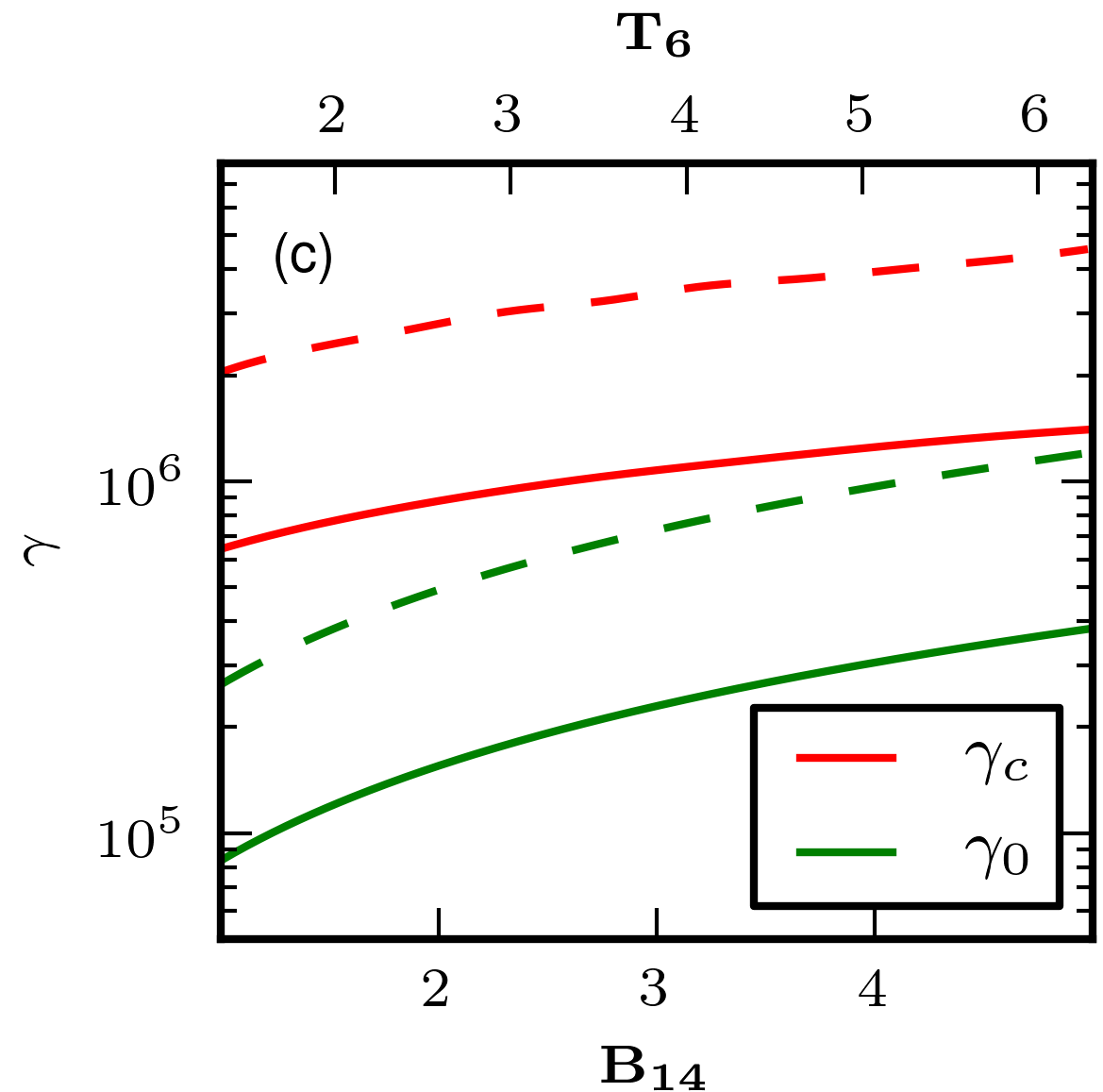
Figure 5: Dependence of the gap height (panel a), the shielding factor (panel b), and the particles Lorentz factor (panel c) on the surface magnetic field. Solid lines correspond to calculations for $\Re_{6}=0.1$ while dashed lines correspond to calculations for $\Re_{6}=1$. For both cases the pulsar period $P=1$ was used. The green line presents the values corresponding to the boundary between blue and green region in the Fig. 4 while the red line corresponds to the boundary between green and red region. Corresponding critical temperature is shown on top axis of diagrams.

3.3 Influence of the field lines curvature radius

The curvature of magnetic field lines significantly affects the PSG parameters since the CR process is responsible for PSG breakdown. As it can be expected the gap height decreases for smaller curvature radius of magnetic field lines (Fig. 6 panel a) since CR is more efficient for smaller values of the curvature radius. Consequently the shielding factor decreases with increasing curvature radius of magnetic field lines (Fig. 6 panel b).

The Lorentz factor of primary particles increases for bigger radius of curvature (Fig. 6 panel c), since both conditions $l_{e}\sim l_{\rm acc}$ and $P_{cr}\sim P_{\rm acc}$ are satisfied for higher Lorentz factors.

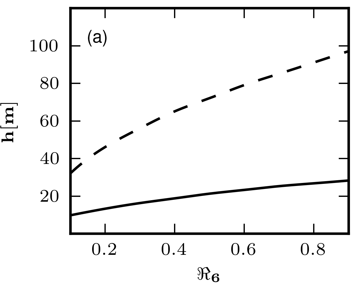
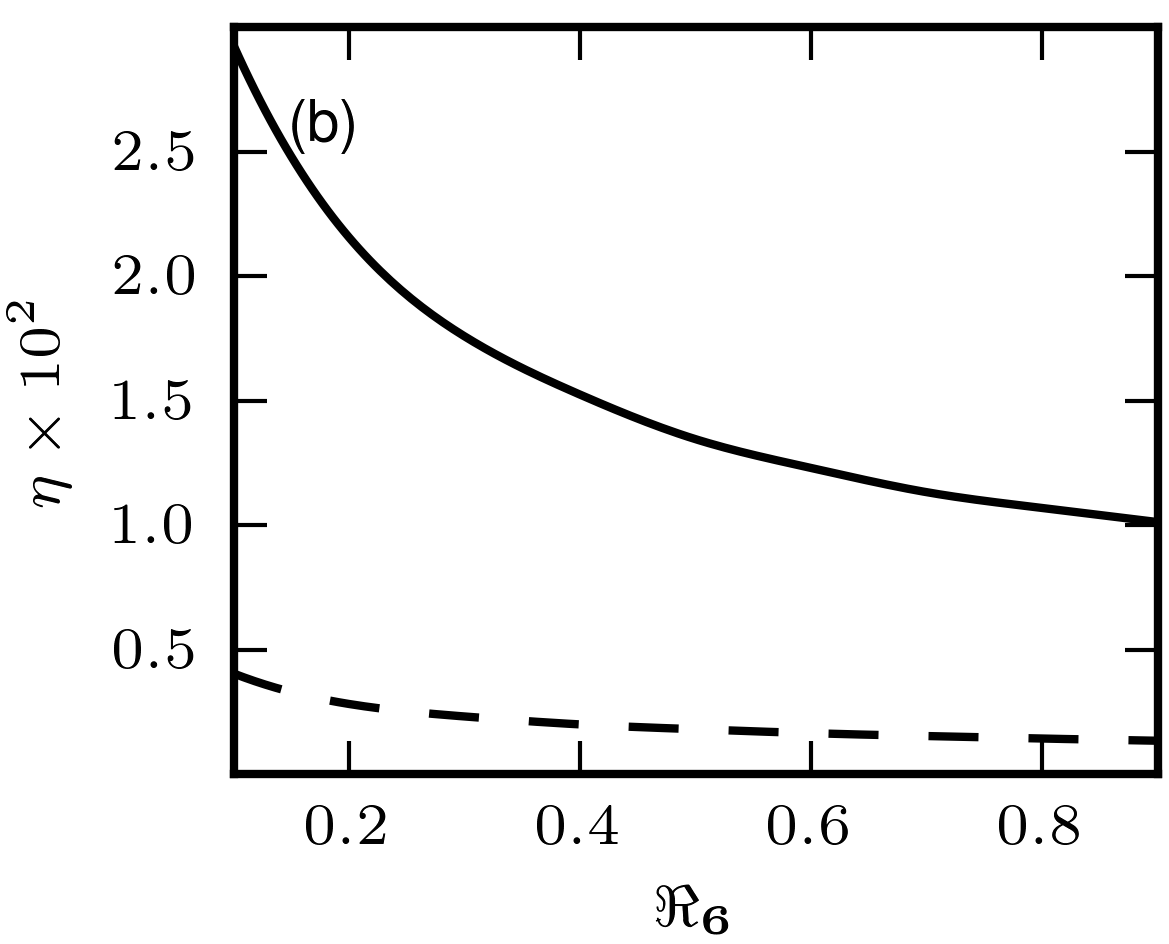
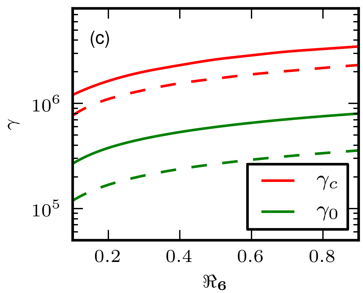
Figure 6: Dependence of the gap height (panel a), the shielding factor (panel b), and the particles Lorentz factor (panel c) on the curvature radius of magnetic field lines. Solid lines correspond to calculations for $B_{14}=3.5$ while dashed lines correspond to calculations for $B_{14}=1.5$. For both cases the pulsar period $P=1$ was used.

3.4 Influence of the pulsar period

As we can see from figure 7 panel (a) and panel (c) neither the gap height nor the Lorentz factor of primary particles depend on pulsar period. This is one of the most important result of our calculations. The shielding factor is just proportional to period (Fig. 7 panel b) as is expected from equation (5).

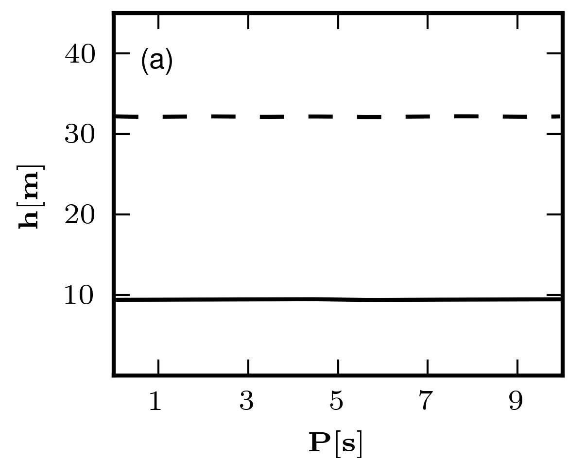
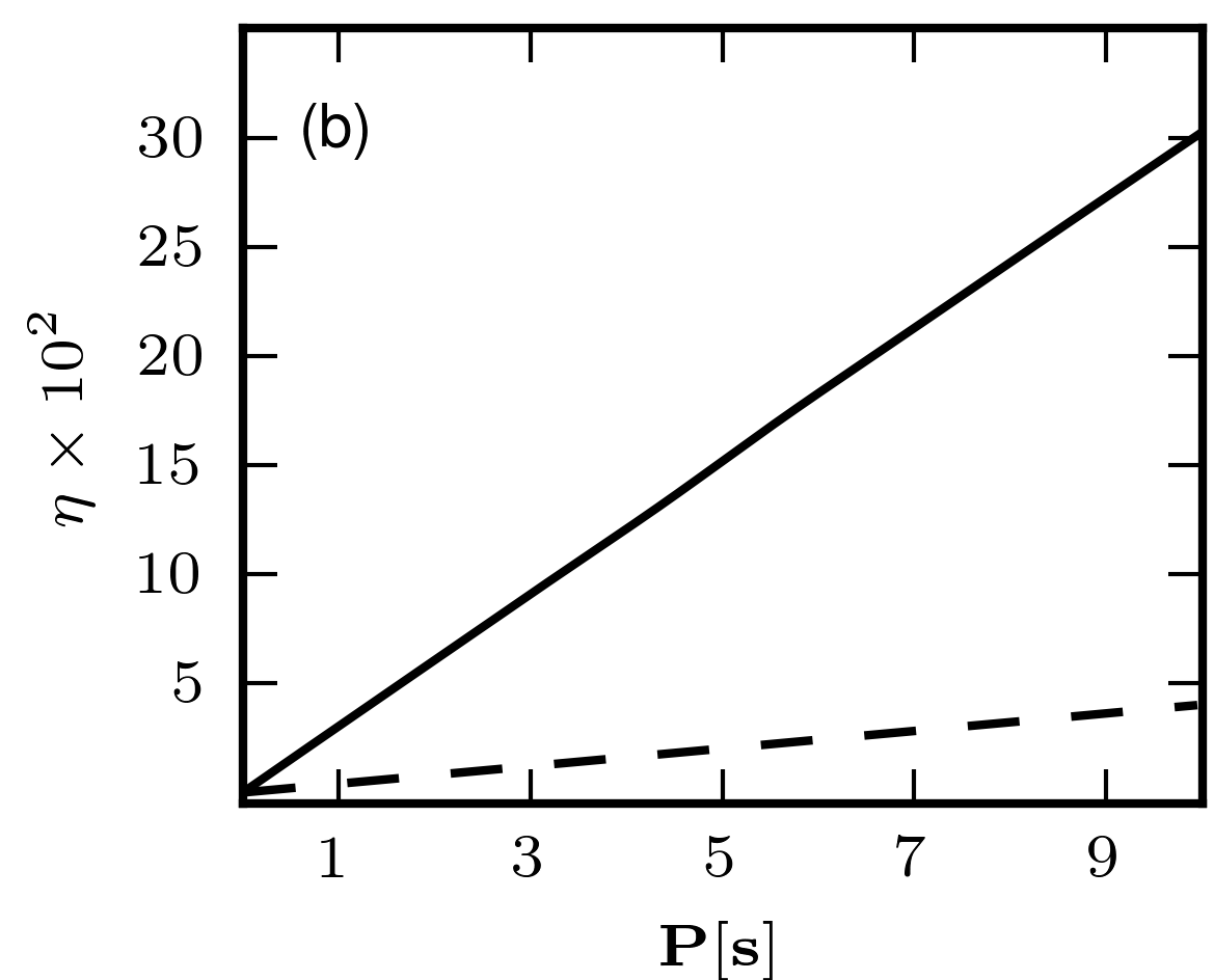
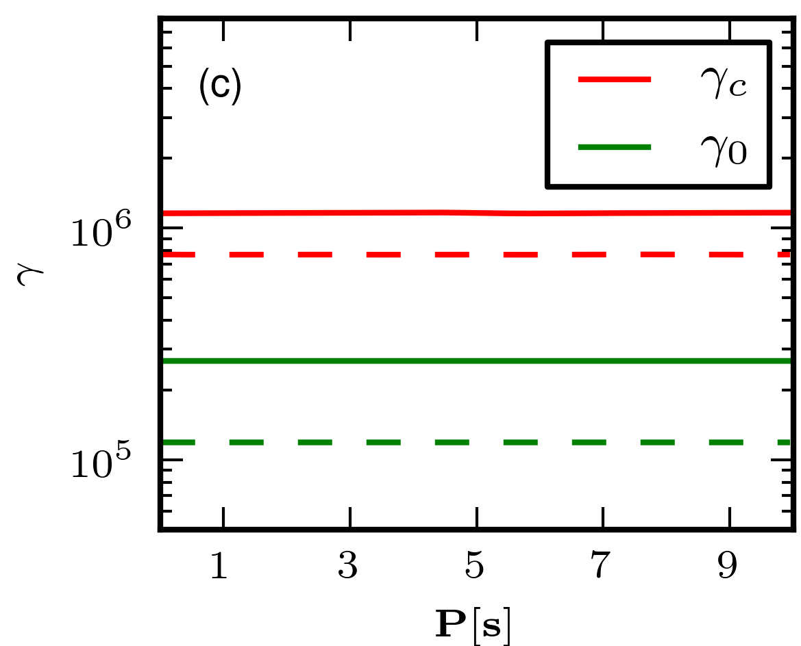
Figure 7: Dependence of the gap height (panel a), the shielding factor (panel b), and the particles Lorentz factor (panel c) on the pulsar period. Solid lines correspond to calculations for $B_{14}=3.5$ while dashed lines correspond to calculations for $B_{14}=1.5$. For both cases the radius of curvature $\Re_{6}=0.1$ was used.

4 Conclusions

X-ray observations of pulsars show that temperature of the hot spot is about few million kelvins while its area is much smaller then the conventional polar cap surface which is calculated assuming purely dipolar geometry of pulsar magnetic field. Such observations can be easily explained in the frame of PSG model which assumes that the geometry of magnetic field near the stellar surface differs significantly from dipolar one, actually the field is much stronger and curved. At the same time the surface temperature is about the critical temperature which depends only on the magnetic field strength.

In this paper we calculated dependence of the gap parameters such as the gap height, the shielding factor, and characteristic energies of primary particles on the surface magnetic field, the curvature radius of field lines, and the pulsar period in the frame of PSG model. The surface magnetic field can be calculated using the X-ray observations (if such data are available), however the curvature radius can be only estimated by simulations of different geometry of magnetic field lines. Let us note that the gap height is the most important parameter for all models of the Inner Acceleration Region in pulsars. We can define the gap height as a sum of the particle mean free path and the photon mean free path, $h\approx l_{e}+l_{ph}$. In order to estimate the PSG height we discuss two processes responsible for cascade pair production: the Inverse Compton Scattering and the Curvature Radiation. We found that CR is the dominant process for the sparking breakdown of the PSG. Although ICS is more efficient for particles with $\gamma\sim 10^{3}-10^{4}$, the particles are accelerated to higher energies $\gamma\sim 10^{5}-10^{6}$ before they upscatter X-ray photons emitted from the polar cap. As soon as particles Lorentz factor $\gamma>10^{5}$ CR is more efficient then ICS. In section 3 we show the dependence of PSG parameters ($h$, $\eta$, $\gamma_{c}$) on the pulsar parameters ($B_{s}$, $\Re$, $P$). Since CR is the dominant process for gamma-photon emission the PSG parameters strongly depend on curvature radius of magnetic field lines. Pulsars with smaller curvature radius should have the lower gap height and also the higher shielding factor, consequently the density of heavy ions should be lower. In pulsars with stronger surface magnetic field gap heights should be smaller and also shielding factor should be smaller. Our calculations show that on one hand $h$ and $\gamma_{c}$ do not depend on pulsar period, but on the other hand $\eta$ increases along with increase pulsar period. The evaluated PSG parameters should play decisive role in pulsar emission models.

We found that PSG model is suitable to explain both cases: when the hot spot is smaller then the conventional polar cap, and vice versa when the hot spot is larger then conventional polar cap. In the latter case the surface is heated by particles created in the closed magnetic filed lines region by photons emitted in the open magnetic filed lines region. Let us note that in the purely dipolar magnetic field geometry photons emitted tangent to magnetic field lines always stay in the open field lines region.

name	$P$	$D$	$T_{s}$	$R_{\rm BB}$	$L_{\rm bol}$	$\chi$	$b$	$B_{s}$	$T_{\rm crit}$	age	ref.
	$($ s $)$	$($ kpc $)$	$($ $10^{6}$ K $)$		$($ erg$/$s $)$			$($ $10^{14}$ G $)$	$($ $10^{6}$ K $)$
J0108-1431	$0.808$	$0.18$	$3.2^{+0.4}_{-0.3}$	$6^{+5}_{-4}$ m	$7\times 10^{27}$	$1\times 10^{-3}$	$768$	$3.9$	$5.2$	$166$ Myr	[14]
B1929+10	$0.227$	$0.36$	$4.5^{+0.3}_{-0.5}$	$27^{+5}_{-4}$ m	$5\times 10^{29}$	$1\times 10^{-4}$	$129$	$1.3$	$1.8$	$3$ Myr	[15]
J0633+1746B	$0.237$	$0.16$	$2.3^{+0.1}_{-0.1}$	$36^{+9}_{-9}$ m	$8\times 10^{28}$	$2\times 10^{-6}$	$68$	$2.2$	$3.0$	$342$ kyr	[17]
			$0.5$	$10$ km
B0943+10	$1.098$	$0.63$	$3.1^{+1.1}_{-1.1}$	$18^{+40}_{-15}$ m	$5\times 10^{28}$	$5\times 10^{-4}$	$62$	$2.5$	$3.3$	$5$ Myr	[16]
B0950+08	$0.253$	$0.26$	$2.3^{+0.3}_{-0.3}$	$37^{+25}_{-25}$ m	$7\times 10^{28}$	$1\times 10^{-4}$	$59$	$0.3$	$0.6$	$18$ Myr	[20]
B1133+16	$1.188$	$0.36$	$3.2^{+0.5}_{-0.4}$	$18^{+14}_{-12}$ m	$7\times 10^{28}$	$8\times 10^{-4}$	$52$	$2.2$	$3.0$	$5$ Myr	[16]
B0834+06	$1.274$	$0.64$	$2.0^{+0.8}_{-0.6}$	$28^{+56}_{-15}$ m	$2\times 10^{28}$	$2\times 10^{-4}$	$21$	$1.2$	$1.7$	$3$ Myr	[18]
B0628-28	$1.244$	$1.45$	$3.3^{+1.3}_{-0.6}$	$59^{+65}_{-46}$ m	$7\times 10^{29}$	$5\times 10^{-3}$	$5$	$0.3$	$0.6$	$3$ Myr	[19]
J2043+2740	$0.096$	$1.80$	$1.5^{+0.4}_{-0.7}$	$467^{+200}_{-200}$ m	$2\times 10^{30}$	$3\times 10^{-5}$	$1$	–	–	$1$ Myr	[21]
			$0.6$	$10$ km
B1055-52	$0.197$	$0.75$	$1.8^{+0.1}_{-0.1}$	$460^{+60}_{-60}$ m	$4\times 10^{30}$	$1\times 10^{-4}$	$0.5$	–	–	$535$ kyr	[22]
			$0.8$	$12$ km
J0538+2817	$0.143$	$1.20$	$2.8^{+0.1}_{-0.1}$	$666^{+38}_{-38}$ m	$5\times 10^{31}$	$9\times 10^{-4}$	$0.3$	–	–	$30$ kyr	[25]
J1809-1917	$0.083$	$3.50$	$2.0^{+0.4}_{-0.4}$	$951^{+920}_{-693}$ m	$2\times 10^{31}$	$1\times 10^{-5}$	$0.3$	–	–	$51$ kyr	[23]
J0821-4300	$0.113$	$2.20$	$6.3^{+0.2}_{-0.2}$	$1.2^{+0.1}_{-0.1}$ km	$4\times 10^{33}$	$1\times 10^{-1}$	$0.1$	–	–	$2$ Myr	[24]
			$3.2$	$6.0$ km
B0833-45	$0.089$	$0.30$	$1.9^{+0.1}_{-0.1}$	$2.0^{+0.2}_{-0.2}$ km	$3\times 10^{31}$	$5\times 10^{-6}$	$0.06$	–	–	$11$ kyr	[2]
			$0.9$	$14$ km
J1357-6429	$0.166$	$2.50$	$2.2^{+0.3}_{-0.3}$	$1.9^{+0.4}_{-0.4}$ km	$2\times 10^{32}$	$5\times 10^{-5}$	$0.03$	–	–	$7$ kyr	[26]
B1916+14	$1.181$	$2.10$	$1.5^{+0.1}_{-0.1}$	$800^{+100}_{-100}$ m	$6\times 10^{30}$	$1\times 10^{-3}$	$0.03$	–	–	$88$ kyr	[27]
B1706-44	$0.102$	$2.50$	$2.2^{+0.2}_{-0.2}$	$2.8^{+0.7}_{-0.7}$ km	$3\times 10^{32}$	$9\times 10^{-5}$	$0.03$	–	–	$18$ kyr	[28]
B0656+14	$0.385$	$0.29$	$1.2^{+0.03}_{-0.03}$	$1.8^{+0.2}_{-0.2}$ km	$1\times 10^{31}$	$4\times 10^{-4}$	$0.02$	–	–	$111$ kyr	[22]
			$0.7$	$21$ km
B2334+61	$0.495$	$3.10$	$1.7^{+0.5}_{-0.8}$	$1.7^{+0.6}_{-0.4}$ km	$1\times 10^{31}$	$2\times 10^{-4}$	$0.02$	–	–	$41$ kyr	[29]
J1119-6127	$0.408$	$8.40$	$3.1^{+0.4}_{-0.3}$	$2.6^{+1.4}_{-0.2}$ km	$1\times 10^{33}$	$5\times 10^{-4}$	$0.008$	–	–	$2$ kyr	[30]

Table 1: Observed and derived parameters of isolated neutron stars with available X-ray observations. $P$ - the pulsar period, $D$ - the distance used for calculation of $L_{\rm bol}$, $T_{s}$ - the spot temperature, $R_{\rm BB}$ - the radius of the spot obtained from the black-body fit, $L_{\rm bol}$ - the bolometric luminosity of the hot or warm spot ($L_{\rm bol}=\pi R_{\rm BB}^{2}\sigma T_{s}^{4}$), $\chi=L_{bol}/L_{sd}$ - the efficiency of X-ray emission where $L_{sd}$ is the spin down luminosity, $b=A_{\rm pc}/A_{\rm BB}=B_{s}/B_{d}$, $B_{s}$ - the surface magnetic field strength, $T_{\rm crit}$ - the critical temperature. Pulsars are sorted by decreasing parameter $b$.