Iterative diagonalization of symmetric matrices in mixed precision

Abstract

Diagonalization of a large matrix is the computational bottleneck in many applications such as electronic structure calculations. We show that a speedup of over 30% can be achieved by exploiting 32-bit floating point operations, while keeping 64-bit accuracy. Moreover, most of the computationally expensive operations are performed by level-3 BLAS/LAPACK routines in our implementation, thus leading to optimal performance on most platforms. Further improvement can be made by using problem-specific preconditioners which take into account nondiagonal elements.

1 Introduction

Matrix diagonalization plays an important role in many areas of science and engineering. In electronic structure calculations of complex systems, for instance, most of the computational effort is spent on the numerical solution of the Schrödinger equation at various levels of approximation. This procedure is equivalent to an eigenvalue problem in which only a small subset of the eigenvalues of a large symmetric matrix is desired [1, 2, 3]. To this end, iterative diagonalization is more favorable than direct methods [4] which are designed for calculating all eigenvalues of dense matrices.

Numerical calculations on modern computers are generally performed using 64-bit double precision (DP) floating-point numbers, which are accurate to 15-16 significant digits. On the other hand, 32-bit single precision (SP) floating-point numbers with 7-8 digits of accuracy are more efficient in terms of computational cost, memory usage, network bandwidth, and disk storage [5]. In recent years, considerable effort has been made to obtain the results with DP accuracy at the expense of SP operations. In particular, a variety of mixed precision algorithms have been developed for the solution of linear equations [5, 6].

Similarly, several researchers have attempted to solve eigenvalue problems with mixed precision algorithms in the past [7, 8]. Unfortunately, most of these approaches correspond to direct methods for dense matrices, and thus are of limited use in electronic structure calculations. In this paper, we show how to exploit the mixed precision arithmetic for iterative solution of large-scale eigenvalue problems, with special emphasis on electronic structure calculations.

2 Theory

2.1 Trace minimization method

Let ${\cal H}$ be a real, symmetric matrix of dimension $N$. The eigenvalues and eigenvectors of ${\cal H}$ are defined by

$${\cal H}{\bf e}_{j}=\lambda_{j}{\bf e}_{j},\quad\quad j=1,2,\cdots,N,$$ (1)

where $\lambda_{1}\leq\lambda_{2}\leq...\leq\lambda_{N}$, and ${\bf e}_{1},{\bf e}_{2},\cdots,{\bf e}_{N}$ form a set of orthonormal vectors. We also assume that ${\cal H}$ is a sparse matrix with $O(N)$ nonzero entries.

Our aim is to calculate the $m$ lowest eigenvalues of ${\cal H}$ and the corresponding eigenvectors, where $1\ll m\ll N$, and typically, $m=10^{2}$-$10^{3}$ and $N=10^{5}$-$10^{6}$ in electronic structure calculations [9, 10]. To be precise, it is often sufficient to calculate only the sum of the eigenvalues,

$$E_{\rm G}=\sum_{j=1}^{m}\lambda_{j},$$ (2)

and the subspace spanned by ${\bf e}_{1},{\bf e}_{2},\cdots,{\bf e}_{m}$, where $E_{\rm G}$ corresponds to the ground-state energy of the system [1, 2, 3]. Hereafter we assume the presence of a gap in the spectrum, i.e.,

$$\epsilon_{\rm gap}=\lambda_{m+1}-\lambda_{m}>0,$$ (3)

which is satisfied in nonmetallic systems [1, 2, 3].

The trace minimization method [3, 11] is based on the fact that if

$$E({\bf c}_{1},{\bf c}_{2},\cdots,{\bf c}_{m})=\sum_{j=1}^{m}{\bf c}_{j}^{T}{\cal H}{\bf c}_{j}$$ (4)

is minimized subject to the orthonormality conditions

$${\bf c}_{i}^{T}{\bf c}_{j}=\delta_{ij},\quad\quad i,j=1,2,\cdots,m,$$ (5)

$E=E_{\rm G}$ holds at the minimum, and $C=\left({\bf c}_{1}\,\,{\bf c}_{2}\,\,\cdots\,\,{\bf c}_{m}\right)$ spans the same subspace as $\left\{{\bf e}_{1},{\bf e}_{2},\cdots,{\bf e}_{m}\right\}$. In matrix form, Eqs. (4) and (5) can be written as

$$E(C)=\mbox{trace}\left(C^{T}{\cal H}C\right)$$ (6)

and

$$C^{T}C=I_{m},$$ (7)

respectively. These equations are invariant under any unitary transformation of $C$.

Although we focus on the standard eigenvalue problem of Eq.(1) in this work, the extension to the generalized eigenvalue problem (${\cal H}{\bf e}=\lambda{\cal S}{\bf e}$) is straightforward if ${\cal S}$ is a symmetric, positive definite matrix [11]. This property allows us to use nonorthogonal basis functions [12, 13, 14, 15] with ease. Moreover, the trace minimization method is equally valid even if ${\cal H}$ depends on the eigenvectors of ${\cal H}$ itself, as explained in $\S$9.4.3.4 of Ref.[4].

In Fig.1, we illustrate the numerical implementation of the trace minimization method in which $E(C)$ is minimized directly with respect to $C$ using the nonlinear conjugate gradient method [16, 17, 18]. This procedure is often referred to as a direct energy minimization in electronic structure community [1, 2, 3]. Here $C,G,P\in{\bf R}^{N\times m}$, and a line minimization is performed along $P_{i}$ to determine $\alpha_{i}$ [19, 20]. Moreover, $\gamma_{i}$ is given by

$$\gamma_{i}=\left\{\begin{array}[]{ll}0&\qquad i=0\\ \vskip 5.69046pt\cr\displaystyle{\frac{\mbox{trace}((G_{i}-G_{i-1})^{T}G_{i})}{\mbox{trace}(G_{i-1}^{T}G_{i-1})}}&\qquad i=1,2,...\end{array}\right.$$ (8)

following the Polak-Ribiere formula [19].

When $\|G_{i}\|$, the Frobenius norm of $G_{i}$, is sufficiently small, $E_{i}$ will be equal to $E_{\rm G}$, and

$${\cal H}C=CH$$ (9)

will hold. Diagonalization of $H$ $\in{\bf R}^{m\times m}$ will give the explicit eigenvalues and eigenvectors of ${\cal H}$, if necessary. The number of iterations to reach convergence is estimated by [21]

$$N_{\rm iter}\propto\frac{1}{\sqrt{\epsilon_{\rm gap}}}.$$ (10)

Therefore, a naive implementation of the trace minimization method fails in the limit of a vanishing gap. In this case, more complex (and thus more costly) algorithms [22, 23] should be employed to avoid the slow convergence.

The procedure for calculating the energy and the gradient is illustrated in Fig.2. Algorithm-1 is a naive implementation which is shown only for illustrative purposes. Algorithm-2 is a more practical implementation which is appropriate for incorporating the mixed precision arithmetic explained in $\S$2.2. Since $H^{\prime}$ is a symmetric matrix of dimension $m$, only the upper (or lower) triangular part needs to be calculated explicitly in step-(6). In particular, when $m$ is large, $H^{\prime}$ should be divided into smaller blocks, as shown in Fig.3, with each block being calculated by a separate DGEMM (or SGEMM) call.

Similarly, the orthonormalization procedure is shown in Fig.4. Strictly speaking, explicit orthonormalization of $C$ is inconsistent with the conjugate gradient method, which is designed for unconstrained minimization problems. In our experience, however, only minor effects are seen when $m\ll N$ is satisfied.

Since all $O(m^{2}N)$ operations introduced in this section are performed by level-3 BLAS routines, optimal performance is achieved on most platforms [24].

Choose initial guess $C_{0}$ subject to $C_{0}^{T}C_{0}=I_{m}$
for $i=0,1,2,...$
       Calculate $E_{i}=E(C_{i})$ and $G_{i}=-\nabla E(C_{i})$
       check convergence; continue if necessary
       $P_{i}=G_{i}+\gamma_{i}P_{i-1}$
       $C_{i+1}=C_{i}+\alpha_{i}P_{i}$
       Orthonormalize $(C_{i+1})$
end

Figure 1: Trace minimization method using the nonlinear conjugate gradient method.

Calculate $E(C)$ and $G=-\nabla E(C)$
Algorithm-1: (1) $X={\cal H}C$ $O(mN)$ (2) $H=C^{T}X$ DGEMM $O(m^{2}N)$ (3) $E={\mbox{trace}}(H)$ $O(m)$ (4) $G=-2(X-CH)$ DGEMM $O(m^{2}N)$ Algorithm-2: (1) $X={\cal H}C$ $O(mN)$ (2) $H_{\rm D}=\mbox{diag}(C^{T}X)$ $O(mN)$ (3) $E={\mbox{trace}}(H_{\rm D})$ $O(m)$ (4) Quit if $G$ is unnecessary (5) $X^{\prime}=X-CH_{\rm D}$ $O(mN)$ (6) $H^{\prime}=C^{T}X^{\prime}$ DGEMM $O(m^{2}N)$ (7) $G=-2(X^{\prime}-CH^{\prime})$ DGEMM $O(m^{2}N)$

Figure 2: Two (mathematically) equivalent procedures for calculating the energy and gradient. The second and third columns show the corresponding BLAS/LAPACK routines (if any) and their computational costs. $H,H^{\prime},H_{\rm D}$ are symmetric matrices $\in{\bf R}^{m\times m}$, and $X,X^{\prime}\in{\bf R}^{N\times m}$.

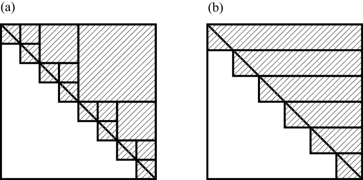
Figure 3: (a) Recursive and (b) row-wise splitting of the upper triangular part of a symmetric matrix.

Orthonormalize $(C_{\rm in})$:
(1) $S=C^{T}_{\rm in}C_{\rm in}$ DSYRK $O(m^{2}N)$ (2) Calculate $L$, where $S=LL^{T}$ DPOTRF $O(m^{3})$ (3) Calculate $L^{-1}$ DTRTRI $O(m^{3})$ (4) $C_{\rm out}=C_{\rm in}L^{-1}$ DTRMM $O(m^{2}N)$

Figure 4: Orthonormalization procedure based on the Cholesky factorization. Same notation as in Fig.2. $S$ is a symmetric matrix of dimension $m$, and $L$ is a lower triangular matrix of dimension $m$ (so is $L^{-1}$). On exit, $C_{\rm in}$ is overwritten by $C_{\rm out}$.

2.2 Mixed precision arithmetic

Here we present several ideas for improving the performance of the algorithm introduced in $\S$2.1 by taking advantage of inexpensive SP operations. The first approach is to perform all floating-point operations in DP (full DP), which will serve as a reference in the following. On the other hand, it is also possible to replace all DP operations by SP (full SP), which is expected to achieve the largest gain in terms of computational cost and memory usage. Unfortunately, as will be shown below, this approach does not provide sufficient accuracy, and thus is of limited use in real applications.

A more practical approach is to start from full DP, and incorporate SP operations progressively. Mixed precision variant-1 (MP1) is a conservative approach which aims at achieving a reasonable gain, while keeping full DP accuracy.
(i) The change of $C_{i}$, $\|C_{i+1}-C_{i}\|$, in Fig.1, will become much smaller than $\|C_{i}\|$ as convergence is approached. Therefore, $G_{i}$ and $P_{i}$ can be stored in memory in SP format without sacrificing accuracy. Here, the elements of $G_{i}$ are first calculated in DP to minimize round-off errors in Fig.2, followed by conversion to SP. Conversion between SP and DP is performed with the Fortran intrinsic functions Sngl and Dble. While this change alone leads to only a minor performance gain, a large gain can be made when used in conjunction with advanced preconditioners, as will be discussed in $\S$4. Furthermore, a significant reduction of memory usage is expected.
(ii) Similarly, the change of $C_{i}$ during the orthonormalization procedure shown in Fig.4 decreases from iteration to iteration. Therefore, after calculating $L^{-1}$, we introduce a DP matrix

$$L_{\rm D}=\mbox{diag}(L^{-1}),$$ (11)

and an SP matrix

$$L^{\prime}=L^{-1}-L_{\rm D},$$ (12)

where $L_{\rm D}\rightarrow I_{m}$ and $L^{\prime}\rightarrow 0$ as convergence is approached. Then, the last step can be rewritten as

$$C_{\rm out}=C_{\rm in}L_{\rm D}+C_{\rm in}L^{\prime},$$ (13)

where the first and the second terms are calculated in DP and SP, respectively. Obviously, the former cost is negligible, while the latter can be performed with an STRMM call instead of DTRMM. The final result, $C_{\rm out}$, is stored in DP format.

In addition to the changes noted above, further acceleration is achieved in the mixed precision variant-2 (MP2) by reducing the cost of evaluating the gradient in Fig.2, Algorithm-2, as follows. Since the computational cost of this procedure is dominated by steps-(1), (6), and (7), the two DGEMM calls in steps-(6) and (7) are replaced by SGEMM. The rest of the operations in this procedure, including step-(1), are performed in DP, which guarantees DP accuracy of the energy. Step-(5), corresponding to self-orthogonalization of the gradient, is also performed in DP, which allows us to reduce the round-off errors arising from the use of SGEMM in steps-(6) and (7) significantly. It is also preferable to set diag($H^{\prime}$)=0 explicitly after step-(6) to minimize the errors. Nevertheless, MP2 has the potential risk of obtaining inaccurate gradient when close to convergence.

When MP2 is used, all $O(m^{2}N)$ operations except the DSYRK call in the orthonormalization procedure are performed in SP. The performance and accuracy of these algorithms are compared in the next section.

3 Numerical results

Figure 5: Performance of matrix-matrix multiplications in SP (SGEMM) and DP (DGEMM).

All calculations shown here were performed on a single core of the 2.3 GHz AMD Opteron 6176 SE processor with CentOS 5.5 operating system, gfortran 4.1.2 compiler, and GotoBLAS2 numerical library [24].

We first show the performance of matrix-matrix multiplications in Fig.5. The SP routine (SGEMM) is found to be 1.85-1.95 times faster than the corresponding DP routine (DGEMM) when the matrix size is larger than 200.

Then, we compare the performance of full DP, MP1, MP2, and full SP for calculating the sum of the $m$ lowest eigenvalues of large sparse matrices corresponding to the two-dimensional discrete Laplacian under Dirichlet boundary conditions,

$${\cal H}_{N}=\left(\begin{array}[]{ccccc}D_{n}&-I_{n}&&&\smash{\lower 7.3194pt\hbox{\bg 0}}\\ -I_{n}&D_{n}&-I_{n}&&\\ &\ldots&\ldots&\ldots&\\ &&-I_{n}&D_{n}&-I_{n}\\ \smash{\hbox{\bg 0}}&&&-I_{n}&D_{n}\\ \end{array}\right)\in{\bf R}^{N\times N},$$ (14)

$$D_{n}=\left(\begin{array}[]{ccccc}4&-1&&&\smash{\lower 7.3194pt\hbox{\bg 0}}\\ -1&4&-1&&\\ &\ldots&\ldots&\ldots&\\ &&-1&4&-1\\ \smash{\hbox{\bg 0}}&&&-1&4\\ \end{array}\right)\in{\bf R}^{n\times n}.$$ (15)

The dimension $N$ is given by $N=n^{2}$, where $n$ denotes the grid size in each direction. The eigenvalues of ${\cal H}_{N}$ are given explicitly by

$$\lambda_{p,q}=4\left(\sin^{2}{\left(\frac{p\pi}{2(n+1)}\right)}+\sin^{2}{\left(\frac{q\pi}{2(n+1)}\right)}\right),\quad\quad p,q=1,2,...,n.$$ (16)

After sorting $\left\{\lambda_{p,q}\right\}$ in ascending order, we can calculate the exact value of $E_{\rm G}$ for any value of $m$. The above Hamiltonian represents free electrons confined in a square box, which is essentially a gapless system, as shown in Fig.6. Therefore, this problem is a stringent test for the trace minimization method which requires the presence of an energy gap.

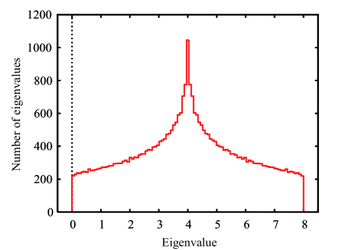
Figure 6: The eigenvalue distribution of ${\cal H}_{N}$ (Eq.(14)) for $N=192^{2}$.

Table 1: Performance of the four algorithms for iterative diagonalization of ${\cal H}_{N}$. $N_{\rm iter}$ denotes the number of iterations required to achieve $R<10^{-12}$ in the full DP run. All measurements are given in units of seconds per iteration. The numbers in parentheses indicate the percentage relative to full DP.

$N$	$m$	$E_{\rm G}$	$\epsilon_{\rm gap}$	$N_{\rm iter}$	Full DP	MP1	MP2	Full SP
962	220	35.25	6.2$\times$10-3	270	0.631	0.591(94%)	0.491(78%)	0.419(66%)
1922	220	8.991	1.9$\times$10-3	630	2.520	2.357(94%)	1.968(78%)	1.680(67%)
1922	534	50.90	2.5$\times$10-3	560	12.04	11.05(92%)	8.772(73%)	7.958(66%)
1922	1064	196.8	3.4$\times$10-3	460	45.38	41.01(90%)	30.52(67%)	28.04(62%)
1922	1519	395.6	2.7$\times$10-3	422	89.84	79.16(88%)	60.53(67%)	57.23(64%)

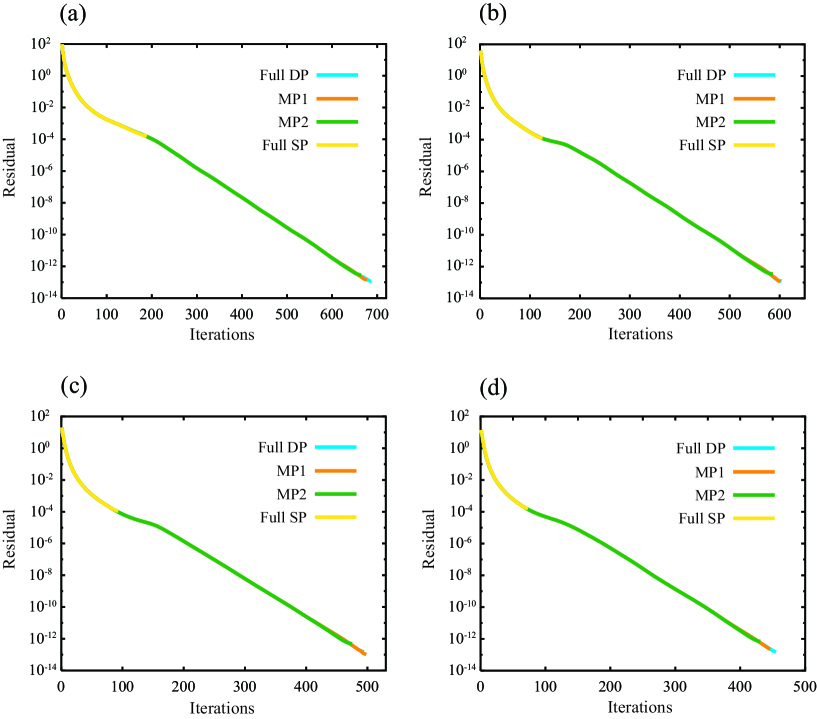
Figure 7: Convergence of the residual for $N=192^{2}$: (a) $m=220$, (b) $m=534$, (c) $m=1064$, and (d) $m=1519$.

In Table 1, we show the results of iterative diagonalization for several pairs of ($N,m$), following the algorithm presented in $\S$2.1. Here, the values of $m$ were chosen to satisfy $\epsilon_{\rm gap}>0$. For simplicity, the symmetry of $H^{\prime}$ was not exploited, and the initial guess $C_{0}$ was generated from random numbers, followed by orthonormalization. In Fig.7, we show the convergence of the residual at iteration $i$, defined by

$$R_{i}=\frac{E_{i}-E_{\rm G}}{E_{\rm G}}.$$ (17)

These results suggest that the performance of the four algorithms satisfies

$$\mbox{Full SP}\,>\,\mbox{MP2}\,>\,\mbox{MP1}\,>\,\mbox{Full DP},$$

where the differences tend to increase with $m$, but not with $N$. In particular, full SP is 30 - 40 % faster than full DP, which is consistent with the results for matrix multiplications. However, the accuracy of the results obtained from full SP is insufficient for most applications. Therefore, full SP should be used only for generating the initial guess [25].

In contrast, MP1 retains full DP accuracy for all values of $(N,m)$ shown in Table 1, while showing only a modest gain of $\approx$ 10 %.

MP2 is found to achieve a gain of over 30 % for large $m$, while keeping near DP accuracy. However, the accuracy of the converged solution deteriorates slowly with $m$, because the use of SP is not always appropriate for evaluating the gradient. We have found that if subspace rotation is performed occasionally to diagonalize $H$, this problem can be overcome, thus leading to full DP accuracy. Alternatively, one can simply switch from MP2 to MP1 (or full DP) algorithm when the residual is below a given tolerance. The latter approach is preferable in terms of the construction of conjugate directions [19], as well as the extrapolation of the initial guess [26].

4 Discussion

In $\S$2.1, we illustrated the implementation of the trace minimization method using the basic conjugate gradient method. In this section, we show how to improve the convergence rate of the conjugate gradient method by a linear transformation of the gradient

$$G^{\prime}=MG.$$ (18)

Here, $M\in{\bf R}^{N\times N}$ is a symmetric, positive definite matrix called a preconditioner, which should be a reasonable approximation to the inverse Hessian (See $\S$11 of Ref.[4]). Preconditioning allows us to reduce the number of iterations to reach convergence at the expense of increased cost per iteration. In electronic structure calculations, this generally leads to an increase in $O(mN)$ cost and a decrease in $O(m^{2}N)$ cost. Therefore, the choice of the preconditioner becomes more important for larger applications. In plane-wave-based electronic structure calculations, it is a common practice to use a diagonal matrix for $M$, which leads to a considerable reduction of the number of iterations [17] at a negligible cost.

However, more elaborate preconditioners have been developed beyond the diagonal approximation for plane waves [27], atomic orbitals [28], and real space basis sets [29, 30, 31]. These preconditioners significantly improve the convergence rate, while the computational cost of evaluating the right-hand side of Eq.(18) will become non-negligible. Since SP is generally sufficient for representing $G$, as already mentioned in $\S$2.2, the same will hold for $M$, unless $M$ is an ill-conditioned matrix. Therefore, the matrix multiplication of Eq.(18) can also be performed in SP, thus minimizing the overhead of preconditioning. The idea behind this approach is similar in spirit to the solution of linear equations discussed in Ref.[5]. These advanced preconditioners will be particularly beneficial when highly accurate methods [32] are used for the electronic structure calculations.

Although we have focused on the conjugate gradient method, the basic idea presented in this work should be equally valid for other iterative algorithms [33, 34, 35, 36, 37]. In our electronic structure code Femteck [12, 38], the trace minimization method is used in conjunction with the limited memory BFGS (Broyden-Fletcher-Goldfarb-Shanno) method [39, 40, 41, 42], which requires practically no line minimization. When the MP2 algorithm is used, together with a multigrid approximation to the inverse Hessian [31], the computational time for the ground-state calculation is reduced by a factor of about two in large-scale applications [10], compared with the full DP calculation using a diagonal approximation to the Hessian [41, 42]. If we start from a reasonable initial guess [26], the ground-state energy is obtained in 10-15 iterations in nonmetallic materials [9, 10].

5 Conclusion

We have shown in this work that iterative solution of the eigenvalue problem can be accelerated significantly by taking advantage of mixed precision arithmetic without relying on external devices. Even further improvement can be made by using problem-specific preconditioners which take into account nondiagonal elements. These methods will become more important with increasing problem size.

For most applications, MP2 is a good compromise between accuracy and computational cost. When highly accurate eigenvalues/vectors are desired, we recommend to switch from MP2 to MP1 (or full DP) at some point before the convergence slows down.

While the current implementation is designed for ground-state electronic structure calculations, it would also be interesting to investigate the use of mixed precision arithmetic in other problems such as the density-functional perturbation theory [43, 44, 45].

References

- [1] R. M. Martin, Electronic Structure: Basic Theory and Practical Methods, Cambridge University Press, 2004.
- [2] D. Marx, J. Hutter, Ab Initio Molecular Dynamics: Basic Theory and Advanced Methods, Cambridge University Press, 2009.
- [3] Y. Saad, J. R. Chelikowsky, S. M. Shontz, Numerical Methods for Electronic Structure Calculations of Materials, SIAM Rev. 52 (2010) 3-54.
- [4] Z. Bai, J. Demmel, J. Dongarra, A. Ruhe, H. van der Vorst, Templates for the Solution of Algebraic Eigenvalue Problems: A Practical Guide, SIAM, 2000.
- [5] M. Baboulin, A. Buttari, J. Dongarra, J. Kurzak, J. Langou, J. Langou, P. Luszczek, S. Tomov, Accelerating scientific computations with mixed precision algorithms, Comput. Phys. Commun. 180 (2009) 2526-2533.
- [6] M. Papadrakakis, N. Bitoulas, Accuracy and effectiveness of preconditioned conjugate gradient algorithms for large and ill-conditioned problems, Comput. Methods Appl. Mech. Engrg. 109 (1993) 219-232.
- [7] J. J. Dongarra, C. B. Moler, J. H. Wilkinson, Improving the accuracy of computed eigenvalues and eigenvectors, SIAM J. Numer. Anal. 20 (1983) 23-45.
- [8] V. Drygalla, Exploiting mixed precision for computing eigenvalues of symmetric matrices and singular values, PAMM 8 (2008) 10809-10810.
- [9] Y-K. Choe, E. Tsuchida, T. Ikeshoji, S. Yamanaka, S. Hyodo, Nature of proton dynamics in a polymer electrolyte membrane, nafion: a first-principles molecular dynamics study, Phys. Chem. Chem. Phys. 11 (2009) 3892-3899.
- [10] Y-K. Choe, E. Tsuchida, T. Ikeshoji, A. Ohira, K. Kidena, An ab initio modeling study on a modeled hydrated polymer electrolyte membrane, sulfonated polyethersulfone (SPES), J. Phys. Chem. B 114 (2010) 2411-2421.
- [11] A. H. Sameh, J. A. Wisniewski, A trace minimization algorithm for the generalized eigenvalue problem, SIAM J. Numer. Anal. 19 (1982) 1243-1259.
- [12] E. Tsuchida, M. Tsukada, Adaptive finite-element method for electronic-structure calculations, Phys. Rev. B 54 (1996) 7602-7605.
- [13] J. E. Pask, P. A. Sterne, Finite element methods in ab initio electronic structure calculations, Modelling Simul. Mater. Sci. Eng. 13 (2005) R71-R96.
- [14] J. M. Soler, E. Artacho, J. D. Gale, A. García, J. Junquera, P. Ordejón, D. Sánchez-Portal, The SIESTA method for ab initio order- materials simulation, J. Phys.: Condens. Matter 14 (2002) 2745-2779.
- [15] T. Ozaki, H. Kino, Numerical atomic basis orbitals from H to Kr, Phys. Rev. B 69 (2004) 195113.
- [16] I. Stich, R. Car, M. Parrinello, S. Baroni, Conjugate gradient minimization of the energy functional: A new method for electronic structure calculation, Phys. Rev. B 39 (1989) 4997-5004.
- [17] M. C. Payne, M. P. Teter, D. C. Allan, T. A. Arias, J. D. Joannopoulos, Iterative minimization techniques for ab initio total-energy calculations: molecular dynamics and conjugate gradients, Rev. Mod. Phys. 64 (1992) 1045-1097.
- [18] A. Edelman, S. T. Smith, On conjugate gradient-like methods for eigen-like problems, BIT 36 (1996) 494-508.
- [19] W. H. Press, S. A. Teukolsky, W. T. Vetterling, B. P. Flannery, Numerical Recipes in Fortran, Cambridge University Press, 1992.
- [20] R. D. King-Smith, D. Vanderbilt, First-principles investigation of ferroelectricity in perovskite compounds, Phys. Rev. B 49 (1994) 5828-5844.
- [21] J. F. Annett, Efficiency of algorithms for Kohn-Sham density functional theory, Comp. Mater. Sci. 4 (1995) 23-42.
- [22] N. Marzari, D. Vanderbilt, M. C. Payne, Ensemble density-functional theory for ab initio molecular dynamics of metals and finite-temperature insulators, Phys. Rev. Lett. 79 (1997) 1337-1340.
- [23] A. Sameh, Z. Tong, The trace minimization method for the symmetric generalized eigenvalue problem, J. Comput. Appl. Math. 123 (2000) 155-175.
- [24] K. Goto, R. van de Geijn, High-performance implementation of the level-3 BLAS, ACM Trans. Math. Softw. 35 (2008) 1-14.
- [25] R. Kosloff, H. Tal-Ezer, A direct relaxation method for calculating eigenfunctions and eigenvalues of the Schrödinger equation on a grid, Chem. Phys. Lett. 127 (1986) 223-230.
- [26] T. A. Arias, M. C. Payne, J. D. Joannopoulos, Ab initio molecular dynamics: Analytically continued energy functionals and insights into iterative solutions, Phys. Rev. Lett. 69 (1992) 1077-1080.
- [27] A. Sawamura, M. Kohyama, T. Keishi, An efficient preconditioning scheme for plane-wave-based electronic structure calculations, Comp. Mater. Sci. 14 (1999) 4-7.
- [28] V. Weber, J. VandeVondele, J. Hutter, A. M. N. Niklasson, Direct energy functional minimization under orthogonality constraints, J. Chem. Phys. 128 (2008) 084113.
- [29] J.-L. Fattebert, J. Bernholc, Towards grid-based O(N) density-functional theory methods: Optimized nonorthogonal orbitals and multigrid acceleration, Phys. Rev. B 62 (2000) 1713-1722.
- [30] T. Torsti et al., Three real-space discretization techniques in electronic structure calculations, Phys. Stat. Sol. (b) 243 (2006) 1016-1053.
- [31] E. Tsuchida, Ab initio molecular-dynamics study of liquid formamide, J. Chem. Phys. 121 (2004) 4740-4746.
- [32] M. Guidon, F. Schiffmann, J. Hutter, J. VandeVondele, Ab initio molecular dynamics using hybrid density functionals, J. Chem. Phys. 128 (2008) 214104.
- [33] E. R. Davidson, The iterative calculation of a few of the lowest eigenvalues and corresponding eigenvectors of large real-symmetric matrices, J. Comput. Phys. 17 (1975) 87-94.
- [34] J. Hutter, H. P. Lüthi, M. Parrinello, Electronic structure optimization in plane-wave-based density functional calculations by direct inversion in the iterative subspace, Comp. Mater. Sci. 2 (1994) 244-248.
- [35] G. L. G. Sleijpen, H. A. Van der Vorst, A Jacobi-Davidson iteration method for linear eigenvalue problems, SIAM Rev. 42 (2000) 267-293.
- [36] T. Ozaki, Efficient low-order scaling method for large-scale electronic structure calculations with localized basis functions, Phys. Rev. B 82 (2010) 075131.
- [37] D. R. Bowler, T. Miyazaki, Calculations for millions of atoms with density functional theory: linear scaling shows its potential, J. Phys.: Condens. Matter 22 (2010) 074207.
- [38] E. Tsuchida, M. Tsukada, Large-scale electronic-structure calculations based on the adaptive finite-element method, J. Phys. Soc. Jpn. 67 (1998) 3844-3858.
- [39] M. Head-Gordon, J. A. Pople, Optimization of wave function and geometry in the finite basis Hartree-Fock method, J. Phys. Chem. 92 (1988) 3063-3069.
- [40] D. C. Liu, J. Nocedal, On the limited memory BFGS method for large scale optimization, Math. Prog. 45 (1989) 503-528.
- [41] E. Tsuchida, An efficient algorithm for electronic-structure calculations, J. Phys. Soc. Jpn. 71 (2002) 197-203.
- [42] P. E. Gill, M. W. Leonard, Limited-memory reduced-Hessian methods for large-scale unconstrained optimization, SIAM J. Optim. 14 (2003) 380-401.
- [43] X. Gonze, C. Lee, Dynamical matrices, Born effective charges, dielectric permittivity tensors, and interatomic force constants from density-functional perturbation theory, Phys. Rev. B 55 (1997) 10355-10368.
- [44] A. Putrino, D. Sebastiani, M. Parrinello, Generalized variational density functional perturbation theory, J. Chem. Phys. 113 (2000) 7102-7109.
- [45] S. Baroni, S. de Gironcoli, A. Dal Corso, P. Giannozzi, Phonons and related crystal properties from density-functional perturbation theory, Rev. Mod. Phys. 73 (2001) 515-562.