Trading Order for Degree in Creative Telescoping

Abstract

We analyze the differential equations produced by the method of creative telescoping applied to a hyperexponential term in two variables. We show that equations of low order have high degree, and that higher order equations have lower degree. More precisely, we derive degree bounding formulas which allow to estimate the degree of the output equations from creative telescoping as a function of the order. As an application, we show how the knowledge of these formulas can be used to improve, at least in principle, the performance of creative telescoping implementations, and we deduce bounds on the asymptotic complexity of creative telescoping for hyperexponential terms.

1 Introduction

Creative telescoping is a technique for computing differential or difference equations satisfied by a given definite sum or integral. The technique became widely known through the work of Zeilberger (1991), who first observed that creative telescoping in combination with Gosper’s algorithm (Gosper, 1978) for indefinite hypergeometric summation leads to a complete algorithm for computing recurrence equations of definite hypergeometric sums. This algorithm is now known as Zeilberger’s algorithm (Zeilberger, 1990). In its original version, it accepts as input a bivariate proper hypergeometric term $f(n,k)$ and returns as output a linear recurrence equation with polynomial coefficients satisfied by the sum $F(n)=\sum_{k=a}^{b}f(n,k)$. An analogous algorithm for definite integration was given by Almkvist and Zeilberger (1990). This algorithm accepts as input a bivariate hyperexponential term $f(x,y)$ and returns as output a linear differential equation with polynomial coefficients satisfied by the integral $F(x)=\int_{\alpha}^{\beta}f(x,y)dy$. A summary of the method of creative telescoping for this case is given in Section 2 below. For further details, variations, and generalizations, consult for instance Petkovšek et al. (1997), Chyzak (2000), Schneider (2005), Chyzak et al. (2009), Kauers and Paule (2011). For implementations, see Paule and Schorn (1995), Chyzak (1998), Koepf (1998), Schneider (2004), Abramov et al. (2004), Koutschan (2009, 2010), etc.

The equations which can be found via creative telescoping have a certain order $r$ and polynomial coefficients of a certain degree $d$. But for a fixed integration problem, $r$ and $d$ are not uniquely determined. Instead, there are infinitely many points $(r,d)\in\mathbbm{N}^{2}$ such that creative telescoping can find an equation of order $r$ and degree $d$. These points form a region which is specific to the integration problem at hand. Figure 1 shows an example for such a region. Every point $(r,d)$ in the gray region corresponds to a differential equation of order $r$ and degree $d$ which creative telescoping can find for integrating the rational function

$$f(x,y) =\Bigl{(}3x^{2}y^{2}+9x^{2}y+9x^{2}+10xy^{2}+3xy+4x+1\Bigr{)}\Big{/}\Bigl{(}3x^{3}y^{3}+9x^{3}y^{2}+x^{3}y+3x^{3}$$

$$\qquad{}+7x^{2}y^{3}+8x^{2}y^{2}+5x^{2}+8xy^{3}+10xy^{2}+10xy+x+5y^{3}+10y^{2}+5y+5\Bigr{)}.$$

The picture indicates that low order equations have high degree, and that the degree decreases with increasing order. But what exactly is the shape of the gray region? And where does it come from? And how can it be exploited? These are the questions we address in this article.

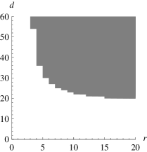
Figure 1: Sizes $(r,d)$ of creative telescoping relations for the integral of a certain rational function

How can it be exploited? There are two main reasons why the shape of the gray region is of interest. First, because it can be used to estimate the size of the output equations, and hence to derive bounds on the computational cost of computing them. Secondly, because it can be used to design more efficient algorithms by recognizing that some of the equations are cheaper than others.

An analysis of this kind was first undertaken by Bostan et al. (2007). They studied the problem of computing differential equations satisfied by a given algebraic function and found a similar phenomenon: low order equations have high degree and vice versa. Among other things, they found that an algebraic function with a minimal polynomial of degree $n$ satisfies a differential equation of order at most $n$ with polynomial coefficients of degree $\mathrm{O}(n^{3})$, but also a differential equation of order $6n$ whose coefficients have degree only $\mathrm{O}(n^{2})$. Their message is that trading order for degree can pay off.

The same phenomenon applies to creative telescoping, as was shown by Bostan et al. (2010) for the case of integrating rational functions. The results in the present article extend this work in two directions: First in that we consider the larger input class of hyperexponential terms, and second in that we give not only isolated degree estimates for some specific choices of $r$, but a curve which passes along the boundary of the gray region and thus establishes a degree estimate as a function of the order $r$.

Where does it come from? The standard argument for proving the existence of creative telescoping relations rests on the fact that linear systems of equations with more variables than equations must have a nontrivial solution. Every creative telescoping relation can be viewed as a solution of a certain linear system of equations which can be constructed from the data given in the input. There is some freedom in how to construct these systems, and it turns out that this freedom can be used for making the number of variables exceed the number of equations, and thus to enforce the existence of a nontrivial solution.

This reasoning not only implies the existence of equations and the termination of the algorithm which searches for them, but it also implies bounds on the output size and on the computational cost of the algorithm. But in order to obtain good bounds, the freedom in setting up the linear systems must be used carefully. For a good bound, we not only want that the number of variables exceeds the number of equations, but we also want this to happen already for a reasonably small system. The shape of the gray region originates from the smallest systems which have solutions.

Verbaeten (1974, 1976) introduced a technique which helps in keeping the size of the systems small. The idea is to saturate the linear systems by introducing additional variables in a way that avoids increasing the number of equations. We will make use of this idea in Section 3 where we propose a design for a parameterized family of linear systems whose solutions give rise to creative telescoping relations. Unfortunately, it requires some quite lengthy and technical calculations to translate this particular design into an inequality condition which rephrases the condition “number of variables $>$ number of equations” in precise terms. However, as a reward we obtain a good approximation to the gray region as the solution of this inequality.

What is the exact shape? We don’t know. All we can offer are some rational functions which describe the boundary of the region of all $(r,d)$ where the ansatz described in Section 3 has a solution (Theorem 14). The graphs of these rational functions are curves which pass approximately along the boundary of the gray region.

By construction, for all integer points $(r,d)$ above these graphs we can guarantee the existence of a creative telescoping relation of order $r$ with polynomial coefficients of degree $d$. But we have no proof that our curves are best possible. Experiments have shown that at least in some cases, our curve describes the boundary of the gray region exactly, or within a negligible error. In other cases, there remains a significant portion of the gray region below our curve when $r$ is large.

In cases where the curve from Theorem 14 is tight, we can compute the points $(r,d)$ for which certain interesting measures (such as computing time, output size, …) are minimized, as shown in Section 5. Even when the curve is not tight, these calculations still give rise to new asymptotic bounds (including the multiplicative constants) of the corresponding complexities. We expect that this data will be valuable for constructing the next generation of symbolic integration software.

2 Creative Telescoping for Hyperexponential Terms

We consider in this article only hyperexponential terms as integrands. Throughout the article, $\mathbbm{K}$ is a field of characteristic $0$, and $\mathbbm{K}(x,y)$ is the field of bivariate rational functions in $x$ and $y$ over $\mathbbm{K}$. Let $D_{x}$ and $D_{y}$ denote the derivations on $\mathbbm{K}(x,y)$ such that $D_{x}c=D_{y}c=0$ for all $c\in\mathbbm{K}$, and $D_{x}x=1$, $D_{x}y=0$, $D_{y}x=0$, $D_{y}y=1$. One can see that $D_{x}$ and $D_{y}$ commute with each other on $\mathbbm{K}(x,y)$. We say that a field $\mathbbm{E}$ containing $\mathbbm{K}(x,y)$ is a differential field extension of $\mathbbm{K}(x,y)$ if the derivations $D_{x}$ and $D_{y}$ are extended to derivations on $\mathbbm{E}$ and those extended derivations, still denoted by $D_{x}$ and $D_{y}$, commute with each other on $\mathbbm{E}$.

Definition 1.

An element $h$ of a differential field extension $\mathbbm{E}$ of $\mathbbm{K}(x,y)$ is called hyperexponential (over $\mathbbm{K}(x,y)$) if

$$\frac{D_{x}h}{h}\in\mathbbm{K}(x,y)\quad\text{and}\quad\frac{D_{y}h}{h}\in\mathbbm{K}(x,y).$$

When $h\in\mathbbm{E}$ is a hyperexponential term and $r_{1},r_{2}\in\mathbbm{K}(x,y)$ are such that $(D_{x}h)/h=r_{1}$ and $(D_{y}h)/h=r_{2}$, then $D_{x}D_{y}h=D_{y}D_{x}h$ implies $D_{y}r_{1}=D_{x}r_{2}$. Conversely, Christopher (1999) has shown for algebraically closed ground fields $\mathbbm{K}$ that for any two rational functions $r_{1},r_{2}\in\mathbbm{K}(x,y)$ with $D_{y}r_{1}=D_{x}r_{2}$ there exist $a/b\in\mathbbm{K}(x,y)$, $c_{0},\dots,c_{L}\in\mathbbm{K}[x,y]$ and $e_{1},\dots,e_{L}\in\mathbbm{K}$ with

$$r_{1}=\frac{D_{x}c_{0}}{c_{0}}+D_{x}\Bigl{(}\frac{a}{b}\Bigr{)}+\sum_{\ell=1}^{L}e_{\ell}\frac{D_{x}c_{\ell}}{c_{\ell}}\quad\text{and}\quad r_{2}=\frac{D_{y}c_{0}}{c_{0}}+D_{y}\Bigl{(}\frac{a}{b}\Bigr{)}+\sum_{\ell=1}^{L}e_{\ell}\frac{D_{y}c_{\ell}}{c_{\ell}}.$$

Together with Theorem 2 of Bronstein et al. (2005), it follows that there exists a differential field extension $\mathbbm{E}$ of $\mathbbm{K}(x,y)$ and an element $h\in\mathbbm{E}$ with $(D_{x}h)/h=r_{1}$ and $(D_{y}h)/h=r_{2}$ which we can write in the form

$$h=c_{0}\exp\Bigl{(}\frac{a}{b}\Bigr{)}\prod_{\ell=1}^{L}c_{\ell}^{e_{\ell}},$$

where $a\in\mathbbm{K}[x,y]$, $b,c_{0},\dots,c_{L}\in\mathbbm{K}[x,y]\setminus\{0\}$, $e_{1},\dots,e_{\ell}\in\mathbbm{K}$, and the expressions $\exp(a/b)$ and $c_{\ell}^{e_{\ell}}$ refer to elements of $\mathbbm{E}$ on which $D_{x}$ and $D_{y}$ act as suggested by the notation. We assume from now on that hyperexponential terms are always given in this form, and we use the letters $a,b,c_{0},\dots,c_{L},e_{1},\dots,e_{L}$ consistently throughout with the meaning they have here.

Example 2.

$h=\exp(x^{2}y)\sqrt{x-2y}$ is a hyperexponential term. We have

$$\frac{D_{x}h}{h} =\frac{1+4x^{2}y-8xy^{2}}{2x-4y}=2xy+\frac{1}{2x-4y}\in\mathbbm{K}(x,y),$$

$$\frac{D_{y}h}{h} =\frac{x^{3}-2x^{2}y-1}{x-2y}=x^{2}-\frac{1}{x-2y}\in\mathbbm{K}(x,y).$$

For this term, we can take $c_{0}=1$, $a=x^{2}y$, $b=1$, $c_{1}=x-2y$, $e_{1}=\tfrac{1}{2}$.

We may adopt the additional condition (without loss of generality) that the $c_{\ell}$ ($\ell>0$) are square free and pairwise coprime, and that $e_{\ell}\not\in\mathbbm{N}$ for all $\ell>0$. The estimates derived below do not depend on these additional conditions, but will typically not be sharp when they are not fulfilled. For simplicity, we will exclude throughout some trivial special cases by assuming that all $e_{\ell}$ are nonzero and that $\max\{\operatorname{deg}_{x}a,\operatorname{deg}_{x}b\}+\sum_{\ell=1}^{L}\operatorname{deg}_{x}c_{\ell}$ and $\max\{\operatorname{deg}_{y}a,\operatorname{deg}_{y}b\}+\sum_{\ell=1}^{L}\operatorname{deg}_{y}c_{\ell}$ are nonzero. These latter two conditions encode the requirement that $h$ is neither independent of $x$ nor independent of $y$, nor simply a polynomial.

Applied to the hyperexponential term $h$, the method of creative telescoping consists of finding, by whatever means, polynomials $p_{0},\dots,p_{r}\in\mathbbm{K}[x]$, not all zero, and a hyperexponential term $Q$ such that

$$p_{0}h+p_{1}D_{x}h+\cdots+p_{r}D_{x}^{r}h=D_{y}Q.$$

An equation of this form is called a creative telescoping relation for $h$, the differential operator $P:=p_{0}+p_{1}D_{x}+\cdots+p_{r}D_{x}^{r}$ appearing on the left is called the telescoper and $Q$ is called the certificate of the relation. The telescoper is required to be nonzero and free of $y$, but the certificate may be zero or it may involve both $x$ and $y$. When $p_{r}\neq 0$, the number $r$ is called the order of $P$, and $d:=\max_{i=0}^{r}\operatorname{deg}_{x}p_{i}$ is called its degree.

To motivate the form of a creative telescoping relation, assume that $h=h(x,y)$ can be interpreted as an actual function in $x$ and $y$ and consider the integral $f(x)=\int_{\alpha}^{\beta}h(x,y)dy$. Then integrating both sides of a creative telescoping relation implies that $f$ satisfies the inhomogeneous differential equation

$$p_{0}(x)f(x)+p_{1}(x)D_{x}f(x)+\cdots+p_{r}(x)D_{x}^{r}f(x)=\bigl{[}Q(x,y)\bigr{]}_{y=\alpha}^{\beta}.$$

In the frequent situation that the inhomogeneous part happens to evaluate to zero, this means that the telescoper of $h$ annihilates the integral $f$.

Example 3.

A creative telescoping relation for $h=\exp(x^{2}y)\sqrt{x-2y}$ is

$$(3x^{3}-6)h-2xD_{x}h=D_{y}\bigl{(}(3x-4y)h\bigr{)}.$$

It consists of the telescoper $P=(3x^{3}-6)-2xD_{x}$ and the certificate $Q=(3x-4y)h$. For the definite integral $f(x):=\int_{-\infty}^{x/2}\exp(x^{2}y)\sqrt{x-2y}dy$, we obtain the differential equation

$$(3x^{3}-6)f(x)-2xD_{x}f(x) =0.$$

Creative telescoping relations for hyperexponential terms can be found with the algorithm of Almkvist and Zeilberger (1990), which relies on a continuous analogue of Gosper’s summation algorithm. A more direct approach was considered by Apagodu (alias Mohammed) and Zeilberger (2005; 2006). After making a suitable choice for the denominator of $Q$, they fix an order $r$ and a degree $s$ for the numerator of $Q$, make an ansatz with undetermined coefficients, and obtain a linear system by comparing coefficients. Appropriate choices of $r$ and $s$ ensure that this linear system has a nontrivial solution, and also lead to a sharp bound on the order $r$ of the telescoper.

Let us illustrate this reasoning for the case where the integrand is a rational function $h=u/v\in\mathbbm{K}(x,y)$ with $\operatorname{deg}_{y}u<\operatorname{deg}_{y}v$ and $v$ irreducible. Fix some $r$. Then we have to find $p_{0},\dots,p_{r}\in\mathbbm{K}(x)$ and a rational function $Q\in\mathbbm{K}(x,y)$ with

$$p_{0}h+p_{1}D_{x}h+\cdots+p_{r}D_{x}^{r}h=D_{y}Q.$$

A reasonable choice for $Q$ is $Q=\bigl{(}\sum_{i=0}^{s}q_{i}y^{i}\bigr{)}/v^{r}$, where $s=\operatorname{deg}_{y}u+(r-1)\operatorname{deg}_{y}v$ and $q_{0},\dots,q_{s}$ are unknowns, because with this choice, both sides of the equation are equal to a rational function with the same denominator $v^{r+1}$ and numerators of degree at most $\operatorname{deg}_{y}u+r\operatorname{deg}_{y}v$ in $y$ in which the unknowns $p_{i}$ and $q_{j}$ appear linearly. Comparing coefficients with respect to $y$ on both sides leads to a homogeneous linear system of at most $1+\operatorname{deg}_{y}u+r\operatorname{deg}_{y}v$ equations with $(r+1)+(s+1)$ unknowns and coefficients in $\mathbbm{K}(x)$. This system will have a nontrivial solution if $r$ is chosen such that

$$(r+1)+(s+1)>\operatorname{deg}_{y}u+r\operatorname{deg}_{y}v+1\iff r\geq\operatorname{deg}_{y}v.$$

All these solutions must lead to a nonzero telescoper $P$ because any nontrivial solution with $P=0$ would have a nonzero certificate $Q$ with $D_{y}Q=0$, and this is impossible because $s$ was chosen such that the numerator of $Q$ has a strictly lower degree than its denominator.

We have thus shown the existence of telescopers of any order $r\geq\operatorname{deg}_{y}v$. This is a good bound, but it does not provide any estimate on their degrees $d$. We will next derive inequalities involving both $r$ and $d$ by constructing linear systems with coefficients in $\mathbbm{K}$ rather than in $\mathbbm{K}(x)$.

3 Shaping the Ansatz

Let $h$ be a hyperexponential term and consider an ansatz of the form

$$P=\sum_{i=0}^{r}\sum_{j=0}^{d_{i}}p_{i,j}x^{j}D_{x}^{i},\qquad Q=\biggl{(}\sum_{i=0}^{s_{1}}\sum_{j=0}^{s_{2}}q_{i,j}x^{i}y^{j}\biggr{)}\frac{h}{v}$$

for a telescoper $P$ and a certificate $Q$. The plan is to find a good choice for the parameters $r,s_{1},s_{2},v,d_{0},\dots,d_{r}$. The only restriction we have is that the linear system obtained from equating all the coefficients in the numerator of the rational function $(Ph-D_{y}Q)/h$ to zero should have a solution in which not all the $p_{i,j}$ are zero. The remaining freedom can be used to shape the ansatz such as to keep $d:=\max_{i=0}^{r}d_{i}$ small.

As a sufficient condition for the existence of a solution, we will require that the number of terms $x^{i}y^{j}$ in the numerator of the rational function $(Ph-D_{y}Q)/h$ (i.e., the number of equations) should be less than $\sum_{i=0}^{r}(d_{i}+1)+(s_{1}+1)(s_{2}+1)$ (i.e., the number of variables $p_{i,j}$ and $q_{i,j}$). As shown in the following example, this condition is really just sufficient, but not necessary.

Example 4.

Let $h=u/v$ be the rational function from the introduction. With $r=3$, $d_{0}=d_{1}=d_{2}=d_{3}=d=54$, and $Q=\bigl{(}\sum_{i=0}^{62}\sum_{j=0}^{8}q_{i,j}x^{i}y^{j}\bigr{)}\big{/}v^{3}$, comparing the coefficients of the numerator of $(Ph-D_{y}Q)/h$ to zero gives a linear system with $787$ variables and $792$ equations. This system has a nonzero solution although $792>787$.

This phenomenon is not only an unlikely coincidence in this particular example, but it happens systematically when the parameters of the ansatz are not well chosen. Estimates which are only based on balancing the number of variables and the number of equations will then overshoot. It is therefore preferable to shape the ansatz for $P$ and $Q$ in such a way that the linear system originating from it will have a nullspace whose dimension is exactly the difference between the number of equations and the number of variables (or 0 if there are more equations than variables).

The goal of this section is to describe our choice for the ansatz of telescoper and certificate. The form of the ansatz for the telescoper is given in Section 3.1, the certificate is discussed in Section 3.2. In the beginning, we collect some facts about the rational functions $(D_{x}^{i}h)/h$ which are used later for calculating how many equations a particular ansatz induces. The following notational conventions will be used throughout.

Notation 5.

• $\operatorname{lc}_{z}p$ and $\operatorname{deg}_{z}p$ refer to the leading coefficient and the degree of the polynomial $p$ with respect to the variable $z$, respectively. For the zero polynomial, we define $\operatorname{deg}_{z}0:=-\infty$ and $\operatorname{lc}_{z}0:=0$.

• $p^{\ast}$ refers to the square free part of the polynomial $p$ with respect to all its variables, e.g., $\bigl{(}(x+1)^{3}(y+3)^{2}\bigr{)}^{\ast}=(x+1)(y+3)$. Note that $p^{\ast}$ is only unique up to multiplication by elements from $\mathbbm{K}\setminus\{0\}$, but that for any choice of $p^{\ast}$, the degrees $\operatorname{deg}_{x}p^{\ast}$ and $\operatorname{deg}_{y}p^{\ast}$ are uniquely determined and we have that $p^{\ast}(D_{x}p)/p$ is a polynomial in $x$ and $y$. These are the only properties we will use.

• $z^{\underline{n}}:=z(z-1)(z-2)\cdots(z-n+1)$ and $z^{\overline{n}}:=z(z+1)(z+2)\cdots(z+n-1)$ denote the falling and rising factorials, respectively. For $n\leq 0$ we define $z^{\underline{n}}:=z^{\overline{n}}:=1$.

• If $z$ is a real number, then $z^{+}:=\max\{0,z\}$.

• If $z$ is a real number, then $\lfloor z\rfloor:=\max\{x\in\mathbbm{Z}:x\leq z\}$, $\lceil z\rceil:=\min\{x\in\mathbbm{Z}:x\geq z\}$, and $\lfloor z\rceil:=\lfloor z+\tfrac{1}{2}\rfloor$ denotes the nearest integer to $z$.

• If $\Phi$ is a formula then $[\![\Phi]\!]$ denotes the Iverson bracket, which evaluates to $1$ if $\Phi$ is true and to $0$ if $\Phi$ is false, e.g., $z^{+}=[\![z\geq 0]\!]z$; $\delta_{i,j}=[\![i=j]\!]$, etc.

Lemma 6.

Let $h$ be a hyperexponential term and $i\geq 0$.

1. If $\operatorname{deg}_{x}a>\operatorname{deg}_{x}b$, then

   $$\frac{D_{x}^{i}h}{h}=\frac{N_{i}}{c_{0}\bigl{(}bb^{\ast}\prod_{\ell=1}^{L}c_{\ell}\bigr{)}^{i}}$$

   for some polynomial $N_{i}\in\mathbbm{K}[x,y]$ with

   $$\operatorname{deg}_{x}N_{i} =\operatorname{deg}_{x}c_{0}+i\Bigl{(}\operatorname{deg}_{x}a+\operatorname{deg}_{x}b^{\ast}+\sum_{\ell=1}^{L}\operatorname{deg}_{x}c_{\ell}-1\Bigr{)},$$

   $$\operatorname{deg}_{y}N_{i} \leq\operatorname{deg}_{y}c_{0}+i\Bigl{(}\max\{\operatorname{deg}_{y}a,\operatorname{deg}_{y}b\}+\operatorname{deg}_{y}b^{\ast}+\sum_{\ell=1}^{L}\operatorname{deg}_{y}c_{\ell}\Bigr{)},$$

   $$\operatorname{lc}_{x}N_{i} =(\operatorname{lc}_{x}c_{0})\Bigl{(}\operatorname{lc}_{x}ab^{\ast}\prod_{\ell=1}^{L}c_{\ell}\Bigr{)}^{i}(\operatorname{deg}_{x}a-\operatorname{deg}_{x}b)^{i}.$$

2. If $\operatorname{deg}_{x}a\leq\operatorname{deg}_{x}b$, then

   $$\frac{D_{x}^{i}h}{h}=\frac{N_{i}}{c_{0}\bigl{(}bb^{\ast}\prod_{\ell=1}^{L}c_{\ell}\bigr{)}^{i}}$$

   for some polynomial $N_{i}\in\mathbbm{K}[x,y]$ with

   $$\operatorname{deg}_{x}N_{i} =\operatorname{deg}_{x}c_{0}+i\Bigl{(}\operatorname{deg}_{x}b+\operatorname{deg}_{x}b^{\ast}+\sum_{\ell=1}^{L}\operatorname{deg}_{x}c_{\ell}-1\Bigr{)}-[\![\omega\in\mathbbm{N}\land i>\omega]\!]\delta,$$

   $$\operatorname{deg}_{y}N_{i} \leq\operatorname{deg}_{y}c_{0}+i\Bigl{(}\max\{\operatorname{deg}_{y}a,\operatorname{deg}_{y}b\}+\operatorname{deg}_{y}b^{\ast}+\sum_{\ell=1}^{L}\operatorname{deg}_{y}c_{\ell}\Bigr{)},$$

   $$\operatorname{lc}_{x}N_{i} =\left\{\begin{array}[]{ll}(\operatorname{lc}_{x}c_{0})\bigl{(}\operatorname{lc}_{x}bb^{\ast}\prod\limits_{\ell=1}^{L}c_{\ell}\bigr{)}^{i}\omega^{\underline{i}}&\quad\text{if $\omega\not\in\mathbbm{N}$ or $i\leq\omega$;}\\ (\operatorname{lc}_{x}N_{\omega+1})\bigl{(}\operatorname{lc}_{x}bb^{\ast}\prod\limits_{\ell=1}^{L}c_{\ell}\bigr{)}^{i-(\omega+1)}(-\delta-1)^{\underline{i-(\omega+1)}}&\quad\text{if $\omega\in\mathbbm{N}$ and $i>\omega$,}\end{array}\right.$$

   where $\omega:=\operatorname{deg}_{x}c_{0}+\sum\limits_{\ell=1}^{L}e_{\ell}\operatorname{deg}_{x}c_{\ell}$ and, if $\omega\in\mathbbm{N}$,

   $$\delta:=\operatorname{deg}_{x}c_{0}+(\omega+1)\Bigl{(}\operatorname{deg}_{x}b+\operatorname{deg}_{x}b^{\ast}+\sum_{\ell=1}^{L}\operatorname{deg}_{x}c_{\ell}-1\Bigr{)}-\operatorname{deg}_{x}N_{\omega+1}\geq 1.$$

Proof..

All claims are proved by induction on $i$. For $i=0$, there is nothing to show in any of the cases. The calculations for the induction step $i\to i+1$ are as follows.

1. Let $v:=bb^{\ast}\prod_{\ell=1}^{L}c_{\ell}$ and write $m_{i}$ for the claimed value of $\operatorname{deg}_{x}N_{i}$. Then

   $$\frac{D_{x}^{i+1}h}{h} =D_{x}\biggl{(}\frac{N_{i}}{c_{0}v^{i}}c_{0}\exp\Bigl{(}\frac{a}{b}\Bigr{)}\prod_{\ell=1}^{L}c_{\ell}^{e_{\ell}}\biggr{)}\bigg{/}\biggl{(}c_{0}\exp\Bigl{(}\frac{a}{b}\Bigr{)}\prod_{\ell=1}^{L}c_{\ell}^{e_{\ell}}\biggr{)}$$

   $$=\frac{(D_{x}N_{i})v-iN_{i}D_{x}v}{c_{0}v^{i+1}}+\frac{N_{i}}{c_{0}v^{i}}\frac{(D_{x}a)b^{\ast}-ab^{\ast}(D_{x}b)/b}{bb^{\ast}}+\frac{N_{i}}{c_{0}v^{i}}\sum_{\ell=1}^{L}e_{\ell}\frac{D_{x}c_{\ell}}{c_{\ell}}$$

   $$=\frac{(D_{x}N_{i})v-iN_{i}D_{x}v+N_{i}\bigl{(}\prod\limits_{\ell=1}^{L}c_{\ell}\bigr{)}\bigl{(}(D_{x}a)b^{\ast}-ab^{\ast}\frac{D_{x}b}{b}\bigr{)}+N_{i}v\sum\limits_{\ell=1}^{L}e_{\ell}\frac{D_{x}c_{\ell}}{c_{\ell}}}{c_{0}v^{i+1}}.$$

   Since $\operatorname{deg}_{x}a>\operatorname{deg}_{x}b$ by assumption, we have

   $$\operatorname{deg}_{x}\biggl{(}(D_{x}N_{i})v-iN_{i}D_{x}v+N_{i}v\sum_{\ell=1}^{L}e_{\ell}\frac{D_{x}c_{\ell}}{c_{\ell}}\biggr{)}$$

   $$\qquad{}\leq\operatorname{deg}_{x}N_{i}+\operatorname{deg}_{x}v-1=m_{i}+\operatorname{deg}_{x}b^{\ast}+\operatorname{deg}_{x}b+\smash{\sum_{\ell=1}^{L}}\operatorname{deg}_{x}c_{\ell}-1$$

   $$\qquad{}<m_{i}+\operatorname{deg}_{x}a+\operatorname{deg}_{x}b^{\ast}+\sum_{\ell=1}^{L}\operatorname{deg}_{x}c_{\ell}-1=m_{i+1}.$$

   Furthermore, because of

   $$(D_{x}a)b^{\ast}-ab^{\ast}\frac{D_{x}b}{b}=(\operatorname{lc}_{x}a)(\operatorname{lc}_{x}b^{\ast})(\operatorname{deg}_{x}a-\operatorname{deg}_{x}b)x^{\operatorname{deg}_{x}a+\operatorname{deg}_{x}b^{\ast}-1}+\cdots$$

   we have

   $$N_{i}\Bigl{(}(D_{x}a)b^{\ast}-ab^{\ast}\frac{D_{x}b}{b}\Bigr{)}\prod_{\ell=1}^{L}c_{\ell} =(\operatorname{lc}_{x}N_{i})\Bigl{(}\operatorname{lc}_{x}ab^{\ast}\prod_{\ell=1}^{L}c_{\ell}\Bigr{)}(\operatorname{deg}_{x}a-\operatorname{deg}_{x}b)x^{m_{i+1}}+\cdots.$$

   This completes the proof that $(D_{x}^{i+1}h)/h$ has the denominator as claimed and that its numerator has degree and leading coefficient with respect to $x$ as claimed. The remaining degree bound with respect to $y$ follows from

   $$\operatorname{deg}_{y}\Bigl{(}(D_{x}N_{i})v-iN_{i}D_{x}v+N_{i}v\sum_{\ell=1}^{L}e_{\ell}\frac{D_{x}c_{\ell}}{c_{\ell}}\Bigr{)}$$

   $$\leq{} \underbrace{\operatorname{deg}_{y}c_{0}{+}i\Bigl{(}\operatorname{deg}_{y}b^{\ast}{+}\max\{\operatorname{deg}_{y}a,\operatorname{deg}_{y}b\}{+}\!\sum_{\ell=1}^{L}\operatorname{deg}_{y}c_{\ell}\Bigr{)}}_{\text{bounds $\operatorname{deg}_{y}N_{i}$}}+\underbrace{\operatorname{deg}_{y}b^{\ast}{+}\operatorname{deg}_{y}b{+}\!\sum_{\ell=1}^{L}\operatorname{deg}_{y}c_{\ell}}_{\text{bounds $\operatorname{deg}_{y}v$}}$$

   $$\leq{} \operatorname{deg}_{y}c_{0}+(i+1)\Bigl{(}\operatorname{deg}_{y}b^{\ast}+\max\{\operatorname{deg}_{y}a,\operatorname{deg}_{y}b\}+\sum_{\ell=1}^{L}\operatorname{deg}_{y}c_{\ell}\Bigr{)}$$

   and

   $$\operatorname{deg}_{y}\Bigl{(}N_{i}\Bigl{(}(D_{x}a)b^{\ast}-ab^{\ast}\frac{D_{x}b}{b}\Bigr{)}\prod\limits_{\ell=1}^{L}c_{\ell}\Bigr{)}$$

   $$\leq{} \underbrace{\operatorname{deg}_{y}c_{0}{+}i\Bigl{(}\operatorname{deg}_{y}b^{\ast}{+}\max\{\operatorname{deg}_{y}a,\operatorname{deg}_{y}b\}{+}\!\sum_{\ell=1}^{L}\operatorname{deg}_{y}c_{\ell}\Bigr{)}}_{\text{bounds $\operatorname{deg}_{y}N_{i}$}}+\underbrace{\operatorname{deg}_{y}b^{\ast}{+}\operatorname{deg}_{y}a{+}\sum_{\ell=1}^{L}\operatorname{deg}_{y}c_{\ell}}_{\text{bounds $\operatorname{deg}_{y}$ of the other factors}}$$

   $$\leq{} \operatorname{deg}_{y}c_{0}+(i+1)\Bigl{(}\operatorname{deg}_{y}b^{\ast}+\max\{\operatorname{deg}_{y}a,\operatorname{deg}_{y}b\}+\sum_{\ell=1}^{L}\operatorname{deg}_{y}c_{\ell}\Bigr{)}.$$

2. Again, let $v:=bb^{\ast}\prod_{\ell=1}^{L}c_{\ell}$ and write $m_{i}$ for the claimed value of $\operatorname{deg}_{x}N_{i}$. Then, like in part 1,

   $$\frac{D_{x}^{i+1}h}{h}=\frac{(D_{x}N_{i})v-iN_{i}D_{x}v+N_{i}\bigl{(}\prod\limits_{\ell=1}^{L}c_{\ell}\bigr{)}\bigl{(}(D_{x}a)b^{\ast}-ab^{\ast}\frac{D_{x}b}{b}\bigr{)}+N_{i}v\sum\limits_{\ell=1}^{L}e_{\ell}\frac{D_{x}c_{\ell}}{c_{\ell}}}{c_{0}v^{i+1}}.$$

   First consider the case $\omega\not\in\mathbbm{N}$ or $i\leq\omega$.

   Since $\operatorname{deg}_{x}a\leq\operatorname{deg}_{x}b$ by assumption, and because of

   $$(D_{x}a)b^{\ast}-ab^{\ast}\frac{D_{x}b}{b}=(\operatorname{lc}_{x}a)(\operatorname{lc}_{x}b^{\ast})(\operatorname{deg}_{x}a-\operatorname{deg}_{x}b)x^{\operatorname{deg}_{x}a+\operatorname{deg}_{x}b^{\ast}-1}+\cdots,$$

   we now have

   $$\operatorname{deg}_{x}\Bigl{(}N_{i}\Bigl{(}(D_{x}a)b^{\ast}-ab^{\ast}\frac{D_{x}b}{b}\Bigr{)}\prod_{\ell=1}^{L}c_{\ell}\Bigr{)}$$

   $$\quad{}<m_{i}+\operatorname{deg}_{x}b+\operatorname{deg}_{x}b^{\ast}-1+\sum_{\ell=1}^{L}\operatorname{deg}_{x}c_{\ell}=m_{i+1}.$$

   Note that this estimate is also strict when $\operatorname{deg}_{x}a=\operatorname{deg}_{x}b$ because the coefficient of $x^{\operatorname{deg}_{x}a+\operatorname{deg}_{x}b^{\ast}-1}$ in $(D_{x}a)b^{\ast}-ab^{\ast}(D_{x}b)/b$ contains the factor $\operatorname{deg}_{x}a-\operatorname{deg}_{x}b$, which vanishes in this case.

   Next, using the induction hypothesis, we have

   $$(D_{x}N_{i})v-iN_{i}D_{x}v+N_{i}v\sum_{\ell=1}^{L}e_{\ell}\frac{D_{x}c_{\ell}}{c_{\ell}}$$

   $$={} (\operatorname{lc}_{x}N_{i})(\operatorname{lc}_{x}v)\Bigl{(}\operatorname{deg}_{x}N_{i}-i\operatorname{deg}_{x}v+\sum_{\ell=1}^{L}e_{\ell}\operatorname{deg}_{x}c_{\ell}\Bigr{)}x^{\operatorname{deg}_{x}N_{i}+\operatorname{deg}_{x}v-1}+\cdots$$

   $$={} (\operatorname{lc}_{x}c_{0})\Bigl{(}\operatorname{lc}_{x}bb^{\ast}\prod_{\ell=1}^{L}c_{\ell}\Bigr{)}^{i}\omega^{\underline{i}}\,(\operatorname{lc}_{x}v)\Bigl{(}m_{i}-i\operatorname{deg}_{x}v+\sum_{\ell=1}^{L}e_{\ell}\operatorname{deg}_{x}c_{\ell}\Bigr{)}x^{m_{i}+\operatorname{deg}_{x}v-1}+\cdots$$

   $$={} (\operatorname{lc}_{x}c_{0})\Bigl{(}\operatorname{lc}_{x}bb^{\ast}\prod_{\ell=1}^{L}c_{\ell}\Bigr{)}^{i+1}\omega^{\underline{i}}\Bigl{(}\operatorname{deg}_{x}c_{0}+\sum_{\ell=1}^{L}e_{\ell}\operatorname{deg}_{x}c_{\ell}-i\Bigr{)}x^{m_{i+1}}+\cdots$$

   $$={} (\operatorname{lc}_{x}c_{0})\Bigl{(}\operatorname{lc}_{x}bb^{\ast}\prod_{\ell=1}^{L}c_{\ell}\Bigr{)}^{i+1}\omega^{\underline{i+1}}x^{m_{i+1}}+\cdots.$$

   Since $\omega^{\underline{i+1}}\neq 0$ when $\omega\not\in\mathbbm{N}$ or $i+1\leq\omega$, this completes the proof that $(D_{x}^{i+1}h)/h$ has the denominator as claimed and that its numerator has degree and leading coefficient with respect to $x$ as claimed. The degree bounds with respect to $y$ are shown exactly as in part 1.

   Now consider the case where $\omega\in\mathbbm{N}$ and $i>\omega$. In this case, we start the induction at $i=\omega+1$. The induction base follows from the calculations carried out above for $i\geq\omega$, the fact $\omega^{\underline{\omega+1}}=0$, and the definition of $\delta$. (Note that $\omega^{\underline{\omega+1}}=0$ also implies $\delta\geq 1$.) For the induction step $i\mapsto i+1$, we have, similar as before,

   $$\operatorname{deg}_{x}\Bigl{(}N_{i}\Bigl{(}(D_{x}a)b^{\ast}-ab^{\ast}\frac{D_{x}b}{b}\Bigr{)}\prod_{\ell=1}^{L}c_{\ell}\Bigr{)}<m_{i+1}$$

   and

   $$(D_{x}N_{i})v-iN_{i}D_{x}v+N_{i}v\sum_{\ell=1}^{L}e_{\ell}\frac{D_{x}c_{\ell}}{c_{\ell}}$$

   $$={} (\operatorname{lc}_{x}N_{i})(\operatorname{lc}_{x}v)\Bigl{(}m_{i}-i\operatorname{deg}_{x}v+\sum_{\ell=1}^{L}e_{\ell}\operatorname{deg}_{x}c_{\ell}\Bigr{)}x^{m_{i}+\operatorname{deg}_{x}v-1}+\cdots$$

   $$={} (\operatorname{lc}_{x}N_{i})(\operatorname{lc}_{x}v)\Bigl{(}\operatorname{deg}_{x}c_{0}+i(\operatorname{deg}_{x}v-1)-\delta-i\operatorname{deg}_{x}v+\sum_{\ell=1}^{L}e_{\ell}\operatorname{deg}_{x}c_{\ell}\Bigr{)}x^{m_{i+1}}+\cdots$$

   $$={} (\operatorname{lc}_{x}N_{\omega+1})\Bigl{(}\operatorname{lc}_{x}bb^{\ast}\prod_{\ell=1}^{L}c_{\ell}\Bigr{)}^{i-(\omega+1)}(-\delta-1)^{\underline{i-(\omega+1)}}(\operatorname{lc}_{x}v)(\omega-\delta-i)x^{m_{i+1}}+\cdots$$

   $$={} (\operatorname{lc}_{x}N_{\omega+1})\Bigl{(}\operatorname{lc}_{x}bb^{\ast}\prod_{\ell=1}^{L}c_{\ell}\Bigr{)}^{i+1-(\omega+1)}(-\delta-1)^{\underline{i+1-(\omega+1)}}x^{m_{i+1}}+\cdots$$

   Because of $\delta>0$, the factor $(-\delta-1)^{\underline{i-(\omega+1)}}$ is nonzero for all $i>\omega$.    $\Box$

Example 7.

The case when $h=u/v$ is a rational function is covered by part 2 of the lemma. For example, for $h=(2x^{5}-3x^{4}+5)/(3x^{3}-4x+8)$ we can take $c_{0}=2x^{5}-3x^{4}+5$, $a=0$, $b=1$, $L=1$, $c_{1}=3x^{3}-4x+8$, $e_{1}=-1$. Direct calculation of the derivatives gives

$i$	0	1	2	3	4	5	6
$\operatorname{deg}_{x}c_{0}c_{1}^{i}(D_{x}^{i}h)/h$	5	7	9	8	10	12	14
$\operatorname{lc}_{x}c_{0}c_{1}^{i}(D_{x}^{i}h)/h$	2	12	36	1512	$-18144$	272160	$-4898880$

The lemma makes no statement about the degree or leading coefficient in the case $i=\omega+1=3$, but knowing these, it correctly predicts all the other data in the table. In this example, we have $\delta=3=\omega+1$. This is not a coincidence, as we shall show next.

Lemma 8.

Let $h$ be a hyperexponential term with $\operatorname{deg}_{x}a\leq\operatorname{deg}_{x}b$, and let $\omega$ and $\delta$ be as in Lemma 6.(2), $\omega\in\mathbbm{N}$. Then $\delta\geq\omega+1$.

Proof..

Rewrite $h=c_{0}\exp(\frac{a}{b})\prod_{\ell=1}^{L}c_{\ell}^{e_{\ell}}=\bar{c}_{0}\exp(\frac{a}{b})\prod_{\ell=1}^{L+2}\bar{c}_{\ell}^{\bar{e}_{\ell}}$ with $\bar{c}_{0}=x^{\omega}$, $\bar{c}_{\ell}=c_{\ell}$ ($\ell=1,\dots,L$), $\bar{e}_{\ell}=e_{\ell}$ ($\ell=1,\dots,L$), $\bar{c}_{L+1}=c_{0}$, $\bar{e}_{L+1}=1$, $\bar{c}_{L+2}=x$, $\bar{e}_{L+2}=-\omega$. The rational functions $(D_{x}^{i}h)/h$ are of course independent of the representation of $h$, but the representations of these rational functions which are given in Lemma 6 are not. The representation obtained for the new representation of $h$ is obtained from the original representation by multiplying numerator and denominator by $x^{\omega+i}c_{0}^{i-1}$. Observe that this modification does not influence the values for $\omega$ or $\delta$. It is therefore sufficient to prove the claim for terms of the form $h=x^{\omega}\bar{h}$, where $\bar{h}$ is some hyperexponential term for which the value of $\omega$ is zero. We do so by induction on $\omega$. For $\omega=0$, we have $\delta\geq 1=\omega+1$ already by Lemma 6.(2). Now assume that $\omega\geq 0$ is such that for $x^{\omega}\bar{h}$ the degree drop $\bar{\delta}$ is $\omega+1$ or more. Then for $h=x^{\omega+1}\bar{h}=x(x^{\omega}\bar{h})$ we have $D_{x}h=x^{\omega}\bar{h}+xD_{x}(x^{\omega}\bar{h})$, $D_{x}^{2}h=2D_{x}(x^{\omega}\bar{h})+xD_{x}^{2}(x^{\omega}\bar{h})$, and so on, all the way down to

$$D_{x}^{\omega+2}h =(\omega+2)D_{x}^{\omega+1}(x^{\omega}\bar{h})+xD_{x}^{\omega+2}(x^{\omega}\bar{h})$$

$$=(\omega+2)\frac{N_{\omega+1}}{x^{\omega}v^{\omega+1}}x^{\omega}\bar{h}+x\frac{N_{\omega+2}}{x^{\omega}v^{\omega+2}}x^{\omega}\bar{h}$$

$$=\frac{(\omega+2)N_{\omega+1}v+xN_{\omega+2}}{v^{\omega+2}}\bar{h},$$ (1)

where $N_{\omega+1}$ and $N_{\omega+2}$ are as in Lemma 6 and $v$ refers to the denominator stated there. If $\delta$ denotes the degree drop for $h$, then this calculation implies $\delta\geq\bar{\delta}$. By induction hypothesis, we have $\bar{\delta}\geq\omega+1$. If in fact $\bar{\delta}\geq\omega+2$, then we are done. Otherwise, if $\bar{\delta}=\omega+1$, then

$$\operatorname{lc}_{x}N_{\omega+2}=(-\bar{\delta}-1)\operatorname{lc}_{x}N_{\omega+1}\operatorname{lc}_{x}v=-(\omega+2)\operatorname{lc}_{x}N_{\omega+1}\operatorname{lc}_{x}v$$

by Lemma 6, so the leading terms of the two polynomials in the numerator of (1) cancel, and therefore $\delta>\omega+1$ also in this case.    $\Box$

Experiments suggest that the bound in Lemma 8 is tight in the sense that we have $\delta=\omega+1$ for almost all hyperexponential terms $h$. But there do exist situations with $\delta>\omega+1$. For example, it can be shown that for $h=c_{0}\exp(a/b)$ with $\operatorname{deg}_{x}b-\operatorname{deg}_{x}a>\operatorname{deg}_{x}c_{0}=\omega$ we have $\delta\geq\operatorname{deg}_{x}b-\operatorname{deg}_{x}a$.

Also Lemma 6 is not necessarily sharp for degenerate choices of $h$. In particular, we do not claim that the numerators and denominators stated in Lemma 6 are coprime. It may be possible to carry out a finer analysis by considering the square free decomposition of $c_{0}$, or by taking into account possible common factors between $b$ and the $c_{\ell}$, or by handling the $c_{\ell}$ which do not involve $x$ separately. For our purpose, we believe that the statements given above form a reasonable compromise between sharpness of the statements and readability of the derivation.

Several aspects of the formulas in Lemma 6 are important. One of them is that the denominators corresponding to lower derivatives divide those corresponding to higher derivatives. This has the consequence that when the linear combination $Ph$ is brought on a common denominator, the degree of the numerator will not grow drastically. In a sense, this fact is the main reason why creative telescoping works at all. Our next step is to bring the formulas from Lemma 6 on a common denominator.

Lemma 9.

Let $h$ be a hyperexponential term and $r,i\in\mathbbm{Z}$ with $r\geq i\geq 0$.

1. If $\operatorname{deg}_{x}a>\operatorname{deg}_{x}b$, then

   $$\frac{D_{x}^{i}h}{h}=\frac{N_{r,i}}{c_{0}\bigl{(}bb^{\ast}\prod_{\ell=1}^{L}c_{\ell}\bigr{)}^{r}}$$

   for some $N_{r,i}\in\mathbbm{K}[x,y]$ with

   $$\operatorname{deg}_{x}N_{r,i} =\operatorname{deg}_{x}c_{0}+r\Bigl{(}\operatorname{deg}_{x}b^{\ast}+\operatorname{deg}_{x}b+\sum_{\ell=1}^{L}\operatorname{deg}_{x}c_{\ell}\Bigr{)}+i\Bigl{(}\operatorname{deg}_{x}a-\operatorname{deg}_{x}b-1\Bigr{)}$$

   $$\operatorname{deg}_{y}N_{r,i} \leq\operatorname{deg}_{y}c_{0}+r\Bigl{(}\operatorname{deg}_{y}b^{\ast}+\max\{\operatorname{deg}_{y}a,\operatorname{deg}_{y}b\}+\sum_{\ell=1}^{L}\operatorname{deg}_{y}c_{\ell}\Bigr{)},$$

   $$\operatorname{lc}_{x}N_{r,i} =(\operatorname{lc}_{x}c_{0})(\operatorname{lc}_{x}a)^{i}(\operatorname{lc}_{x}b)^{r-i}(\operatorname{lc}_{x}b^{\ast})^{r}\Bigl{(}\operatorname{lc}_{x}\prod\limits_{\ell=1}^{L}c_{\ell}\Bigr{)}^{r}\bigl{(}\operatorname{deg}_{x}a-\operatorname{deg}_{x}b\bigr{)}^{i}.$$

2. If $\operatorname{deg}_{x}a\leq\operatorname{deg}_{x}b$, then

   $$\frac{D_{x}^{i}h}{h}=\frac{N_{r,i}}{c_{0}\bigl{(}bb^{\ast}\prod_{\ell=1}^{L}c_{\ell}\bigr{)}^{r}}$$

   for some $N_{r,i}\in\mathbbm{K}[x,y]$ with

   $$\operatorname{deg}_{x}N_{r,i} =\operatorname{deg}_{x}c_{0}+r\Bigl{(}\operatorname{deg}_{x}b^{\ast}+\operatorname{deg}_{x}b+\sum_{\ell=1}^{L}\operatorname{deg}_{x}c_{\ell}\Bigr{)}-i-[\![\omega\in\mathbbm{N}\land i>\omega]\!]\delta,$$

   $$\operatorname{deg}_{y}N_{r,i} \leq\operatorname{deg}_{y}c_{0}+r\Bigl{(}\operatorname{deg}_{y}b^{\ast}+\max\{\operatorname{deg}_{y}a,\operatorname{deg}_{y}b\}+\sum_{\ell=1}^{L}\operatorname{deg}_{y}c_{\ell}\Bigr{)},$$

   $$\operatorname{lc}_{x}N_{r,i} =\left\{\begin{array}[]{ll}(\operatorname{lc}_{x}c_{0})(\operatorname{lc}_{x}bb^{\ast})^{r}\bigl{(}\operatorname{lc}_{x}\prod\limits_{\ell=1}^{L}c_{\ell}\bigr{)}^{r}\omega^{\underline{i}}&\quad\text{if $\omega\not\in\mathbbm{N}$ or $i\leq\omega$;}\\ (\operatorname{lc}_{x}N_{\omega+1})\bigl{(}\operatorname{lc}_{x}bb^{\ast}\prod\limits_{\ell=1}^{L}c_{\ell}\bigr{)}^{r-(\omega+1)}(-\delta-1)^{\underline{i-(\omega+1)}}&\quad\text{if $\omega\in\mathbbm{N}$ and $i>\omega$,}\end{array}\right.$$

   where $\omega$, $\delta$, and $\operatorname{lc}_{x}N_{\omega+1}$ are as in Lemma 6.(2).

Proof..

Both parts follow directly from the respective parts of Lemma 6 by multiplying numerator and denominator of the representations stated there by $\bigl{(}bb^{\ast}\prod_{\ell=1}^{L}c_{\ell}\bigr{)}^{r-i}$.    $\Box$

Since we will be frequently referring to the quantities in this lemma, it seems convenient to adopt the following definition.

Definition 10.

For a hyperexponential term $h$, let

$$\alpha =\operatorname{deg}_{x}b^{\ast}+\operatorname{deg}_{x}b+\sum_{\ell=1}^{L}\operatorname{deg}_{x}c_{\ell}, \qquad\beta =\operatorname{deg}_{x}a-\operatorname{deg}_{x}b-1,$$

$$\gamma =\operatorname{deg}_{y}b^{\ast}+\max\{\operatorname{deg}_{y}a,\operatorname{deg}_{y}b\}+\sum_{\ell=1}^{L}\operatorname{deg}_{y}c_{\ell}, \omega =\operatorname{deg}_{x}c_{0}+\sum_{\ell=1}^{L}e_{\ell}\operatorname{deg}_{x}c_{\ell}.$$

If $\operatorname{deg}_{x}a\leq\operatorname{deg}_{x}b$ and $\omega\in\mathbbm{N}$, we further let $\delta$ be any integer with

$$\omega+1\leq\delta\leq\operatorname{deg}_{x}c_{0}+(\omega+1)(\alpha-1)-\operatorname{deg}_{x}\biggl{(}c_{0}\Bigl{(}bb^{\ast}\prod_{\ell=1}^{L}c_{\ell}\Bigr{)}^{\omega+1}\frac{D_{x}^{\omega+1}h}{h}\biggr{)}.$$

Otherwise, if $\operatorname{deg}_{x}a>\operatorname{deg}_{x}b$ or $\omega\not\in\mathbbm{N}$, let $\delta=0$. Finally, we define the following flags:

$$\phi_{1}=[\![\tfrac{\operatorname{lc}_{x}a}{\operatorname{lc}_{x}b}\in\mathbbm{K}]\!],\qquad\phi_{2}=[\![\tfrac{\operatorname{lc}_{x}a}{\operatorname{lc}_{x}b}\in\mathbbm{K}\land\beta=0]\!],$$

$$\phi_{3}=[\![\,\tfrac{a}{b}\in\mathbbm{K}(x)\land\forall\ \ell:(\operatorname{deg}_{y}c_{\ell}=0\lor e_{\ell}\in\mathbbm{Z})\land\operatorname{deg}_{y}c_{0}\geq{\textstyle\sum\limits_{\ell=1}^{L}}e_{\ell}\operatorname{deg}_{y}c_{\ell}]\!]\,.$$

Note that none of these parameters depends on $r$ or $i$. The flags $\phi_{k}$ ($k=1,2,3$) are in $\{0,1\}$, $\omega$ belongs to $\mathbbm{K}$, $\beta$ belongs to $\mathbbm{N}\cup\{-1\}$, and all other parameters are positive integers. The best value for $\delta$ is the right bound of the specified range, but since this value cannot be directly read of from the input, we do not insist that $\delta$ be equal to this value, but we allow $\delta$ to be any number between the bound from Lemma 8 and the true degree drop. The flags $\phi_{1}$ and $\phi_{2}$ will be used below in the ansatz for the telescoper, $\phi_{3}$ will play a role afterwards in the ansatz for the certificate.

In terms of the parameters defined in Definition 10, the degree bounds of Lemma 9 simplify to

$$\operatorname{deg}_{x}N_{r,i}\leq\operatorname{deg}_{x}c_{0}+\alpha r+\max\{\beta,-1\}i-[\![\omega\in\mathbbm{N}\land i>\omega]\!]\delta,$$

$$\operatorname{deg}_{y}N_{r,i}\leq\operatorname{deg}_{y}c_{0}+\gamma r.$$

3.1 The Ansatz for the Telescoper

Lemma 9 suggests reasonable choices for the degrees $d_{i}$ in the ansatz for $P$. In particular, our choice is based on the following features of the formulas in Lemma 9.

• The degree of the numerator in $(D_{x}^{i}h)/h$ varies with $i$. A good choice for the degrees $d_{i}$ will compensate for this variation, taking higher values for $d_{i}$ when the numerator of $(D_{x}^{i}h)/h$ has low degree, and vice versa. This is the key idea of the Verbaeten completion (Verbaeten, 1974, 1976; Wegschaider, 1997).

• The leading coefficients of $N_{r,i}$ ($i>0$) are polynomials in $y$, but in case 2, most of them are $\mathbbm{K}$-multiples of each other. When $a$ and $b$ are such that $(\operatorname{lc}_{x}a)/(\operatorname{lc}_{x}b)\in\mathbbm{K}$, then this is also true in case 1. We will use this fact for eliminating several equations at the cost of a single variable.

Before describing the ansatz for $P$ in full generality, we motivate the construction by an example.

Example 11.

Suppose that $h$ is hyperexponential with $\operatorname{lc}_{x}a=\operatorname{lc}_{x}b$, $\beta=1$ (case 1 of Lemma 9), and $\operatorname{deg}_{x}c_{0}=0$.

Let $r=5$ and $d=7$. We want to choose $d_{i}$ such that $\max_{i=0}^{5}d_{i}=7$ and the ansatz

$$P=\sum_{i=0}^{5}\sum_{j=0}^{d_{i}}p_{i,j}x^{j}D_{x}^{i}$$

leads to “many” variables but only “few” equations. The choice with most variables is clearly to set $d_{i}=d=7$ for all $i$. But this ansatz leads to quite many equations. Each term $x^{j}D_{x}^{i}$ contributes to the common numerator a polynomial $x^{j}N_{5,i}$ whose degree in $x$ is $5\alpha+i+j$ and whose degree in $y$ is at most $5\gamma$. Because of the term $x^{7}D_{x}^{5}$, we must expect up to $(5\alpha+13)(5\gamma+1)$ terms in the numerator. This is the expected number of equations in the linear system resulting from coefficient comparison.

If we remove the term $x^{7}D_{x}^{5}$ from the ansatz, i.e., if we choose $d_{0}=\cdots=d_{4}=7$, $d_{5}=6$, then the number of equations drops to $(5\alpha+12)(5\gamma+1)$ because all terms $x^{j}D_{x}^{i}$ other than $x^{7}D_{x}^{5}$ contribute only polynomials $x^{j}N_{5,i}$ of lower degree. We save $5\gamma+1$ equations at the cost of removing a single variable. Removing also the terms $x^{7}D_{x}^{4}$ and $x^{6}D_{x}^{5}$ lowers the number of equations further to $(5\alpha+11)(5\gamma+1)$, and in general, for any $0\leq w\leq 5$, choosing $d_{i}=7-(w+i-5)^{+}$ ($i=0,\dots,5$) leads to $(5\alpha+13-w)(5\gamma+1)$ equations. The number of variables is $(5+1)(7+1)-\sum_{k=1}^{w}k=48-\tfrac{1}{2}w(w+1)$.

If $w>1$, we can introduce $w-1$ new variables by exploiting the second feature of the formulas in Lemma 9 as follows. Consider the choice $w=3$, i.e., the terms $x^{j}D_{x}^{i}$ with $i+j\geq 10$ have been removed from the ansatz. We reintroduce the terms $x^{7}D_{x}^{3}$, $x^{6}D_{x}^{4}$, $x^{5}D_{x}^{5}$ by adding

$$p_{3,7}\bigl{(}(\operatorname{deg}_{x}a-\operatorname{deg}_{x}b)^{2}x^{7}D_{x}^{3}-x^{5}D_{x}^{5}\bigr{)}+p_{4,6}\bigl{(}(\operatorname{deg}_{x}a-\operatorname{deg}_{x}b)x^{6}D_{x}^{4}-x^{5}D_{x}^{5}\bigr{)}$$

to the ansatz, getting back the two variables $p_{3,7}$ and $p_{4,6}$ but no new equations, because, according to Lemma 9.(1), the assumption $\operatorname{lc}_{x}a=\operatorname{lc}_{x}b$ implies

$$(\operatorname{deg}_{x}a-\operatorname{deg}_{x}b)^{2}\operatorname{lc}_{x}N_{5,3}=\operatorname{lc}_{x}N_{5,5}\quad\text{and}\quad(\operatorname{deg}_{x}a-\operatorname{deg}_{x}b)\operatorname{lc}_{x}N_{5,4}=\operatorname{lc}_{x}N_{5,5}.$$

The final ansatz is depicted in Figure 2. A bullet at $(i,j)$ represents a variable $p_{i,j}$ in the ansatz. White bullets correspond to the reintroduced variables $p_{3,7}$ and $p_{4,6}$ which do not affect the number of equations.

Figure 2: The ansatz for $P$ discussed in Example 11

The general form of our ansatz for the telescoper is given in the following lemma. The first case is like in the example above when $\beta>0$. For $\beta=0$, no degree compensation is possible because all $N_{r,i}$ have the same degree. But if $(\operatorname{lc}_{x}a)/(\operatorname{lc}_{x}b)\in\mathbbm{K}$, it is still possible to save some equations by exploiting the linear dependence among the leading terms. In the second case, there is always a degree compensation possible, but unlike in the example above, terms are removed for indices $i$ close to zero rather than close to $r$. When $\omega\in\mathbbm{N}$, we provide an alternative ansatz which takes the degree drop $\delta$ into account. Common to all cases are the two basic principles of choosing $d_{i}$ such as to compensate for the different degrees of the $N_{r,i}$ in Lemma 9, and of installing some additional variables by exploiting the knowledge about the leading terms of the $N_{r,i}$. For the size of the cutoff, we use a new integer parameter $w$, whose optimal value will be determined later.

Lemma 12.

Let $h$ be a hyperexponential term, $r\geq 1$, $d\geq 0$.

1. Suppose that $\operatorname{deg}_{x}a>\operatorname{deg}_{x}b$. Let $0\leq w\leq\min\{r,d/\beta\}$ ($w:=0$ if $\beta=0$), $d_{i}:=d-\beta(w+i-r)^{+}-\phi_{2}$ ($i=0,\dots,r$), and

   $$P =\sum_{i=0}^{r}\sum_{j=0}^{d_{i}}p_{i,j}x^{j}D_{x}^{i}$$

   $$\quad{}+[\![\beta\neq 0]\!]\phi_{1}\sum_{i=r-w+1}^{r-1}p_{i,d_{i}+1}\Bigl{(}\bigl{(}\tfrac{\operatorname{lc}_{x}a}{\operatorname{lc}_{x}b}(\beta+1)\bigr{)}^{i}x^{d_{i}+1}D_{x}^{i}-x^{d_{r}+1}D_{x}^{r}\Bigr{)}$$

   $$\quad{}+\phi_{2}\sum_{i=0}^{r-1}p_{i,d_{i}+1}\Bigl{(}\bigl{(}\tfrac{\operatorname{lc}_{x}a}{\operatorname{lc}_{x}b}\bigr{)}^{i}x^{d_{i}+1}D_{x}^{i}-x^{d_{r}+1}D_{x}^{r}\Bigr{)}.$$

   Let $N=c_{0}\bigl{(}b^{\ast}b\prod_{\ell=1}^{L}c_{\ell}\bigr{)}^{r}(Ph)/h$. Then

   $$\operatorname{deg}_{x}N\leq\operatorname{deg}_{x}c_{0}+d+(\alpha+\beta)r-\beta w-\phi_{2}\quad\text{and}\quad\operatorname{deg}_{y}N\leq\operatorname{deg}_{y}c_{0}+\gamma r.$$

2. Suppose that $\operatorname{deg}_{x}a\leq\operatorname{deg}_{x}b$. Let $0\leq w\leq\min\{d+1,r+1\}$. Let $d_{i}:=d-(w-i)^{+}$ ($i=0,\dots,r$), and

   $$P =\sum_{i=0}^{r}\sum_{j=0}^{d_{i}}p_{i,j}x^{j}D_{x}^{i}+\sum_{i=1}^{w-1}p_{i,d_{i}+1}\Bigl{(}x^{d_{i}+1}D_{x}^{i}-\omega^{\underline{i}}x^{d_{0}+1}\Bigr{)}.$$

   Let $N=c_{0}\bigl{(}b^{\ast}b\prod_{\ell=1}^{L}c_{\ell}\bigr{)}^{r}(Ph)/h$. Then

   $$\operatorname{deg}_{x}N\leq\operatorname{deg}_{x}c_{0}+d+\alpha r-w\quad\text{and}\quad\operatorname{deg}_{y}N\leq\operatorname{deg}_{y}c_{0}+\gamma r.$$

3. Suppose that $\operatorname{deg}_{x}a\leq\operatorname{deg}_{x}b$ and $\omega\in\mathbbm{N}$. Let $\omega\leq w\leq\min\{d-\delta+1,r+1\}$. Let $d_{i}:=d-(w-i)^{+}-[\![i\leq\omega]\!]\delta$ ($i=0,\dots,r$), and

   $$P =\sum_{i=0}^{r}\sum_{j=0}^{d_{i}}p_{i,j}x^{j}D_{x}^{i}+\sum_{i=1}^{\omega}p_{i,d_{i}+1}\Bigl{(}x^{d_{i}+1}D_{x}^{i}-\omega^{\underline{i}}x^{d_{0}+1}\Bigr{)}$$

   $$\qquad{}+\sum_{i=\omega+2}^{w-1}p_{i,d_{i}+1}\Bigl{(}x^{d_{i}+1}D_{x}^{i}-(-\delta-1)^{\underline{i-(\omega+1)}}x^{d_{\omega+1}+1}D_{x}^{\omega+1}\Bigr{)}.$$

   (See Figure 3 for an illustration of the shape of $P$ in this case.)

   Let $N=c_{0}\bigl{(}b^{\ast}b\prod_{\ell=1}^{L}c_{\ell}\bigr{)}^{r}(Ph)/h$. Then

   $$\operatorname{deg}_{x}N\leq\operatorname{deg}_{x}c_{0}+d+\alpha r-w-\delta\quad\text{and}\quad\operatorname{deg}_{y}N\leq\operatorname{deg}_{y}c_{0}+\gamma r.$$

Proof..

1. We apply Lemma 9.(1) to each term in the ansatz for $P$. The claim about $\operatorname{deg}_{y}N$ follows directly from the bound on $\operatorname{deg}_{y}N_{r,i}$ there. For the bound on $\operatorname{deg}_{x}N$, first observe that

   $$\operatorname{deg}_{x}x^{j}N_{r,i} \leq d_{i}+\operatorname{deg}_{x}c_{0}+\alpha r+\beta i$$

   $$=\operatorname{deg}_{x}c_{0}+d+\alpha r+\beta i-\beta(w+i-r)^{+}-\phi_{2}$$

   $$=\operatorname{deg}_{x}c_{0}+d+\alpha r+\beta(i-\max\{w+i-r,0\})-\phi_{2}$$

   $$\leq\operatorname{deg}_{x}c_{0}+d+\alpha r+\beta(r-w)-\phi_{2}$$

   for all $i,j$ with $0\leq i\leq r$ and $0\leq j\leq d_{i}$. This settles the terms coming from the double sum. For the terms in the first single sum, which only appears when $\beta\neq 0$, we have

   $$\operatorname{deg}_{x}x^{d_{i}+1}N_{r,i}=\operatorname{deg}_{x}x^{d_{r}+1}N_{r,r}$$

   $$={} \operatorname{deg}_{x}c_{0}+d+\alpha r+\beta(r-w)+1-\phi_{2}$$

   and

   $$\bigl{(}\tfrac{\operatorname{lc}_{x}a}{\operatorname{lc}_{x}b}(\beta+1)\bigr{)}^{i}\operatorname{lc}_{x}N_{r,i}=\operatorname{lc}_{x}N_{r,r}$$

   for $i=r-w+1,\dots,r-1$. This implies

   $$\operatorname{deg}_{x}\Bigl{(}\bigl{(}\tfrac{\operatorname{lc}_{x}a}{\operatorname{lc}_{x}b}(\beta+1)\bigr{)}^{i}x^{d_{i}+1}N_{r,i}-x^{d_{r}+1}N_{r,r}\Bigr{)}\leq\operatorname{deg}_{x}c_{0}+d+\alpha r+\beta(r-w)-\phi_{2},$$

   as desired. The argument for the second single sum, which only appears when $\beta=0$, is analogous.

2. Now we use Lemma 9.(2). Again, the claim about $\operatorname{deg}_{y}N$ follows immediately. For the bound on $\operatorname{deg}_{x}N$, first observe that

   $$\operatorname{deg}_{x}x^{j}N_{r,i} \leq d_{i}+\operatorname{deg}_{x}c_{0}+\alpha r-i$$

   $$=\operatorname{deg}_{x}c_{0}+d+\alpha r-i-(w-i)^{+}$$

   $$\leq\operatorname{deg}_{x}c_{0}+d+\alpha r-w.$$

   This settles the terms in the double sum. For the terms in the single sum, we have

   $$\operatorname{deg}_{x}x^{d_{i}+1}N_{r,i}=\operatorname{deg}_{x}x^{d_{0}+1}N_{r,0}=\operatorname{deg}_{x}c_{0}+d+\alpha r-w+1$$

   and $\operatorname{lc}_{x}N_{r,i}=\operatorname{lc}_{x}\omega^{\underline{i}}N_{r,0}$ for $i=1,\dots,w-1$, and therefore

   $$\operatorname{deg}_{x}\Bigl{(}x^{d_{i}+1}N_{r,i}-\omega^{\underline{i}}x^{d_{0}+1}N_{r,0}\Bigr{)}\leq\operatorname{deg}_{x}c_{0}+d+\alpha r-w.$$

3. In this case, the terms in the double sum contribute polynomials of degree

   $$\operatorname{deg}_{x}x^{j}N_{r,i} \leq d_{i}+\operatorname{deg}_{x}c_{0}+\alpha r-i-[\![i>\omega]\!]\delta$$

   $$=\operatorname{deg}_{x}c_{0}+d+\alpha r-i-(w-i)^{+}-[\![i\leq\omega]\!]\delta-[\![i>\omega]\!]\delta$$

   $$\leq\operatorname{deg}_{x}c_{0}+d+\alpha r-w-\delta.$$

   For the terms in the first single sum, we have

   $$\operatorname{deg}_{x}x^{d_{i}+1}N_{r,i}=\operatorname{deg}_{x}x^{d_{0}+1}N_{r,0}=\operatorname{deg}_{x}c_{0}+d+\alpha r-w+1-\delta$$

   and $\operatorname{lc}_{x}N_{r,i}=\operatorname{lc}_{x}\omega^{\underline{i}}N_{r,0}$ for $i=1,\dots,\omega$, and therefore

   $$\operatorname{deg}_{x}\Bigl{(}x^{d_{i}+1}N_{r,i}-\omega^{\underline{i}}x^{d_{0}+1}N_{r,0}\Bigr{)}\leq\operatorname{deg}_{x}c_{0}+d+\alpha r-w-\delta.$$

   Similarly, for the terms in the second single sum, we have

   $$\operatorname{deg}_{x}x^{d_{i}+1}N_{r,i}=\operatorname{deg}_{x}x^{d_{\omega+1}+1}N_{r,\omega+1}\leq\operatorname{deg}_{x}c_{0}+d+\alpha r-w+1-\delta.$$

   If the inequality is strict, we are done. Otherwise, $\delta$ is maximal and we have $\operatorname{lc}_{x}N_{r,i}=\operatorname{lc}_{x}(-\delta-1)^{\underline{i-(\omega+1)}}N_{r,\omega+1}$ for $i=\omega+2,\dots,w-1$, and therefore

   $$\operatorname{deg}_{x}\Bigl{(}x^{d_{i}+1}N_{r,i}-(-\delta-1)^{\underline{i-(\omega+1)}}x^{d_{\omega+1}+1}N_{r,\omega+1}\Bigr{)}\leq\operatorname{deg}_{x}c_{0}+d+\alpha r-w-\delta,$$

   and we are also done.

$\Box$

Figure 3: The ansatz for $P$ in case 2^′ of Lemma 12

Lemma 12 makes a statement on the number of equations to be expected when the ansatz for $P$ is made in the form as indicated. This number of equations is equal to the number of terms $x^{i}y^{j}$ in $N$, and this number is bounded by $(\operatorname{deg}_{x}N+1)(\operatorname{deg}_{y}N+1)$, for which upper bounds are stated in the lemma. We also need to count the number of variables $p_{i,j}$. This number is easily obtained from the sum expressions given for $P$ in the various cases by replacing all the summand expressions by $1$. After some straightforward and elementary simplifications which we do not want to reproduce here, the statistics are as follows.

• In case 1, the number of variables is

  $$(r+1)(d+1)-\tfrac{1}{2}\beta w(w+1)+\phi_{1}(w-1)^{+}-\phi_{2}.$$

• In case 2, the number of variables is

  $$(r+1)(d+1)-\tfrac{1}{2}w(w+1)+(w-1)^{+}.$$

• In case 2^′, the number of variables is

  $$(r+1)(d+1)-\tfrac{1}{2}w(w+1)-\delta(\omega+1)+\omega+(w-\omega-2)^{+}.$$

These are only the variables coming from the degrees of freedom in the telescoper $P$. We will next discuss the ansatz for the certificate $Q$, which will bring many additional variables, but, by a careful construction, no additional equations.

3.2 The Ansatz for the Certificate

The design of the ansatz for the certificate is much simpler. Here, the goal is to set up $Q$ in such a way that $(D_{y}Q)/h$ has the same denominator and the same numerator degrees in $x$ and $y$ as $(Ph)/h$ does (in order to not create more equations than necessary), and that $(D_{y}Q)/h$ cannot become zero (in order to enforce that $P\neq 0$ in every solution we find).

A direct calculation like in the proof of Lemma 6 confirms that the first requirement is satisfied by choosing

$$Q=\frac{\sum\limits_{i=0}^{s_{1}}\sum\limits_{j=0}^{s_{2}}q_{i,j}x^{i}y^{j}}{c_{0}\bigl{(}bb^{\ast}\prod_{\ell=1}^{L}c_{\ell}\bigr{)}^{r-1}}h$$

with

$$s_{1} =\left\{\begin{array}[]{ll}\operatorname{deg}_{x}c_{0}+d+(\alpha+\beta)(r-1)-\beta w-\phi_{2}-1&\quad\text{in case 1 of Lemma~{}\ref{lemma:9};}\\ \operatorname{deg}_{x}c_{0}+d+\alpha(r-1)-w&\quad\text{in case 2 of Lemma~{}\ref{lemma:9};}\\ \operatorname{deg}_{x}c_{0}+d+\alpha(r-1)-w-\delta&\quad\text{in case 2${}^{\prime}$ of Lemma~{}\ref{lemma:9}}\end{array}\right.$$

and

$$s_{2} =\hbox to0.0pt{$\operatorname{deg}_{y}c_{0}+\gamma(r-1)+1$\hss}\hphantom{\left\{\rule{0.0pt}{20.00003pt}\right.}\begin{array}[]{ll}\hphantom{\operatorname{deg}_{x}c_{0}+d+(\alpha+\beta)(r-1)-\beta w-\phi_{2}-1}&\quad\kern-1.3pt\text{in all cases.}\end{array}$$

This ansatz provides $(s_{1}+1)(s_{2}+1)$ variables. To ensure that $D_{y}Q\neq 0$ for every choice of $q_{i,j}$, observe that $D_{y}Q=0$ can only happen if $h$ is a rational function with respect to $y$, meaning $a,b\in\mathbbm{K}[x]$ and $c_{\ell}\in\mathbbm{K}[x]$ for all $\ell$ with $e_{\ell}\not\in\mathbbm{Z}$. In this case, we have $D_{y}Q=0$ if and only if the $q_{i,j}$ are instantiated in such a way that the resulting $Q$ is free of $y$, and this can only happen if the choice of $q_{i,j}$ is made in such a way that the numerator degree in $y$ is equal to the denominator degree in $y$. The denominator degree is

$$\sum_{\ell=1}^{L}(r-1-e_{\ell})\operatorname{deg}_{y}c_{\ell}=\gamma(r-1)-\eta,\qquad\text{where }\eta=\sum_{\ell=1}^{L}e_{\ell}\operatorname{deg}_{y}c_{\ell},$$

which is less than $s_{2}=\operatorname{deg}_{y}c_{0}+\gamma(r-1)+1$ if and only if $\operatorname{deg}_{y}c_{0}+\eta+1>0$. If we remove all the terms $q_{i,j}x^{i}y^{j}$ with $j=\gamma(r-1)-\eta$ from the ansatz, no instantiation of the remaining $q_{i,j}$ can turn $Q$ into a term independent of $y$, so we can be sure that $D_{y}Q\neq 0$ in this modified setup. The number of variables in this modified ansatz is $(s_{1}+1)s_{2}$. The flag $\phi_{3}$ defined in Definition 10 is set up in such a way that we can in all cases assume an ansatz for $Q$ with $(s_{1}+1)(s_{2}+1-\phi_{3})$ variables. The following lemma summarizes the two versions of the ansatz for $Q$.

Lemma 13.

Let $h$ be a hyperexponential term.

1. If $\max\{\operatorname{deg}_{y}a,\operatorname{deg}_{y}b\}>0$ or $\operatorname{deg}_{y}c_{\ell}>0$ for some $\ell$ with $e_{\ell}\not\in\mathbbm{Z}$, then for every $s_{1},s_{2}\in\mathbbm{N}$ and every choice of $q_{i,j}\in\mathbbm{K}$ where not all $q_{i,j}$ are equal to zero we have

   $$D_{y}\left(\frac{\sum\limits_{i=0}^{s_{1}}\sum\limits_{j=0}^{s_{2}}q_{i,j}x^{i}y^{j}}{c_{0}\bigl{(}bb^{\ast}\prod_{\ell=1}^{L}c_{\ell}\bigr{)}^{r-1}}h\right)\neq 0.$$

2. If $\operatorname{deg}_{y}a=\operatorname{deg}_{y}b=0$ and $\operatorname{deg}_{y}c_{\ell}=0$ for all $\ell$ with $e_{\ell}\not\in\mathbbm{Z}$, then for every $s_{1},s_{2}\in\mathbbm{N}$ and every choice of $q_{i,j}\in\mathbbm{K}$ where not all $q_{i,j}$ are equal to zero we have

   $$D_{y}\left(\frac{\sum\limits_{i=0}^{s_{1}}\biggl{(}\,\sum\limits_{j=0}^{(r-1)\gamma-\eta-1}\!q_{i,j}x^{i}y^{j}+\!\sum\limits_{j=(r-1)\gamma-\eta+1}^{s_{2}}\!q_{i,j}x^{i}y^{j}\biggr{)}}{c_{0}\bigl{(}bb^{\ast}\prod_{\ell=1}^{L}c_{\ell}\bigr{)}^{r-1}}h\right)\neq 0,$$

   where $\eta=\sum_{\ell=1}^{L}e_{\ell}\operatorname{deg}_{y}c_{\ell}$.

4 Solving the Inequalities

As the result of the previous section, we obtain counts for the number of variables and the number of equations for a particular family of ansatzes which are parameterized by the desired order $r$ and degree $d$ of the telescoper, various Greek parameters introduced in Definition 10, which measure the input, and one additional parameter $w$ by which the shape of the ansatz can be modulated. A sufficient condition for the existence of a solution of order (at most) $r$ and degree (at most) $d$ is

$$\mathrm{\#vars}(r,d,w)-\mathrm{\#eqns}(r,d,w)>0.$$

For any particular choice of $w$ from the ranges specified for the various cases in Lemma 12, we obtain a valid sufficient condition connecting $r$ and $d$ via the Greek parameters. Any of these conditions defines a region in $\mathbbm{N}^{2}$ which is inside the gray region from the introduction. To make this region as large as possible (and hence, as equal as possible to the gray region), we will choose $w$ in such a way that the left hand side, considered as a function in $w$, is maximal.

It comes in handy that $\mathrm{\#vars}(r,d,w)-\mathrm{\#eqns}(r,d,w)$ is a (piecewise) quadratic polynomial with respect to $w$, so the optimal choice of $w$ is easily found by equating its derivative with respect to $w$ to zero and rounding the solution to the nearest integer. If this point is outside the range to which $w$ is constrained, then the maximum is assumed at one of the two boundary points of the range.

The following theorem, which is the main result of this article, contains the bounds which we obtained by applying this reasoning to the explicit expressions derived for $\mathrm{\#vars}(r,d,w)$ and $\mathrm{\#eqns}(r,d,w)$ in the previous section for the various cases to be considered.

Theorem 14.

Let

$$h=c_{0}\exp\Bigl{(}\frac{a}{b}\Bigr{)}\prod_{\ell=1}^{L}c_{\ell}^{e_{\ell}}$$

be a hyperexponential term and let $\alpha,\beta,\gamma,\delta,\omega,\phi_{1},\phi_{2},\phi_{3}$ be as in Definition 10 and set $\psi=\gamma+\phi_{3}-2$. Then a creative telescoping relation for $h$ of order $r$ and degree $d$ exists whenever

$$r\geq\psi+1\qquad\text{and}\qquad d>\frac{\vartheta\,r+\varphi}{r-\psi}\ ,$$

where $\vartheta$ and $\varphi$ are defined as follows.

1. If $\operatorname{deg}_{x}a>\operatorname{deg}_{x}b$, let

   $$\vartheta =(\alpha+\beta)(2\gamma-1+\phi_{3})+\gamma-1,$$

   $$\varphi =\operatorname{deg}_{x}c_{0}+(\alpha+\beta+1)\operatorname{deg}_{y}c_{0}+(\gamma-2+\phi_{3})(\operatorname{deg}_{x}c_{0}-\alpha-\beta-\phi_{2})$$

   $$\qquad{}-(1-\phi_{2})(\gamma-2+\phi_{3})^{+}\bigl{(}\phi_{1}+\tfrac{1}{2}\beta(\gamma-1+\phi_{3})\bigr{)}.$$

2. If $\operatorname{deg}_{x}a\leq\operatorname{deg}_{x}b$, let

   $$\vartheta =\alpha(2\gamma-1+\phi_{3})-1,$$

   $$\varphi =\operatorname{deg}_{x}c_{0}+\alpha\operatorname{deg}_{y}c_{0}+(\gamma-2+\phi_{3})(\operatorname{deg}_{x}c_{0}+1-\alpha)$$

   $$\quad{}-\tfrac{1}{2}(\gamma-2+\phi_{3})^{+}(\gamma+1+\phi_{3}).$$

   If furthermore $$\omega\in\mathbbm{N} \gamma-1+\phi_{3}>\omega \delta=\omega+1 \varphi$$ and and , then can be replaced by

   $$\varphi^{\prime} =\varphi-\delta(\gamma-2+\phi_{3}-\omega)+1.$$

Proof..

1. Suppose $\operatorname{deg}_{x}a>\operatorname{deg}_{x}b$. According to the calculations done in the previous section, in this case there exists an ansatz with

   $$(r+1)(d+1)-\tfrac{1}{2}\beta w(w+1)+\phi_{1}(w-1)^{+}-\phi_{2}$$

   variables coming from the telescoper $P$,

   $$\bigl{(}\operatorname{deg}_{x}c_{0}+d+(\alpha+\beta)(r-1)-\beta w-\phi_{2}\bigr{)}\bigl{(}\operatorname{deg}_{y}c_{0}+\gamma(r-1)+2-\phi_{3}\bigr{)}$$

   variables coming from the certificate $Q$, and

   $$\bigl{(}\operatorname{deg}_{x}c_{0}+d+(\alpha+\beta)r-\beta w-\phi_{2}+1\bigr{)}\bigl{(}\operatorname{deg}_{y}c_{0}+\gamma r+1\bigr{)}$$

   equations. Therefore, a creative telescoping relation exists provided that

   $$(r+1)(d+1)-\tfrac{1}{2}\beta w(w+1)+\phi_{1}(w-1)^{+}-\phi_{2}$$

   $$\quad{}+(\operatorname{deg}_{x}c_{0}+d+(\alpha+\beta)(r-1)-\beta w-\phi_{2})(\operatorname{deg}_{y}c_{0}+\gamma(r-1)+2-\phi_{3})$$

   $$\qquad{}-(\operatorname{deg}_{x}c_{0}+d+(\alpha+\beta)r-\beta w-\phi_{2}+1)(\operatorname{deg}_{y}c_{0}+\gamma r+1)>0.$$

   For $r\geq\gamma-1+\phi_{3}$, this inequality is equivalent to

   $$d> \Bigl{(}\!\bigl{(}(\alpha+\beta)(2\gamma-1+\phi_{3}\bigr{)}+\gamma-1\bigr{)}r+\operatorname{deg}_{x}c_{0}+(\alpha+\beta+1)\operatorname{deg}_{y}c_{0}$$

   $$\quad{}+(\gamma-2+\phi_{3})(\operatorname{deg}_{x}c_{0}-\alpha-\beta-\phi_{2})$$ (2)

   $$\qquad{}+\tfrac{1}{2}\beta w(w-2\gamma+3-2\phi_{3})-\phi_{1}(w-1)^{+}\Bigr{)}\Big{/}\Bigl{(}r-\gamma+2-\phi_{3}\Bigr{)}.$$

   The choice $w=0$ proves the claim when $\phi_{2}=1$ or $\gamma\leq 1-\phi_{3}$. Now suppose that $\phi_{2}=0$ and $\gamma>1-\phi_{3}$. The claimed estimate is obtained for the choice $w=\gamma-1+\phi_{3}>0$. We have to show that this choice is admissible, i.e., that $1\leq\gamma-1+\phi_{3}\leq\min\{r,d/\beta\}$. Because of $\gamma>1-\phi_{3}$, the lower bound is clear, and $r\geq\gamma-1+\phi_{3}$ holds by assumption. To see that $\gamma-1+\phi_{3}\leq d/\beta$, observe that the right hand side of (2) converges to $(\alpha+\beta)(2\gamma-1+\phi_{3})+\gamma-1$ for $r\to\infty$. Since its numerator is nonnegative (as checked by a straightforward calculation), it follows that this inequality implies

   $$d>(\alpha+\beta)(2\gamma-1+\phi_{3})+\gamma-1\geq\beta(\gamma-1+\phi_{3}),$$

   as desired.

2. Now assume $\operatorname{deg}_{x}a\leq\operatorname{deg}_{x}b$. From the counts of variables and equations in the ansatz described in Lemma 12.(2), we find that a creative telescoping equation exists provided that

   $$(r+1)(d+1)-\tfrac{1}{2}w(w+1)+(w-1)^{+}$$

   $$\quad{}+(\operatorname{deg}_{x}c_{0}+d+\alpha(r-1)-w+1)(\operatorname{deg}_{y}c_{0}+\gamma(r-1)+2-\phi_{3})$$

   $$\qquad{}-(\operatorname{deg}_{x}c_{0}+d+\alpha r-w+1)(\operatorname{deg}_{y}c_{0}+\gamma r+1)>0.$$

   For $r\geq\gamma-1+\phi_{3}$, this inequality is equivalent to

   $$d>\Bigl{(} (\alpha(2\gamma-1+\phi_{3})-1)r+\operatorname{deg}_{x}c_{0}+\alpha\operatorname{deg}_{y}c_{0}+(\gamma-2+\phi_{3})(\operatorname{deg}_{x}c_{0}+1-\alpha)$$

   $$\quad{}+(\tfrac{3}{2}-\gamma-\phi_{3})w+\tfrac{1}{2}w^{2}-(w-1)^{+}\Bigr{)}\Big{/}\Bigl{(}r-\gamma+2-\phi_{3}\Bigr{)}.$$

   Regardless of the choice of $w$, the right hand side is at least $\alpha(2\gamma-1+\phi_{3})-1$. Similar as before, the claimed bound follows on one hand from the choice $w=0$ and on the other hand, if $\gamma>1-\phi_{3}$, from the choice $w=\gamma-1+\phi_{3}$, which also in this case is in the required range because $1\leq\gamma-1+\phi_{3}\leq\alpha(2\gamma-1+\phi_{3})-1<d$ and $\gamma-1+\phi_{3}\leq r$.

   The second estimate is obtained from the alternative ansatz from Lemma 12.(2^′). The inequality in this case is

   $$(r+1)(d+1)-\tfrac{1}{2}w(w+1)-\delta(\omega+1)+\omega+(w-\omega-2)^{+}$$

   $$\quad{}+(\operatorname{deg}_{x}c_{0}+d+\alpha(r-1)-w-\delta+1)(\operatorname{deg}_{y}c_{0}+\gamma(r-1)+2-\phi_{3})$$

   $$\qquad{}-(\operatorname{deg}_{x}c_{0}+d+\alpha r-w-\delta+1)(\operatorname{deg}_{y}c_{0}+\gamma r+1)>0,$$

   which for $r\geq\gamma-1+\phi_{3}$ and $w=\gamma-1+\phi_{3}$ is equivalent to

   $$d>\frac{(\alpha(2\gamma-1+\phi_{3})-1)r+\varphi^{\prime}}{r-\gamma+2-\phi_{3}}.$$

   It remains to show that the choice $w=\gamma-1+\phi_{3}$ is compatible with the range restrictions for $w$ applicable in the present case. While the requirements $\omega\leq\gamma-1+\phi_{3}\leq r+1$ are satisfied by assumption, the requirement $\gamma-1+\phi_{3}\leq d-\delta+1$ is less obvious. A sufficient condition is

   $$\frac{(\alpha(2\gamma-1+\phi_{3})-1)r+\varphi^{\prime}}{r-\gamma+2-\phi_{3}}\geq\gamma-2+\phi_{3}+\delta.$$

   It can be shown easily with Collins’s cylindrical algebraic decomposition algorithm (Collins, 1975; Caviness and Johnson, 1998) (e.g., with its implementation in Mathematica (Strzeboński, 2000, 2006)) that this latter inequality follows from $\operatorname{deg}_{x}c_{0}\geq 0$, $\operatorname{deg}_{y}c_{0}\geq 0$, $\alpha\geq 1$, $r\geq\gamma-1+\phi_{3}\geq\omega+1\geq 1$, $\delta=\omega+1$, $\phi_{3}(\phi_{3}-1)=0$, and

   $$\varphi^{\prime}=\operatorname{deg}_{x}c_{0}+\alpha\operatorname{deg}_{y}c_{0}+\delta\omega+1+(\gamma-2+\phi_{3})(\operatorname{deg}_{x}c_{0}-\alpha-\tfrac{1}{2}(\gamma-1+\phi_{3})-\delta).$$

   This completes the proof.

$\Box$

As we do not claim that our bounds are sharp, no justification for the various choices of $w$ are required in the proof. But of course, the choices were made following the reasoning outlined before the theorem. For example, in case 1 the main inequality is

$$(r+1)(d+1+\phi_{2})-\tfrac{1}{2}\beta w(w+1)+\phi_{1}(w-1)^{+}-\phi_{2}$$

$$\quad{}+(\operatorname{deg}_{x}c_{0}+d+(\alpha+\beta)(r-1)-\beta w-\phi_{2}+1)(\operatorname{deg}_{y}c_{0}+\gamma(r-1)+2-\phi_{3})$$

$$\qquad{}-(\operatorname{deg}_{x}c_{0}+d+(\alpha+\beta)r-\beta w-\phi_{2}+1)(\operatorname{deg}_{y}c_{0}+\gamma r+1)>0.$$

Differentiating the left hand side with respect to $w$ gives

$$-\beta w-\tfrac{3}{2}\beta+\beta\gamma+\phi_{1}+\beta\phi_{3},$$

which vanishes for $w=\gamma-\tfrac{3}{2}+\phi_{3}+\phi_{1}/\beta$. The unique nearest integer point is $\lfloor\gamma-\tfrac{3}{2}+\phi_{3}+\phi_{1}/\beta\rceil=\gamma-1+\phi_{3}$ when $\phi_{1}/\beta\neq 1$. When $\phi_{1}/\beta=1$, there are two nearest integer points $\gamma-1+\phi_{3}$ and $\gamma+\phi_{3}$, and since the maximum is exactly between them and quadratic parabolas are symmetric about their extremal points, the values at $\gamma-1+\phi_{3}$ and $\gamma+\phi_{3}$ agree. In conclusion, the choice $w=\gamma-1+\phi_{3}$ is optimal in both cases.

The calculations for the other cases are similar. But note that having chosen $w$ optimally does not imply that the bounds given in the Theorem 14 are tight, because the whole argument relies on counting variables and equations for the particular ansatz family introduced in Section 3, and we cannot claim that this shape is best possible. Recall that we aim at an ansatz for which the number of solutions of the resulting linear system is equal to (or at least not much larger than) the difference between number of variables and number of equations. One way of measuring the quality of our ansatz, and hence the tightness of our bounds, is to compare the region of all points $(r,d)$ where an ansatz for order $r$ and degree $d$ actually has a solution (the “gray region” from the introduction) with the region of all points $(r,d)$ for which Theorem 14 guarantees the existence of a solution. The following collection of examples shows that there are cases where Theorem 14 is extremely accurate as well as cases where there is a clear gap between the predicted shape and the actual shape of the gray region. As a reference ansatz for experimentally determining in the examples whether a specific point $(r,d)$ belongs to the gray region, we checked whether the naive ansatz where $d_{0}=d_{1}=\dots=d_{r}$ (i.e., $w=0$) as a solution, because every solution of some refined ansatz with $w>0$ is also a solution of the ansatz with $w=0$. It is not guaranteed however that this ansatz covers all creative telescoping relations. Additional relations at points $(r,d)$ outside of what we indicate as the gray region may exist. For example, when our ansatz leads to a solution $(P,Q)$ in which all the polynomial coefficients of $P$ share a nontrivial common factor $f\in\mathbbm{K}[x]$, then $(P/f,Q/f)$ is another relation with a telescoper of lower degree. This phenomenon can often be observed for the minimal order telescoper, but as we do not know of any efficient way of detecting it also for the nonminimal ones, we can unfortunately not take it into account in the figures.

Example 15.

1. Consider the term $h=u\exp(v)$ where

   $$u =7x^{3}y^{3}+8x^{3}y^{2}+9x^{3}y+3x^{3}+10x^{2}y^{3}+2x^{2}y^{2}+3x^{2}y+9x^{2}$$

   $$\quad{}+7xy^{3}+4xy^{2}+5xy+3x+9y^{3}+6y^{2}+6y+1,$$

   $$v =6x^{3}y^{3}+4x^{3}y^{2}+x^{3}y+9x^{3}+8x^{2}y^{3}+8x^{2}y^{2}+2x^{2}y+8x^{2}$$

   $$\quad{}+3xy^{3}+7xy^{2}+4xy+8x+5y^{3}+2y^{2}+7y+6.$$

   We are in case 1 of Theorem 14 and have $\alpha=0$, $\beta=2$, $\gamma=3$, $\phi_{1}=\phi_{2}=\phi_{3}=0$, $\operatorname{deg}_{x}c_{0}=\operatorname{deg}_{y}c_{0}=3$. According to the theorem, we expect creative telescoping relations for all $(r,d)$ with $r\geq 2$ and $d>(12r+11)/(r-1)$. Figure 4.(a) depicts the curve $(12r+11)/(r-1)$ together with the gray region. In this example, the gray region consists exactly of the integer points above the curve: the bound is as tight as can be.

2. Now consider the term $h=\exp(u)/v$ where

   $$u =4x^{2}y^{2}+7x^{2}y+9x^{2}+5xy^{2}+2xy+3x+5y^{2}+y+6,$$

   $$v =6x^{2}y^{2}+10x^{2}y+6x^{2}+9xy^{2}+5xy+8x+8y^{2}+10y+8.$$

   We are again in case 1 of the theorem and we have $\alpha=2$, $\beta=1$, $\gamma=4$, $\phi_{1}=\phi_{2}=\phi_{3}=0$, $\operatorname{deg}_{x}c_{0}=\operatorname{deg}_{y}c_{0}=2$. The estimate from Theorem 14 is now $d>(24r-9)/(r-2)$, which is depicted together with the gray region in Figure 4.(b). In this case, the bound is not sharp.

3. Now let $h$ be the rational function from the introduction. Then we are in case 2 of the theorem and we have $\alpha=3$, $\beta=-1$, $\gamma=3$, $\omega=-1$, $\delta=0$, $\phi_{1}=1$, $\phi_{2}=0$, $\phi_{3}=1$, $\operatorname{deg}_{x}c_{0}=\operatorname{deg}_{y}c_{0}=2$. The bound from the theorem is now $d>(17r+3)/(r-2)$, which is shown together with the gray region in Figure 4.(c). The curve correctly predicts all the degrees except for the minimal order recurrence, where the true degree is one less than predicted.

4. Next, let $h=u/v$ with

   $$u =4x^{2}y^{2}+7x^{2}y+9x^{2}+5xy^{2}+2xy+3x+5y^{2}+y+6,$$

   $$v =\bigl{(}6x^{2}y^{2}+10x^{2}y+6x^{2}+9xy^{2}+5xy+8x+8y^{2}+10y+8\bigr{)}$$

   $$\quad\times\bigl{(}8x^{2}y^{2}+7x^{2}y+4x^{2}+5xy^{2}+3xy+7x+9y^{2}+7y+7\bigr{)}.$$

   This term is also covered by case 2 of the theorem, and we have $\alpha=4$, $\beta=-1$, $\gamma=4$, $\omega=-2$, $\delta=-1$, $\phi_{1}=1$, $\phi_{2}=0$, $\phi_{3}=0$, $\operatorname{deg}_{x}c_{0}=\operatorname{deg}_{y}c_{0}=2$. The estimate $d>(27r+3)/(r-2)$ from the theorem is correct but not tight, as shown in Figure 4.(d).

5. Finally, let $h=\sqrt{u}$ with

   $$u =4x^{2}y^{6}+8x^{2}y^{5}+2x^{2}y^{4}+7x^{2}y^{3}+7x^{2}y^{2}+2x^{2}y+7x^{2}+10xy^{6}+7xy^{5}+9xy^{4}$$

   $$\qquad{}+4xy^{3}+5xy^{2}+5xy+7x+4y^{6}+3y^{5}+2y^{4}+8y^{3}+3y^{2}+7y+2.$$

   Now the alternative bound of case 2 with $\varphi^{\prime}$ in place of $\varphi$ is applicable because we have $\omega=1\in\mathbbm{N}$. The bound using $\varphi$ is $d>(21r-18)/(r-4)$. The first correctly predicted degree occurs at $r=14$. In contrast, the bound $d>(21r-23)/(r-4)$ using $\varphi^{\prime}$ is tight for all $r>5$ and only off by one for the minimal order $r=5$. The situation is shown in Figure 5. On the right, we show a comparison of the sharp bound based on $\varphi^{\prime}$ (solid), the bound based on $\varphi$ (dashed) and the bound which would be obtained by choosing $w=0$ instead of $w=\gamma-1+\phi_{3}$ in the proof of Theorem 14 (dotted).

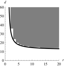
(a)   (b)  

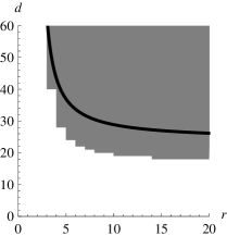
(c)   (d)  

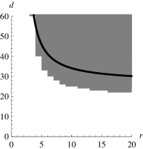
Figure 4: Sizes $(r,d)$ of creative telescoping relations together with the curve predicted by Theorem 14, for the hyperexponential terms discussed in Example 15.

     

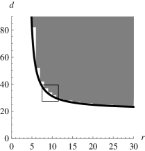
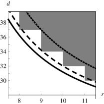
Figure 5: Left: Sizes $(r,d)$ of creative telescoping relations together with the curve predicted by Theorem 14, for the term discussed in Example 15.(5). Right: a detail of the figure on the left in a larger scale, together with the curve based on $\varphi$ instead of $\varphi^{\prime}$ (dashed) and the curve based on $w=0$ (dotted). The correct degrees are precisely the smallest integers strictly above the solid curve. The two variations both overshoot for all the points in this range.

There are several ways of refining the ansatz for $P$ and $Q$ even further in order to achieve better estimates where ours are not sharp. Here are some ideas.

• The possibility of introducing extra variables without increasing the number of equations (depicted by the white bullets in Figures 1 and 2) rests on the observation made in Lemma 9 that the leading coefficients $\operatorname{lc}_{x}N_{r,i}$ are $\mathbbm{K}$-multiples of each other, i.e., that these leading coefficients generate a linear subspace of $\mathbbm{K}[y]$ of dimension one. Experiments suggest that this observation can be generalized to the coefficients of lower degree as follows: If $V_{j}\subseteq\mathbbm{K}[y]$ denotes the vector space generated by the coefficients of $x^{\operatorname{deg}_{x}N_{r,i}-j}$ in $N_{r,i}$ ($i=0,\dots,r$), then $V_{0}\subseteq V_{1}\subseteq\cdots\subseteq V_{j}$ and $\dim V_{j}\leq j+1$ at least for small $j$. If this is true, it would allow adding more extra variables without increasing the number of equations.

• In general, comparing coefficients of the monomials $x^{i}y^{j}$ of a polynomial $S$ to zero results in a linear system with $(\operatorname{deg}_{x}S+1)(\operatorname{deg}_{y}S+1)$ equations. But if $S$ contains some factor which is free of the variables $p_{i,j}$ and $q_{i,j}$, then canceling this factor before comparing coefficients results in a system with fewer equations and the same number of variables. While in our case, it is too much to hope for a factor which would divide $S$ as a whole, it seems that at least in some cases, factors can be removed from $\operatorname{lc}_{x}S\in\mathbbm{K}[y]$ or $\operatorname{lc}_{y}S\in\mathbbm{K}[x]$. For example, when $\operatorname{deg}_{x}a>\operatorname{deg}_{x}b$ and $\operatorname{deg}_{y}a>\operatorname{deg}_{y}b$, it can be shown that $\prod_{\ell=1}^{L}\operatorname{lc}_{x}c_{\ell}\bigm{|}\operatorname{lc}_{x}S$ and $\prod_{\ell=1}^{L}\operatorname{lc}_{y}c_{\ell}\bigm{|}\operatorname{lc}_{y}S$, so $\sum_{\ell=1}^{L}\bigl{(}\operatorname{deg}_{y}\operatorname{lc}_{x}c_{\ell}+\operatorname{deg}_{x}\operatorname{lc}_{y}c_{\ell}\bigr{)}$ equations can be discarded in this case.

We have not worked out the influence of these variations in full generality, but only on some examples. It turned out that they indeed lead to tighter estimates, but the difference is rather small, and decays to zero for large $r$. At the same time, they would lead to much more complicated formulas. We do not know the reason for the gap in Examples 15.(2) and 15.(4) between the curve from Theorem 14 and the boundary of the gray region for $r\to\infty$. Even though it appears more important for a bound to be tight for small orders than for large ones, we would be very interested in seeing a refined bound which closes this gap.

It is also interesting to compare the gray regions for hyperexponential terms composed from dense random polynomials with the gray regions for hyperexponential terms of the same shape that originate from some specific application. According to our experiments, the shape of the gray region for a randomly chosen term $h=c_{0}\exp(a/b)\prod_{\ell=1}^{L}c_{\ell}^{e_{\ell}}$ only depends on the number $L$ of factors in the product, the degrees of the polynomials $a,b,c_{0},\dots,c_{L}$, and the exponents $e_{1},\dots,e_{L}$. However, input containing sparse polynomials or polynomials which in some other sense have a “structure” may well have considerably smaller degrees.

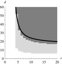
Figure 6: Gray regions for the two terms $h$ (light gray) and $g$ (dark gray) from Example 16. Although all Greek parameters have the same values for $h$ and $g$ (and hence, Theorem 14 gives the same degree estimation curve), the actual gray regions differ significantly.

Example 16.

If $a_{n,k}$ denotes the number of HC-polynomioes with $n$ cells and $k$ rows (Wilf, 1989, Section 4.9), then

$$\sum_{n,k=0}^{\infty}a_{n,k}x^{n}y^{k}=\frac{xy(1-x)^{3}}{(1-x)^{4}-xy(1-x-x^{2}+x^{3}+x^{2}y)}.$$

A differential equation for the generating function $\sum_{n=0}^{\infty}a_{n,n}x^{n}$ of the number of HC-polynomials with $n$ cells and $n$ rows can be obtained by applying creative telescoping to the rational function obtained from the rational function above by substituting $x$ by $y$, $y$ by $x/y$, and dividing the result by $y$. Let thus

$$h=\frac{1}{y}\frac{y\frac{x}{y}(1-y)^{3}}{(1-y)^{4}-y\frac{x}{y}(1-y-y^{2}+y^{3}+y^{2}\frac{x}{y})}=\frac{x(1-y)^{3}}{y((1-y)^{4}-x(1-y+xy-y^{2}+y^{3}))}.$$

Here we have $c_{0}=x(1-y)^{3}$, $a=0$, $b=1$, $c_{1}=y$, $c_{2}=((1-y)^{4}-x(1-y+xy-y^{2}+y^{3})$, $e_{1}=e_{2}=-1$. The gray region for $h$ is shown in light gray in Figure 6. For comparison, the same figure contains the gray region (in dark gray) for a term $g$ which was obtained from $h$ by replacing $c_{0}$ and $c_{2}$ by dense random polynomials with $\operatorname{deg}_{x}c_{0}=1$, $\operatorname{deg}_{y}c_{0}=3$, $\operatorname{deg}_{x}c_{2}=2$, $\operatorname{deg}_{y}c_{2}=4$, so that all the Greek parameters have precisely the same values for $g$ and $h$.

Theorem 14 predicts relations whenever $d\geq\frac{17r-2}{r-3}$ (black curve), which is a good estimate for the generic term $g$ but a significant overestimation for the special term $h$.

5 Consequences and Applications

Our theorem contains as a special case Theorem cAZ of Apagodu and Zeilberger (2006), which says that a (non-rational) hyperexponential term always admits a telescoper of order $r=\gamma+1$, but makes no statement about its degree $d$. Similarly, we can also give an estimate for the possible degrees $d$ without paying attention to their orders $r$.

Corollary 17.

1. For every hyperexponential term $h$, there exists a creative telescoping relation of order $r=\psi+1=\gamma+1-\phi_{3}$.

2. For every hyperexponential term $h$, there exists a creative telescoping relation of degree

   $$d=\vartheta+1=\left\{\begin{array}[]{ll}(\alpha+\beta)(2\gamma-1+\phi_{3})+\gamma&\quad\text{if $\operatorname{deg}_{x}a>\operatorname{deg}_{x}b$;}\\ \alpha(2\gamma-1+\phi_{3})&\quad\text{if $\operatorname{deg}_{x}a\leq\operatorname{deg}_{x}b$.}\end{array}\right.$$

Proof..

Both claims are immediate by the formulas given in Theorem 14.    $\Box$

In connecting order $r$ and degree $d$ into a single formula, Theorem 14 makes a much stronger statement than this corollary. Assuming for simplicity that the bounds of Theorem 14 are tight, we can use them to compute optimal choices for order and degree of the telescoper. There are various quantities which one may want to minimize. Besides asking for a bound on the minimal order or the minimal degree, as carried out above, we may ask for a choice $(r,d)$ where the computational cost is minimal, or the total size $S(r,d):=(r+1)(d+1)+(s_{1}+1)(\operatorname{deg}_{x}c_{0}+\gamma(r-1)+2)$ of the output (consisting of telescoper and certificate), or the size $T(r,d):=(r+1)(d+1)$ of the output telescoper alone. Or, if the telescoper $P$ is to be transformed into a recurrence for the series coefficients of its solutions, one may want to minimize the order of this recurrence, which is bounded by $R(r,d):=r+d$ (see, e.g., Thm. 7.1 in Kauers and Paule, 2011).

For minimizing the computational cost, we first have to fix a particular algorithm for computing $P$ and $Q$ for given $h$. We are not forced to follow the algorithm which is implicit in the analysis of Sections 3 and 4 (making an ansatz, comparing coefficients with respect to $x$ and $y$ to zero, and solving a linear system of equations over $\mathbbm{K}$). In fact, this algorithm has a rather poor performance. It is much better to do a coefficient comparison with respect to $y$ only and to solve a linear system of equations over $\mathbbm{K}(x)$. This is also what is proposed in the original articles (Almkvist and Zeilberger, 1990; Mohammed and Zeilberger, 2005; Apagodu and Zeilberger, 2006) and what is used in practice (Koutschan, 2009, 2010). Output sensitive linear system solvers based on Hermite-Padé approximation (Beckermann and Labahn, 1994; Storjohann and Villard, 2005; Bostan et al., 2007) are able to determine the degree $n$ solutions of a linear system over $\mathbbm{K}(x)$ with $m$ variables and at most $m$ equations using $\mathrm{O}^{\sim}(nm^{3})$ operations in $\mathbbm{K}$. Since an ansatz over $\mathbbm{K}(x)$ will have only $r+1$ variables coming from the telescoper, $\operatorname{deg}_{y}c_{0}+\gamma(r-1)-\phi_{3}+2$ variables coming from the certificate, and a solution of degree $s_{1}$ with respect to $x$, it seems reasonable to assume that the computational cost is minimal for a choice $(r,d)$ which minimizes the function $C(r,d):=s_{1}(\operatorname{deg}_{y}c_{0}+(\gamma+1)r-\gamma-\phi_{3}+3)^{3}$.

Example 18.

Consider a hyperexponential term $h=c_{0}\exp(a/b)\sqrt{c_{1}}$ where $a,b,c_{0},c_{1}\in\mathbbm{K}[x,y]$ have the degrees $\operatorname{deg}_{x}a=\operatorname{deg}_{y}a=\operatorname{deg}_{x}b=\operatorname{deg}_{y}b=1$, $\operatorname{deg}_{x}c_{0}=\operatorname{deg}_{y}c_{0}=2$, $\operatorname{deg}_{x}c_{1}=4$, $\operatorname{deg}_{y}c_{1}=6$. We are in case 2 of Theorem 14 and have $\alpha=6$, $\beta=-1$, $\gamma=8$, $\omega=4$, $\delta=5$, $\phi_{1}=0$, $\phi_{2}=0$, $\phi_{3}=0$. According to the theorem, a creative telescoping relation exists for $(r,d)$ with $r\geq 7$ and $d\geq(89r-40)/(r-6)+1=(90r-46)/(r-6)$.

On the curve $d=(90r-46)/(r-6)$, the cost function $C(r,d)=(6r+d-16)(9r-3)^{3}$ assumes its minimal value for $r=8$ rather than for the minimal order $r=7$. Finding this optimal value is easy: regard $r$ temporarily as real variable and use calculus to determine the minimum of $C(r,\tfrac{90r-46}{r-6})$. This gives a minimum point near $r=7.679$. It follows that the minimum for $r\in\mathbbm{N}$ is either at $r=7$ or at $r=8$. Comparing the actual values of $C$ at these two points indicates that the 8th order telescoper is about 8% cheaper than the 7th order operator, and hence the cheapest operator of all.

By similar calculations, we find that the output size (telescoper and certificate combined) is minimized for $r=10$, the size of the telescoper alone is minimized for $r=12$, and the order of the recurrence associated to the telescoper is minimized for $r=28$. See Figure 7 for an illustration.

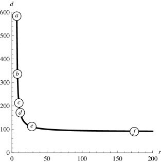
Figure 7: Points $(r,d)$ on the curve for which (a) the order, (b) the computational cost, (c) the size of telescoper and certificate combined, (d) the size of the telescoper only, (e) the order of the recurrence corresponding to the telescoper, and (f) the degree is minimal.

For the moment, the term $h$ considered in the above example is a bit too big to actually compute the creative telescoping relations of orders 7 and 8 and compare the difference of the timings to the predicted speedup of 8%. On smaller examples, the minimal (predicted) complexity is achieved for the minimal order operator. It may seem that an improvement by just a few percent is not really worth the effort. But in fact, the improvement gained in the example is just the tip of an iceberg. Asymptotically, as the input size increases, the speedup becomes more and more significant. In the next result, which is a generalization and a refinement of a result of Bostan et al. (2010), we give precise estimates.

Corollary 19.

Let $h$ be a hyperexponential term and $\tau=\max\{\alpha,\gamma,\operatorname{deg}_{x}c_{0},\operatorname{deg}_{y}c_{0}\}$. Let $\kappa$ be an increasing sublinear function with the property that degree $n$ solutions of a linear system with $m$ variables and at most $m$ equations over $\mathbbm{K}(x)$ can be computed with $nm^{3}\kappa(\max\{n,m\})$ operations in $\mathbbm{K}$. Then a creative telescoping relation of order $r=\tau-1+\phi_{3}$ can be computed using

$$2\kappa(2\tau^{3})\tau^{9}+\mathrm{O}^{\sim}(\tau^{8})$$

operations in $\mathbbm{K}$. If $r$ is chosen such that

$$r=\tfrac{1}{4}(1+\sqrt{17})\tau+\mathrm{O}(1)\leq 1.281\tau+\mathrm{O}(1)$$

then a creative telescoping relation of order $r$ can be computed using

$$\tfrac{1}{32}(349+85\sqrt{17})\kappa(11\tau^{2})\tau^{8}+\mathrm{O}(\tau^{7})\leq 21.86\kappa(11\tau^{2})\tau^{8}+\mathrm{O}^{\sim}(\tau^{7})$$

operations in $\mathbbm{K}$. In particular, creative telescoping relations for hyperexponential terms can be computed in polynomial time.

Proof..

First assume $\operatorname{deg}_{x}a>\operatorname{deg}_{x}b$. According to Theorem 14, there exists a creative telescoping relation of order $r$ and degree $d$ whenever $r\geq\tau-1+\phi_{3}$ and

$$d\geq f(r):=\frac{(2\tau^{2}+(2\beta+\phi_{3})\tau+(\phi_{3}-1)\beta)r+\mathrm{O}(\tau^{2})}{r-\tau+2-\phi_{3}},$$

where the term $\mathrm{O}(\tau^{2})$ is independent of $r$. A creative telescoping relation of order $r$ and degree $d$ can be computed using at most

$$C(r,d)=\bigl{(}(r+1)\tau+3-\phi_{3}\bigl{)}^{3}\bigl{(}(\beta+\tau)r+d-\beta(\tau+\phi_{3})-\phi_{2}-1\bigr{)}\kappa\bigl{(}(\beta+\tau)(r+1)+d\bigr{)}$$

operations in $\mathbbm{K}$. The claim follows from evaluating $C(r,f(r))$ at $r=\tau-1+\phi_{3}$ and $r=\tfrac{1}{4}(1+\sqrt{17})\tau+\mathrm{O}(1)$, respectively, and replacing the arguments of $\kappa$ by generous upper bounds.

For the case $\operatorname{deg}_{x}a\leq\operatorname{deg}_{x}b$, the estimates are proved analogously. Although the formulas for $f(r)$ and $C(r,d)$ are slightly different in this case, the final result turns out to be the same. We leave the details to the reader.    $\Box$

The strange constant $\tfrac{1}{4}(1+\sqrt{17})$ in Corollary 19 is chosen such as to minimize the multiplicative constant in the complexity bound under the simplifying assumption that $\kappa$ is constant. It was determined by first equating $\frac{d}{dr}C(r,f(r))$ to zero, which yielded the optimal choice of $r$ as an algebraic function in $\tau$, $\beta$, and $\phi_{3}$. The term $\tfrac{1}{4}(1+\sqrt{17})\tau$ is the dominant term in the asymptotic expansion of this function for $\tau\to\infty$. It is perhaps noteworthy that the choice of the constant is irrelevant for achieving a cost of $\mathrm{O}^{\sim}(\tau^{8})$, as long as the constant is greater than $1$. Taking $r=u\tau$ for arbitrary but fixed $u>1$ leads to the complexity bound $\frac{u^{4}(u+1)}{u-1}\kappa\tau^{8}+\mathrm{O}^{\sim}(\tau^{7})$. The choice $u=\tfrac{1}{4}(1+\sqrt{17})$ only minimizes the leading coefficient. Since $\tfrac{1}{4}(1+\sqrt{17})\approx 1.28$, the result indicates that when $\alpha$ and $\gamma$ are large and approximately equal, it appears to be most efficient to compute a telescoper whose order is about 30% larger than the minimum order.

In the same way as exemplified in Corollary 19, we have also determined the choices for $r$ for which some other quantities become minimal. The results are given in Table 1.

	$r$	$C(r,d)$	$S(r,d)$	$T(r,d)$	$R(r,d)$	$d$
(a)	$\tau$	$2\kappa\tau^{9}$	$\frac{2}{2-\phi_{3}}\tau^{5}$	$2\tau^{4}$	$2\tau^{3}$	$2\tau^{3}$
(b)	$\frac{1+\sqrt{17}}{4}\tau$	$\frac{349+85\sqrt{17}}{32}\kappa\tau^{8}$	$\frac{53+13\sqrt{17}}{8}\tau^{4}$	$\frac{11+3\sqrt{17}}{2}\tau^{3}$	$(5+\sqrt{17})\tau^{2}$	$(5+\sqrt{17})\tau^{2}$
(c)	$\frac{1+\sqrt{5}}{2}\tau$	$\frac{29+13\sqrt{5}}{2}\kappa\tau^{8}$	$\tfrac{11+5\sqrt{5}}{2}\tau^{4}$	$(4+2\sqrt{5})\tau^{3}$	$(3+\sqrt{5})\tau^{2}$	$(3+\sqrt{5})\tau^{2}$
(d)	$2\tau$	$48\kappa\tau^{8}$	$12\tau^{4}$	$8\tau^{3}$	$4\tau^{2}$	$4\tau^{2}$
(e)	$\sqrt{2}\tau^{3/2}$	$4\kappa\tau^{10}$	$2\tau^{5}$	$2\sqrt{2}\tau^{7/2}$	$2\tau^{2}$	$2\tau^{2}$
(f)	$2\tau^{3}$	$16\kappa\tau^{16}$	$4\tau^{8}$	$4\tau^{5}$	$2\tau^{3}$	$2\tau^{2}$

Table 1: Minimizing various functions on the curve of Theorem 14. The table shows the order $r$, the complexity $C(r,d)$, the output size $S(r,d)$ of telescoper and certificate, the output size $T(r,d)$ of the telescoper only, the recurrence order $R(r,d)$, and the degree $d$ of the telescoper when $r$ is chosen such that (a) $r$ is minimal, (b) $C(r,d)$ is minimal, (c) $S(r,d)$ is minimal, (d) $T(r,d)$ is minimal, (e) $R(r,d)$ is minimal, (f) $d$ is minimal. The parameters $\tau$ and $\kappa$ have the same meaning as in Corollary 19. The arguments of $\kappa$ are suppressed. Only the dominant terms of the asymptotic expansion for $\tau\to\infty$ are given. In rows (e) and (f), the values for $d$ differ only in the lower order terms.

As a final application, we improve some of the results given by Bostan et al. (2007) on differential and recurrence equations related to algebraic functions. Let $m\in\mathbbm{K}[x,y]$ be irreducible with $\operatorname{deg}_{y}m\geq 1$, and let $a\in\mathbbm{K}[[x]]$ be such that $m(x,a(x))=0$. According to Proposition 2 in their paper, if $P+D_{y}Q$ is a creative telescoping relation for $y(D_{y}m)/m$, then $Pa=0$. Thus we can use our results about creative telescoping to derive estimates for differential equations for $a$.

Corollary 20.

Let $m\in\mathbbm{K}[x,y]$ and $a=\sum_{n=0}^{\infty}a_{n}x^{n}\in\mathbbm{K}[[x]]$ be as above and write $\tau_{x}:=\operatorname{deg}_{x}m$, $\tau_{y}:=\operatorname{deg}_{y}m$. Assume $\tau_{x}>0$ and $\tau_{y}>0$. Then

1. The series $a$ satisfies a linear differential equation of order $r=\tau_{y}$ with coefficients of degree

   $$d=2\tau_{x}\tau_{y}^{2}-\tfrac{1}{2}\tau_{y}^{2}+\tau_{x}\tau_{y}-\tfrac{3}{2}\tau_{y}+\tau_{x}+3.$$

2. The series $a$ also satisfies a linear differential equation of order $r=2\tau_{y}$ with coefficients of degree

   $$d=4\tau_{x}\tau_{y}-\tfrac{1}{2}\tau_{y}-3\tau_{x}-1+\Bigl{\lceil}4\frac{\tau_{x}+1}{\tau_{y}+1}\Bigr{\rceil}.$$

3. The coefficient sequence $(a_{n})_{n=0}^{\infty}$ satisfies a linear recurrence equation of order

   $$\Bigl{\lceil}2\tau_{x}\tau_{y}+\tau_{y}-1+\sqrt{(8\tau_{y}^{2}-4\tau_{y}+4)\tau_{x}-2\tau_{y}^{2}-6\tau_{y}+12}\,\Bigr{\rceil}$$

   with polynomial coefficients of degree

   $$\Bigl{\lceil}\tau_{y}-1+\tfrac{1}{2}\sqrt{(8\tau_{y}^{2}-4\tau_{y}+4)\tau_{x}-2\tau_{y}^{2}-6\tau_{y}+12}\,\Bigr{\rceil}.$$

Proof..

For $h=y(D_{y}m)/m$ we have $\operatorname{deg}_{x}c_{0}\leq\alpha=\tau_{x}$, $\operatorname{deg}_{y}c_{0}=\gamma=\tau_{y}$, $\omega\leq 0$, $\delta\leq 1$, and $\phi_{3}=1$. According to Theorem 14.(2), a creative telescoping relation of order $r$ and degree $d$ exists provided that $r\geq\tau_{y}$ and

$$d\geq\frac{4\tau_{x}\tau_{y}r+2\tau_{x}\tau_{y}-\tau_{y}^{2}-3\tau_{y}+2\tau_{x}+6}{2(r-\tau_{y}+1)}.$$

Parts 1 and 2 follow from here by setting $r=\tau_{y}$ or $r=2\tau_{y}$, respectively. For part 3, observe first that there exists a creative telescoping relation of order $r$ and degree $d$ where

$$r \geq\tau_{y}-1+\tfrac{1}{2}\sqrt{(8\tau_{y}^{2}-4\tau_{y}+4)\tau_{x}-2\tau_{y}^{2}-6\tau_{y}+12},$$

$$d \geq 2\tau_{x}\tau_{y}+\tfrac{1}{2}\sqrt{(8\tau_{y}^{2}-4\tau_{y}+4)\tau_{x}-2\tau_{y}^{2}-6\tau_{y}+12}.$$

From here the claim follows by the fact that when a power series $a$ satisfies a linear differential equation of order $r$ and degree $d$, then its coefficient sequence satisfies a linear recurrence equation of order $r+d$ and degree $r$.    $\Box$

These results are to be compared with the corresponding results of Bostan et al. (degree $4\tau_{x}\tau_{y}^{2}+{}$smaller terms for part 1, order $6\tau_{y}$ and degree $3\tau_{x}\tau_{y}$ for part 2, and order and degree $2\tau_{x}\tau_{y}+\tau_{y}+1$ for part 3), as well as with the conjectures about the minimal sizes they found experimentally ($2\tau^{3}-3\tau^{2}+3\tau$ for part 1 when $\tau_{x}=\tau_{y}=:\tau$ and order and degree $2\tau_{x}\tau_{y}-2-(\tau_{x}-\tau_{y})$ for part 3 if $\tau_{y}>1$).

6 Conclusion

What is the shape of the gray region? Where does it come from? And how can it be exploited?—These were the guiding questions for the work described in this article. As a main result, we have given in Theorem 14 a simple rational function whose graph passes approximately along the boundary of the gray region, in some examples more accurately than in others. This curve was derived from a somewhat technical analysis of the linear systems resulting from a specific ansatz over $\mathbbm{K}$. Where the curve does not describe the gray region accurately, these linear systems have solutions despite of having more equations than variables. Some possible reasons for this phenomenon were taken into account in the design of the ansatz, thereby improving the accuracy of the estimate compared to a naive approach. However, as shown in Examples 15.(2) and 15.(4), there seem to be further effects which sometimes cause a gap between the true degrees and our prediction. It would be interesting to know what these effects are, and to derive sharper estimates from them. Ultimately, it would be desirable to have a version of Theorem 14 which is generically tight.

Tight curves allow for optimizing computational cost, output sizes, and other measures by trading order against degree. As the degree decreases when the order grows, it is not always optimal to compute the minimal order operator. In Example 18, we have illustrated how the curve of Theorem 14 can be used to calculate a priori the optimal orders for several interesting measures. Of course, if the curve is not tight, these predictions may not be correct, but even then, at least they provide some useful orientation. Tightness of the curve is also not required for deriving asymptotic bounds on the complexity. As we have shown in Corollary 19, the difference between the optimal choice and other choices is significant for asymptotically large input size. We believe that this result is not only of theoretical interest. Even if the minimal cost may be achieved for the minimal order in any example which is feasible with currently available hardware, it can be seen from Example 18 that it already starts to make a difference for inputs which are only slightly beyond the capability of today’s computers. We therefore expect that the technique of trading order for degree will help to optimize the performance of efficient implementations of creative telescoping in the near future.

Acknowledgements. We wish to thank Christoph Koutschan and Carsten Schneider for valuable remarks on an earlier draft of this article.

References

Abramov et al. (2004)
Abramov, S. A., Carette, J. J., Geddes, K. O., Le, H. Q., 2004. Telescoping in
the context of symbolic summation in Maple. Journal of Symbolic Computation
38 (4), 1303–1326.
Almkvist and Zeilberger (1990)
Almkvist, G., Zeilberger, D., 1990. The method of differentiating under the
integral sign. Journal of Symbolic Computation 11 (6), 571–591.
Apagodu and Zeilberger (2006)
Apagodu, M., Zeilberger, D., 2006. Multi-variable Zeilberger and
Almkvist-Zeilberger algorithms and the sharpening of Wilf-Zeilberger
theory. Advances in Applied Mathematics 37 (2), 139–152.
Beckermann and Labahn (1994)
Beckermann, B., Labahn, G., 1994. A uniform approach for the fast computation
of matrix-type Padé approximants. SIAM Journal on Matrix Analysis and
Applications 15 (3), 804–823.
Bostan et al. (2010)
Bostan, A., Chen, S., Chyzak, F., Li, Z., 2010. Complexity of creative
telescoping for bivariate rational functions. In: Proceedings of ISSAC’10.
pp. 203–210.
Bostan et al. (2007)
Bostan, A., Chyzak, F., Salvy, B., Lecerf, G., Schost, É., 2007.
Differential equations for algebraic functions. In: Proceedings of ISSAC’07.
pp. 25–32.
Bronstein et al. (2005)
Bronstein, M., Li, Z., Wu, M., 2005. Picard-vessiot extensions for linear
functional systems. In: Proceedings of ISSAC’05. pp. 68–75.
Caviness and Johnson (1998)
Caviness, B. F., Johnson, J. R. (Eds.), 1998. Quantifier Elimination and
Cylindrical Algebraic Decomposition. Texts and Monographs in Symbolic
Computation. Springer.
Christopher (1999)
Christopher, C., 1999. Liouvillian first integrals of second order polynomial
differential equations. Electronic Journal of Differential Equations
49 (#7).
Chyzak (2000)
Chyzak, F., 2000. An extension of Zeilberger’s fast algorithm to general
holonomic functions. Discrete Mathematics 217, 115–134.
Chyzak et al. (2009)
Chyzak, F., Kauers, M., Salvy, B., 2009. A non-holonomic systems approach to
special function identities. In: May, J. (Ed.), Proceedings of ISSAC’09. pp.
111–118.
Collins (1975)
Collins, G. E., 1975. Quantifier elimination for the elementary theory of real
closed fields by cylindrical algebraic decomposition. Lecture Notes in
Computer Science 33, 134–183.
Gosper (1978)
Gosper, W., 1978. Decision procedure for indefinite hypergeometric summation.
Proceedings of the National Academy of Sciences of the United States of
America 75, 40–42.
Kauers and Paule (2011)
Kauers, M., Paule, P., 2011. The Concrete Tetrahedron. Springer.
Koepf (1998)
Koepf, W., 1998. Hypergeometric Summation. Vieweg.
Koutschan (2009)
Koutschan, C., 2009. Advanced applications of the holonomic systems approach.
Ph.D. thesis, RISC-Linz, Johannes Kepler Universität Linz.
Koutschan (2010)
Koutschan, C., 2010. A fast approach to creative telescoping. Mathematics in
Computer Science 4 (2–3), 259–266.
Mohammed and Zeilberger (2005)
Mohammed, M., Zeilberger, D., 2005. Sharp upper bounds for the orders of the
recurrences outputted by the Zeilberger and q-Zeilberger algorithms.
Journal of Symbolic Computation 39 (2), 201–207.
Paule and Schorn (1995)
Paule, P., Schorn, M., 1995. A Mathematica version of Zeilberger’s
algorithm for proving binomial coefficient identities. Journal of Symbolic
Computation 20 (5–6), 673–698.
Petkovšek et al. (1997)
Petkovšek, M., Wilf, H., Zeilberger, D., 1997. . AK Peters, Ltd.
Schneider (2004)
Schneider, C., 2004. The summation package Sigma: Underlying principles and a
rhombus tiling application. Discrete Mathematics and Theoretical Computer
Science 6 (2), 365–386.
Schneider (2005)
Schneider, C., 2005. Solving parameterized linear difference equations in terms
of indefinite nested sums and products. Journal of Difference Equations and
Applications 11 (9), 799–821.
Storjohann and Villard (2005)
Storjohann, A., Villard, G., 2005. Computing the rank and a small nullspace
basis of a polynomial matrix. In: Proceedings of ISSAC’05. pp. 309–316.
Strzeboński (2000)
Strzeboński, A., 2000. Solving systems of strict polynomial inequalities.
Journal of Symbolic Computation 29, 471–480.
Strzeboński (2006)
Strzeboński, A., 2006. Cylindrical algebraic decomposition using validated
numerics. Journal of Symbolic Computation 41 (9), 1021–1038.