Multifractal analysis of multiple ergodic averages

Abstract.

In this paper we present a complete solution to the problem of multifractal analysis of multiple ergodic averages in the case of symbolic dynamics for functions of two variables depending on the first coordinate.

1. Introduction and results

Let $T:X\to X$ be a continuous map on a compact metric space $X$. Let $f_{1},\cdots,f_{\ell}$ ($\ell\geq 2$) be $\ell$ real valued continuous functions defined on $X$. We consider the following possible limits (for different $x\in X$):

(1) $$M_{f_{1},\cdots,f_{\ell}}(x)=\lim_{n\rightarrow\infty}\frac{1}{n}\sum_{k=1}^{n}f_{1}(T^{k}x)f_{2}(T^{2k}x)\cdots f_{\ell}(T^{\ell k}x).$$

Such limits are widely studied in ergodic theory. It was proposed in [2] to give a multifractal analysis of the multiple ergodic average $M_{f_{1},\cdots,f_{\ell}}(x)$. The authors of [2] succeeded in a very special case where $X=\{-1,1\}^{\mathbb{N}}$, $f_{k}(x)=x_{1}$ for all $k$ and $T$ is the shift, by using Riesz products. In this note, we shall study the shift map $T$ on the symbolic space $X=\Sigma_{m}=S^{\mathbb{N}}$ with $S=\{0,1,\cdots,m-1\}$ ($m\geq 2$). We assume that $\ell=2$ (the case $\ell\geq 3$ seems more difficult) and $f_{1}$ and $f_{2}$ are Hölder continuous. We endow $\Sigma_{m}$ with the standard metric: $d(x,y)=m^{-n}$ where $n$ is the largest $k\geq 0$ such that $x_{1}=y_{1}$, $\cdots$, $x_{k}=y_{k}$. The Hausdorff dimension of a set $A$ in $\Sigma_{m}$ will be denoted by $\dim A$.

For any $\alpha\in\mathbb{R}$, define

$$L(\alpha)=\{x\in\Sigma_{m}:M_{f_{1},f_{2}}(x)=\alpha\}.$$

Let $\alpha_{\min}=\min_{x,y\in\Sigma_{m}}f_{1}(x)f_{2}(y)$ and $\alpha_{\max}=\max_{x,y\in\Sigma_{m}}f_{1}(x)f_{2}(y)$. Our question is to determine the Hausdorff dimension of $L(\alpha)$. We further assume that $\alpha_{\min}<\alpha_{\max}$ (otherwise both $f_{1}$ and $f_{2}$ are constant and the problem is trivial).

From classical dynamical system point of view, the set $L(\alpha)$ is not standard and its dimension can not be described by invariant measures supported on it. Let us first examine the largest dimension of ergodic measures supported on the set $L(\alpha)$ by introducing the so-called invariant spectrum:

$$F_{\rm inv}(\alpha)=\sup\left\{\dim\mu:\mu\ \mbox{\rm ergodic},\mu(L(\alpha))=1\ \right\}.$$

Recall that (see [1])

$$\dim\mu=\inf\{\dim B:B\ \mbox{Borel \ set},\mu(B^{c})=0\}.$$

The dimension $F_{\rm inv}(\alpha)$ is in general smaller than $\dim L(\alpha)$ (compare the next two theorems). It is even possible that no ergodic measure is supported on $L(\alpha)$.

Theorem 1.1.

Let $f_{1}$ and $f_{2}$ be two Hölder continuous functions on $\Sigma_{m}$. If $L(\alpha)$ supports an ergodic measure, then

$$F_{\rm inv}(\alpha)=\sup\left\{\dim\mu:\mu\ \mbox{\rm ergodic},\int f_{1}d\mu\int f_{2}d\mu=\alpha\ \right\}.$$

It is known [3] that the above supremum is the dimension of the set of points $x$ such that

$$\lim_{n\to\infty}\frac{1}{n}\sum_{k=1}^{n}f_{1}(T^{k}x)\cdot\lim_{n\to\infty}\frac{1}{n}\sum_{k=1}^{n}f_{2}(T^{k}x)=\alpha.$$

Assume that $f_{1}$ and $f_{2}$ are the same function $f$. As a corollary of Theorem 1.1, $\mu(L(\alpha))=1$ for some ergodic measure $\mu$ implies $\alpha\geq 0$. So, if $f$ takes a negative value $\alpha<0$, then Theorem 1 shows that there is no ergodic measure supported on $L(\alpha)$. However, Theorem 2 shows that $\dim L(\alpha)>0$.

In the following we assume that both $f_{1}$ and $f_{2}$ depend only on the first coordinate. For any $s\in\mathbb{R}$, consider the non-linear transfer equation

(2) $$t_{s}(x)^{2}=\sum_{Ty=x}e^{sf_{1}(x)f_{2}(y)}t_{s}(y).$$

It can be proved that the equation admits a unique solution $t_{s}:\Sigma_{m}\to\mathbb{R}_{+}$, which depends only on the first coordinate. Let $dx$ denote the measure of maximal entropy for the shift on $\Sigma_{m}$ and let

$$P(s)=\log\int_{\Sigma_{m}}t_{s}(x)dx+\log m.$$

Also it can be proved that $P$ is an analytic convex function and even strictly convex when $\alpha_{\min}<\alpha_{\max}$ (Lemma 3.1).

Theorem 1.2.

Let $f_{1}$ and $f_{2}$ be two functions on $\Sigma_{m}$ depending only on the first coordinate. For $\alpha\not\in[P^{\prime}(-\infty),P^{\prime}(+\infty)]$, we have $L(\alpha)=\emptyset$. For $\alpha\in[P^{\prime}(-\infty),P^{\prime}(+\infty)]$, we have

$$\dim L(\alpha)=\frac{1}{2\log m}\left(P(s_{\alpha})-s_{\alpha}P^{\prime}(s_{\alpha})\right)$$

where $s_{\alpha}$ is the unique solution of $P^{\prime}(s)=\alpha$.

We can prove that $\alpha_{\min}\leq P^{\prime}(-\infty)\leq P^{\prime}(+\infty)\leq\alpha_{\max}$ and that $\alpha_{\min}=P^{\prime}(-\infty)$ if and only if there exist $i_{0},i_{1},\cdots,i_{\ell}\in S$ ($\ell\geq 1$) with $i_{0}=i_{\ell}$ such that $f_{1}(i_{k})f_{2}(i_{k+1})=\alpha_{\min}$ (similar criterion for $\alpha_{\max}=P^{\prime}(+\infty)$).

Let us look at two examples on $\Sigma_{2}$. For $f_{1}(x)=f_{2}(x)=2x_{1}-1$, we have

$$\dim L(\alpha)=\frac{1}{2}+\frac{1}{2}H\left(\frac{1+\alpha}{2}\right),\quad F_{\rm inv}(\alpha)=H\left(\frac{1+\sqrt{\alpha}}{2}\right)$$

where $H(x)=-x\log_{2}x-(1-x)\log_{2}(1-x)$. See Figure 1 for the graphs of $\dim L(\alpha)$ and $F_{\rm inv}(\alpha)$. Remark that $F_{\rm inv}(\alpha)=0$ but $\dim L(\alpha)>0$ for $-1\leq\alpha<0$. Also remark that $\dim L(\alpha)$ was computed in [2] by using Riesz products. See Figure 2 for the graphs of $\dim L(\alpha)$ and $F_{\rm inv}(\alpha)$ when $f_{1}(x)=f_{2}(x)=x_{1}$. In the second case $F_{\rm inv}(\alpha)=H(\sqrt{\alpha})$ and $\dim L(\alpha)$ can be numerically computed through $P(s)=2\log t_{0}(s)$ where $x=t_{0}(s)$ is the real solution of the third order algebraic equation

$$x^{3}-2x^{2}-(e^{s}-1)x+(e^{s}-1)=0.$$

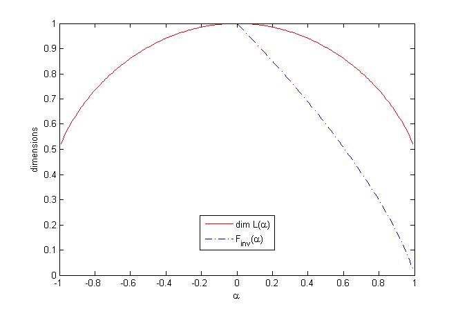
Figure 1. When $f_{1}(x)=f_{2}(x)=2x_{1}-1$.

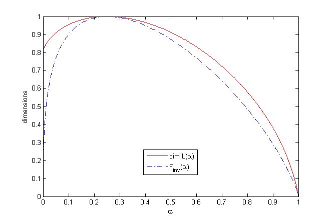
Figure 2. When $f_{1}(x)=f_{2}(x)=x_{1}$.

These two examples show that $F_{\rm inv}(\alpha)<\dim L(\alpha)$ except for some special $\alpha$’s.

The proof of Theorem 1.2 is based on the following observation. If $f_{1}$ and $f_{2}$ depend only on the first coordinate $x_{1}$, $\sum_{k}f_{1}(T^{k}x)f_{2}(T^{2k})$ can be decomposed into the sum of $\sum_{j}f_{1}(T^{i2^{j}}x)f_{2}(T^{i2^{j+1}}x)$ with odd $i$, which have independent coordinates. This observation was used in [2] to compute the box dimension of $X_{0}=\{x:\forall n,\ x_{n}x_{2n}=0\}$ which is a subset of $L(0)$ (here $f_{1}(x)=f_{2}(x)=x_{1}$ is considered). The Hausdorff dimension of $X_{0}$ was later computed in [5] where a non-linear transfer operator characterizes the measure of maximal Hausdorff dimension for $X_{0}$.

We have stated the results for functions of the form $f_{1}(x_{1})f_{2}(y_{1})$ (product of two functions depending on the first coordinate). But the results with obvious modifications hold for functions of the form $f(x_{1},y_{1})$.

2. Proof of Theorem 1.1

Let $\mu$ be an ergodic measure such that $\mu(L(\alpha))=1$. Then

$$\alpha=\lim_{n\to\infty}\frac{1}{n}\sum_{k=1}^{n}\mathbb{E}_{\mu}[f_{1}(T^{k}x)f_{2}(T^{2k}x)]=\lim_{n\to\infty}\frac{1}{n}\sum_{k=1}^{n}\mathbb{E}_{\mu}[f_{1}(x)f_{2}(T^{k}x)]=\mathbb{E}_{\mu}[f_{1}(x)M_{f_{2}}(x)].$$

(The first and third equalities are due to Lebesgue convergence theorem and the second one is due to the invariance of $\mu$). Since $\mu$ is ergodic, $M_{f_{2}}(x)=\mathbb{E}_{\mu}f_{2}$ for $\mu$-a.e. $x$. So, $\alpha=\mathbb{E}_{\mu}f_{1}\mathbb{E}_{\mu}f_{2}$. It follows that

$$F_{\rm inv}(\alpha)\leq\sup\left\{\dim\mu:\mu\ \mbox{\rm ergodic},\mathbb{E}_{\mu}f_{1}\mathbb{E}_{\mu}f_{2}=\alpha\ \right\}.$$

To obtain the inverse inequality, it suffices to observe that the above supremum is attained by a Gibbs measure $\nu$ which is mixing and that the mixing property implies $M_{f_{1},f_{2}}(x)=\mathbb{E}_{\nu}f_{1}\mathbb{E}_{\nu}f_{2}$ $\nu$-a.e..

3. Proof of Theorem 1.2

We will prove a result which is a bit more general than Theorem 1.2. Our proof is sketchy and a full proof is contained in [4] where other generalizations are also considered.

Here is the setting. Let $\varphi:S\times S\to\mathbb{R}$ be a non constant function with minimal value $\alpha_{\min}$ and maximal value $\alpha_{\max}$. For $\alpha\in\mathbb{R}$, define

$$E(\alpha)=\left\{x\in\Sigma_{m}:\lim_{n\to\infty}n^{-1}\sum_{k=1}^{n}\varphi(x_{k},x_{2k})=\alpha\right\}.$$

Lemma 3.1.

For any $s\in\mathbb{R}$, the system

$$t_{i}^{2}=\sum_{j=0}^{m-1}e^{s\varphi(i,j)}t_{j}\quad(i=0,1,\cdots,m-1)$$

admits a unique solution $(t_{0}(s),t_{1}(s),\cdots,t_{m-1}(s))$ with strictly positive components, which is an analytic function of $s$. The function

$$P(s)=\log\sum_{j=0}^{m-1}t_{j}(s)$$

is strictly convex.

The proof of the lemma is lengthy. The existence and uniqueness of the solution are based on the fact that the square roots of right members of the system define an increasing operator on a suitable compact hypercube. The analyticity of the solution is a consequence of the implicit function theorem.

Theorem 3.1.

For any $\alpha\in[P^{\prime}(-\infty),P^{\prime}(+\infty)]$, we have

$$E(\alpha)=\frac{1}{2\log m}\left(P(s_{\alpha})-s_{\alpha}P^{\prime}(s_{\alpha})\right)$$

where $s_{\alpha}$ is the unique solution of $P^{\prime}(s)=\alpha$.

The solution $(t_{0}(s),t_{1}(s),\cdots,t_{m-1}(s))$ of the above system allows us to define a Markov measure $\mu_{s}$ with initial probability $(\pi(i))_{i\in S}$ and probability transition matrix $(p_{i,j})_{S\times S}$ defined by

$$\pi(i)=\frac{t_{i}(s)}{t_{0}(s)+t_{i}(s)+\cdots+t_{m-1}(s)},\qquad p_{i,j}=e^{s\varphi(i,j)}\frac{t_{j}(s)}{t_{i}(s)^{2}}.$$

Now decompose the set of positive integers $\mathbb{N}^{*}$ into $\Lambda_{i}$ ($i$ being odd) with $\Lambda_{i}=\{i2^{k}\}_{k\geq 0}$ so that $\Sigma_{m}=\prod_{i:2\not\mid i}S^{\Lambda_{i}}$. Take a copy $\mu_{s}$ on each $S^{\Lambda_{i}}$ and then define the product measure of these copies. This gives a probability measure $\mathbb{P}_{s}$ on $\Sigma_{m}$. Let $\underline{D}(\mathbb{P}_{s},x)$ be the lower local dimension of $\mathbb{P}_{s}$ at $x$.

Lemma 3.2.

For any $x\in E(\alpha)$, we have $\underline{D}(\mathbb{P}_{s},x)\leq\frac{1}{2\log m}[P(s)-\alpha s].$

It follows that $\dim E(\alpha)\leq\frac{1}{2\log m}[P(s)-\alpha s]$. Minimizing the right hand side gives rise to

$$\dim E(\alpha)\leq\frac{1}{2\log m}[P(s_{\alpha})-\alpha s_{\alpha}]$$

where $s_{\alpha}$ is the solution of $P^{\prime}(s)=\alpha$. From the lemma, we can deduce that $L(\alpha)=\emptyset$ if $\alpha\not\in[P^{\prime}(-\infty),P^{\prime}(+\infty)]$. In order to get the inverse inequality, we only have to show that $\mathbb{P}_{s_{\alpha}}$ is supported on $L(\alpha)$. We first prove the following law of large numbers by showing the exponential correlation decay of $(F_{n})$ under $\mathbb{P}_{s}$.

Lemma 3.3.

Let $(F_{n})$ be a sequence of functions defined on $S\times S$ such that $\sup_{n}\sup_{x,y}|F_{n}(x,y)|<\infty$. For $\mathbb{P}_{s}$-a.e. $x\in\Sigma_{m}$, we have

$$\lim_{n\to\infty}\frac{1}{n}\sum_{k=1}^{n}\left(F_{k}(x_{k},x_{2k})-\mathbb{E}_{\mathbb{P}_{s}}F_{k}(x_{k},x_{2k})\right)=0.$$

Applying the above lemma to $F_{n}(x_{n},x_{2n})=\varphi(x_{n},x_{2n})$ for all $n$ and computing $\mathbb{E}_{\mathbb{P}_{s}}\varphi(x_{n},x_{2n})$, we get

Lemma 3.4.

For $\mathbb{P}_{s}$-a.e. $x\in\Sigma_{m}$, we have

$$\lim_{n\to\infty}\frac{1}{n}\sum_{k=1}^{n}\varphi(x_{k},x_{2k})=P^{\prime}(s).$$

Thus we finished the proof for $\alpha\in(P^{\prime}(-\infty),P^{\prime}(+\infty))$. If $\alpha=P^{\prime}(-\infty)$ (resp. $P^{\prime}(+\infty)$), as in the standard multifractal analysis, we use the probabilities $\mathbb{P}_{s}$ et let $s$ tend to $-\infty$ (resp. $+\infty$).

Acknowledgement The author would like to thank B. Solomyak for his careful reading of the note and for the information that the Hausdorff dimension of $L(\alpha)$ is computed in a different way for the special case $m=2,f_{1}(x)=f_{2}(x)=x_{1}$ in [6].

References

[1] A.H. Fan Sur les dimension de measure, Studia Math., 111 (1994), 1-17.
[2] A.H. Fan, L. M. Liao and J. H. Ma Level sets of multiple ergodic averages. preprint, 2009.
[3] A.H. Fan, L. M. Liao and J. Peyrière Generic points in systems of specification and Banach
valued Birkhff ergodic average, DCDS, 21 (2008), 1103-1128.
[4] A.H. Fan, J. Schmeling and M. Wu, Multiple ergodic averages and nonlinear transfer operaters. preprint, 2011.
[5] R. Kenyon, Y. Peres and B. Solomyak, Hausdorff dimension for fractals invariant
under the multiplicative integers. preprint, 2011.
[6] Y. Peres and B. Solomyak, Dimension spectrum for a nonconventional ergodic average. preprint, 2011.