Supplement paper to “Online Expectation Maximization based algorithms for inference in Hidden Markov Models”

This is a supplementary material to the paper [7].

It contains technical discussions and/or results adapted from published papers. In Sections 2 and 3, we provide results - useful for the proofs of some theorems in [7] - which are close to existing results in the literature.

It also contains, in Section 4, additional plots for the numerical analyses in [7, Section $3$].

To make this supplement paper as self-contained as possible, we decided to rewrite in Section 1 the model and the main definitions introduced in [7].

1 Assumptions and Model

Our model is defined as follows. Let $\Theta$ be a compact subset of $\mathbb{R}^{d_{\theta}}$. We are given a family of transition kernels $\{M_{\theta}\}_{\theta\in\Theta}$, $M_{\theta}:\mathbb{X}\times\mathcal{X}\to[0,1]$, a positive $\sigma$-finite measure $\mu$ on $(\mathbb{Y},\mathcal{Y})$, and a family of transition densities with respect to $\mu$, $\{g_{\theta}\}_{\theta\in\Theta}$, $g_{\theta}:\mathbb{X}\times\mathbb{Y}\to\mathbb{R}_{+}$. It is assumed that, for any $\theta\in\Theta$ and any $x\in\mathbb{X}$, $M_{\theta}(x,\cdot)$ has a density $m_{\theta}(x,\cdot)$ with respect to a finite measure $\lambda$ on $(\mathbb{X},\mathcal{X})$. In the setting of this paper, we consider a single observation path $\mathbf{Y}\stackrel{{\scriptstyle\mathrm{def}}}{{=}}\{Y_{t}\}_{t\in\mathbb{Z}}$ defined on the probability space $\left(\Omega,\mathcal{F},\mathbb{P}\right)$ and taking values in $\mathbb{Y}^{\mathbb{Z}}$. The following assumptions are assumed to hold.

• 1. There exist continuous functions $\phi:\Theta\to\mathbb{R}$, $\psi:\Theta\to\mathbb{R}^{d}$ and $S:\mathbb{X}\times\mathbb{X}\times\mathbb{Y}\to\mathbb{R}^{d}$ s.t.

     $$\log m_{\theta}(x,x^{\prime})+\log g_{\theta}(x^{\prime},y)=\phi(\theta)+\left\langle S(x,x,^{\prime},y),\psi(\theta)\right\rangle\;,$$

     where $\left\langle\cdot,\cdot\right\rangle$ denotes the scalar product on $\mathbb{R}^{d}$.

  2. There exists an open subset $\mathcal{S}$ of $\mathbb{R}^{d}$ that contains the convex hull of $S(\mathbb{X}\times\mathbb{X}\times\mathbb{Y})$.

  3. There exists a continuous function $\bar{\theta}:\mathcal{S}\to\Theta$ s.t. for any $s\in\mathcal{S}$,

     $$\bar{\theta}(s)=\mathrm{argmax}_{\theta\in\Theta}\;\left\{\phi(\theta)+\left\langle s,\psi(\theta)\right\rangle\right\}\;.$$

• There exist $\sigma_{-}$ and $\sigma_{+}$ s.t. for any $\left(x,x^{\prime}\right)\in\mathbb{X}^{2}$ and any $\theta\in\Theta$, $0<\sigma_{-}\leq m_{\theta}(x,x^{\prime})\leq\sigma_{+}$. Set $\rho\stackrel{{\scriptstyle\mathrm{def}}}{{=}}1-(\sigma_{-}/\sigma_{+})\;.$

We now introduce assumptions on the observation process. For any sequence of r.v. $Z\stackrel{{\scriptstyle\mathrm{def}}}{{=}}\{Z_{t}\}_{t\in\mathbb{Z}}$ on $(\Omega,\mathbb{P},\mathcal{F})$, let

$$\mathcal{F}_{k}^{Z}\stackrel{{\scriptstyle\mathrm{def}}}{{=}}\sigma\left(\{Z_{u}\}_{u\leq k}\right)\quad\mbox{and}\quad\mathcal{G}_{k}^{Z}\stackrel{{\scriptstyle\mathrm{def}}}{{=}}\sigma\left(\{Z_{u}\}_{u\geq k}\right)$$

be $\sigma$-fields associated to $Z$. We also define the mixing coefficients by, see [4],

$$\beta^{\mathbf{Y}}(n)=\underset{u\in\mathbb{Z}}{\sup}\,\underset{B\in\mathcal{G}_{u+n}^{\mathbf{Y}}}{\sup}\,\mathbb{E}\left[|\mathbb{P}(B|\mathcal{F}_{u}^{\mathbf{Y}})-\mathbb{P}(B)|\right]\;,\forall\;n\geq 0\;.$$ (1)

• -($p$) $\mathbb{E}\left[\sup_{x,x^{\prime}\in\mathbb{X}^{2}}\,|S(x,x^{\prime},\mathbf{Y}_{0})|^{p}\right]<+\infty$.

• 1. $\mathbf{Y}$ is a $\beta$-mixing stationary sequence such that there exist $C\in[0,1)$ and $\beta\in(0,1)$ satisfying, for any $n\geq 0$, $\beta^{\mathbf{Y}}(n)\leq C\beta^{n}$, where $\beta^{\mathbf{Y}}$ is defined in (1).

  2. $\mathbb{E}\left[|\log b_{-}(\mathbf{Y}_{0})|+|\log b_{+}(\mathbf{Y}_{0})|\right]<+\infty$ where

     $$b_{-}(y) \stackrel{{\scriptstyle\mathrm{def}}}{{=}}\inf_{\theta\in\Theta}\int g_{\theta}(x,y)\lambda(\mathrm{d}x)\;,$$ (2)

     $$b_{+}(y) \stackrel{{\scriptstyle\mathrm{def}}}{{=}}\sup_{\theta\in\Theta}\int g_{\theta}(x,y)\lambda(\mathrm{d}x)\;.$$ (3)

• There exists $c>0$ and $a>1$ such that for all $n\geq 1$, $\tau_{n}=\lfloor cn^{a}\rfloor$.

Recall the following definition from [7]: for a distribution $\chi$ on $(\mathbb{X},\mathcal{B}(\mathbb{X}))$, positive integers $T,\tau$ and $\theta\in\Theta$, set

$$\bar{S}_{\tau}^{\chi,T}(\theta,\mathbf{Y})\stackrel{{\scriptstyle\mathrm{def}}}{{=}}\frac{1}{\tau}\sum_{t=T+1}^{T+\tau}\Phi_{\theta,t,T+\tau}^{\chi,T}\left(S,\mathbf{Y}\right)\;,$$ (4)

where $S$ is the function given by HH1(a) and

$$\Phi_{\theta,s,t}^{\chi,r}(S,\mathbf{y})\\ \stackrel{{\scriptstyle\mathrm{def}}}{{=}}\frac{\int\chi(\mathrm{d}x_{r})\{\prod_{i=r}^{t-1}m_{\theta}(x_{i},x_{i+1})g_{\theta}(x_{i+1},y_{i+1})\}\,S(x_{s-1},x_{s},y_{s})\,\lambda(\mathrm{d}x_{r+1:t})}{\int\chi(\mathrm{d}x_{r})\{\prod_{i=r}^{t-1}m_{\theta}(x_{i},x_{i+1})g_{\theta}(x_{i+1},y_{i+1})\}\,\lambda(\mathrm{d}x_{r+1:t})}\;.$$ (5)

We also write $S_{n-1}\stackrel{{\scriptstyle\mathrm{def}}}{{=}}\bar{S}_{\tau_{n}}^{\chi_{n-1},T_{n-1}}(\theta_{n-1},\mathbf{Y})$ the intermediate quantity computed by the BOEM algorithm in block $n$ and $\widetilde{S}_{n-1}$ the associated Monte Carlo approximation.

• -($p$) There exists $b\geq(a+1)/2a$ (where $a$ is defined in HH5) such that, for any $n\geq 0$,

  $$\left\|S_{n}-\widetilde{S}_{n}\right\|_{p}=O(\tau_{n+1}^{-b})\;,$$

  where $\widetilde{S}_{n}$ is the Monte Carlo approximation of $S_{n}$.

Define for any $\theta\in\Theta$,

$$\bar{\mathrm{S}}(\theta)\stackrel{{\scriptstyle\mathrm{def}}}{{=}}\mathbb{E}\left[\mathsf{S}(\theta,\mathbf{Y})\right]\;.$$ (6)

$$\mathrm{R}(\theta)\stackrel{{\scriptstyle\mathrm{def}}}{{=}}\bar{\theta}\left(\bar{\mathrm{S}}(\theta)\right)\;.$$ (7)

$$\mathrm{G}(s)\stackrel{{\scriptstyle\mathrm{def}}}{{=}}\bar{\mathrm{S}}(\bar{\theta}(s))\;,\qquad\forall s\in\mathcal{S}\;,$$ (8)

where $\bar{\theta}$ is given by HH1(c).

• 1. $\bar{\mathrm{S}}$ and $\bar{\theta}$ are twice continuously differentiable on $\Theta$ and $\mathcal{S}$.

  2. There exists $0<\gamma<1$ s.t. the spectral radius of $\nabla_{s}(\bar{\mathrm{S}}\circ\bar{\theta})_{s=\bar{\mathrm{S}}(\theta_{\star})}$ is lower than $\gamma$.

Set

$$T_{n}\stackrel{{\scriptstyle\mathrm{def}}}{{=}}\sum_{i=1}^{n}\tau_{i}\;,\qquad T_{0}\stackrel{{\scriptstyle\mathrm{def}}}{{=}}0\;.$$

2 Detailed proofs of [7]

2.1 Proof of [7, Theorem $4.4$]

Proof.

By [7, Proposition A.$1$], it is sufficient to prove that

$$\left|\mathrm{W}\circ\mathrm{R}(\theta_{n})-\mathrm{W}\circ\bar{\theta}(\widetilde{S}_{n})\right|\underset{n\to+\infty}{\longrightarrow}0\;,\quad\mathbb{P}\mathrm{-a.s.}\;.$$ (9)

By Theorem $4.1$, the function $\bar{\mathrm{S}}$ given by (6) is continuous on $\Theta$ and then $\bar{\mathrm{S}}(\Theta)\stackrel{{\scriptstyle\mathrm{def}}}{{=}}\{s\in\mathcal{S};\exists\theta\in\Theta,s=\bar{\mathrm{S}}(\theta)\}$ is compact and, for any $\delta>0$, we can define the compact subset $\bar{\mathrm{S}}(\Theta,\delta)\stackrel{{\scriptstyle\mathrm{def}}}{{=}}\left\{s\in\mathbb{R}^{d};\mathrm{d}(s,\bar{\mathrm{S}}(\Theta))\leq\delta\right\}$ of $\mathcal{S}$, where $\mathrm{d}(s,\bar{\mathrm{S}}(\Theta))\stackrel{{\scriptstyle\mathrm{def}}}{{=}}\inf_{s^{\prime}\in\bar{\mathrm{S}}(\Theta)}\left|s-s^{\prime}\right|$. Let $\delta>0$ (small enough) and $\varepsilon>0$. Since $\mathrm{W}\circ\bar{\theta}$ is continuous (see HH1(c) and [7, Proposition $4.2$]) and $\bar{\mathrm{S}}(\Theta,\delta)$ is compact, $\mathrm{W}\circ\bar{\theta}$ is uniformly continuous on $\bar{\mathrm{S}}(\Theta,\delta)$ and there exists $\eta>0$ s.t.,

$$\forall x,y\in\bar{\mathrm{S}}(\Theta,\delta)\;,\quad|x-y|\leq\eta\Rightarrow|\mathrm{W}\circ\bar{\theta}(x)-\mathrm{W}\circ\bar{\theta}(y)|\leq\varepsilon\;.$$ (10)

Set $\alpha\stackrel{{\scriptstyle\mathrm{def}}}{{=}}\delta\wedge\eta$ and $\Delta S_{n}\stackrel{{\scriptstyle\mathrm{def}}}{{=}}|\bar{\mathrm{S}}(\theta_{n})-\widetilde{S}_{n}|$. We write,

$$\mathbb{P}\left\{\left|\mathrm{W}\circ\bar{\theta}(\bar{\mathrm{S}}(\theta_{n}))-\mathrm{W}\circ\bar{\theta}(\widetilde{S}_{n})\right|\geq\varepsilon\right\}$$

$$=\mathbb{P}\left\{\left|\mathrm{W}\circ\bar{\theta}(\bar{\mathrm{S}}(\theta_{n}))-\mathrm{W}\circ\bar{\theta}(\widetilde{S}_{n})\right|\geq\varepsilon;\Delta S_{n}>\delta\right\}$$

$$+\mathbb{P}\left\{\left|\mathrm{W}\circ\bar{\theta}(\bar{\mathrm{S}}(\theta_{n}))-\mathrm{W}\circ\bar{\theta}(\widetilde{S}_{n})\right|\geq\varepsilon;\Delta S_{n}\leq\delta\right\}$$

$$\leq\mathbb{P}\left\{\Delta S_{n}>\delta\right\}+\mathbb{P}\left\{\Delta S_{n}>\eta\right\}\leq 2\mathbb{P}\left\{\Delta S_{n}>\alpha\right\}\;.$$

By the Markov inequality and [7, Theorem $4.1$], for all $p\in(2,\bar{p})$, there exists a constant $C$ s.t.

$$\mathbb{P}\left\{\left|\mathrm{W}\circ\bar{\theta}(\bar{\mathrm{S}}(\theta_{n}))-\mathrm{W}\circ\bar{\theta}(\widetilde{S}_{n})\right|\geq\varepsilon\right\}\leq\frac{2}{\alpha^{p}}\mathbb{E}\left[|\bar{\mathrm{S}}(\theta_{n})-\widetilde{S}_{n}|^{p}\right]\leq C\tau_{n+1}^{-p/2}\;.$$

(9) follows from HH5 and the Borel-Cantelli lemma (since $p>2$ and $a>1$). ∎

Proposition 2.1 shows that we can address equivalently the convergence of the statistics $\{\widetilde{S}_{n}\}_{n\geq 0}$ to some fixed point of $\mathrm{G}$ and the convergence of the sequence $\{\theta_{n}\}_{n\geq 0}$ to some fixed point of $\mathrm{R}$.

Proposition 2.1.

Assume HH1-H2, HH3-($\bar{p}$), HH4(a), HH5 and HH6-($\bar{p}$) for some $\bar{p}>2$.

1. Let $\theta_{\star}\in\mathcal{L}$. Set $s_{\star}\stackrel{{\scriptstyle\mathrm{def}}}{{=}}\bar{\mathrm{S}}(\theta_{\star})=\mathrm{G}(s_{\star})$. Then, $\mathbb{P}\mathrm{-a.s.}$,

   $$\underset{n\to+\infty}{\lim}\left|\widetilde{S}_{n}-s_{\star}\right|\mathbf{1}_{\lim_{n}\theta_{n}=\theta_{\star}}=0\;.$$

2. Let $s_{\star}\in\mathcal{S}$ s.t. $\mathrm{G}(s_{\star})=s_{\star}$. Set $\theta_{\star}\stackrel{{\scriptstyle\mathrm{def}}}{{=}}\bar{\theta}(s_{\star})=\mathrm{R}(\theta_{\star})$. Then $\mathbb{P}\mathrm{-a.s.}$,

   $$\underset{n\to+\infty}{\lim}\left|\theta_{n}-\theta_{\star}\right|\mathbf{1}_{\lim_{n}\widetilde{S}_{n}=s_{\star}}=0\;.$$

Proof.

Let $\bar{\mathrm{S}}$ be given by (6). By [7, Theorem $4.1$] and HH5,

$$\lim_{n}\left(\widetilde{S}_{n}-\bar{\mathrm{S}}(\theta_{n})\right)=0\quad\mathbb{P}\mathrm{-a.s.}$$

By [7, Theorem $4.1$], $\bar{\mathrm{S}}$ is continuous. Hence,

$$\lim_{n}\left|\widetilde{S}_{n}-\bar{\mathrm{S}}(\theta_{\star})\right|\mathbf{1}_{\lim_{n}\theta_{n}=\theta_{\star}}=0\quad\mathbb{P}\mathrm{-a.s.}$$

and the proof of (i) follows. Since $\bar{\theta}$ is continuous, (ii) follows. ∎

2.2 Proof of [7, Proposition $6.2$]

We start with rewriting some definitions and assumptions introduced in [7]. Define the sequences $\mu_{n}$ and $\rho_{n}$, $n\geq 0$ by $\mu_{0}=0$, $\rho_{0}=\widetilde{S}_{0}-s_{\star}$ and

$$\mu_{n}\stackrel{{\scriptstyle\mathrm{def}}}{{=}}\Gamma\mu_{n-1}+e_{n}\;,\qquad\rho_{n}\stackrel{{\scriptstyle\mathrm{def}}}{{=}}\widetilde{S}_{n}-s_{\star}-\mu_{n}\;,\qquad n\geq 1\;,$$ (11)

where, $\Gamma\stackrel{{\scriptstyle\mathrm{def}}}{{=}}\nabla\mathrm{G}(s_{\star})$,

$$e_{n}\stackrel{{\scriptstyle\mathrm{def}}}{{=}}\widetilde{S}_{n}-\bar{\mathrm{S}}(\theta_{n})\;,\qquad n\geq 1\;,$$ (12)

and $\bar{\mathrm{S}}$ is given by (6).

Proof.

Let $p\in(2,\bar{p})$. By (11), for all $n\geq 1$, $\mu_{n}=\sum_{k=0}^{n-1}\Gamma^{k}e_{n-k}$. By HH7 and the Minkowski inequality, for all $n\geq 1$, $\left\|\mu_{n}\right\|_{p}\leq\sum_{k=0}^{n-1}\gamma^{k}\left\|e_{n-k}\right\|_{p}$. By [7, Theorem $4.1$], there exists a constant $C$ s.t. for any $n\geq 1$,

$$\left\|\mu_{n}\right\|_{p}\leq C\sum_{k=0}^{n-1}\gamma^{k}\sqrt{\frac{1}{\tau_{n+1-k}}}\;.$$

By [8, Result 178, p. 39] and HH5, this yields $\sqrt{\tau_{n}}\mu_{n}=O_{\mathrm{L}_{p}}(1)$.

By HH7, using a Taylor expansion with integral form of the remainder term,

$$\mathrm{G}(\widetilde{S}_{n-1})-\mathrm{G}(s_{\star}) -\Gamma\left(\widetilde{S}_{n-1}-s_{\star}\right)$$

$$=\sum_{i,j=1}^{d}\left(\widetilde{S}_{n-1,i}-s_{\star,i}\right)\left(\widetilde{S}_{n-1,j}-s_{\star,j}\right)R_{n-1}(i,j)$$

$$=\sum_{i,j=1}^{d}(\mu_{n-1,i}+\rho_{n-1,i})(\mu_{n-1,j}+\rho_{n-1,j})R_{n-1}(i,j)\;,$$

where $x_{n,i}$ denotes the $i$-th component of $x_{n}\in\mathbb{R}^{d}$ and

$$R_{n}(i,j)\stackrel{{\scriptstyle\mathrm{def}}}{{=}}\int_{0}^{1}(1-t)\frac{\partial^{2}\mathrm{G}}{\partial s_{i}\partial s_{j}}\left(s_{\star}+t(\widetilde{S}_{n}-s_{\star})\right)\mathrm{d}t\;,\qquad n\in\mathbb{N},1\leq i,j\leq d\;.$$

Observe that under HH7, $\limsup_{n}|R_{n}|\mathbf{1}_{\lim_{n}\theta_{n}=\theta_{\star}}<\infty$ w.p.1. Define for $n\geq 1$ and $k\leq n$,

$$H_{n} \stackrel{{\scriptstyle\mathrm{def}}}{{=}}\sum_{i=1}^{d}(2\mu_{n,i}+\rho_{n,i})R_{n}(i,\cdot)\;,\quad r_{n}\stackrel{{\scriptstyle\mathrm{def}}}{{=}}\sum_{i,j=1}^{d}R_{n}(i,j)\mu_{n,i}\mu_{n,j}\;,$$ (13)

$$\psi(n,k) \stackrel{{\scriptstyle\mathrm{def}}}{{=}}(\Gamma+H_{n})\cdots(\Gamma+H_{k})\;,$$ (14)

with the convention $\psi(n,n+1)\stackrel{{\scriptstyle\mathrm{def}}}{{=}}\mathrm{Id}$. By (11),

$$\rho_{n}=\psi(n-1,0)\rho_{0}+\sum_{k=0}^{n-1}\psi(n-1,k+1)r_{k}\;.$$ (15)

Since $\sqrt{\tau_{n}}\mu_{n}=O_{\mathrm{L}_{p}}(1)$, HH5 and $p>2$ imply that $\mu_{n}\underset{n\to+\infty}{\longrightarrow}0$, $\mathbb{P}\mathrm{-a.s.}$ Then, by (11), $\rho_{n}\mathbf{1}_{\lim_{n}\theta_{n}=\theta_{\star}}\underset{n\to+\infty}{\longrightarrow}0$, $\mathbb{P}\mathrm{-a.s.}$ and by (13) $\underset{n\to+\infty}{\lim}\left|H_{n}\right|\mathbf{1}_{\lim_{n}\theta_{n}=\theta_{\star}}=0$, $\mathbb{P}\mathrm{-a.s.}$ Let $\widetilde{\gamma}\in(\gamma,1)$, where $\gamma$ is given by HH7. Since $\underset{n\to+\infty}{\lim}\left|H_{n}\right|\mathbf{1}_{\lim_{n}\theta_{n}=\theta_{\star}}=0$, there exists a $\mathbb{P}\mathrm{-a.s.}$ finite random variable $Z_{1}$ s.t., for all $0\leq k\leq n-1$,

$$\left|\psi(n-1,k)\right|\mathbf{1}_{\lim_{n}\theta_{n}=\theta_{\star}}\leq\widetilde{\gamma}^{n-k}Z_{1}\mathbf{1}_{\lim_{n}\theta_{n}=\theta_{\star}}\;.$$ (16)

Therefore, $\left|\psi(n-1,0)\rho_{0}\right|\mathbf{1}_{\lim_{n}\theta_{n}=\theta_{\star}}\leq\widetilde{\gamma}^{n}Z_{1}\,\left|\rho_{0}\right|\quad\mathbb{P}\mathrm{-a.s.}$, and, by HH3-($\bar{p}$), (4), (5), $\mathbb{E}\left[|\rho_{0}|^{\bar{p}}\right]<+\infty$ which implies that $\rho_{0}<+\infty$ $\mathbb{P}\mathrm{-a.s.}$ Since $\widetilde{\gamma}<1$, the first term in the RHS of (15) is $\tau_{n}^{-1}O_{\mathrm{L}_{p}}(1)O_{\mathrm{a.s}}(1)$.

We now consider the second term in the RHS of (15). From equation (16),

$$\left|\sum_{k=0}^{n-1}\psi(n-1,k+1)r_{k}\right|\mathbf{1}_{\lim_{n}\theta_{n}=\theta_{\star}}\leq Z_{1}\;\sum_{k=0}^{n-1}\widetilde{\gamma}^{n-k-1}\left|r_{k}\right|\mathbf{1}_{\lim_{n}S_{n}=s_{\star}}\;,\quad\mathbb{P}\mathrm{-a.s.}$$

By (13) and HH7, there exists a $\mathbb{P}\mathrm{-a.s.}$ finite random variable $Z_{2}$ s.t.

$$\left|r_{k}\right|\mathbf{1}_{\lim_{n}\theta_{n}=\theta_{\star}}\leq Z_{2}\sum_{i,j=1}^{d}\mu_{k,i}\mu_{k,j}\;,\quad\mathbb{P}\mathrm{-a.s.}$$

In addition, since $\sqrt{\tau_{n}}\mu_{n}=O_{\mathrm{L}_{p}}(1)$, there exists a constant $C$ s.t.

$$\left\|\sum_{k=0}^{n-1}\widetilde{\gamma}^{n-k-1}\sum_{i,j=1}^{d}\mu_{k,i}\mu_{k,j}\right\|_{p/2}\leq C\;\sum_{k=0}^{n-1}\frac{\widetilde{\gamma}^{n-k-1}}{\tau_{k}}\;.$$

Applying again [8, Result 178, p. 39] yields that the second term in the RHS of (15) is $\tau_{n}^{-1}O_{\mathrm{a.s}}(1)O_{\mathrm{L}_{p/2}}(1)$. ∎

3 General results on HMM

In this section, we derive results on the forgetting properties of HMM (Section 3.1), on their applications to bivariate smoothing distributions (Section 3.2), on the asymptotic behavior of the normalized log-likelihood (Section 3.3) and on the normalized score (Section 3.4).

For any sequence $\mathbf{y}\in\mathbb{Y}^{\mathbb{Z}}$ and any function $h:\mathbb{X}^{2}\times\mathbb{Y}\to\mathbb{R}$, denote by $h_{s}$ the function on $\mathbb{X}^{2}\to\mathbb{R}$ given by

$$h_{s}(x,x^{\prime})\stackrel{{\scriptstyle\mathrm{def}}}{{=}}h(x,x^{\prime},y_{s})\;.$$ (17)

3.1 Forward and Backward forgetting

In this section, the dependence on $\theta$ is dropped from the notation for better clarity. For any $s\in\mathbb{Z}$ and any $A\in\mathcal{X}$, define

$$L_{s}(x,A)\stackrel{{\scriptstyle\mathrm{def}}}{{=}}\int m(x,x^{\prime})g(x^{\prime},y_{s+1})\mathbf{1}_{A}(x^{\prime})\lambda(\mathrm{d}x^{\prime})\;,$$ (18)

and, for any $s\leq t$ denote by $L_{s:t}$ the composition of the kernels defined by

$$L_{s:s}\stackrel{{\scriptstyle\mathrm{def}}}{{=}}L_{s}\;,\qquad L_{s:u+1}(x,A)\stackrel{{\scriptstyle\mathrm{def}}}{{=}}\int L_{s:u}(x,\mathrm{d}x^{\prime})L_{u+1}(x^{\prime},A)\;.$$

By convention, $L_{s:s-1}$ is the identity kernel: $L_{s:s-1}(x,A)=\delta_{x}(A)$. For any $\mathbf{y}\in\mathbb{Y}^{\mathbb{Z}}$, any probability distribution $\chi$ on $\left(\mathbb{X},\mathcal{X}\right)$ and for any integers such that $r\leq s<t$, let us define two Markov kernels on $(\mathbb{X},\mathcal{X})$ by

$$\mathrm{F}_{s,t}(x,A) \stackrel{{\scriptstyle\mathrm{def}}}{{=}}\frac{\int L_{s}(x,\mathrm{d}x_{s+1})1_{A}(x_{s+1})L_{s+1:t-1}(x_{s+1},\mathbb{X})}{L_{s:t-1}(x,\mathbb{X})}\;,$$ (19)

$$\mathrm{B}_{s}^{\chi,r}(x,A) \stackrel{{\scriptstyle\mathrm{def}}}{{=}}\frac{\int\phi_{s|r:s}^{\chi,r}(\mathrm{d}x_{s})1_{A}(x_{s})m(x_{s},x)}{\int\phi_{s|r:s}^{\chi,r}(\mathrm{d}x_{s})m(x_{s},x)}\;,$$ (20)

where

$$\phi_{s|r:s}^{\chi,r}(A)\stackrel{{\scriptstyle\mathrm{def}}}{{=}}\frac{\int\chi(\mathrm{d}x_{r})L_{r:s-1}(x_{r},\mathrm{d}x_{s})1_{A}(x_{s})}{\int\chi(\mathrm{d}x_{r})L_{r:s-1}(x_{r},\mathbb{X})}\;.$$

Finally, the Dobrushin coefficient of a Markov kernel $F:\left(\mathbb{X},\mathcal{X}\right)\longrightarrow[0,1]$ is defined by:

$$\delta(F)\stackrel{{\scriptstyle\mathrm{def}}}{{=}}\frac{1}{2}\underset{\left(x,x^{\prime}\right)\in\mathbb{X}^{2}}{\sup}\left|\left|F(x,\cdot)-F(x^{\prime},\cdot)\right|\right|_{\mathrm{TV}}\;.$$

Lemma 3.1.

Assume that there exist positive numbers $\sigma_{-},\sigma_{+}$ such that $\sigma_{-}\leq m(x,x^{\prime})\leq\sigma_{+}$ for any $x,x^{\prime}\in\mathbb{X}$. Then for any $\mathbf{y}\in\mathbb{Y}^{\mathbb{Z}}$, $\delta(\mathrm{F}_{s,t})\leq\rho$ and $\delta(\mathrm{B}_{s}^{\chi,r})\leq\rho$ where $\rho\stackrel{{\scriptstyle\mathrm{def}}}{{=}}\sigma_{-}/\sigma_{+}$.

Proof.

Let $r$, $s$, $t$ be such that $r\leq s<t$. Under the stated assumptions,

$$\int L_{s}(x_{s},\mathrm{d}x_{s+1})1_{A}(x_{s+1})L_{s+1:t-1}(x_{s+1},\mathbb{X})\\ \geq\sigma_{-}\int g(x_{s+1},y_{s+1})1_{A}(x_{s+1})L_{s+1:t-1}(x_{s+1},\mathbb{X})\lambda(\mathrm{d}x_{s+1})$$

and

$$L_{s:t-1}(x_{s},\mathbb{X})\leq\sigma_{+}\int g(x_{s+1},y_{s+1})L_{s+1:t-1}(x_{s+1},\mathbb{X})\lambda(\mathrm{d}x_{s+1})\;.$$

This yields to

$$\mathrm{F}_{s,t}(x_{s},A)\geq\frac{\sigma_{-}}{\sigma_{+}}\frac{\int g(x_{s+1},y_{s+1})L_{s+1:t-1}(x_{s+1},\mathbb{X})\mathbf{1}_{A}(x_{s+1})\lambda(\mathrm{d}x_{s+1})}{\int g(x_{s+1},y_{s+1})L_{s+1:t-1}(x_{s+1},\mathbb{X})\lambda(\mathrm{d}x_{s+1})}\;.$$

Similarly, the assumption implies

$$\mathrm{B}_{s}^{\chi,r}(x_{s+1},A)\geq\frac{\sigma_{-}}{\sigma_{+}}\phi_{s|r:s}^{\chi,r}(A)\;,$$

which gives the upper bound for the Dobrushin coefficients, see [3, Lemma 4.3.13]. ∎

Lemma 3.2.

Assume that there exist positive numbers $\sigma_{-},\sigma_{+}$ such that $\sigma_{-}\leq m(x,x^{\prime})\leq\sigma_{+}$ for any $x,x^{\prime}\in\mathbb{X}$. Let $\mathbf{y}\in\mathbb{Y}^{\mathbb{Z}}$.

1. for any bounded function $h$, any probability distributions $\chi$ and $\widetilde{\chi}$ and any integers $r\leq s\leq t$

   $$\left|\frac{\int\chi(\mathrm{d}x_{r})L_{r:s-1}(x_{r},\mathrm{d}x_{s})h(x_{s})L_{s:t-1}(x_{s},\mathbb{X})}{\int\chi(\mathrm{d}x_{r})L_{r:t-1}(x_{r},\mathbb{X})}\right.\\ \hskip 28.45274pt\left.-\frac{\int\widetilde{\chi}(\mathrm{d}x_{r})L_{r:s-1}(x_{r},\mathrm{d}x_{s})h(x_{s})L_{s:t-1}(x_{s},\mathbb{X})}{\int\widetilde{\chi}(\mathrm{d}x_{r})L_{r:t-1}(x_{r},\mathbb{X})}\right|\leq\rho^{s-r}\mathrm{osc}(h)\;,$$ (21)

2. for any bounded function $h$, for any non-negative functions $f$ and $\widetilde{f}$ and any integers $r\leq s\leq t$

   $$\left|\frac{\int\chi(\mathrm{d}x_{s})h(x_{s})L_{s:t-1}(x_{s},\mathrm{d}x_{t})f(x_{t})}{\int\chi(\mathrm{d}x_{s})L_{s:t-1}(x_{s},\mathrm{d}x_{t})f(x_{t})}\right.\\ \hskip 85.35826pt\left.-\frac{\int\chi(\mathrm{d}x_{s})h(x_{s})L_{s:t-1}(x_{s},\mathrm{d}x_{t})\widetilde{f}(x_{t})}{\int\chi(\mathrm{d}x_{s})L_{s:t-1}(x_{s},\mathrm{d}x_{t})\widetilde{f}(x_{t})}\right|\leq\rho^{t-s}\mathrm{osc}(h)\;.$$ (22)

Proof of (i).

See [3, Proposition 4.3.23].

Proof of (ii) When $s=t$, then (ii) is equal to

$$\left|\frac{\int\chi(\mathrm{d}x_{t})h(x_{t})f(x_{t})}{\int\chi(\mathrm{d}x_{t})f(x_{t})}-\frac{\int\chi(\mathrm{d}x_{t})h(x_{t})\widetilde{f}(x_{t})}{\int\chi(\mathrm{d}x_{t})\widetilde{f}(x_{t})}\right|\;.$$

This is of the form $\left(\eta-\widetilde{\eta}\right)h$ where $\eta$ and $\widetilde{\eta}$ are probability distributions on $\left(\mathbb{X},\mathcal{X}\right)$. Then,

$$\left|\left(\eta-\widetilde{\eta}\right)h\right|\leq\frac{1}{2}\left|\left|\eta-\widetilde{\eta}\right|\right|_{\mathrm{TV}}\mathrm{osc}\left(h\right)\leq\mathrm{osc}(h)\;.$$

Let $s<t$. By definition of the backward smoothing kernel, see (20),

$$\mathrm{B}_{s}^{\chi,s}(x_{s+1},A)=\frac{\int\chi(\mathrm{d}x_{s})1_{A}(x_{s})m(x_{s},x_{s+1})}{\int\chi(\mathrm{d}x_{s})m(x_{s},x_{s+1})}\;.$$

Therefore,

$$\int\chi(\mathrm{d}x_{s})h(x_{s})L_{s:t-1}(x_{s},\mathrm{d}x_{t})f(x_{t})\\ =\int\chi(\mathrm{d}x_{s})L_{s}(x_{s},\mathrm{d}x_{s+1})\mathrm{B}_{s}^{\chi,s}h(x_{s+1})L_{s+1:t-1}(x_{s+1},\mathrm{d}x_{t})f(x_{t})\;.$$

By repeated application of the backward smoothing kernel we have

$$\int\chi(\mathrm{d}x_{s})h(x_{s})L_{s:t-1}(x_{s},\mathrm{d}x_{t})f(x_{t})\\ =\int\chi(\mathrm{d}x_{s})L_{s:t-1}(x_{s},\mathrm{d}x_{t})\mathrm{B}_{t-1:s}^{\chi,s}h(x_{t})f(x_{t})\;,$$

where we denote by $\mathrm{B}_{t-1:s}^{\chi,s}$ the composition of the kernels defined by induction for $s\leq u$

$$\mathrm{B}_{s:s}^{\chi,s}\stackrel{{\scriptstyle\mathrm{def}}}{{=}}\mathrm{B}_{s}^{\chi,s}\;,\qquad\mathrm{B}_{u:s}^{\chi,s}(x,A)\stackrel{{\scriptstyle\mathrm{def}}}{{=}}\int\mathrm{B}_{u}^{\chi,s}(x,\mathrm{d}x^{\prime})\mathrm{B}_{u-1:s}^{\chi,s}(x^{\prime},A)\;.$$

Finally, by definition of $\phi_{t|s:t}^{\chi,s}$

$$\left|\frac{\int\chi(\mathrm{d}x_{s})h(x_{s})L_{s:t-1}(x_{s},\mathrm{d}x_{t})f(x_{t})}{\int\chi(\mathrm{d}x_{s})L_{s:t-1}(x_{s},\mathrm{d}x_{t})f(x_{t})}-\frac{\int\chi(\mathrm{d}x_{s})h(x_{s})L_{s:t-1}(x_{s},\mathrm{d}x_{t})\widetilde{f}(x_{t})}{\int\chi(\mathrm{d}x_{s})L_{s:t-1}(x_{s},\mathrm{d}x_{t})\widetilde{f}(x_{t})}\right|\\ =\left|\frac{\phi_{t|s:t}^{\chi,s}\left[\left(\mathrm{B}_{t-1:s}^{\chi,s}h\right)f\right]}{\phi_{t|s:t}^{\chi,s}\left[f\right]}-\frac{\phi_{t|s:t}^{\chi,s}\left[\left(\mathrm{B}_{t-1:s}^{\chi,s}h\right)\widetilde{f}\right]}{\phi_{t|s:t}^{\chi,s}\left[\widetilde{f}\right]}\right|\;.$$

This is of the form $\left(\eta-\widetilde{\eta}\right)\mathrm{B}_{t-1:s}^{\chi,s}h$ where $\eta$ and $\widetilde{\eta}$ are probability distributions on $\left(\mathbb{X},\mathcal{X}\right)$. The proof of the second statement is completed upon noting that

$$\left|\eta\mathrm{B}_{t-1:s}^{\chi,s}h-\widetilde{\eta}\mathrm{B}_{t-1:s}^{\chi,s}h\right| \leq\frac{1}{2}\left|\left|\eta-\widetilde{\eta}\right|\right|_{\mathrm{TV}}\mathrm{osc}\left(\mathrm{B}_{t-1:s}^{\chi,s}h\right)$$

$$\leq\frac{1}{2}\left|\left|\mu-\widetilde{\mu}\right|\right|_{\mathrm{TV}}\delta\left(\mathrm{B}_{t-1:s}^{\chi,s}\right)\mathrm{osc}(h)\leq\rho^{t-s}\mathrm{osc}(h)\;,$$

where we used Lemma 3.1 in the last inequality. ∎

3.2 Bivariate smoothing distribution

Proposition 3.3.

Assume HH2. Let $\chi$, $\widetilde{\chi}$ be two distributions on $\left(\mathbb{X},\mathcal{X}\right)$. For any measurable function $h:\mathbb{X}^{2}\times\mathbb{Y}\to\mathbb{R}^{d}$ and any $\mathbf{y}\in\mathbb{Y}^{\mathbb{Z}}$ such that $\sup_{x,x^{\prime}}|h(x,x^{\prime},y_{s})|<+\infty$ for any $s\in\mathbb{Z}$

1. For any $r<s\leq t$ and any $\ell_{1},\ell_{2}\geq 1$,

   $$\underset{\theta\in\Theta}{\sup}\left|\Phi_{\theta,s,t}^{\widetilde{\chi},r}\left(h,\mathbf{y}\right)-\Phi_{\theta,s,t+\ell_{2}}^{\chi,r-\ell_{1}}\left(h,\mathbf{y}\right)\right|\leq\left(\rho^{s-1-r}+\rho^{t-s}\right)\mathrm{osc}(h_{s})\;.$$ (23)

2. For any $\theta\in\Theta$, there exists a function $\mathbf{y}\mapsto\Phi_{\theta}(h,\mathbf{y})$ s.t. for any distribution $\chi$ on $(\mathbb{X},\mathcal{X})$ and any $r<s\leq t$

   $$\underset{\theta\in\Theta}{\sup}\left|\Phi_{\theta,s,t}^{\chi,r}\left(h,\mathbf{y}\right)-\Phi_{\theta}\left(h,\vartheta^{s}\mathbf{y}\right)\right|\leq\left(\rho^{s-1-r}+\rho^{t-s}\right)\mathrm{osc}(h_{s})\;.$$ (24)

Remark 3.4.

1. If $\chi=\widetilde{\chi}$, $\ell_{1}=0$ and $\ell_{2}\geq 1$, (23) becomes

   $$\underset{\theta\in\Theta}{\sup}\left|\Phi_{\theta,s,t}^{\chi,r}\left(h,\mathbf{y}\right)-\Phi_{\theta,s,t+\ell_{2}}^{\chi,r}\left(h,\mathbf{y}\right)\right|\leq\rho^{t-s}\mathrm{osc}(h_{s})\;.$$

2. if $\ell_{2}=0$ and $\ell_{1}\geq 1$, (23) becomes

   $$\underset{\theta\in\Theta}{\sup}\left|\Phi_{\theta,s,t}^{\widetilde{\chi},r}\left(h,\mathbf{y}\right)-\Phi_{\theta,s,t}^{\chi,r-\ell_{1}}\left(h,\mathbf{y}\right)\right|\leq\rho^{s-1-r}\mathrm{osc}(h_{s})\;.$$

Proof.

(i) Let $r$, $s$, $t$ such that $r<s\leq t$, $\ell_{1},\ell_{2}\geq 1$, and $\theta\in\Theta$. Define the distribution $\chi_{\theta,r-\ell_{1}:r}$ on $(\mathbb{X},\mathcal{X})$ by

$$\chi_{\theta,r-\ell_{1}:r}(A)\stackrel{{\scriptstyle\mathrm{def}}}{{=}}\frac{\int\chi(\mathrm{d}x_{r-\ell_{1}})L_{\theta,r-\ell_{1}:r-1}(x_{r-\ell_{1}},\mathrm{d}x_{r})1_{A}(x_{r})}{\int\chi(\mathrm{d}x_{r-\ell_{1}})L_{\theta,r-\ell_{1}:r-1}(x_{r-\ell_{1}},\mathbb{X})}\;,\quad\forall A\in\mathcal{X}\;.$$

We write $\left|\Phi_{\theta,s,t}^{\widetilde{\chi},r}\left(h,\mathbf{y}\right)-\Phi_{\theta,s,t+\ell_{2}}^{\chi,r-\ell_{1}}\left(h,\mathbf{y}\right)\right|\leq\widetilde{T}_{1}+\widetilde{T}_{2}$ where, by using (5),

$$\widetilde{T}_{1}\stackrel{{\scriptstyle\mathrm{def}}}{{=}}\left|\frac{\int\widetilde{\chi}(\mathrm{d}x_{r})L_{\theta,r:s-2}(x_{r},\mathrm{d}x_{s-1})h_{s}(x_{s-1},x_{s})L_{\theta,s-1}(x_{s-1},\mathrm{d}x_{s})L_{\theta,s:t-1}(x_{s},\mathbb{X})}{\int\widetilde{\chi}_{r}(\mathrm{d}x_{r})L_{\theta,r:t-1}(x_{r},\mathbb{X})}\right.\\ \left.-\frac{\int\chi_{\theta,r-\ell_{1}:r}(\mathrm{d}x_{r})L_{\theta,r:s-2}(x_{r},\mathrm{d}x_{s-1})h_{s}(x_{s-1},x_{s})L_{\theta,s-1}(x_{s-1},\mathrm{d}x_{s})L_{\theta,s:t-1}(x_{s},\mathbb{X})}{\int\chi_{\theta,r-\ell_{1}:r}(\mathrm{d}x_{r})L_{\theta,r:t-1}(x_{r},\mathbb{X})}\right|\;,$$

and

$$\widetilde{T}_{2}\stackrel{{\scriptstyle\mathrm{def}}}{{=}}\left|\frac{\int\chi_{\theta,r-\ell_{1}:r}(\mathrm{d}x_{r})L_{\theta,r:s-2}(x_{r},\mathrm{d}x_{s-1})h_{s}(x_{s-1},x_{s})L_{\theta,s-1}(x_{s-1},\mathrm{d}x_{s})L_{\theta,s:t-1}(x_{s},\mathbb{X})}{\int\chi_{\theta,r-\ell_{1}:r}(\mathrm{d}x_{r})L_{\theta,r:t-1}(x_{r},\mathbb{X})}\right.\\ \left.-\frac{\int\chi_{\theta,r-\ell_{1}:r}(\mathrm{d}x_{r})L_{\theta,r:s-2}(x_{r},\mathrm{d}x_{s-1})h_{s}(x_{s-1},x_{s})L_{\theta,s-1}(x_{s-1},\mathrm{d}x_{s})L_{\theta,s:t+\ell_{2}-1}(x_{s},\mathbb{X})}{\int\chi_{\theta,r-\ell_{1}:r}(\mathrm{d}x_{r})L_{\theta,r:t+\ell_{2}-1}(x_{r},\mathbb{X})}\right|\;.$$

Set $\bar{h}_{s,t}:x\mapsto\int F_{\theta,s-1,t}(x,\mathrm{d}x_{s})h_{s}(x,x_{s})$ where $F_{\theta,s-1,t}$ is the forward smoothing kernel (see (19)). Then,

$$\widetilde{T}_{1}=\left|\frac{\int\widetilde{\chi}(\mathrm{d}x_{r})L_{\theta,r:s-2}(x_{r},\mathrm{d}x_{s-1})\bar{h}_{s,t}(x_{s-1})L_{\theta,s-1:t-1}(x_{s-1},\mathbb{X})}{\int\widetilde{\chi}_{r}(\mathrm{d}x_{r})L_{\theta,r:t-1}(x_{r},\mathbb{X})}\right.\\ -\left.\frac{\int\chi_{\theta,r-\ell_{1}:r}(\mathrm{d}x_{r})L_{\theta,r:s-2}(x_{r},\mathrm{d}x_{s-1})\bar{h}_{s,t}(x_{s-1})L_{\theta,s-1:t-1}(x_{s-1},\mathbb{X})}{\int\chi_{\theta,r-\ell_{1}:r}(\mathrm{d}x_{r})L_{\theta,r:t-1}(x_{r},\mathbb{X})}\right|\;.$$

By Lemma 3.2(i),

$$\widetilde{T}_{1}\leq\rho^{s-1-r}\mathrm{osc}(\bar{h}_{s,t})\leq 2\rho^{s-1-r}\sup_{x\in\mathbb{X}}|\bar{h}_{s,t}(x)|\leq 2\rho^{s-1-r}\sup_{(x,x^{\prime})\in\mathbb{X}^{2}}|h_{s}(x,x^{\prime})|\;.$$

Set $\widetilde{h}_{s}:x\mapsto\int\mathrm{B}_{\theta,s-1}^{\chi_{\theta,r-\ell_{1}:s-1},s-1}(x,\mathrm{d}x_{s-1})h_{s}(x_{s-1},x)\;,$ where $\mathrm{B}_{\theta,s-1}^{\chi_{\theta,r-\ell_{1}:s-1},s-1}$ is the backward smoothing kernel (see (20)). Then,

$$\widetilde{T}_{2}=\left|\frac{\int\chi_{\theta,r-\ell_{1}:s}(\mathrm{d}x_{s})\widetilde{h}_{s}(x_{s})L_{\theta,s:t-1}(x_{s},\mathrm{d}x_{t})L_{\theta,t:t+\ell_{2}-1}(x_{t},\mathbb{X})}{\int\chi_{\theta,r-\ell_{1}:s}(\mathrm{d}x_{s})L_{\theta,s:t-1}(x_{s},\mathrm{d}x_{t})L_{\theta,t:t+\ell_{2}-1}(x_{t},\mathbb{X})}\right.\\ -\left.\frac{\int\chi_{\theta,r-\ell_{1}:s}(\mathrm{d}x_{s})\widetilde{h}_{s}(x_{s})L_{\theta,s:t-1}(x_{s},\mathbb{X})}{\int\chi_{\theta,r-\ell_{1}:s}(\mathrm{d}x_{s})L_{\theta,s:t-1}(x_{s},\mathbb{X})}\right|\;.$$

Then, by Lemma 3.2(ii),

$$\widetilde{T}_{2}\leq\rho^{t-s}\mathrm{osc}(\widetilde{h}_{s})\leq 2\rho^{t-s}\sup_{x\in\mathbb{X}}|\widetilde{h}_{s}(x)|\leq 2\rho^{t-s}\sup_{(x,x^{\prime})\in\mathbb{X}^{2}}|h_{s}(x,x^{\prime})|\;.$$

The proof is concluded upon noting that, for any constant $c$,

$$\mathrm{osc}(h)=2\underset{c\in\mathbb{R}}{\inf}\left\{\sup_{(x,x^{\prime})\in\mathbb{X}^{2}}|h_{s}(x,x^{\prime})-c|\right\}\;.$$

(ii) By (23), for any increasing sequence of non negative integers $(r_{\ell})_{\ell\geq 0}$, $(t_{\ell})_{\ell\geq 0}$ s.t. $\lim r_{\ell}=\lim t_{\ell}=+\infty$, the sequence $\{\Phi_{\theta,0,t_{\ell}}^{\chi,-r_{\ell}}\left(h,\mathbf{y}\right)\}_{\ell\geq 0}$ is a Cauchy sequence uniformly in $\theta$ and $\chi$. Then, there exists a limit $\Phi_{\theta}\left(h,\mathbf{y}\right)$ s.t.

$$\lim_{\ell\to+\infty}\sup_{\chi}\underset{\theta\in\Theta}{\sup}\left|\Phi_{\theta,0,t_{\ell}}^{\chi,-r_{\ell}}\left(h,\mathbf{y}\right)-\Phi_{\theta}\left(h,\mathbf{y}\right)\right|=0\;.$$ (25)

We write, for any $r<s\leq t$ and any $\ell\geq 1$

$$\left|\Phi_{\theta,s,t}^{\chi,r}\left(h,\mathbf{y}\right)-\Phi_{\theta}\left(h,\vartheta^{s}\mathbf{y}\right)\right|\\ \leq\left|\Phi^{\chi,r}_{\theta,s,t}\left(h,\mathbf{y}\right)-\Phi_{\theta,s,t+\ell}^{\chi,r-\ell}\left(h,\mathbf{y}\right)\right|+\left|\Phi_{\theta,s,t+\ell}^{\chi,r-\ell}\left(h,\mathbf{y}\right)-\Phi_{\theta}\left(h,\vartheta^{s}\mathbf{y}\right)\right|\;.$$

Since $\Phi_{\theta,s,t+\ell}^{\chi,r-\ell}\left(h,\mathbf{y}\right)=\Phi_{\theta,0,t+\ell-s}^{\chi,r-\ell-s}\left(h,\vartheta^{s}\mathbf{y}\right)$, Proposition 3.3(i) yields

$$\left|\Phi_{\theta,s,t}^{\chi,r}\left(h,\mathbf{y}\right)-\Phi_{\theta}\left(h,\vartheta^{s}\mathbf{y}\right)\right|\leq\left(\rho^{s-r-1}+\rho^{t-s}\right)\mathrm{osc}(h_{s})\\ +\left|\Phi_{\theta,0,t+\ell-s}^{\chi,r-\ell-s}\left(h,\vartheta^{s}\mathbf{y}\right)-\Phi_{\theta}\left(h,\vartheta^{s}\mathbf{y}\right)\right|\;.$$

The proof is concluded by (25). ∎

3.3 Limiting normalized log-likelihood

This section contains results adapted from [6] which are stated here for better clarity. Define for any $r\leq s$,

$$\delta_{\theta,s}^{\chi,r}(\mathbf{y})\stackrel{{\scriptstyle\mathrm{def}}}{{=}}\ell_{\theta,s+1}^{\chi,r}(\mathbf{y})-\ell_{\theta,s}^{\chi,r}(\mathbf{y})\;,$$ (26)

where $\ell_{\theta,s+1}^{\chi,r}(\mathbf{y})$ is defined by

$$\ell_{\theta,s+1}^{\chi,r}(\mathbf{Y})\stackrel{{\scriptstyle\mathrm{def}}}{{=}}\log\int\chi(\mathrm{d}x_{r})\prod_{u=r+1}^{s+1}m_{\theta}(x_{u-1},x_{u})g_{\theta}(x_{u},\mathbf{Y}_{u})\ \lambda(\mathrm{d}x_{r+1:s+1})\;.$$ (27)

For any $T>0$ and any probability distribution $\chi$ on $(\mathbb{X},\mathcal{X})$, we thus have

$$\ell^{\chi,0}_{\theta,T}(\mathbf{y})=\sum_{s=0}^{T-1}\left(\ell^{\chi,0}_{\theta,s+1}(\mathbf{y})-\ell^{\chi,0}_{\theta,s}(\mathbf{y})\right)=\sum_{s=0}^{T-1}\delta_{\theta,s}^{\chi,0}(\mathbf{y})\;.$$ (28)

It is established in Lemma 3.5 that for any $\theta\in\Theta$, $\mathbf{y}\in\mathbb{Y}^{\mathbb{Z}}$, $s\geq 0$ and any initial distribution $\chi$, the sequence $\{\delta_{\theta,s}^{\chi,s-r}(\mathbf{y})\}_{r\geq 0}$ is a Cauchy sequence and its limit does not depend upon $\chi$. Regularity conditions on this limit are given in Lemmas 3.6 and 3.7. Finally, Theorem 3.8 shows that for any $\theta$, $\lim_{T}T^{-1}\ell_{\theta,T}^{\chi,0}(\mathbf{Y})$ exists w.p.1. and this limit is a (deterministic) continuous function in $\theta$.

Lemma 3.5.

Assume HH2.

1. For any $\ell,r,s\geq 0$, any initial distributions $\chi,\chi^{\prime}$ on $\mathbb{X}$ and any $\mathbf{y}\in\mathbb{Y}^{\mathbb{Z}}$

   $$\underset{\theta\in\Theta}{\sup}\left|\delta_{\theta,s}^{\chi,s-r}(\mathbf{y})-\delta_{\theta,s}^{\chi^{\prime},s-r-\ell}(\mathbf{y})\right|\leq\frac{2}{1-\rho}\rho^{r}\;.$$

2. For any $\theta\in\Theta$, there exists a function $\mathbf{y}\mapsto\delta_{\theta}(\mathbf{y})$ such that for any initial distribution $\chi$, any $\mathbf{y}\in\mathbb{Y}^{\mathbb{Z}}$ and any $r,s\geq 0$,

   $$\underset{\theta\in\Theta}{\sup}\left|\delta_{\theta,s}^{\chi,s-r}(\mathbf{y})-\delta_{\theta}(\vartheta^{s}\circ\mathbf{y})\right|\leq\frac{2}{1-\rho}\rho^{r}\;.$$

Proof.

Proof of (i). Let $s\geq 0$ and $r$ and $r^{\prime}$ be such that $r^{\prime}>r$. By (26) and (27), we have $|\delta_{\theta,s}^{\chi,s-r}(\mathbf{y})-\delta_{\theta,s}^{\chi^{\prime},s-r^{\prime}}(\mathbf{y})|=|\log\alpha-\log\beta|$ where

$$\alpha \stackrel{{\scriptstyle\mathrm{def}}}{{=}}\frac{\int\chi(\mathrm{d}x_{s-r})\prod_{i=s-r+1}^{s+1}m_{\theta}(x_{i-1},x_{i})g_{\theta}(x_{i},y_{i})\lambda(\mathrm{d}x_{i})}{\int\chi(\mathrm{d}x_{s-r})\prod_{i=s-r+1}^{s}m_{\theta}(x_{i-1},x_{i})g_{\theta}(x_{i},y_{i})\lambda(\mathrm{d}x_{i})}\;,$$ (29)

$$\beta \stackrel{{\scriptstyle\mathrm{def}}}{{=}}\frac{\int\chi^{\prime}(\mathrm{d}x_{s-r^{\prime}})\prod_{i=s-r^{\prime}+1}^{s+1}m_{\theta}(x_{i-1},x_{i})g_{\theta}(x_{i},y_{i})\lambda(\mathrm{d}x_{i})}{\int\chi^{\prime}(\mathrm{d}x_{s-r^{\prime}})\prod_{i=s-r^{\prime}+1}^{s}m_{\theta}(x_{i-1},x_{i})g_{\theta}(x_{i},y_{i})\lambda(\mathrm{d}x_{i})}\;.$$

We prove that

$$\alpha\wedge\beta\geq\sigma_{-}\int g_{\theta}(x_{s+1},y_{s+1})\lambda(\mathrm{d}x_{s+1})\;,$$ (30)

$$|\alpha-\beta|\leq 2\rho^{r}\sigma_{+}\int g_{\theta}(x_{s+1},y_{s+1})\lambda(\mathrm{d}x_{s+1})\;,$$ (31)

and the proof is concluded since $|\log\alpha-\log\beta|\leq|\alpha-\beta|/(\alpha\wedge\beta)$.

The minorization on $\alpha$ and $\beta$ is a consequence of HH2 upon noting that $\alpha$ and $\beta$ are of the form $\int\mu(\mathrm{d}x_{s})m_{\theta}(x_{s},x_{s+1})g_{\theta}(x_{s+1},y_{s+1})\lambda(\mathrm{d}x_{s+1})$ for some probability measure $\mu$. The upper bound on $|\alpha-\beta|$ is a consequence of Lemma 3.2(i) applied with

$$\tilde{\chi}(\mathrm{d}x_{s-r})\leftarrow\int_{\mathbb{X}^{r^{\prime}-r}}\chi^{\prime}(\mathrm{d}x_{s-r^{\prime}})\left\{\prod_{i=s-r^{\prime}}^{s-r-1}g_{\theta}(x_{i},y_{i})m_{\theta}(x_{i},x_{i+1})\right\}\ \lambda(\mathrm{d}x_{s-r^{\prime}+1:s-r})$$

and $h(u)\leftarrow\int g_{\theta}(x_{s+1},y_{s+1})m_{\theta}(u,x_{s+1})\lambda(\mathrm{d}x_{s+1})$.

Proof of (ii). By (i), for any $\mathbf{y}\in\mathbb{Y}^{\mathbb{Z}}$, the sequence $\{\delta_{\theta,0}^{\chi,-r}(\mathbf{y})\}_{r\geq 0}$ is a Cauchy sequence uniformly in $\theta$: there exists a limit denoted by $\delta_{\theta}(\mathbf{y})$ - which does not depend upon $\chi$ - such that

$$\lim_{r\to+\infty}\sup_{\theta\in\Theta}\left|\delta_{\theta,0}^{\chi,-r}(\mathbf{y})-\delta_{\theta}(\mathbf{y})\right|=0\;.$$ (32)

We write for $r\leq r^{\prime}$

$$\left|\delta_{\theta,s}^{\chi,s-r}(\mathbf{y})-\delta_{\theta}(\vartheta^{s}\circ\mathbf{y})\right|\leq\left|\delta_{\theta,s}^{\chi,s-r}(\mathbf{y})-\delta_{\theta,s}^{\chi,s-r^{\prime}}(\mathbf{y})\right|+\left|\delta_{\theta,s}^{\chi,s-r^{\prime}}(\mathbf{y})-\delta_{\theta}(\vartheta^{s}\circ\mathbf{y})\right|\;.$$

Observe that by definition, $\delta_{\theta,s}^{\chi,s-r}(\mathbf{y})=\delta_{\theta,0}^{\chi,-r}(\vartheta^{s}\circ\mathbf{y})$. This property, combined with Lemma 3.5(i), yield

$$\sup_{\theta\in\Theta}\left|\delta_{\theta,s}^{\chi,s-r}(\mathbf{y})-\delta_{\theta}(\vartheta^{s}\circ\mathbf{y})\right|\leq\frac{2}{1-\rho}\rho^{r}+\sup_{\theta\in\Theta}\left|\delta_{\theta,0}^{\chi,-r^{\prime}}(\vartheta^{s}\circ\mathbf{y})-\delta_{\theta}(\vartheta^{s}\circ\mathbf{y})\right|\;.$$

When $r^{\prime}\to+\infty$, the second term in the rhs tends to zero by (32) - for fixed $\mathbf{y},s$ and $\chi$ -. This concludes the proof. ∎

Lemma 3.6.

Assume HH2. For any $\mathbf{y}\in\mathbb{Y}^{\mathbb{Z}}$ and $s\geq 0$,

$$\sup_{r\geq 0}\sup_{\theta\in\Theta}\left|\delta_{\theta,s}^{\chi,s-r}(\mathbf{y})\right|\leq\left|\log\sigma_{+}b_{+}(\mathbf{y}_{s+1})\right|+\left|\log\sigma_{-}b_{-}(\mathbf{y}_{s+1})\right|\;,$$

and, for any $r\geq 0$,

$$\sup_{\theta\in\Theta}|\delta_{\theta}(\mathbf{y})|\leq\frac{2}{(1-\rho)}\rho^{r}+\left|\log\sigma_{+}b_{+}(\mathbf{y}_{1})\right|+\left|\log\sigma_{-}b_{-}(\mathbf{y}_{1})\right|\;,$$

where $b_{+}$ and $b_{-}$ are defined by (2) and (3) .

Proof.

For any $0<m\leq A/B\leq M$, $|\log(A/B)|\leq\left|\log M\right|+\left|\log m\right|$. Note that by definition, $\delta_{\theta,s}^{\chi,0}(\mathbf{y})$ is of the form $\log(A/B)$ and under HH4(b), $\sigma_{-}b_{-}(y_{s+1})\leq A/B\leq\sigma_{+}b_{+}(y_{s+1})$. The second upper bound is a consequence of Lemma 3.5(ii). ∎

Lemma 3.7.

Assume HH1-H2 and HH4. Then, $\theta\mapsto\mathbb{E}\left[\delta_{\theta}(\mathbf{Y})\right]$ is continuous on $\Theta$ and

$$\underset{\eta\rightarrow 0}{\lim}\,\mathbb{E}\left[\underset{\{\theta,\theta^{\prime}\in\Theta;\left|\theta-\theta^{\prime}\right|<\eta\}}{\sup}\left|\delta_{\theta}(\mathbf{Y})-\delta_{\theta^{\prime}}(\mathbf{Y})\right|\right]=0\;,\quad\mathbb{P}\mathrm{-a.s.}$$ (33)

Proof.

By the dominated convergence theorem, Lemma 3.6 and HH4(b), $\theta\mapsto\mathbb{E}_{\star}\left[\delta_{\theta}(\mathbf{Y})\right]$ is continuous if $\theta\mapsto\delta_{\theta}(\mathbf{y})$ is continuous for any $\mathbf{y}\in\mathbb{Y}^{\mathbb{Z}}$. Let $\mathbf{y}\in\mathbb{Y}^{\mathbb{Z}}$. By Lemma 3.5(ii), $\lim_{r\to+\infty}\sup_{\theta\in\Theta}|\delta_{\theta,0}^{\chi,-r}(\mathbf{y})-\delta_{\theta}(\mathbf{y})|=0$. Therefore, $\theta\mapsto\delta_{\theta}(\mathbf{y})$ is continuous provided for any $r\geq 0$, $\theta\mapsto\delta_{\theta,0}^{\chi,-r}(\mathbf{y})$ is continuous (for fixed $\mathbf{y}$ and $\chi$). By definition of $\delta_{\theta,0}^{\chi,-r}(\mathbf{y})$, see (26), it is sufficient to prove that $\theta\mapsto\ell_{\theta,s}^{\chi,-r}(\mathbf{y})$ is continuous for $s\in\{0,1\}$. By definition of $\ell_{\theta,s}^{\chi,-r}(\mathbf{y})$, see (27),

$$\ell_{\theta,s}^{\chi,-r}(\mathbf{y})=\log\int\chi(\mathrm{d}x_{-r})\prod_{i=-r+1}^{s}m_{\theta}(x_{i-1},x_{i})g_{\theta}(x_{i},y_{i})\lambda(\mathrm{d}x_{i})\;.$$

Under HH1(a), $\theta\mapsto\prod_{i=-r+1}^{s}m_{\theta}(x_{i-1},x_{i})g_{\theta}(x_{i},y_{i})$ is continuous on $\Theta$, for any $x_{-r:s}$ and $\mathbf{y}$. In addition, under HH1, for any $\theta\in\Theta$,

$$\left|\prod_{i=-r+1}^{s}m_{\theta}(x_{i},x_{i+1})g_{\theta}(x_{i+1},\mathbf{y}_{i+1})\right|\\ =\exp\left((s+r)\phi(\theta)+\left\langle\psi(\theta),\sum_{i=-r+1}^{s}S(x_{i},x_{i+1},\mathbf{y}_{i+1})\right\rangle\right)\;.$$

Since, by HH1, $\phi$ and $\psi$ are continuous, and since $\Theta$ is compact, there exist constants $C_{1}$ and $C_{2}$ such that,

$$\sup_{\theta\in\mathcal{K}}\left|\prod_{i=-r+1}^{s}m_{\theta}(x_{i},x_{i+1})g_{\theta}(x_{i+1},\mathbf{y}_{i+1})\right|\\ \leq C_{1}\exp\left(C_{2}\sum_{i=-r+1}^{s}\sup_{x,x^{\prime}}|S(x,x,^{\prime},\mathbf{y}_{i+1})|\right)\;.$$

Since the measure $\chi(\mathrm{d}x_{-r})\prod_{i=-r+1}^{s}\lambda(\mathrm{d}x_{i})$ is finite, the dominated convergence theorem now implies that $\ell_{\theta,s}^{\chi,-r}(\mathbf{y})$ is continuous on $\Theta$.

For the proof of (33), let us apply the dominated convergence theorem again. Since $\Theta$ is compact, for any $\mathbf{y}\in\mathbb{Y}^{\mathbb{Z}}$, $\theta\mapsto\delta_{\theta}(\mathbf{y})$ is uniformly continuous and $\underset{\eta\to 0}{\lim}\underset{\left|\theta-\theta^{\prime}\right|<\eta}{\sup}\left|\delta_{\theta}(\mathbf{y})-\delta_{\theta^{\prime}}(\mathbf{y})\right|=0$. In addition, we have by Lemma 3.6

$$\underset{\{\theta,\theta^{\prime}\in\Theta;\left|\theta-\theta^{\prime}\right|<\eta\}}{\sup}\left|\delta_{\theta}(\mathbf{y})-\delta_{\theta^{\prime}}(\mathbf{y})\right|\\ \leq 2\sup_{\theta\in\Theta}|\delta_{\theta}(\mathbf{y})|\leq\frac{4}{(1-\rho)}+2\left\{\left|\log\sigma_{+}\,b_{+}(y_{1})\right|+\left|\log\sigma_{-}\,b_{-}(y_{1})\right|\right\}\;.$$

Under HH4, this upper bound is $\mathbb{P}$-integrable. This concludes the proof. ∎

Theorem 3.8.

Assume HH1-H2 and HH4. Define the function $\ell:\Theta\to\mathbb{R}$ by $\ell(\theta)\stackrel{{\scriptstyle\mathrm{def}}}{{=}}\mathbb{E}\left[\delta_{\theta}(\mathbf{Y})\right]$, where $\delta_{\theta}(\mathbf{y})$ is defined in Lemma 3.6.

1. The function $\theta\mapsto\ell(\theta)$ is continuous on $\Theta$.

2. For any initial distribution $\chi$ on $(\mathbb{X},\mathcal{X})$

   $$\left|\frac{1}{T}\ell^{\chi,0}_{\theta,T}(\mathbf{Y})-\ell(\theta)\right|\underset{T\rightarrow+\infty}{\longrightarrow}0\;,\quad\mathbb{P}\mathrm{-a.s.}$$ (34)

   where $\ell^{\chi,0}_{\theta,T}(\mathbf{Y})$ is defined in (27).

3. For any initial distribution $\chi$ on $(\mathbb{X},\mathcal{X})$

   $$\underset{\theta\in\Theta}{\sup}\left|\frac{1}{T}\ell^{\chi,0}_{\theta,T}(\mathbf{Y})-\ell(\theta)\right|\underset{T\rightarrow+\infty}{\longrightarrow}0\;,\quad\mathbb{P}\mathrm{-a.s.}$$ (35)

Proof.

(i) is proved in Lemma 3.7.

(ii) By (28), for any $T>0$, we have, for any $\mathbf{y}\in\mathbb{Y}^{\mathbb{Z}}$:

$$\frac{1}{T}\ell_{\theta,T}^{\chi,0}(\mathbf{y}) =\frac{1}{T}\sum_{s=0}^{T-1}\delta_{\theta,s}^{\chi,0}(\mathbf{y})$$

$$=\frac{1}{T}\sum_{s=0}^{T-1}\left(\delta_{\theta,s}^{\chi,0}(\mathbf{y})-\delta_{\theta}(\vartheta^{s}\circ\mathbf{y})\right)+\frac{1}{T}\sum_{s=0}^{T-1}\delta_{\theta}(\vartheta^{s}\circ\mathbf{y})\;.$$

By Lemma 3.5(ii), for any $0\leq s\leq T-1$, $\left|\delta_{\theta,s}^{\chi,0}(\mathbf{Y})-\delta_{\theta}(\vartheta^{s}\circ\mathbf{Y})\right|\leq 2\frac{\rho^{s}}{1-\rho}$. Since $\rho\in(0,1)$,

$$\underset{T\to\infty}{\lim}\;\frac{1}{T}\sum_{s=0}^{T-1}\left(\delta_{\theta,s}^{\chi,0}(\mathbf{Y})-\delta_{\theta}(\vartheta^{s}\circ\mathbf{Y})\right)=0\quad\mathbb{P}\mathrm{-a.s.}\;.$$

By Lemma 3.6

$$\mathbb{E}\left[\delta_{\theta}(\mathbf{Y})\right]\leq\frac{2}{(1-\rho)}+\mathbb{E}\left[\left|\log\sigma_{+}b_{+}(\mathbf{Y}_{1})\right|+\left|\log\sigma_{-}b_{-}(\mathbf{Y}_{1})\right|\right]\;,$$

and the rhs is finite under assumption HH4(b). By HH4(a), the ergodic theorem, see [1, Theorem 24.1, p.314], concludes the proof.

(iii) Since $\Theta$ is compact, (35) holds if for any $\varepsilon>0$, any $\theta^{\prime}\in\Theta$, there exists $\eta>0$ such that

$$\lim_{T\to+\infty}\sup_{\{\theta;|\theta-\theta^{\prime}|<\eta\}\cap\Theta}\left|T^{-1}\ell_{\theta,T}^{\chi,0}(\mathbf{Y})-T^{-1}\ell_{\theta^{\prime},T}^{\chi,0}(\mathbf{Y})\right|\leq\varepsilon\;,\quad\mathbb{P}\mathrm{-a.s.}$$ (36)

Let $\varepsilon>0$ and $\theta^{\prime}\in\Theta$. Choose $\eta>0$ such that

$$\mathbb{E}\left[\sup_{\{\theta\in\Theta;|\theta-\theta^{\prime}|<\eta\}}\left|\delta_{\theta}(\mathbf{Y})-\delta_{\theta^{\prime}}(\mathbf{Y})\right|\right]\leq\varepsilon\;;$$ (37)

such an $\eta$ exists by Lemma 3.7. By (28), we have, for any $\theta\in\Theta$ such that $|\theta-\theta^{\prime}|<\eta$

$$\left|\frac{1}{T}\ell_{\theta,T}^{\chi,0}(\mathbf{Y})-\frac{1}{T}\ell_{\theta^{\prime},T}^{\chi,0}(\mathbf{Y})\right|\leq\frac{1}{T}\sum_{s=0}^{T-1}\left|\delta_{\theta,s}^{\chi,0}(\mathbf{Y})-\delta_{\theta^{\prime},s}^{\chi,0}(\mathbf{Y})\right|\;.$$ (38)

In addition, by Lemma 3.5(ii)

$$\sum_{s=0}^{T-1}\left|\delta_{\theta,s}^{\chi,0}(\mathbf{Y})-\delta_{\theta^{\prime},s}^{\chi,0}(\mathbf{Y})\right|\\ \leq 2\sum_{s=0}^{T-1}\sup_{\theta\in\Theta}\left|\delta_{\theta,s}^{\chi,0}(\mathbf{Y})-\delta_{\theta}(\vartheta^{s}\circ\mathbf{Y})\right|+\sum_{s=0}^{T-1}\left|\delta_{\theta}(\vartheta^{s}\circ\mathbf{Y})-\delta_{\theta^{\prime}}(\vartheta^{s}\circ\mathbf{Y})\right|\\ \leq\frac{4}{(1-\rho)^{2}}+\sum_{s=0}^{T-1}\Xi(\vartheta^{s}\circ\mathbf{Y})$$

where $\Xi(\mathbf{y})\stackrel{{\scriptstyle\mathrm{def}}}{{=}}\sup_{\{\theta\in\Theta;|\theta-\theta^{\prime}|<\eta\}}\left|\delta_{\theta}(\mathbf{y}-\delta_{\theta^{\prime}}(\mathbf{y})\right|$. This implies that

$$\lim_{T\to+\infty}\sup_{\{\theta\in\Theta;|\theta-\theta^{\prime}|<\eta\}}\frac{1}{T}\sum_{s=0}^{T-1}\left|\delta_{\theta,s}^{\chi,0}(\mathbf{Y})-\delta_{\theta^{\prime},s}^{\chi,0}(\mathbf{Y})\right|\leq\lim_{T\to+\infty}\frac{1}{T}\sum_{s=0}^{T-1}\Xi(\vartheta^{s}\circ\mathbf{Y})\;.$$

Under HH4, the ergodic theorem implies that the rhs converges $\mathbb{P}\mathrm{-a.s.}$ to $\mathbb{E}\left[\Xi(\mathbf{Y})\right]$, see [1, p.314]. Then, using again (37),

$$\lim_{T\to+\infty}\sup_{\{\theta\in\Theta;|\theta-\theta^{\prime}|<\eta\}}\frac{1}{T}\sum_{s=0}^{T-1}\left|\delta_{\theta,s}^{\chi,0}(\mathbf{Y})-\delta_{\theta^{\prime},s}^{\chi,0}(\mathbf{Y})\right|\leq\varepsilon\;,\quad\mathbb{P}\mathrm{-a.s.}$$

Then, (36) holds and this concludes the proof. ∎

3.4 Limit of the normalized score

This section is devoted to the proof of the $\mathbb{P}\mathrm{-a.s.}$ convergence of the normalized score $T^{-1}\nabla_{\theta}\ell_{\theta,T}^{\chi,0}(\mathbf{Y})$ to $\nabla_{\theta}\ell(\theta)$. This result is established under additional assumptions on the model.

• 1. For any $y\in\mathbb{Y}$ and for all $(x,x^{\prime})\in\mathbb{X}^{2}$, $\theta\mapsto g_{\theta}(x,y)$ and $\theta\mapsto m_{\theta}(x,x^{\prime})$ are continuously differentiable on $\Theta$.

  2. We assume that $\mathbb{E}\left[\phi(\mathbf{Y}_{0})\right]<+\infty$ where

     $$\phi(y)\stackrel{{\scriptstyle\mathrm{def}}}{{=}}\underset{\theta\in\Theta}{\sup}\;\underset{(x,x^{\prime})\in\mathbb{X}^{2}}{\sup}\left|\nabla_{\theta}\log m_{\theta}(x,x^{\prime})+\nabla_{\theta}\log g_{\theta}(x^{\prime},y)\right|\;.$$ (39)

Lemma 3.9.

Assume SS1. For any initial distribution $\chi$, any integers $s,r\geq 0$ and any $\mathbf{y}\in\mathbb{Y}^{\mathbb{Z}}$ such that $\phi(\mathbf{y}_{u})<+\infty$ for any $u\in\mathbb{Z}$, the function $\theta\mapsto\ell_{\theta,s}^{\chi,s-r}(\mathbf{y})$ is continuously differentiable on $\Theta$ and

$$\nabla_{\theta}\ell_{\theta,s}^{\chi,s-r}(\mathbf{y})=\sum_{u=s-r}^{s}\Phi_{\theta,u,s}^{\chi,s-r-1}(\Upsilon_{\theta},\mathbf{y})\;,$$

where $\Upsilon_{\theta}$ is the function defined on $\mathbb{X}^{2}\times\mathbb{Y}$ by

$$\Upsilon_{\theta}:(x,x^{\prime},y)\mapsto\nabla_{\theta}\log\left\{m_{\theta}(x,x^{\prime})g_{\theta}(x^{\prime},y)\right\}\;.$$

Proof.

Under SS1, the dominated convergence theorem implies that the function $\theta\mapsto\ell_{\theta,s}^{\chi,s-r}(\mathbf{y})$ is continuously differentiable and its derivative is obtained by permutation of the gradient and integral operators. ∎

Lemma 3.10.

Assume HH2 and SS1.

1. There exists a function $\xi:\mathbb{Y}^{\mathbb{Z}}\to\mathbb{R}_{+}$ such that for any $s\geq 0$ and any $r,r^{\prime}\geq s$, any initial distribution $\chi,\chi^{\prime}$ on $\mathbb{X}$ and any $\mathbf{y}\in\mathbb{Y}^{\mathbb{Z}}$ such that $\phi(\mathbf{y}_{u})<+\infty$ for any $u\in\mathbb{Z}$,

   $$\sup_{\theta\in\Theta}\left|\nabla_{\theta}\delta_{\theta,s}^{\chi,s-r}(\mathbf{y})-\nabla_{\theta}\delta_{\theta,s}^{\chi^{\prime},s-r^{\prime}}(\mathbf{y})\right|\leq\frac{16\rho^{-1/4}}{1-\rho}\rho^{(r^{\prime}\wedge r)/4}\ \xi(\mathbf{y})\;,$$

   where

   $$\xi(\mathbf{y})\stackrel{{\scriptstyle\mathrm{def}}}{{=}}\sum_{u\in\mathbb{Z}}\phi(\mathbf{y}_{u})\rho^{|u|/4}\;.$$ (40)

2. For any $\mathbf{y}\in\mathbb{Y}^{\mathbb{Z}}$ satisfying $\xi(\mathbf{y})<+\infty$, the function $\theta\mapsto\delta_{\theta}(\mathbf{y})$ given by Lemma 3.5(ii) is continuously differentiable on $\Theta$; and, for any $\theta\in\Theta$, any initial distribution $\chi$ and any integers $r\geq s\geq 0$,

   $$\sup_{\theta\in\Theta}\left|\nabla_{\theta}\delta_{\theta,s}^{\chi,s-r}(\mathbf{y})-\nabla_{\theta}\delta_{\theta}(\mathbf{y}\circ\vartheta^{s})\right|\leq\frac{16\rho^{-1/4}}{1-\rho}\rho^{r/4}\ \xi(\mathbf{y})\;.$$

Proof.

(i) By definition of $\delta_{\theta,s}^{\chi,s-r}(\mathbf{y})$, see (26) and Lemma 3.9,

$$\nabla_{\theta}\delta_{\theta,s}^{\chi,s-r}(\mathbf{y}) -\nabla_{\theta}\delta_{\theta,s}^{\chi^{\prime},s-r^{\prime}}(\mathbf{y})$$

$$=\nabla_{\theta}\ell^{\chi,s-r}_{\theta,s+1}(\mathbf{y})-\nabla_{\theta}\ell^{\chi,s-r}_{\theta,s}(\mathbf{y})-\nabla_{\theta}\ell^{\chi^{\prime},s-r^{\prime}}_{\theta,s+1}(\mathbf{y})+\nabla_{\theta}\ell^{\chi^{\prime},s-r^{\prime}}_{\theta,s}(\mathbf{y})$$

$$=\sum_{u=s-r}^{s}\left(\Phi_{\theta,u,s+1}^{\chi,s-r-1}(\Upsilon_{\theta},\mathbf{y})-\Phi_{\theta,u,s}^{\chi,s-r-1}(\Upsilon_{\theta},\mathbf{y})\right)$$

$$-\sum_{u=s-r^{\prime}}^{s}\left(\Phi_{\theta,u,s+1}^{\chi^{\prime},s-r^{\prime}-1}(\Upsilon_{\theta},\mathbf{y})-\Phi_{\theta,u,s}^{\chi^{\prime},s-r^{\prime}-1}(\Upsilon_{\theta},\mathbf{y})\right)$$

$$+\Phi_{\theta,s+1,s+1}^{\chi,s-r-1}(\Upsilon_{\theta},\mathbf{y})-\Phi_{\theta,s+1,s+1}^{\chi^{\prime},s-r^{\prime}-1}(\Upsilon_{\theta},\mathbf{y})\;.$$

We can assume without loss of generality that $r^{\prime}\leq r$ so that

$$\nabla_{\theta}\delta_{\theta,s}^{\chi,s-r}(\mathbf{y})-\nabla_{\theta}\delta_{\theta,s}^{\chi^{\prime},s-r^{\prime}}(\mathbf{y})\\ =\sum_{u=s-r}^{s-r^{\prime}-1}\left\{\Phi_{\theta,u,s+1}^{\chi,s-r-1}(\Upsilon_{\theta},\mathbf{y})-\Phi_{\theta,u,s}^{\chi,s-r-1}(\Upsilon_{\theta},\mathbf{y})\right\}+\Phi_{\theta,s+1,s+1}^{\chi,s-r-1}(\Upsilon_{\theta},\mathbf{y})-\Phi_{\theta,s+1,s+1}^{\chi^{\prime},s-r^{\prime}-1}(\Upsilon_{\theta},\mathbf{y})\\ +\sum_{u=s-r^{\prime}}^{s}\left\{\Phi_{\theta,u,s+1}^{\chi,s-r-1}(\Upsilon_{\theta},\mathbf{y})-\Phi_{\theta,u,s}^{\chi,s-r-1}(\Upsilon_{\theta},\mathbf{y})-\Phi_{\theta,u,s+1}^{\chi^{\prime},s-r^{\prime}-1}(\Upsilon_{\theta},\mathbf{y})+\Phi_{\theta,u,s}^{\chi^{\prime},s-r^{\prime}-1}(\Upsilon_{\theta},\mathbf{y})\right\}\;.$$

Under HH2 and SS1, Remark 3.4 can be applied and for any $s-r\leq u\leq s-r^{\prime}-1$,

$$\left|\Phi_{\theta,u,s+1}^{\chi,s-r-1}(\Upsilon_{\theta},\mathbf{y})-\Phi_{\theta,u,s}^{\chi,s-r-1}(\Upsilon_{\theta},\mathbf{y})\right|\leq 2\rho^{s-u}\phi(\mathbf{y}_{u}),$$

where $\phi_{u}(\mathbf{y})$ is defined in (39). Similarly, by Remark 3.4

$$\left|\Phi_{\theta,s+1,s+1}^{\chi,s-r-1}(\Upsilon_{\theta},\mathbf{y})-\Phi_{\theta,s+1,s+1}^{\chi^{\prime},s-r^{\prime}-1}(\Upsilon_{\theta},\mathbf{y})\right|\leq 2\rho^{r^{\prime}+1}\phi(\mathbf{y}_{s+1})\;.$$

For any $s-r^{\prime}\leq u\leq s$, by Remark 3.4,

$$\left|\Phi_{\theta,u,s+1}^{\chi,s-r-1}(\Upsilon_{\theta},\mathbf{y})-\Phi_{\theta,u,s+1}^{\chi^{\prime},s-r^{\prime}-1}(\Upsilon_{\theta},\mathbf{y})+\Phi_{\theta,u,s}^{\chi^{\prime},s-r^{\prime}-1}(\Upsilon_{\theta},\mathbf{y})-\Phi_{\theta,u,s}^{\chi,s-r-1}(\Upsilon_{\theta},\mathbf{y})\right|\\ \leq\left|\Phi_{\theta,u,s+1}^{\chi,s-r-1}(\Upsilon_{\theta},\mathbf{y})-\Phi_{\theta,u,s+1}^{\chi^{\prime},s-r^{\prime}-1}(\Upsilon_{\theta},\mathbf{y})\right|+\left|\Phi_{\theta,u,s}^{\chi^{\prime},s-r^{\prime}-1}(\Upsilon_{\theta},\mathbf{y})-\Phi_{\theta,u,s}^{\chi,s-r-1}(\Upsilon_{\theta},\mathbf{y})\right|\\ \leq 4\rho^{u+r^{\prime}-s}\phi(\mathbf{y}_{u})$$

and by Remark 3.4,

$$\left|\Phi_{\theta,u,s+1}^{\chi,s-r-1}(\Upsilon_{\theta},\mathbf{y})-\Phi_{\theta,u,s+1}^{\chi^{\prime},s-r^{\prime}-1}(\Upsilon_{\theta},\mathbf{y})+\Phi_{\theta,u,s}^{\chi^{\prime},s-r^{\prime}-1}(\Upsilon_{\theta},\mathbf{y})-\Phi_{\theta,u,s}^{\chi,s-r-1}(\Upsilon_{\theta},\mathbf{y})\right|\\ \leq\left|\Phi_{\theta,u,s+1}^{\chi,s-r-1}(\Upsilon_{\theta},\mathbf{y})-\Phi_{\theta,u,s}^{\chi,s-r-1}(\Upsilon_{\theta},\mathbf{y})\right|+\left|\Phi_{\theta,u,s+1}^{\chi^{\prime},s-r^{\prime}-1}(\Upsilon_{\theta},\mathbf{y})-\Phi_{\theta,u,s}^{\chi^{\prime},s-r^{\prime}-1}(\Upsilon_{\theta},\mathbf{y})\right|\\ \leq 4\rho^{s-u}\phi(\mathbf{y}_{u})\;.$$

Hence,

$$\left|\nabla_{\theta}\delta_{\theta,s}^{\chi,s-r}(\mathbf{y})-\nabla_{\theta}\delta_{\theta,s}^{\chi^{\prime},s-r^{\prime}}(\mathbf{y})\right|\leq 2\sum_{u=s-r}^{s-r^{\prime}-1}\rho^{s-u}\phi(\mathbf{y}_{u})+4\sum_{u=s-r^{\prime}}^{s+1}\left(\rho^{u+r^{\prime}-s}\wedge\rho^{s-u}\right)\phi(\mathbf{y}_{u})\;.$$

Furthermore,

$$\sum_{u=s-r^{\prime}}^{s+1}\phi(\mathbf{y}_{u}) \left(\rho^{u+r^{\prime}-s}\wedge\rho^{s-u}\right)$$

$$\leq\sum_{s-r^{\prime}\leq u\leq\lfloor s-r^{\prime}/2\rfloor}\rho^{s-u}\phi(\mathbf{y}_{u})+\sum_{u\geq\lfloor s-r^{\prime}/2\rfloor}\rho^{u+r^{\prime}-s}\phi(\mathbf{y}_{u})$$

$$\leq\rho^{r^{\prime}/2}\sum_{u\in\mathbb{Z}}\phi(\mathbf{y}_{u})\rho^{|u|/4}\ \cdots$$

$$\times\left(\sum_{u\leq\lfloor s-r^{\prime}/2\rfloor}\rho^{s-u-r^{\prime}/2-|u|/4}+\sum_{\lfloor s-r^{\prime}/2\rfloor+1\leq u\leq s+1}\rho^{u+r^{\prime}/2-s-|u|/4}\right)$$

$$\leq 2\frac{\rho^{(r^{\prime}-1)/4}}{1-\rho}\ \sum_{u\in\mathbb{Z}}\phi(\mathbf{y}_{u})\rho^{|u|/4}\;,$$

where we used that $\sup_{s-r^{\prime}\leq u\leq\lfloor s-r^{\prime}/2\rfloor}|u|\leq r^{\prime}$ and $\sup_{\lfloor s-r^{\prime}/2\rfloor+1\leq u\leq s+1}|u|\leq r^{\prime}+1$. Moreover, upon noting that $-u/2+(s+1)/2\leq s-u-r^{\prime}/2$ when $u\leq s-r^{\prime}-1$,

$$\sum_{u=s-r}^{s-r^{\prime}-1}\phi(\mathbf{y}_{u})\rho^{s-u} \leq\rho^{r^{\prime}/2}\sum_{u=s-r}^{s-r^{\prime}-1}\phi(\mathbf{y}_{u})\rho^{s-u-r^{\prime}/2}$$

$$\leq\rho^{r^{\prime}/2}\sum_{u=s-r}^{s-r^{\prime}-1}\phi(\mathbf{y}_{u})\rho^{-u/2+(s+1)/2}$$

$$\leq\rho^{r^{\prime}/2}\rho^{(s+1)/2}\sum_{u=s-r}^{s-r^{\prime}-1}\phi(\mathbf{y}_{u})\rho^{|u|/2}\;,$$

where we used that $s-r^{\prime}-1\leq 0$ in the last inequality.

Hence,

$$\sup_{\theta\in\Theta}\left|\nabla_{\theta}\delta_{\theta,s}^{\chi,s-r}(\mathbf{y})-\nabla_{\theta}\delta_{\theta,s}^{\chi^{\prime},s-r^{\prime}}(\mathbf{y})\right|\leq\frac{16}{1-\rho}\rho^{(r^{\prime}-1)/4}\ \sum_{u\in\mathbb{Z}}\phi(\mathbf{y}_{u})\rho^{|u|/4}\;.$$ (41)

(ii) Let $\mathbf{y}\in\mathbb{Y}^{\mathbb{Z}}$ such that $\xi(\mathbf{y})<+\infty$. Then for any $u\in\mathbb{Z}$, $\phi(\mathbf{y}_{u})<+\infty$. By Lemma 3.9 and Eq. (26), the functions $\{\theta\mapsto\delta_{\theta,0}^{\chi,-r}(\mathbf{y})\}_{r\geq 0}$ are $C^{1}$ functions on $\Theta$. By (i), there exists a function $\theta\mapsto\tilde{\delta}_{\theta}(\mathbf{y})$ such that

$$\lim_{r\to+\infty}\sup_{\theta\in\Theta}\left|\nabla_{\theta}\delta_{\theta,0}^{\chi,-r}(\mathbf{y})-\tilde{\delta}_{\theta}(\mathbf{y})\right|=0\;.$$

Furthermore, by Lemma 3.5,

$$\lim_{r\to+\infty}\sup_{\theta\in\Theta}\left|\delta_{\theta,0}^{\chi,-r}(\mathbf{y})-\delta_{\theta}(\mathbf{y})\right|=0\;.$$

Then, $\theta\mapsto\delta_{\theta}(\mathbf{y})$ is $C^{1}$ on $\Theta$ and for any $\theta\in\Theta$, $\tilde{\delta}_{\theta}(\mathbf{y})=\nabla_{\theta}\delta_{\theta}(\mathbf{y})$.

We thus proved that for any $\mathbf{y}\in\mathbb{Y}^{\mathbb{Z}}$ such that $\xi(\mathbf{y})<+\infty$ and for any initial distribution $\chi$,

$$\lim_{r\to+\infty}\sup_{\theta\in\Theta}\left|\nabla_{\theta}\delta_{\theta,0}^{\chi,-r}(\mathbf{y})-\nabla_{\theta}\delta_{\theta}(\mathbf{y})\right|=0\;.$$ (42)

Observe that by definition, $\nabla_{\theta}\delta_{\theta,s}^{\chi,s-r}(\mathbf{y})=\nabla_{\theta}\delta_{\theta,0}^{\chi,-r}(\vartheta^{s}\circ\mathbf{y})$. This property, combined with Lemma 3.10(i), yields

$$\sup_{\theta\in\Theta}\left|\nabla_{\theta}\delta_{\theta,s}^{\chi,s-r}(\mathbf{y})-\nabla_{\theta}\delta_{\theta}(\vartheta^{s}\circ\mathbf{y})\right|\\ \leq\frac{16\rho^{-1/4}}{1-\rho}\rho^{r/4}\ \xi(\mathbf{y})+\sup_{\theta\in\Theta}\left|\nabla_{\theta}\delta_{\theta,0}^{\chi,-r^{\prime}}(\vartheta^{s}\circ\mathbf{y})-\nabla_{\theta}\delta_{\theta}(\vartheta^{s}\circ\mathbf{y})\right|\;.$$

Since $\xi(\vartheta^{s}\circ\mathbf{y})<+\infty$, when $r^{\prime}\to+\infty$, the second term tends to zero by (42) - for fixed $\mathbf{y},s$ and $\chi$ -. This concludes the proof. ∎

Lemma 3.11.

1. Assume SS1. For any $\mathbf{y}\in\mathbb{Y}^{\mathbb{Z}}$ such that $\phi(\mathbf{y}_{u})<+\infty$ for any $u\in\mathbb{Z}$, for any integers $r,s\geq 0$,

   $$\sup_{\theta\in\Theta}\left|\nabla_{\theta}\delta_{\theta,s}^{\chi,s-r}(\mathbf{y})\right|\leq 2\sum_{u=s-r}^{s+1}\phi(\mathbf{y}_{u})\;.$$

2. Assume HH2 and SS1. Then, for any $y\in\mathbb{Y}^{\mathbb{Z}}$ such that $\xi(\mathbf{y})<+\infty$ and for any $r\geq 0$,

   $$\sup_{\theta\in\Theta}|\nabla_{\theta}\delta_{\theta}(\mathbf{y})|\leq 2\sum_{u=-r}^{1}\phi(\mathbf{y}_{u})+\frac{16\rho^{-1/4}}{1-\rho}\xi(\mathbf{y})\rho^{r/4}\;,$$

where $\xi(\mathbf{y})$ is defined in Lemma 3.10.

Proof.

(i) By (26) and Lemma 3.9,

$$\left|\nabla_{\theta}\delta^{\chi,s-r}_{\theta,s}(\mathbf{y})\right|=\left|\nabla_{\theta}\ell^{\chi,s-r}_{\theta,s+1}(\mathbf{y})-\nabla_{\theta}\ell^{\chi,s-r}_{\theta,s}(\mathbf{y})\right|\\ \leq 2\sum_{u=s-r}^{s+1}\left|\frac{\int\chi(\mathrm{d}x_{s-r})L_{\theta,s-r:u-1}(x_{s-r},\mathrm{d}x_{u})\nabla_{\theta}\log\left[m_{\theta}(x_{u-1},x_{u})g_{\theta}(x_{u},\mathbf{y}_{u})\right]L_{\theta,u:s-1}(x_{u},\mathbb{X})}{\int\chi(\mathrm{d}x_{s-r})L_{\theta,s-r:s-1}(x_{s-r},\mathbb{X})}\right|\;.$$

The proof is concluded upon noting that for any $s-r\leq u\leq s+1$,

$$\left|\frac{\int\chi(\mathrm{d}x_{s-r})g_{\theta}(x_{s-r},y_{s-r})L_{\theta,s-r:u-1}(x_{s-r},\mathrm{d}x_{u})\nabla_{\theta}\log g_{\theta}(x_{u},\mathbf{y}_{u})L_{\theta,u:s-1}(x_{u},\mathbb{X})}{\int\chi(\mathrm{d}x_{s-r})g_{\theta}(x_{s-r},\mathbf{y}_{s-r})L_{\theta,s-r:s-1}(x_{s-r},\mathbb{X})}\right|$$

is upper bounded by $\phi(\mathbf{y}_{u})$.

(ii) is a consequence of Lemma 3.10(ii) and Lemma 3.11(i). ∎

Theorem 3.12.

Assume HH2, HH4(a) and SS1.

1. For any $T\geq 0$ and any distribution $\chi$ on $\mathbb{X}$, the functions $\theta\mapsto\ell^{\chi,0}_{\theta,T}(\mathbf{Y})$ and $\theta\mapsto\ell(\theta)$ are continuously differentiable $\mathbb{P}\mathrm{-a.s.}$

2. For any initial distribution $\chi$ on $(\mathbb{X},\mathcal{X})$,

   $$\frac{1}{T}\nabla_{\theta}\ell^{\chi,0}_{\theta,T}(\mathbf{Y})\underset{T\rightarrow+\infty}{\longrightarrow}\nabla_{\theta}\ell(\theta)\quad\mathbb{P}\mathrm{-a.s.}$$ (43)

Proof.

By (28) and Lemma 3.9, for any $\mathbf{y}$ such that $\phi(\mathbf{y}_{u})<+\infty$ for any $u\in\mathbb{Z}$, $\ell_{\theta,T}^{\chi,0}(\mathbf{y})$ and $\delta_{\theta,s}^{\chi,0}(\mathbf{y})$ are continuously differentiable and (28) implies

$$\nabla_{\theta}\ell_{\theta,T}^{\chi,0}(\mathbf{y})=\sum_{s=0}^{T-1}\nabla_{\theta}\delta_{\theta,s}^{\chi,0}(\mathbf{y})\;.$$

This decomposition leads to

$$\frac{1}{T}\nabla_{\theta}\ell_{\theta,T}^{\chi,0}(\mathbf{Y})=\frac{1}{T}\sum_{s=0}^{T-1}\left(\nabla_{\theta}\delta_{\theta,s}^{\chi,0}(\mathbf{Y})-\nabla_{\theta}\delta_{\theta}(\vartheta^{s}\circ\mathbf{Y})\right)+\frac{1}{T}\sum_{s=0}^{T-1}\nabla_{\theta}\delta_{\theta}(\vartheta^{s}\circ\mathbf{Y})\;.$$ (44)

Consider the first term of the rhs of (44). Since $\mathbf{Y}$ is a stationary process, assumption SS1(b) implies that $\mathbb{E}\left[\xi(\mathbf{Y})\right]<+\infty$, where $\xi$ is defined by (40). Then, $\xi(\mathbf{Y})<+\infty\quad\mathbb{P}\mathrm{-a.s.}$ and by Lemma 3.10(ii), for any $0\leq s\leq T-1$,

$$\left|\nabla_{\theta}\delta_{\theta,s}^{\chi,0}(\mathbf{Y})-\nabla_{\theta}\delta_{\theta}(\vartheta^{s}\circ\mathbf{Y})\right|\leq\xi(\mathbf{Y})\frac{16\rho^{-1/4}}{1-\rho}\rho^{s/4}\;.$$

Therefore

$$\frac{1}{T}\sum_{s=0}^{T-1}\left|\nabla_{\theta}\delta_{\theta,s}^{\chi,0}(\mathbf{Y})-\nabla_{\theta}\delta_{\theta}(\vartheta^{s}\circ\mathbf{Y})\right|\leq\frac{1}{T}\xi(\mathbf{Y})\frac{16\rho^{-1/4}}{1-\rho}\frac{1}{1-\rho^{1/4}}\;,$$

and

$$\underset{T\to\infty}{\lim}\;\frac{1}{T}\sum_{s=0}^{T-1}\left(\nabla_{\theta}\delta_{\theta,s}^{\chi,0}(\mathbf{Y})-\nabla_{\theta}\delta_{\theta}(\vartheta^{s}\circ\mathbf{Y})\right)=0\;,\quad\mathbb{P}\mathrm{-a.s.}$$

Finally, consider the second term of the rhs of (44). By Lemma 3.11 (applied with $r=1$), $\mathbb{E}\left[\left|\nabla_{\theta}\delta_{\theta}(\mathbf{Y})\right|\right]<+\infty$. Under HH4, the ergodic theorem (see [1, Theorem 24.1, p.314]) states that

$$\underset{T\to\infty}{\lim}\;\frac{1}{T}\sum_{s=0}^{T-1}\nabla_{\theta}\delta_{\theta}(\vartheta^{s}\circ\mathbf{Y})=\mathbb{E}\left[\nabla_{\theta}\delta_{\theta}(\mathbf{Y})\right]\;,\quad\mathbb{P}\mathrm{-a.s.}$$

Then, by (44) and the above discussion,

$$\underset{T\to\infty}{\lim}\;\frac{1}{T}\nabla_{\theta}\ell_{\theta,T}^{\chi,0}(\mathbf{Y})=\mathbb{E}\left[\nabla_{\theta}\delta_{\theta}(\mathbf{Y})\right]\;,\quad\mathbb{P}\mathrm{-a.s.}$$

By Lemma 3.11, applied with $r=0$,

$$\underset{\theta\in\Theta}{\sup}\left|\nabla_{\theta}\delta_{\theta}(\mathbf{Y})\right|\leq 2\left[\phi(Y_{0})+\phi(Y_{1})\right]+\xi(\mathbf{Y})\rho^{1/2}\;,$$

and the rhs is integrable under the stated assumptions. Therefore, by the dominated convergence theorem, $\mathbb{E}\left[\nabla_{\theta}\delta_{\theta}(\mathbf{Y})\right]=\nabla_{\theta}\mathbb{E}\left[\delta_{\theta}(\mathbf{Y})\right]=\nabla_{\theta}\ell(\theta)\;.$ This concludes the proof. ∎

4 Additional experiments

In this section, we provide additional plots for the applications studied in [7, Section $3$].

4.1 Linear Gaussian model

Figure 1 illustrates the fact that the convergence properties of the BOEM do not depend on the initial distribution $\chi$ used in each block. Data are sampled using $\phi=0.97$, $\sigma_{u}^{2}=0.6$ and $\sigma_{v}^{2}=1$. All runs are started with $\phi=0.1$, $\sigma_{u}^{2}=1$ and $\sigma_{v}^{2}=2$. Figure 1 displays the estimation of $\phi$ by the averaged BOEM algorithm with $\tau_{n}\sim n$ and $\tau_{n}\sim n^{1.5}$, over $100$ independent Monte Carlo runs as a function of the number of blocks. We consider first the case when $\chi$ is the stationary distribution of the hidden process i.e. $\chi\equiv\mathcal{N}(0,(1-\phi^{2})^{-1}\sigma_{u}^{2})$, and the case when $\chi$ is the filtering distribution obtained at the end of the previous block, computed with the Kalman filter. The estimation error is similar for both initialization schemes, even when $\phi$ is close to $1$ and for any choice of $\{\tau_{n}\}_{n\geq 1}$.

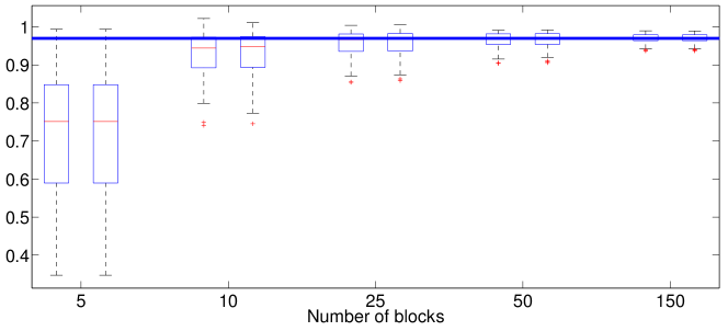
(a) $\tau_{n}\sim n$

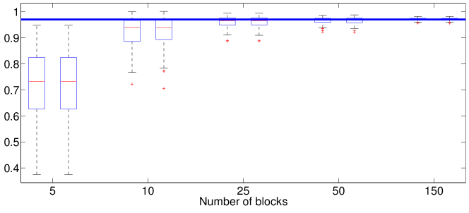
(b) $\tau_{n}\sim n^{1.5}$

Figure 1: Estimation of $\phi$ after $5,10,25,50$ and $150$ blocks, with two different initialization schemes: the stationary distribution (left) and the filtering distribution at the end of the previous block (right). The boxplots are computed with $100$ Monte Carlo runs.

The theoretical analysis of BOEM says that a sufficient condition for convergence is the increasing size of the blocks. On Figure 2, we compare different strategies for the definition of $\tau_{n}\stackrel{{\scriptstyle\mathrm{def}}}{{=}}T_{n}-T_{n-1}$. A slowly increasing sequence $\{\tau_{n}\}_{n\geq 0}$ is compared to different strategies using the same number of observations within each block. We consider the Linear Gaussian model:

$$X_{t+1}=\phi X_{t}+\sigma_{u}U_{t}\;,\qquad\qquad Y_{t}=X_{t}+\sigma_{v}V_{t}\;,$$

where $X_{0}\sim\mathcal{N}\left(0,\sigma_{u}^{2}(1-\phi^{2})^{-1}\right)$, $\{U_{t}\}_{t\geq 0},\{V_{t}\}_{t\geq 0}$ are i.i.d. standard Gaussian r.v., independent from $X_{0}$. Data are sampled using $\phi=0.9$, $\sigma_{u}^{2}=0.6$ and $\sigma_{v}^{2}=1$. All runs are started with $\phi=0.1$, $\sigma_{u}^{2}=1$ and $\sigma_{v}^{2}=2$. Figure 2 shows the estimation of $\phi$ over $100$ independent Monte Carlo runs (same conclusions could be drawn for $\sigma_{u}^{2}$ and $\sigma_{v}^{2}$). For each choice of $\{\tau_{n}\}_{n\geq 0}$, the median and first and last quartiles of the estimation are represented as a function of the number of observations.

We observe that BOEM does not converge when the block size sequence is constant and small: as shown in Figure 2, if the number of observations is too small ($\tau_{n}=25$), the algorithm is a poor approximation of the limiting EM recursion and does not converge. With greater block sizes ($\tau_{n}=100$ or $\tau_{n}=350$), the algorithm converges but the convergence is slower because it is initialized far from the true value and many observations are needed to get several estimations. BOEM with slowly increasing block sizes has a better behavior since many estimations are produced at the beginning and, once the estimates are closer to the true value, the bigger block sizes reduce the variance of the estimation.

Moreover, our convergence rates are given up to a multiplicative constant : the theory says that $\sum_{n}\tau_{n}^{-\gamma/2}<\infty$ where $\gamma$ is related to the ergodic behavior of the HMM (see assumptions HH5).

Even if the sequence is chosen to increase at a polynomial rate, we can have $\tau_{n}\sim c\ n^{\alpha}$ ($\alpha>1$) with a constant $c$ such that the first blocks are quite small to allow a sufficiently large number of updates of the parameters $\{\theta_{n},n\geq 1\}$. During a (deterministic) "burn-in" period, the first blocks can even be of a fixed length before beginning the “increasing” procedure.

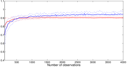
(a) $\tau_{n}=n^{1.1}$ (red) and $\tau_{n}=25$ (blue).

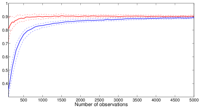
(b) $\tau_{n}=n^{1.1}$ (red) and $\tau_{n}=100$ (blue).

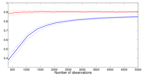
(c) $\tau_{n}=n^{1.1}$ (red) and $\tau_{n}=350$ (blue).

Figure 2: Estimation of $\phi$ with different block size schemes: the median (bold line) and the first and last quartiles (dotted line) are shown for $\tau_{n}=n^{1.1}$ (red), $\tau_{n}=100$ (black) and $\tau_{n}=350$ (purple). The quantities are computed with $100$ Monte Carlo runs.

4.2 Finite state-space HMM

Observations are sampled using $d=6$, $v=0.5$, $x_{i}=i\;,\forall i\in\{1,\dots,d\}$ and the true transition matrix is given by

$$m=\begin{pmatrix}0.5&0.05&0.1&0.15&0.15&0.05\\ 0.2&0.35&0.1&0.15&0.05&0.15\\ 0.1&0.1&0.6&0.05&0.05&0.1\\ 0.02&0.03&0.1&0.7&0.1&0.05\\ 0.1&0.05&0.13&0.02&0.6&0.1\\ 0.1&0.1&0.13&0.12&0.1&0.45\end{pmatrix}\;.$$

4.2.1 Comparison to an online EM based procedure

In this case, we want to estimate the states $\{x_{1},\dots,x_{d}\}$. All the runs are started from $v=2$ and from the initial states $\{-1;0;.5;2;3;4\}$. The experiment is the same as the one in [7, Section $3.2$]. The averaged BOEM is compared to an online EM procedure (see [2]) combined with Polyak-Ruppert averaging (see [9]). This online EM based algorithm follows a stochastic approximation update and depends on a step-size sequence $\{\gamma_{n}\}_{n\geq 0}$ which is chosen in the same way as in [7, Section $3.2$]. Figure 3 displays the empirical median and first and last quartiles for the estimation of $x_{2}$ with both averaged algorithms as a function of the number of observations. These estimates are obtained over $100$ independent Monte Carlo runs with $\tau_{n}=n^{1.1}$ and $\gamma_{n}=n^{-0.53}$. Both algorithms converge to the true value $x_{2}=2$ and these plots confirm the similar behavior of BOEM and the online EM of [2].

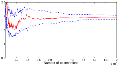
(a) Estimation of $x_{2}$ with averaged BOEM.

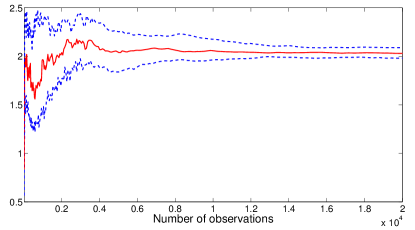
(b) Estimation of $x_{2}$ with averaged OEM.

Figure 3: Estimation of $x_{2}$ using the averaged online EM and averaged BOEM. Each plot displays the empirical median (bold line) and the first and last quartiles (dotted lines) over $100$ independent Monte Carlo runs with $\tau_{n}=n^{1.1}$ and $\gamma_{n}=n^{-0.53}$. The first ten observations are omitted for a better visibility.

4.2.2 Comparison to a recursive maximum likelihood procedure

In the numerical applications below, we give supplementary graphs to compare the convergence of the averaged BOEM with the convergence of the Polyak-Ruppert averaged RML procedure. The experiment is the same as the one in [7, Section $3.2$]. Figure 4 and 5 displays the empirical median and first and last quartiles of the estimation of $v$ and $m(1,2)$ over $100$ independent Monte Carlo runs. Both algorithms have a similar behavior for the estimation of these parameters.

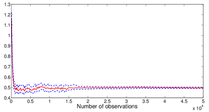
(a) Averaged BOEM.

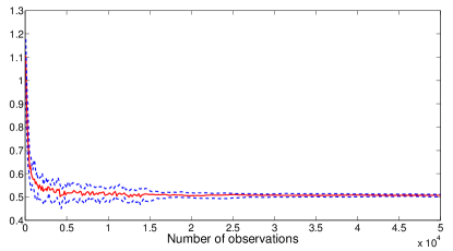
(b) Averaged RML.

Figure 4: Empirical median (bold line) and first and last quartiles (dotted line) for the estimation of $v$ using the averaged RML algorithm (right) and the averaged BOEM algorithm (left). The true values is $v=0.5$ and the averaging procedure is starter after $10000$ observations. The first $10000$ observations are not displayed for a better clarity.

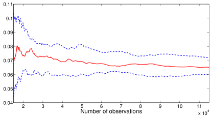
(a) Averaged BOEM.

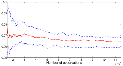
(b) Averaged RML.

Figure 5: Empirical median (bold line) and first and last quartiles (dotted line) for the estimation of $m(1,2)$ using the averaged RML algorithm (right) and the averaged BOEM algorithm (left). The true values is $m(1,2)=0.05$ and the averaging procedure is starter after $10000$ observations. The first $10000$ observations are not displayed for a better clarity.

4.3 Stochastic volatility model

Consider the following stochastic volatility model:

$$X_{t+1}=\phi X_{t}+\sigma U_{t}\;,\qquad\qquad Y_{t}=\beta\mathrm{e}^{\frac{X_{t}}{2}}V_{t}\;,$$

where $X_{0}\sim\mathcal{N}\left(0,(1-\phi^{2})^{-1}\sigma^{2}\right)$ and $(U_{t})_{t\geq 0}$ and $(V_{t})_{t\geq 0}$ are two sequences of i.i.d. standard Gaussian r.v., independent from $X_{0}$. Data are sampled using $\phi=0.8$, $\sigma^{2}=0.2$ and $\beta^{2}=1$. All runs are started with $\phi=0.1$, $\sigma^{2}=0.6$ and $\beta^{2}=2$.

In this model, the smoothed sufficient statistics $\{\bar{S}_{\tau_{n}}^{\chi,T_{n-1}}(\theta_{n-1},\mathbf{Y})\}_{n\geq 1}$ can not be computed explicitly. We thus propose to replace the exact computation by a Monte Carlo approximation based on particle filtering. The performance of the Stochastic BOEM is compared to the online EM algorithm given in [2] (see also [5]). To our best knowledge, there do not exist results on the asymptotic behavior of the algorithms by [2, 5]; these algorithms rely on many approximations that make the proof quite difficult (some insights on the asymptotic behavior are given in [2]). Despite there are no results in the literature on the rate of convergence of the Online EM algorithm by [2] we choose the step size $\gamma_{n}$ in [2] and the block size $\tau_{n}$ s.t. $\gamma_{n}=n^{-0.6}$ and $\tau_{n}\propto n^{3/2}$ (see [7, Section $3.2$] for a discussion on this choice). $50$ particles are used for the approximation of the filtering distribution by Particle filtering. We report in Figure 6, the boxplots for the estimation of the three parameters $(\beta,\phi,\sigma^{2})$ for the Polyak-Ruppert [9] averaged Online EM and the averaged BOEM. Both average versions are started after $20000$ observations. Figure 6 displays the estimation of $\phi$, $\sigma^{2}$ and $\beta^{2}$. This figure shows that both algorithms have the same behavior. Similar conclusions are obtained by considering other true values for $\phi$ (such as $\phi=0.95$). Therefore, the intuition is that online EM and Stochastic BOEM have the same asymptotic behavior. The main advantage of the second approach is that it relies on approximations which can be controlled in such a way that we are able to show that the limiting points of the particle version of the Stochastic BOEM algorithms are the stationary points of the limiting normalized log-likelihood of the observations.

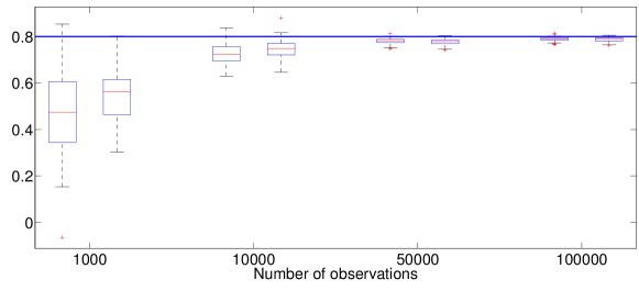
(a) Estimation of $\phi$.

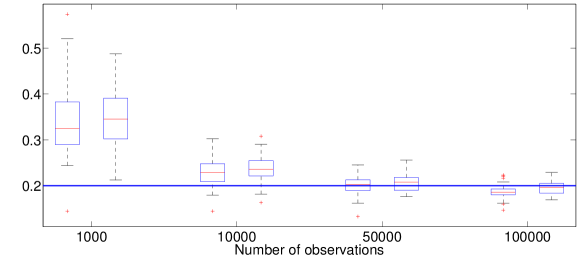
(b) Estimation of $\sigma^{2}$.

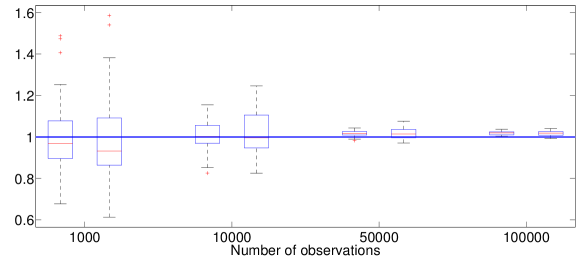
(c) Estimation of $\beta^{2}$.

Figure 6: Estimation of $\phi$, $\sigma^{2}$ and $\beta^{2}$ using the averaged online EM algorithm (left) and the averaged BOEM (right), after $n=\{1000,10k,50k,100k\}$ observations. The true value of $\phi$ is $0.8$.

We now compare the two algorithms when the true value of $\phi$ is (in absolute value) closer to $1$: we choose $\phi=0.95$, $\beta^{2}$ and $\sigma^{2}$ being the same as in the previous experiment.

As illustrated on Figure 7, the same conclusions are drawn for greater values of $\phi$.

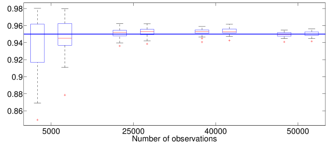
Figure 7: Estimation of $\phi$ using the averaged online EM algorithm (left) and the averaged BOEM algorithm (right), after $n=\{5k,25k,40k,50k\}$ observations. The true value of $\phi$ is $0.95$.

References

- [1] P. Billingsley. Probability and Measure. Wiley, New York, 3rd edition, 1995.
- [2] O. Cappé. Online EM algorithm for Hidden Markov Models. J. Comput. Graph. Statist., 20(3):728–749, 2011.
- [3] O. Cappé, E. Moulines, and T. Rydén. Inference in Hidden Markov Models. Springer, 2005.
- [4] J. Davidson. Stochastic Limit Theory: An Introduction for Econometricians. Oxford University Press, 1994.
- [5] M. Del Moral, A. Doucet, and S.S Singh. Forward smoothing using sequential Monte Carlo. arXiv:1012.5390v1, Dec 2010.
- [6] R. Douc, E. Moulines, and T. Rydén. Asymptotic properties of the maximum likelihood estimator in autoregressive models with Markov regime. Ann. Statist., 32(5):2254–2304, 2004.
- [7] S. Le Corff and G. Fort. Online Expectation Maximization based algorithms for inference in Hidden Markov Models. Technical report, arXiv:1108.3968, 2011.
- [8] G. Pólya and G. Szegő. Problems and Theorems in Analysis. Vol. II. Springer, 1976.
- [9] B. T. Polyak. A new method of stochastic approximation type. Autom. Remote Control, 51:98–107, 1990.