Automated analysis of quantitative image data using isomorphic functional mixed models, with application to proteomics data

Abstract

Image data are increasingly encountered and are of growing importance in many areas of science. Much of these data are quantitative image data, which are characterized by intensities that represent some measurement of interest in the scanned images. The data typically consist of multiple images on the same domain and the goal of the research is to combine the quantitative information across images to make inference about populations or interventions. In this paper we present a unified analysis framework for the analysis of quantitative image data using a Bayesian functional mixed model approach. This framework is flexible enough to handle complex, irregular images with many local features, and can model the simultaneous effects of multiple factors on the image intensities and account for the correlation between images induced by the design. We introduce a general isomorphic modeling approach to fitting the functional mixed model, of which the wavelet-based functional mixed model is one special case. With suitable modeling choices, this approach leads to efficient calculations and can result in flexible modeling and adaptive smoothing of the salient features in the data. The proposed method has the following advantages: it can be run automatically, it produces inferential plots indicating which regions of the image are associated with each factor, it simultaneously considers the practical and statistical significance of findings, and it controls the false discovery rate. Although the method we present is general and can be applied to quantitative image data from any application, in this paper we focus on image-based proteomic data. We apply our method to an animal study investigating the effects of cocaine addiction on the brain proteome. Our image-based functional mixed model approach finds results that are missed with conventional spot-based analysis approaches. In particular, we find that the significant regions of the image identified by the proposed method frequently correspond to subregions of visible spots that may represent post-translational modifications or co-migrating proteins that cannot be visually resolved from adjacent, more abundant proteins on the gel image. Thus, it is possible that this image-based approach may actually improve the realized resolution of the gel, revealing differentially expressed proteins that would not have even been detected as spots by modern spot-based analyses.

, , , and t1Supported by National Cancer Institute (CA-107304). t2Supported by National Institute for Alcohol Abuse (AA-016157). t3Supported by Statistical and Applied Mathematical Sciences Institute (SAMSI) Program on Analysis of Object Data (AOD).

1 Introduction

Image data are increasingly encountered in many areas of science and technology, including medicine, defense, robotics, security, and materials science. Image analysis involves the extraction of meaningful information from these data.

Some types of image analysis are performed subjectively by an expert user who is trained to visually extract the important features from the image. For example, a trained radiographer may inspect a CT scan to determine whether a patient has a tumor, or a trained pathologist may look at a scanned microscopic slide and determine the histology of a tumor. Other types of image information can be automatically extracted using a computer-based analysis of the digitized image based on an expert systems approach. For example, face recognition software can be used to identify an individual in an image, or optical character recognition software can be used to ascertain license plate numbers from still images taken at a toll booth. In these examples, the data are digitized and pattern recognition is used to perform discrimination, but the analysis is still qualitative in nature because the information of interest is the presence or absence of particular features in the image, not the magnitudes of the pixel intensities themselves.

In other image data, the magnitudes of the digitized pixel intensities actually represent an approximate quantification of some measurement of interest. For example, in functional magnetic resonance imaging (fMRI), magnetic images are obtained for serial slices of the brain, and the pixel intensities represent the amount of oxygenated blood flow to that part of the brain, which is a surrogate measure for the brain activity level. In 2D gel electrophoresis (2-DE)-based proteomics, the proteomic content of a biological sample is physically separated on a two-dimensional polyacrimidic gel by its isoelectric point (pH) and molecular mass. The gel is scanned to produce an image characterized by spots that correspond to proteins present in the sample. The intensities of the spots are rough measures of protein abundance. We refer to this type of image data as quantitative image data (QID), which is the primary focus of this paper.

A set of QID typically involves multiple scanned images from the same individual and/or from different individuals, with intensities observed over the same two-dimensional (or higher) domain. The overall goal of this type of quantitative image analysis (QIA) is to combine information across images to make statistical inferences about populations or about the effects of certain interventions on the populations represented in the images. One important specific goal of QIA is to identify which regions of the image differ significantly across treatment groups or populations. For example, in fMRI we might analyze images from individuals performing various functions in order to determine which parts of the brain are typically active during each activity, or we might wish to distinguish between different populations of patients with respect to their brain activity during a given activity, for example, in response to visual stimulus for children with and without attention deficit disorder. In proteomics, we aim to find which regions of the gel, and thus which proteins, are differentially expressed between cases and controls in a case-control study.

These image data sets are enormous in size and complex in nature, presenting numerous challenges in terms of storing, managing, analyzing and viewing the data. It is not uncommon to have hundreds or thousands of images in a given data set, with each image sampled on a grid of tens of thousands to millions of pixels. Managing and viewing data sets of this size is difficult; performing rigorous statistical analyses on the data is particularly challenging. Before statistical analysis can be performed, the raw, digitized images must undergo a number of processing steps, including alignment, background correction, normalization, denoising and artifact removal. These steps may involve technology-specific methods, and must be done before any further analysis takes place. We will not discuss preprocessing methods in detail in this paper, but will assume the researchers have applied suitable processing methods to the data before using the QIA methods we describe.

Feature extraction vs. image-based modeling: Researchers frequently use a feature extraction approach to analyze QID. They are motivated by the premise that the relevant information in the images is contained in well defined, discrete features that can be extracted by computing numerical summaries according to their estimated feature structure. The steps of a feature extraction approach are to identify the salient features in the images, quantify each feature for each individual, and then use standard univariate and multivariate statistical methods to determine which features are associated with the factors of interest. For example, in fMRI, the preprocessed pixel intensities can be integrated within predefined Regions of Interest (ROI), for example, brain regions, and then these regions can be analyzed to determine which regions are related to the underlying activity or population. In 2-DE proteomics, a spot-detection algorithm estimates distinct protein spots in the images. The protein spots are quantified and then surveyed to determine which are differentially expressed. This approach is computationally efficient because it reduces the data from complex, high-dimensional images to a vector of spot intensities, and can retain the relevant information contained in the QID, provided that all the salient features are properly detected and quantified.

The problem with this approach is that any information in the image not contained in one of the feature summaries will be completely lost to the analysis. In fMRI, there may be important differences within subregions of the predefined regions of interest that could be missed by integrating the entire region. In 2-DE, spot detection methods are not perfect and may fail to detect some differentially expressed proteins as distinct spots. One of the inherent dangers of this problem is that the researchers may never be aware that they missed anything—that there was information of significance in their data that was missed because of inadequate feature extraction.

An alternative to feature extraction is to model the images in their entirety using a suitable statistical modeling framework, which is a challenging endeavor we call an image-based modeling approach. To be appropriate for image-based modeling, an analytic method must possess the following three major characteristics: (1) sufficient flexiblity and adaptability to accommodate the local features that tend to characterize these complex, irregular data; (2) the ability to appropriately borrow strength spatially across the image; and (3) enough computational efficiency to be feasibly applied to data sets of this magnitude. Some examples of recently published image-based modeling methods include those of Reiss and Ogden (2009), who constructed a generalized linear model method for image predictors, and Smith and Fahrmeir (2007), who analyzed fMRI data using Bayesian variable selection on image pixels and an Ising prior to model spatial correlation among the variable selection parameters. QID can be viewed as functional data with the two-dimensional domain given by the rows and columns of the image and the range given by the pixel intensities, and thus can be analyzed using a functional data analysis [FDA, Ramsay and Silverman (1997)] approach.

Recent work on Functional Mixed Models (FMM) [Guo (2002), Morris et al. (2003), Morris and Carroll (2006), Morris et al. (2006), Morris et al. (2008)] provides a general modeling framework useful for modeling many types of functional data, but has not yet been adapted for use with image data. In this paper we present a unified, Bayesian image-based analysis approach for QID based on a version of the FMM suitable for higher dimensional image data. The model fitting is done using an isomorphic transformation approach, which we define and introduce in Section 3.2. The method can simultaneously model the effects of multiple factors on the images through fixed effects and can account for correlations between images that are induced by the design through random effect modeling. The isomorphic modeling approach results in efficient calculations and, with suitable transformation, can accommodate nonstationary features in the covariance matrices, and result in adaptive smoothing and borrowing of strength across pixels in each dimension while the inference is performed. The method yields posterior probabilities of specified effect sizes that can be interpreted as local false discovery rates [FDR, Benjamini and Hochberg (1995), Storey (2003)]. The posterior probabilities can be used in Bayesian inference to flag regions of the curves as significant while considering both practical and statistical significance and controlling the FDR. The software to implement this method can be run automatically with little user input, and is efficient enough to handle even very large image data sets. Although this method is generally applicable to all QID, in this paper we focus on 2-DE data. We show that this adaptive, image-based approach can find results that would have been missed with standard spot-level analyses, and may extract more protein information from the gels than was previously known to be present.

In Section 2 we discuss image-based proteomics and standard analysis approaches, and introduce the brain proteomics data set that we consider in this paper. In Section 3 we describe the methodology: we overview functional mixed models, describe our general isomorphic approach to model fitting, and present the isomorphic functional mixed model for higher dimensional image data. Also, we describe how to conduct Bayesian FDR-based inference using the output data and present an image compression approach that can be used optionally to speed up calculations. In Section 4 we apply this method to the brain proteomics data set and compare and contrast results with a feature extraction approach. We finish with a discussion of the implications of our results for 2-DE proteomics and as a general methodology for quantitative image data analysis in Section 5.

2 Image-based proteomics data

2.1 Introduction to proteomics

Over the past two decades, advances in genomics have fueled increased interest in the field of proteomics. Proteomics differs from genomics in that the former field involves the direct measurement of proteins rather than their precursors, genes and messenger RNA. Our focus is on the use of proteomics for biomarker discovery, which involves the measurement of the relative abundance of proteins across different samples to determine which are differentially expressed across groups or correlated to a factor of interest. The proteins of interest can then be validated and further studied for possible clinical applications, for example, for early detection of cancer or as markers of response to a particular cancer therapy. Various types of proteomics data can be considered quantitative image data, including liquid chromatography–mass spectrometry (LC–MS) and 2D gel electrophoresis (2-DE).

While LC–MS is growing in importance, the major workhorse in biomarker discovery proteomics to date has been 2-DE. The process of 2-DE involves staining and denaturing the biological sample, running it through a polyacrimidic gel, and separating the proteomic content of the sample by isolectric point (pH) and then by molecular mass. The gel is then digitally scanned to produce an image of the stained spots that correspond to proteins present in the sample, which are double indexed by their molecular mass and pH. The spots on the gel physically contain the actual proteins, so protein identification is easily accomplished by cutting out the spot, enzymatically digesting it, and using MS–MS to ascertain its identity. One variant of 2-DE that may yield more accurate relative quantifications is 2D difference gel electrophoresis [DIGE, Lilley (2003), Karp and Lilley (2005)], which involves differentially labeling two samples with two different dyes, loading them onto the same gel, and then scanning the gel with two different lasers, each of which specifically picks up one of the two dyes. When comparing two groups, paired samples from each group can be run on the same gel, effectively conditioning the gel effect out of the analysis. In more general problems, one dye (the active channel) can be used for the primary sample and the other dye (the reference channel) used on some common reference material used on all gels so that it may serve as an internal normalization factor.

2-DE has been criticized for various perceived limitations of the technology, including its limited ability to measure proteins with medium or low abundance or to resolve co-migrating proteins with similar pH/mass combinations [Gygi et al. (2000)]. Although the technology itself may possess some technical limitations, a major factor limiting the realized potential of 2-DE is a lack of efficient and effective algorithms to process and analyze the gel images. More effective analytic methods that better extract proteomic information from the gel images may help the technology more fully realize its potential.

2.2 Spot-based analysis of 2-DE proteomic data

Nearly all existing 2-DE gels are analyzed using a feature extraction approach whereby spots are detected and quantified for different gel images and then analyzed to ascertain which are differentially expressed. The success of a feature extraction approach depends on the effectiveness of the feature detection and quantification method used and, until recently, the predominant approaches used for spot detection and quantification had major problems. Traditional approaches based on spot detection on individual gels followed by matching spots across gels suffer from problems with missing data, spot detection errors, spot matching errors and spot boundary estimation errors [Clark and Gutstein (2008), Morris, Clark and Gutstein (2008)]. The abundance of these errors may be partially responsible for some researchers concluding the technology is ineffective. In recent years, alternative spot detection strategies have been developed that mitigate these errors to a degree, and include Pinnacle, a method we have developed [Morris, Clark and Gutstein (2008), Morris et al. (2010)], and commercial packages SameSpots by Nonlinear Dynamics (Newcastle upon Tyne, UK), Redfin Solo by Ludesi (Malmo, Sweden) and Delta2D by Decodon (Greifswald, Germany). While improving from past methods, these spot-based approaches are still far from perfect, and, in particular, still have some difficulty resolving distinct co-migrating proteins that are present in the same spot. Thus, there may be more to gain by using an image-based modeling approach.

2.3 Image-based analysis approaches for 2-DE

Spot-based approaches are almost universally used for the analysis of 2-DE data. We know of only one paper in the current literature that describes the application of an image-based modeling approach. Faergestad et al. (2007) presented a pixel-based method for pairwise analysis of 2-DE data that involves the application of partial least squares regression (PLSR) to the vectorized gel images (after preprocessing). Faergested et al. used a jacknife procedure to conduct inference, repeatedly applying the PLSR to each leave-one-out cross-validation sample and then performing a $t$-test at each pixel using the cross-validation regression coefficients as the data. In order to avoid flagging pixels that were statistically but not practically significant, they restricted their attention to pixels with a certain minimum standard deviation across samples. The general image-based method we introduce in this paper is not limited to pairwise inference; it can account for correlation among images from the same subject or batch; it performs adaptive smoothing as part of the estimation and inference; and it yields rigorous unified FDR-based Bayesian inference that simultaneously accounts for both statistical and practical significance. Our method can be applied to any type of image-based proteomics data, including LC–MS, 2-DE and DIGE.

2.4 Motivating example: Cocaine addiction brain proteomics study

The methods we develop in this paper are applied to proteomic data from a neurobiology study on cocaine addiction. The study aimed to identified neurochemical changes in the brain that are associated with the transition from nondependent drug use to addiction. The addiction process is conceptualized as an increasing motivation to seek drugs, resulting in increased drug intake, loss of control over drug intake and compulsive drug taking. Previous studies suggest that prolonged exposure to cocaine or opiate drugs leads to increased self-administration and a pronounced elevation in reward thresholds [Leith and Barrett (1976), Kokkinidis, Zacharko and Predy (1980), Markou and Koob (1992), Schulteis et al. (1994)]. Neurochemical changes in parts of the basal forebrain structure, the extended amygdala, parallel these decreases in the function of the reward system [Parsons, Koob and Weiss (1995), Weiss et al. (1992), Heinrichs et al. (1995), Richter and Weiss (1999)]. These data suggest that substance dependence or addiction produces a pronounced dysregulation of the brain’s reward systems, and that neurochemical changes in the extended amygdala may provide a substrate for such dysfunction. The neurochemical changes may involve cellular effects at the translational and post-translational levels that alter protein expression and function, and thus may be detected by proteomic analysis.

An animal study to investigate these concepts used a model developed by Ahmed and Koob (1998). The animal model was based on rats that were trained to obtain cocaine by pressing a lever. Six rats were given short durations of drug access (1 hour/day), and 7 rats were given long durations of drug access (12 hours/day). The study included 8 control rats. The rats were eventually euthanized, and their brain tissue was harvested and microdissected to extract various regions of the extended amygdala. Tissues from the brain samples were then subjected to 2-DE to assess their proteomic content. The goal was to compare and contrast protein expression and modification associated with excessive levels of cocaine intake and to compare tissues from animals given long versus short access to the drug. The data we analyzed for this paper were obtained from the the central nucleus region of the extended amygdala. The data set contains a total of 53 gels from 21 rats, with roughly 2–3 gels per rat.

3 Methods

In this section we review previous work on functional mixed models and wavelet space modeling for 1D functional data, and then discuss how this approach can be used with other transformations, that is, not just wavelets. Thereafter, we describe how to adapt this method to model image data and discuss how to perform rigorous FDR-based Bayesian inference from its output.

3.1 Functional mixed models and wavelet-based modeling

For back-ground, here we describe the wavelet-based functional mixed models method (WFMM) of Morris and Carroll (2006). Suppose we observe a sample of $N$ curves $Y_{i}(t),i=1,\ldots,N$, each defined on a compact set ${\mathcal{T}}$. The FMM is given by

$$\mathbf{Y}(t)=X\mathbf{B}(t)+Z\mathbf{U}(t)+\mathbf{E}(t),$$ (1)

where $\mathbf{Y}(t)=\{Y_{1}(t),\ldots,Y_{N}(t)\}^{\prime}$ is a vector of observed functions, “stacked” as rows. Here, $\mathbf{B}(t)=\{B_{1}(t),\ldots,B_{p}(t)\}^{\prime}$ is a vector of fixed effect functions with corresponding $N\times p$ design matrix $X$, $\mathbf{U}(t)=\{U_{1}(t),\ldots,U_{m}(t)\}^{\prime}$ is a vector of random effect functions with corresponding $N\times m$ design matrix $Z$, and $\mathbf{E}(t)=\{E_{1}(t),\ldots,E_{N}(t)\}^{\prime}$ is a vector of functions representing the residual error processes. The effect functions measure the partial effect of the corresponding covariate at position $t$ of the functions. The set of random effect functions $\mathbf{U}(t)$ is a realization from a (mean zero) multivariate Gaussian process with $m\times m$ between-function covariance matrix $P$ and within-function covariance surface $Q(t_{1},t_{2})$, denoted by $\mathbf{U}(t)\sim{\mathcal{MGP}}(P,Q)$ and implying that $\operatorname{cov}\{U_{b}(t_{1}),U_{b^{\prime}}(t_{2})\}=P_{bb^{\prime}}Q(t_{1},t_{2})$. The residual errors are assumed to follow $\mathbf{E}(t)\sim{\mathcal{MGP}}(R,S)$, independent of $\mathbf{U}(t)$. The random effect or residual error portions of the model can be stratified to allow covariances indexed by some factor, $Z\mathbf{U}(t)=\sum_{h=1}^{H}Z_{h}\mathbf{U}_{h}(t)$ with $\mathbf{U}_{h}(t)\sim{\mathcal{MGP}}(P_{h},Q_{h})$ or $\mathbf{E}(t)=\sum_{c=1}^{C}\mathbf{V}_{c}\mathbf{E}_{c}(t)$ with $\mathbf{V}_{c}$ a vector whose $i$th element is 1 if curve $i$ is from stratum $c$ and $\mathbf{E}_{c}\sim{\mathcal{MGP}}(R_{c},S_{c})$.

In practice, observed functional data are sampled on some discrete grid. Assuming all observed functions are sampled on the same fine grid $\mathbf{t}=(t_{1},\ldots,t_{T})$, the discrete version of (1) is

$$Y=XB+ZU+E,$$ (2)

where $Y$ is an $N\times T$ matrix of observed curves on the grid $\mathbf{t}$, $B$ is a $p\times T$ matrix of fixed effects, $U$ is an $m\times T$ matrix of random effects, and $E$ is an $N\times T$ matrix of residual errors. Following Dawid (1981), $U$ follows a matrix normal distribution with $m\times m$ between-row covariance matrix $P$ and $T\times T$ between-column covariance matrix $Q$, which we denote by $U\sim{\mathcal{MN}}(P,Q)$, implying $\operatorname{cov}(U_{ij},U_{i^{\prime}j^{\prime}})=P_{ii^{\prime}}Q_{jj^{\prime}}$. The residual error matrix $E$ is assumed to be ${\mathcal{MN}}(R,S)$. The within-random effect curve covariance surface $Q$ and residual error covariance surface $S$ are $T\times T$ covariance matrices that are discrete approximations of the corresponding covariance surfaces in ${\mathcal{T}}\times{\mathcal{T}}$.

Morris and Carroll (2006) used a wavelet basis modeling approach to fit the model (2), which involves three steps. First, a fast algorithm called the discrete wavelet transform [$\operatorname{DWT}$, Mallat (1989)] is applied to each of the $N$ observed functions on grid $\mathbf{t}$ to yield a vector of $T$ wavelet coefficients for each function, effectively rotating the data axes to transform the data into the wavelet space. Second, a Markov chain Monte Carlo (MCMC) procedure is used to obtain posterior samples from a wavelet-space version of model (2). The wavelet-space covariance matrices for the random effect functions and residual errors are modeled as diagonal, but with different variances for each wavelet coefficient, and spike-slab priors are assumed on the fixed effects’ wavelet coefficients. These assumptions are parsimonious, yet accommodate nonstationary features in the data-space covariance matrices $Q$ and $S$ and induce adaptive regularization of the fixed and random effect functions, $B_{a}(t)$ and $U_{b}(t)$ [Morris and Carroll (2006)]. Third, the inverse $\operatorname{DWT}$ is applied to the the posterior samples of the wavelet-space parameters to yield posterior samples of the parameters in the data-space model (2), which can be used to perform Bayesian inference.

3.2 Isomorphic modeling of functional mixed models (ISO-FMM)

The WFMM is just one example of a general approach to fitting functional mixed models we call an isomorphic approach (ISO-FMM), which we introduce here. The same basic three-step approach underlying the WFMM can be applied using isomorphic transformations not involving wavelets if desired. We define an isomorphic transformation as one that preserves all of the information in the original data, that is, is invertible. More precisely, given row vector $\bf y\in\Re(T)$, we say a transform $f\dvtx\Re(T)\rightarrow\Re(T)$ is isomorphic if there exists a reverse transform $f^{-1}$ such that $f^{-1}\{f(\bf y)\}=\mbox{\bf y}$. The wavelet transform is isomorphic because $\operatorname{IDWT}(\operatorname{DWT}(\bf y))=\bf y$, but isomorphic transformations can be constructed in other ways as well, for example, by using other basis functions including Fourier bases, spline bases and certain empirically determined basis functions like functional principal components.

Suppose we observe $N$ functions all on the same fine grid $\mathbf{t}$ of length $T$, resulting in $N\times T$ data matrix $Y$ whose rows are the observed functions and columns index the grid locations. The following steps describe the general steps of a Bayesian implementation of the ISO-FMM for functional data:

1. Transform each of the rows of $Y$ using an isomorphic transformation $f$, represented as $D=f(Y)$, with $f(\cdot)$ applied to a matrix implying here the transform $f$ is applied separately to each row. Rather than indexing positions within the curve, the columns of $D$ will index items in the transformed space, for example, basis coefficients. We can think of the induced functional mixed model in the transformed space with the columns of $D,B^{*}=f(B),U^{*}=f(U)$, and $E^{*}=f(E)$ indexing coefficients in the alternative space. We refer to this as the transformed-space FMM.

2. Apply an MCMC procedure to the transformed-space FMM to obtain posterior samples of all of its parameters. This requires specification of (a) parsimonious assumptions on the covariance matrices $Q^{*}$ and $S^{*}$ that are sufficiently flexible to capture important features of $Q$ and $S$, and (b) a prior distribution on the fixed effects in the transformed-space FMM to induce effective regularization of the fixed effect functions $B^{*}$.

3. Apply the inverse isomorphic transform $f^{-1}$ to the posterior samples of the functional quantities in the transformed-space FMM to obtain posterior samples from the original data-space FMM (2), where Bayesian inference is performed.

This approach could also be applied in a frequentist context. That would involve fitting the transformed-space model with some explicit roughness penalties in appropriate places, for example, the fixed and random effect functions, to induce adaptive smoothing, and then transforming the estimated quantities back to the data space. This would easily yield estimates, but more work would need to be done to obtain inferential quantities.

The use of an isomorphic transformation ensures that the representation in the transformed data retains all of the information contained in the original data, that is, is “lossless,” and thus any basis coefficients can be considered as transformed raw data rather than estimated parameters. Thus, the transformed-space model is isomorphic to the data-space model. This allows us to perform the modeling in the transformed space, where it may be possible to perform modeling and regularization more parsimoniously and conveniently, and yet obtain valid inference in the data-space model, where the parameters are more clearly interpretable.

For many isomorphic transformations, it is possible to assume parsimonious structures for $Q^{*}$ and $S^{*}$ in the basis space and still accommodate a rich class of structures for data space within curve covariance matrices $Q$ and $S$. For example, using a Fourier transform, any stationary covariance matrix can be represented by uncorrelated Fourier coefficients, so diagonal $Q^{*}$ and $S^{*}$ are fully justified if we are willing to assume stationarity in $Q$ and $S$. Diagonal assumptions on $Q^{*}$ and $S^{*}$ allow the transformed-space FMM to be fit one column at a time, making the procedure highly parallelizable and reducing the memory requirements of the software. This assumption may also be justifiable in some empirically-determined basis spaces such as FPC. For wavelets, the whitening property of the transform makes diagonal $Q^{*}$ and $S^{*}$ a reasonable working assumption that accommodates many commonly encountered nonstationary features. For a given isomorphic transformation, one must decide what parsimonious assumptions are reasonable in the basis space, and carefully consider what constraints these assumptions induce in the data space.

Another advantage of transformed-space modeling is that for many isomorphic transforms, there are natural prior distributions on basis space coefficients that can induce regularization of the functional effects in the model and effectively act like roughness penalties. For example, with wavelets, a sparsity prior that has a spike at zero and medium-to-heavy tails like a spike-slab prior leads to adaptive regularization of the underlying effect function. Spline bases are frequently regularized by second-order penalties, which can be induced by a Gaussian prior. First-order penalties can be induced by double-exponential priors.

Although orthonormal linear isomorphic transformations are convenient to use because they represent a simple rotation of the axes, they are not the only possibility. The transform does not have to be orthonormal or even linear. With an orthonormal transform, i.i.d. white noise has the same distribution and total energy in both the data and basis space, but these are not necessary properties for the FMM. With linear transforms [$f(Y)=YW^{\prime}$ for some matrix $W^{\prime}$], a Gaussian model in the data space induces a Gaussian model in the transformed space, and vice-versa, but this is also not absolutely necessary for valid modeling. For example, one could specify a Gaussian model in the transformed space that is used for the fitting, and this would correspond to some non-Gaussian model in the data space that might not have a simple closed form, but which could still be a valid and reasonable data-space likelihood.

If the set of functions jointly have a very sparse representation in the chosen basis space, it may be possible and advantageous to use an approximately isomorphic transformation of lower dimension that still retains almost all of the information for the original functions. We describe a way to perform this compression in the multiple function context in Section 3.5.

Many methods in the existing statistical literature use a basis function approach to represent functions or vectors, but rather than transformed data the coefficients are typically treated as parameters to estimate and the transforms are not isomorphic but lower rank projections. There are some methods in the current statistical literature that effectively use an isomorphic modeling approach [e.g., wavelet regression, Clyde, Parmigiani and Vidakovic (1998); spectral analysis of stationary time series, Diggle and Al Wasel (1997); nonisotropic modeling of geostatistical data, Sampson and Guttorp (1992)]; however, to our knowledge, this has not been discussed previously as a general modeling strategy. Our intended contributions here are to (1) explicitly offer an isomorphic approach as a general modeling strategy and (2) apply this approach to functional mixed modeling.

3.3 ISO-FMM for quantitative image data

In this section we introduce a functional mixed model for image data, describe how to model image data using our isomorphic transformed-space approach, and provide implementation details using higher dimensional wavelet transforms. Even though these results hold generally for higher dimensional images, we present the results for 2D images for ease of exposition.

3.3.1 Functional mixed models for quantitative image data

Suppose we have a sample of $N$ images, $Y_{i},i=1,\ldots,N$, with each $Y_{i}$ a $T_{1}\times T_{2}$ matrix containing the image intensities sampled on a regular, equally-spaced two-dimensional grid $(\mathbf{t}_{1},\mathbf{t}_{2})$ with $\mathbf{t}_{1}=(t_{11},\ldots,t_{1T_{1}})^{\prime}$ and $\mathbf{t}_{1}=(t_{21},\ldots,t_{2T_{2}})^{\prime}$. A functional mixed model for these image data, with $(t_{1},t_{2})$ a coordinate on the grid, can be written as

$$Y_{i}(t_{1},t_{2})=\sum_{a=1}^{p}X_{ia}B_{a}(t_{1},t_{2})+\sum_{b=1}^{m}Z_{ib}U_{b}(t_{1},t_{2})+E_{i}(t_{1},t_{2}),$$ (3)

where $B_{a}$ and $U_{b}$ are fixed and random effect images, respectively, which measure the effects of scalar fixed or random effect covariates on the corresponding location of the image $Y$, and $E_{i}$ contains the residual error images. The $U_{b}$ and $E_{i}$ are mean zero Gaussian processes defined on the surface, with corresponding between-image covariance matrices $P$ and $R$, respectively, and four-dimensional within-image covariance surfaces $Q(t_{1},t_{2},t^{\prime}_{1},t^{\prime}_{2})$ and $S(t_{1},t_{2},t^{\prime}_{1},t^{\prime}_{2})$ summarizes the covariance between locations $(t_{1},t_{2})$ $(t^{\prime}_{1},t^{\prime}_{2})$ of the random effect and residual error images, respectively.

Let each image be represented by a row vector of length $T_{1}*T_{2}$, $\mathbf{y}_{i}=\{\operatorname{vec}(Y_{i})\}^{\prime}$, where $\operatorname{vec}$ is the column stacking vectorizing operator. If we let $Y$ be the $N\times T(=T_{1}*T_{2})$ matrix whose rows contain the vectorized images, then the discrete image mixed model can be written as

$$Y^{I}=XB^{I}+ZU^{I}+E^{I},$$ (4)

with each row of $B^{I}$ and $U^{I}$ containing one of the vectorized fixed or random effect images, respectively, that measure the effect of a scalar fixed or random effect covariate on the corresponding location of the image, and with the rows of $E^{I}$ containing the vectorized “residual error images.” The columns index the pixels in the image. The superscript “$I$” simply is a reminder that these quantities are based on images. As before, we assume that $U^{I}\sim{\mathcal{MN}}(P,Q)$ and $E^{I}\sim{\mathcal{MN}}(R,S)$, with $P$ and $R$ being $m\times m$ and $N\times N$ matrices defining covariances between images, and $Q$ and $S$ being $T\times T$ within-function two-dimensional covariance matrices for the random effects and residuals that model the covariance between different positions within the images. For example, $Q\{t_{1}+(t_{2}-1)*T_{1},t_{1}^{\dagger}+(t_{2}-1)^{\dagger}*T_{1}\}$ describes the covariance between $U^{I}_{b}(t_{1},t_{2})$ and $U^{I}_{b}(t_{1}^{\dagger},t_{2}^{\dagger})$. Note that any reasonable structure on these within-image covariance matrices should not just model the autocovariance based on the proximity within the vector $\mathbf{y}_{i}$, but rather the proximity within the higher dimensional image $Y_{i}^{I}$, that is, in all dimensions.

3.3.2 ISO-FMM for quantitative image data

The ISO-FMM approach for 1D functions described in Section 3.2 can be applied to QID, as well, using isomorphic transforms and inverse transforms that operate on the higher dimensional functions, for example, images. The covariance assumptions in the transformed space and the regularization prior distributions should be chosen to induce appropriate spatial correlation, adaptive smoothing and borrowing of strength in all dimensions.

The isomorphic transform $f$ in the image space will map the $T=T_{1}\times T_{2}$ pixels to a set of alternative transformed-space coefficients, $D^{I}_{i}=f(Y^{I}_{i})$. This transform can be constructed a number of different ways. One natural way is to take tensor products of suitable 1D transforms, leading to a separable transform. It is also possible to use special bases constructed for image data. Depending on the resolution of the images and transform used, computational feasibility can become an issue because the transform will have to be applied to all $N$ observed images as well as to all $p$ fixed effect images for each of $M$ posterior samples. After transformation, a model is then proposed in the transformed space.

If the transform is linear, then the Gaussian assumptions from (4) hold in both the data and transformed space, and our transformed-space model is given by

$$D^{I}=XB^{I*}+ZU^{I*}+E^{I*},$$ (5)

with the rows of $D^{I},B^{I*}=f(B^{I}),U^{I*}=f(U^{I}),$ and $E^{I*}=f(E^{I})$ containing the transformed representations for each of the corresponding image-based quantities in (4), with $U^{I*}\sim MN(P,Q^{*})$ and $E^{I*}\sim MN(R,S^{*})$. As before, $f(A)$ for some matrix $A$ means applying the transformation $f$ sequentially on the rows of $A$. If a separable linear transform is used, then the linear transform matrix for the vectorized images can be explicitly defined as follows. Suppose we obtain a matrix of coefficients $D^{I}_{i}$ from the sampled image $Y^{I}_{i}$ by applying a linear transform $W_{1}$ to the rows of the image and $W_{2}$ to the columns, that is, $D^{I}_{i}=W_{1}Y^{I}_{i}W_{2}^{\prime}$. This transformation can be explicitly represented as $\mathbf{d}_{i}=\mathbf{y}_{i}{\mathcal{W}}^{\prime}$, where $\mathbf{y}_{i}=\operatorname{vec}(Y^{I}_{i})^{\prime}$ and $\mathbf{d}_{i}=\operatorname{vec}(D^{I}_{i})$ are the vectorized image and coefficient matrix, respectively, ${\mathcal{W}}^{\prime}=(W_{2}\otimes W_{1})$ is the linear transformation matrix, and $\otimes$ is the Kronecker product. This representation makes it easy to explicitly see the connections between the data-space and transformed-space matrix models (4) and (5) for the QID context as $D^{I}=Y^{I}{\mathcal{W}}^{\prime}$, $B^{I*}=B^{I}{\mathcal{W}}^{\prime}$, $U^{I*}=U^{I}{\mathcal{W}}^{\prime}$, and $E^{I*}=E^{I}{\mathcal{W}}^{\prime}$, and $Q^{*}={\mathcal{W}}^{\prime}Q{\mathcal{W}}$ and $S^{*}={\mathcal{W}}^{\prime}S{\mathcal{W}}$. If $W_{1}$ and $W_{2}$ are orthogonal, then it follows that ${\mathcal{W}}$ is also orthogonal. These results generalize to general $r$-dimensional functions stacked as vectors using ${\mathcal{W}}^{\prime}=(W_{r}\otimes W_{r-1}\otimes\cdots\otimes W_{1})$.

3.3.3 Implementation details using wavelets

The same properties that make wavelet bases convenient for isomorphic modeling in 1D functional data (fast calculations, compact support, whitening property, joint frequency–time representation, sparse representations for broad classes of data) also make them useful for modeling QID. Here, we will describe the implementation details for ISO-FMM using higher dimensional wavelet transforms to construct the isomorphic transformations, which involves three factors: choice of transform, specification of covariance structure, and regularization prior.

There are various ways to construct isomorphic transforms for image data using wavelet bases. These transforms can be separable or nonseparable. A separable, or rectangular, transform is easily constructed by applying the 1D $\operatorname{DWT}$ separately to each row and each column of the image. As mentioned in Section 3.1, after applying the wavelet transform to a vector of data, the resulting wavelet coefficients are double-indexed by scale $j=1,\ldots,J$ and location $k=1,\ldots,K_{j}$. If we apply a separable 2D wavelet transform, each coefficient is quad-indexed by row scale $j_{1}$ and location $k_{1}$, and column scale $j_{2}$ and location $k_{2}$.

Nonseparable transforms can also be used. Although they are not represented as simple tensor products of 1D transforms, they are constructed using linear operators, and so still represent a linear transformation. The most commonly used nonseparable wavelet transform is a square transform. This type of decomposition yields three types of wavelet coefficients at each scale $j=1,\ldots,J$, corresponding to horizontal, vertical and diagonally-oriented wavelet bases. In this case, the wavelet coefficients are triple-indexed by scale ($j=1,\ldots,J$), orientation {$l=1$ (row details), 2 (column details), 3 (2D details)} and location ($k=1,\ldots,K_{jl}$). The square wavelet transform tends to better model local behavior and leads to more parsimonious representations than the rectangular transform, and so is commonly used in practice. With the basis functions aligned with the principal axes (horizontal, vertical and diagonal), a disadvantage of the square transform is that sometimes it does not efficiently represent smoother contours or features of the images that do not align with the principal axes [Do and Vetterli (2001)]. This leads to less effective adaptive smoothing for images with these types of features. Other 2D wavelet transforms have been constructed for this purpose and could be used in place of the square transform, for example, curvelets [Candes and Donoho (2000)], contourlets [Do and Vetterli (2005)] or qincunx wavelets [Feilner, Van De Ville and Unser (2005)]. We choose to use the square nonseparable wavelet transform for 2-DE data because the key features of the images, the spots, are aligned with the horizontal and vertical axes and so should be well represented by them. We found them to be more efficient than the rectangular separable transform which contains many long, thin basis functions constructed by combining a low frequency basis in one dimension (small $j$) and high frequency basis in the other (large $j$).

Again, motivated by the whitening property of the wavelet transform, we model the wavelet coefficients as independent, that is, $Q^{*}=\operatorname{diag}(q_{jlk})$ and $S^{*}=\operatorname{diag}(s_{jlk})$, allowing each coefficient triple-indexed by its scale $j$, orientation $l$ and location $k$ to have its own variance component. The independence leads to parsimonious modeling, while the heteroscedasticity accommodates nonstationary spatial features in the data space matrices $Q$ and $S$. In Supplementary Material, we illustrate through plots and movies [Morris (2010)] the effective spatial covariance structures of $Q$ and $S$ induced by independent heteroscedastic wavelet space models for our 2-DE data. It accommodates spatial covariance in all directions, based on proximity horizontally, vertically and diagonally, and the strength of this spatial covariance is allowed to vary across different parts of the image. This adaptive handling of spatial correlation is important in 2-DE, since we expect strong autocorrelation within spots that rapidly falls off outside of the spot, and we expect a more slowly decaying autocorrelation in nonspot background regions of the gel. Further, the structure allows different image-to-image variances for different pixels in the image, which is important to obtain accurate pixelwise inference, since we expect different protein spots to have different variances. These principles generalize to higher dimensional images when the corresponding higher dimensional $\operatorname{DWT}$ is used for transformation.

We assume the spike-Gaussian slab prior on the wavelet coefficients for the fixed effects, which is written as

$$B^{*}_{ajlk} = \gamma^{*}_{ajlk}{\mathcal{N}}(0,\tau_{ajl})+(1-\gamma^{*}_{ajlk})I_{0},$$

$$\gamma^{*}_{ajlk} = \operatorname{Bernoulli}(\pi_{ajl}),$$

with regularization parameters $\pi$ and $\tau$ indexed by covariate $a$, scale $j$ and orientation $l$, and estimated from the data using the empirical Bayes procedure similar to Morris and Carroll (2006), as detailed in a supplementary article [Morris (2010)]. This induces adaptive smoothing of the fixed effect images $B_{a}(t_{1},t_{2})$. By indexing the parameters by covariate, we allow for different regularization parameters for different fixed effect images, and by indexing by scale $j$ and orientation $l$, we are able to naturally accommodate different degrees of smoothness horizontally, vertically and diagonally within the fixed effect images.

After specifying vague proper priors on the variance components, we are left with a fully specified Bayesian model for the transformed-space FMM (2). We use a Markov chain Monte Carlo (MCMC) procedure to obtain posterior samples of the transformed-space fixed effect functions $B^{*}$, and then apply the inverse 2D wavelet transform to them to obtain posterior samples of the data-space fixed effect functions $B$, which are used for Bayesian inference. The MCMC details are presented in the supplementary article by Morris (2010).

3.4 Bayesian FDR-based inference

Given the posterior samples of$B_{a}(t_{1},t_{2})$, the fixed effect image describing the effect of covariate $X_{a}$ on the images as a function of position $(t_{1},t_{2})$, we can perform Bayesian inference to flag significant regions of the curves by extending the approach used in Morris et al. (2008), as follows.

First, we must define the effect size that is of practical significance, say, $\delta$. For example, if the image intensities are modeled on a $\log_{2}$ scale, then $\delta=1$ would correspond to a two-fold difference. From the posterior samples of $B$, we can compute the posterior probability of an effect size of at least $\delta$, $p_{a}^{\delta}(t_{1},t_{2})=\operatorname{Prob}\{|B_{a}(t_{1},t_{2})|>\delta\}$, which can be plotted in what we call a probability discovery image, and define significant regions of the image as those with $p^{\delta}_{a}(t_{1},t_{2})>\phi$ for some threshold $\phi$. The quantities $1-p^{\delta}_{a}(t_{1},t_{2})$ can be considered $q$-values, or estimates of the local false discovery rate [Storey (2003)], as they measure the probability of a false positive if position $(t_{1},t_{2})$ is called a “discovery,” defined as a region in the image with at least $\delta$ effect size.

The significance threshold $\phi$ can be determined using classical Bayesian utility considerations such as those of Mueller et al. (2004) based on the elicited relative costs of false positive and false negative errors. Alternatively, it can be set to control the average Bayesian FDR, in the same manner as in Morris et al. (2008). For example, suppose we are interested in finding the threshold value $\phi_{\alpha}^{\delta}$ that controls the overall average FDR at some level $\alpha$ of the original image on a continuous domain in the Lebesgue sense, meaning we expect the ratio of Lebesgue measures of the falsely discovered regions to regions flagged as discoveries to be no more than $\alpha$. When our interest is on the discrete grid of pixels sampled in the observed image, we can estimate this threshold as follows. We drop the index $a$ from all quantities to declutter the notation. For all image pixel locations $(t_{1j},t_{2j}),j=1,\ldots,T$, in the vectorized probability of discovery image $\underline{p}^{\delta}=[p^{\delta}_{j};j=1,\ldots,T]=\operatorname{vec}\{p^{\delta}(t_{1},t_{2})\},$ we first sort $p^{\delta}_{j}$ in descending order to yield $p^{\delta}_{(j)},j=1,\ldots,T$. Then $\phi^{\delta}_{\alpha}=p^{\delta}_{(\xi)}$, where $\xi=\max\{j^{*}\dvtx j^{*-1}\sum_{j=1}^{j^{*}}\{1-p^{\delta}_{(j)}\}\leq\alpha\}$, which is the maximum index for which the cumulative average of the sorted local false discovery rates $(1-p^{\delta})$ is less than or equal to $\alpha$. The set of image regions ${\mathcal{T}}^{\delta}_{\alpha}=\{(t_{1},t_{2})\dvtx p^{\delta}(t_{1},t_{2})>\phi_{\alpha}^{\delta}\}$ are then flagged as “significant,” based on an effect size of $\delta$ and an average Bayesian FDR of $\alpha$. In 2-DE, a map of these image regions can be forwarded to the spot-cutting robot in order to cut out these regions of the gel for protein identification.

3.5 Image compression to speed computations

The ISO-FMM approach described in Section 3 involves transforming the observed functions or images into the transformed space and modeling all items in the transformed space, for example, all basis coefficients. Our approach and software are sufficiently computationally efficient enough to perform this procedure, even for quite large data sets. However, if the chosen transformation leads to sparse representations of the observed images, it may be possible to use a virtually “lossless” approach modeling a subset of the coefficients and to save a great deal of computational time and memory overhead. If the transformation leads to a sparse representation, then most of the basis coefficients are near zero for all images and they could be left out of the modeling with very little practical effect on the final results, effectively compressing the observed images and all images in the FMM. For example, wavelets lead to sparse representations of many classes of functional and image data and are routinely used in signal compression applications, including JPEG images and MPEG video.

In this section we introduce a compression method that selects which coefficients to include in the model in order to preserve a minimum percentage of the total energy for all images in the data set. This method can be used to plot the minimum total energy vs. number of coefficients, to help the user mitigate the trade-off between information and compression. This approach could also be used with criteria other than total energy.

After transforming each of $N$ vectorized images to the transformed space with $T$ coefficients, we are left with the $N\times T$ matrix $D^{I}$ whose rows $i=1,\ldots,N$ correspond to the images and columns $j=1,\ldots,T$ correspond to the basis coefficients. For each row of $D^{I}$, we square the coefficients, sort them in decreasing order, and then compute the relative cusum $C_{ij}$ for each coefficient $j$. The quantity $C_{ij}$ represents the proportion of total energy preserved for curve $i$ if only coefficients of magnitude $|D^{I}_{ij}|$ and larger are retained. Define the set ${\mathcal{J}}_{\mathcal{P}}=\{j\dvtx C_{ij}>{\mathcal{P}}\mbox{ for all }i=1,\ldots,N$} of size $T^{*}_{\mathcal{P}}=\|{\mathcal{J}}_{\mathcal{P}}\|$ to contain the indices of the minimal set of coefficients that must be kept to preserve $100{\mathcal{P}}\%$ of the total energy for each image, with complementary set ${\mathcal{J}}_{\mathcal{P}}^{\prime}$ containing the remaining coefficient indices. In the transformed-space FMM, only the $T^{*}_{\mathcal{P}}$ coefficients $j\in{\mathcal{J}}_{\mathcal{P}}$ would actually be modeled, and zeros would be substituted for the regions of $B^{*},U^{*},E^{*},Q^{*}$ and $S^{*}$ corresponding to $j\in{\mathcal{J}}_{\mathcal{P}}^{\prime}$. One can vary ${\mathcal{P}}$ and plot ${\mathcal{P}}$ vs. $\|{\mathcal{J}}_{\mathcal{P}}\|$ in what we call a compression plot—a useful tool in deciding how much compression to do. This plot is a multiple-sample analog to the scree plot, a commonly used tool in principal components analysis. Depending on the image features and transformation used, extremely high compression levels (100:1 or greater) can retain virtually all information contained in the raw images. Note that these compression ratios also approximate the savings in memory overhead required to run the MCMC procedure. Thus, this near isomorphic approach may be preferable to the full isomorphic approach modeling all coefficients.

4 Application to brain proteomics data

In this section we apply the wavelet-based ISO-FMM for quantitative image data described in Section 3 to the brain proteomics data set introduced in Section 2.4.

4.1 Methods

Gel image preprocessing. As described in Section 3, we obtained a total of 53 2D gel images from a total of 21 rats. We used one gel as a reference and registered the other 52 gels to that reference in order to get the protein spots aligned across images using RAIN [Dowsey, Dunn and Yang (2008)]. Then, we cropped each registered gel image within the same $646\times 861$ region to exclude parts of the gel that were either corrupted or did not appear to contain any proteins. From each image we estimated and removed a spatially-varying local background by subtracting from each pixel intensity the minimum value within a square formed by a window of $+\mbox{/}-100$ around that pixel in horizontal and vertical directions. We normalized the image by dividing by the total sum of all background-corrected pixel intensities on the gel. We conducted both steps as described in Morris, Clark and Gutstein (2008). The resulting normalized intensities were then $\log_{2}$ transformed to yield the images $Y_{i}$ used for the downstream quantitative analyses.

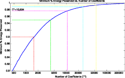
Figure 1: Compression plot: Plot of minimum proportion of energy preserved for EACH image vs. number of wavelet coefficients ($T^{*}$) for example 2-DE data set.

Image-based modeling using ISO-FMM. We constructed an isomorphic transformation for the images based on a square nonseparable 2D wavelet transform using a Daubechies wavelet with four vanishing moments, periodic boundary conditions, and the decomposition completed to $J=6$ frequency levels. To investigate image compression, we generated a compression plot (Figure 1) as described in Section 3.5. Note that we were able to preserve a high level of energy while retaining a small proportion of coefficients. The top panels of Figure 2 contain plots of one of the processed 2D gel images (uncompressed and compressed using $P=0.99,0.975\mbox{ and }0.95$) to demonstrate that the compressed and uncompressed images look virtually identical. We chose $P=0.975$ for our primary analyses, which modeled the $T=646\times 861=556{,}206$ pixels using only $T_{97.5}^{*}=10{,}634$ wavelet coefficients, for a compression ratio of more than 50:1. As a sensitivity analysis, we also ran ISO-FMM with compression levels $P=0.95$ and $P=0.99$, yielding $T_{95}^{*}=4958$ and $T_{99}^{*}=26{,}520$ coefficients, respectively, which correspond to compression ratios of over 100:1 and 20:1. We also considered the rectangular transform, but found this was not as efficient in representing the 2-DE images, with 11,384 coefficients required using $P=0.975$, so we chose to use the square transform in our analyses.

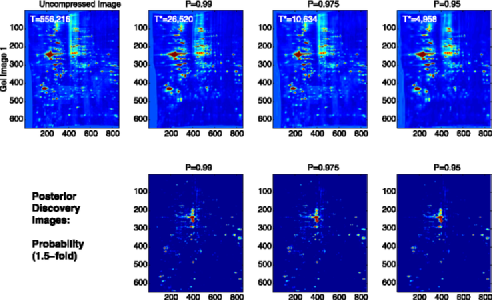
Figure 2: Illustration of compression: Heatmap of a raw uncompressed gel image and corresponding compressed images with $P=0.99,0.975$ and $0.95$ (top), along with corresponding posterior discovery images (posterior probability of 1.5-fold expression, bottom) for differences between animals in control and long cocaine access groups.

Let $Y_{i}(t_{1},t_{2}),i=1,\ldots,53$, be the $\log_{2}$-transformed preprocessed gel images. We used the following functional mixed model for these data:

$$Y_{i}(t_{1},t_{2})=\sum_{a=1}^{3}X_{ia}B_{a}(t_{1},t_{2})+\sum_{b=1}^{21}Z_{ib}U_{b}(t_{1},t_{2})+E_{i}(t_{1},t_{2}),$$ (7)

where $X_{ia}=1$ if gel $i$ is from an animal in group $a$, 0 otherwise, with the groups labeled as $a=1$ control animals, $a=2$ animals with short access to cocaine, and $a=3$ animals with long access to cocaine. The fixed effect image $B_{a}(t_{1},t_{2})$ represents the average gel for group $a$. The random effects were included to model correlation between gels from the same animal, with $Z_{ib}=1$ if gel $i$ is from animal $b$, and $U_{b}(t_{1},t_{2})$ as the random effect image for animal $b$. We assumed the random effect functions and residual error functions were i.i.d. ($P=R=I$).

After transforming the images to the wavelet space, we fit the wavelet-space version of (7) as described in Section 3.3. Maximum likelihood estimates were used for starting values of the MCMC, and vague, proper inverse gamma priors were assumed for the variance components, centered on the ML estimates with information equivalent to a sample size of $2$. After a burn-in of 1000, we ran the MCMC for 20,000 samples, keeping every 10th observation. Run on a single Xeon 2.66 GHz processor, this analysis took a total of 16.8 hours when run with $P=0.975$ compression, and 10.8 and 34.8 hours, respectively, when run with $P=0.95$ and $P=0.99$ compressions. Because the method is roughly linear in $T^{*}$, the number of basis coefficients modeled [Herrick and Morris (2006)] had we not used compression, this method would have taken approximately 600 hours using a single processor to obtain the same number of posterior samples. We note that parallel processing on a network or cluster could have been used to greatly reduce the run time. Using the 2D-$\operatorname{IDWT}$, the posterior samples of the fixed effects in the transformed space were projected back into the data space to yield posterior samples of the fixed effect images $B_{a}(t_{1},t_{2})$.

Next, we constructed posterior samples for the overall mean gel image, $M(t_{1},t_{2})=1/3\{B_{1}(t_{1},t_{2})+$ $B_{2}(t_{1},t_{2})+B_{3}(t_{1},t_{2})\}$, and to consider contrasts corresponding to the various between-group comparisons. Here we focus on the image corresponding to the difference between the control group and the long cocaine access group, $C_{13}(t_{1},t_{2})=B_{1}(t_{1},t_{2})-B_{3}(t_{1},t_{2})$ (upper right panel of Figure 4). Regions of $C_{13}(t_{1},t_{2})$ with large negative values correspond to regions with greater protein expression for animals given a long access to cocaine. Regions with large positive values correspond to regions with greater protein expression for the control animals. Using the approach described in Section 3.4, we sought to identify regions of the gel with at least 1.5-fold difference between groups [$\delta=\mbox{log}_{2}(1.5)=0.5850$], while controlling the FDR at $\alpha=0.10$.

Spot-based modeling using Pinnacle. To compare our ISO-FMM image-based approach with a standard spot-based method, we applied Pinnacle [Morris, Clark and Gutstein (2008)] to these data. First, we aligned and preprocessed the images, exactly as described above, to make sure that any difference in results was not due to preprocessing but due to the spot vs. image-based approach. Applying Pinnacle, we computed the raw mean processed gel, and denoised it using an undecimated wavelet-based approach. We detected spots based on their pinnacles, defined as any pixel that is a local maxima in both the horizontal and vertical directions of the wavelet-denoised average gel whose normalized intensity is greater than the $75$th percentile on the gel. Using the Pinnacle graphical user interface, we hand-edited the spot detection to remove obvious artifacts, and were left with a total of 752 detected spots. For each gel, we quantified each spot using the maximal normalized intensity within a $5\times 5$ square around the detected pinnacle, and then averaged intensities over replicate gels from the same animal, yielding a $21\times 752$ matrix containing normalized spot quantifications for each of 752 detected spots for the 21 animals. Using this matrix, we performed $t$-tests for each pinnacle to compare the samples from animals in the control and long cocaine access groups, and then forwarded the $p$-values into the fdrtool method [Strimmer (2008)] to obtain the corresponding $q$-values, or local false discovery rates.

4.2 Results

Results of ISO-FMM image-based analysis. First, to assess whether the model was flexible enough to model the 2-DE data, we generated a “virtual gel” by sampling from the posterior predictive distribution for the specified ISO-FMM (7), plotted in the right panel of Figure 3 along with an actual gel (left panel). The virtual gel looks remarkably like a real gel, indicating the ISO-FMM with square 2D wavelet-based modeling is able to capture the salient features of the gel, and demonstrating the flexibility of this nonparametric modeling approach.

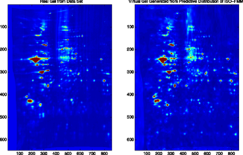
Figure 3: Virtual Gel Plot of single gel from data example (left panel) and a virtual gel (right panel), found by sampling randomly from the posterior predictive distribution of the ISO-FMM used to fit the sample data. Note that the ISO-FMM is able to sufficiently capture the structure of real 2D gels so that the virtual gel looks very much like a real gel that could have come from the example data set.

Figure 4 summarizes the overall results of the ISO-FMM model fitting. The top panels contain the posterior means for the overall mean gel image $M(t_{1},t_{2})$ and the control vs. long access contrast image $C_{13}(t_{1},t_{2})$. In the contrast image, blue regions correspond to regions of the gel with higher protein expression for animals in the long cocaine access group; red and orange regions indicate higher protein expression for control animals; and yellow regions indicate no difference. Note that we see a mix of blue and red regions, and most of these regions resemble protein spots. This is what we would expect to see in well-run gel studies with differentially expressed protein spots. If most of the effects were all in the same direction (blue or red), or if the regions were irregular and not spot shaped, then we might suspect that the results were driven by some artifacts in the data, for example, background artifacts, which might indicate a problem in the experiment.

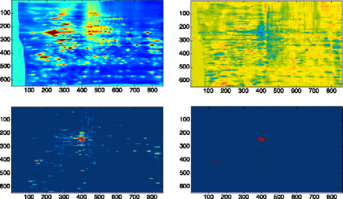
Figure 4: ISO-FMM results: Heatmaps of posterior mean of overall mean gel [$M(t_{1},t_{2})$, upper left] and control vs. long cocaine access effect gel [$C_{13}(t_{1},t_{2})$, upper right], plus probability discovery plot [$p^{1.5}(t_{1},t_{2})$, lower left] and regions of gel flagged as significant (FDR${}<0.10$, 1.5-fold, lower right). Higher intensities are indicated by hotter colors, lower intensities by cooler colors.

The bottom left panel of Figure 4 is the probability discovery plot, $p_{13}^{1.5}(t_{1},\break t_{2})$, measuring the posterior probability of at least 1.5-fold expression differences between animals in the control and long cocaine access groups with red regions having the highest posterior probabilities. The bottom panels of Figure 2 contain this probability discovery plot for the different compression levels, and demonstrate that the results are robust to the choice of compression level ${\mathcal{P}}$. Again, these regions of high probability are shaped like protein spots, as we would expect if they were marking differentially expressed proteins. Applying the FDR${}<0.10$ criterion as described in Section 3.4, we flagged all pixels $(t_{1},t_{2})$ with $p_{13}^{1.5}(t_{1},t_{2})>\phi^{1.5}_{0.10}=0.757$ as differentially expressed. These regions are marked in red in the bottom right panel of Figure 4. There are 27 contiguous regions flagged, which are summarized in Table 1. This image could be used to inform the spot-picker which physical regions of the gel to cut out for MS–MS analysis to ascertain the corresponding protein identities. Unfortunately, for this study, the original physical gels were no longer available, so we could not perform the experiment to discern the corresponding protein identities.

Table 1: Results of image-based ISO-FMM analysis: Details for regions flagged as differentially expressed in image-based ISO-FMM analysis, including coordinates of center of region ($x_{\mathrm{FMM}},y_{\mathrm{FMM}}$), maximum posterior probability of 1.5-fold change within region ($p_{1.5}$), coordinates of nearest detected pinnacle ($x_{\mathrm{Pinn}},y_{\mathrm{Pinn}}$) and corresponding p-value (pval) and fold-change (FC)

$\bolds{x_{\mathrm{FMM}}}$	$\bolds{y_{\mathrm{FMM}}}$	$\bolds{p_{1.5}}$	$\bolds{x_{\mathrm{\mathrm{Pinn}}}}$	$\bolds{y_{\mathrm{Pinn}}}$	pval	FC	Comments
403	263	${>}0.9995$	406	264	$0.0004$	2.6932	Found by both methods
415	257	${>}0.9995$	418	257	$0.0003$	2.1518	Found by both methods
410	239	${>}0.9995$	410	239	$0.0220$	1.8648	Found by both methods
393	239	$0.9995$	393	239	$0.0008$	2.1049	Found by both methods
401	252	$0.9995$	405	252	$0.0001$	1.7319	Found by both methods
386	290	$0.9890$	381	291	$0.0062$	2.2087	Found by both methods
405	483	$0.9785$	407	483	$0.0017$	1.7544	Found by both methods
398	291	$0.9150$	407	296	$0.0015$	1.5016	Found by both methods
405	203	$0.8660$	405	203	$0.0025$	1.8578	Found by both methods
391	360	$0.8240$	389	360	$0.0009$	1.8170	Found by both methods
343	227	$0.8210$	341	228	$0.0796$	1.8084	Found by both methods
712	279	$0.8035$	711	282	$0.0168$	1.5134	Found by both methods
727	278	$0.7590$	728	280	$0.0103$	1.9038	Found by both methods
831	557	$0.8925$	835	575	$0.0013$	1.4495	Fold change too small
399	220	$0.8865$	402	222	$0.0036$	1.4560	Fold change too small
109	560	$0.8630$	120	559	$0.0167$	1.2412	Fold change too small
232	639	$0.8560$	240	639	$0.0087$	1.4723	Fold change too small
797	540	$0.8210$	799	541	${<}0.0001$	1.4866	Fold change too small
388	335	$0.7820$	383	333	${<}0.0001$	1.4096	Fold change too small
832	351	$0.8540$	828	357	$0.1466$	1.2377	In right tail of major spot
762	238	$0.8375$	773	243	$0.7220$	1.0500	In left tail of major spot
144	408	$0.9815$	160	409	$0.9883$	1.0011	In left tail of major spot
154	427	$0.9775$	177	427	$0.3312$	1.0477	In left tail of major spot
704	332	$0.8795$	713	338	$0.4748$	1.0767	In left tail of major spot
559	222	$0.9420$	562	220	$0.4697$	1.0558	Between two visible spots
449	251	$0.8940$	446	257	$0.1105$	1.2458	Between two visible spots
308	175	$0.7985$	312	172	$0.0471$	1.3055	Between two visible spots

Results of Pinnacle spot-based analysis. Performing a spot-based analysis, we flagged a spot as significant if its $q$-value was less than 0.10, and the effect size was at least $\log_{2}(1.5)=0.5850$, indicating at least 1.5-fold difference. This led to 17 differentially expressed spots between animals in the control and long cocaine access groups, which are summarized in Table 2.

Table 2: Results of spot-based Pinnacle analysis: Details for spots flagged as differentially expressed in spot-based Pinnacle analysis, including location ($x$, $y$), $p$-value (pval), $q$-value (qval) and fold-change (FC). Also included is the maximum $p_{1.5}(t_{1},t_{2})$ from the ISO-FMM within a 5-by-5 neighborhood around the corresponding Pinnacle

$\bolds{x}$	$\bolds{y}$	pval	qval	FC	$\bolds{p_{1.5}}$	Comments
410	$239$	$0.002$	0.008	1.865	${>}0.999$	Found by both methods
418	$257$	${<}0.001$	0.002	2.152	${>}0.999$	Found by both methods
406	$264$	${<}0.001$	0.003	2.693	${>}0.999$	Found by both methods
405	$252$	${<}0.001$	0.001	1.732	$0.999$	Found by both methods
393	$239$	$0.001$	0.004	2.105	$0.999$	Found by both methods
381	$291$	$0.006$	0.014	2.209	$0.989$	Found by both methods
407	$483$	$0.002$	0.007	1.754	$0.979$	Found by both methods
407	$203$	$0.005$	0.013	1.671	$0.866$	Found by both methods
389	$360$	$0.001$	0.005	1.817	$0.824$	Found by both methods
341	$228$	$0.080$	0.068	1.808	$0.821$	Found by both methods
711	$282$	$0.017$	0.027	1.513	$0.804$	Found by both methods
407	$296$	$0.001$	0.007	1.502	$0.788$	Found by both methods
728	$281$	$0.014$	0.024	1.638	$0.759$	Found by both methods
379	$263$	$0.009$	0.018	1.595	$0.487$	Just missed threshold
257	$60$	$0.062$	0.048	1.663	$0.463$	Just missed threshold
409	$163$	$0.006$	0.014	1.504	$0.160$	FC barely above 1.5
798	$177$	$0.004$	0.012	1.543	$0.019$	FC barely above 1.5, faint spot

Comparison of Pinnacle and ISO-FMM results. Note that the Pinnacle and ISO-FMM results are not entirely comparable since they use different criteria; Pinnacle flags a spot as significant if the $q$-value is less than 0.10 (based on a $t$-test with point mass null hypothesis) and the effect size is at least 1.5-fold, while the ISO-FMM flags a region as significant if its posterior probability of a 1.5-fold difference is large enough to cross the estimated $\mathit{FDR}<0.10$ significance threshold. However, we still found it enlightening to qualitatively compare these results.

Out of the 17 spots flagged as significant by Pinnacle, 13 were contained within regions flagged by the ISO-FMM analysis. Two of the others have high probabilities of 1.5-fold difference (${\approx}0.50$), but that just missed the $\mathit{FDR}<0.10$ threshold of $\phi^{1.5}_{10}=0.757$. The other two were very faint spots with fold changes marginally greater than 1.5-fold.

Of the 27 regions flagged in the ISO-FMM analysis, 13 have corresponding pinnacle results. Figure 5 displays one such region, marked by the small box in Figure 4. We see that this region precisely corresponds to the boundaries of a single visible spot, and the Pinnacle location is marked by the “$\times$,” with the “o” indicating it was flagged as significant by the Pinnacle spot-based analysis. Six more regions clearly correspond to visible spots in the mean gel that have small $p$-values, but estimated fold-changes less than 1.5. The remaining 8 nonmatched regions corresponded to subsets of detected spots or in the areas between two spots; four corresponded to regions in the left tail of visible spot, one to a region in the right tail of a visible spot, and the remaining three appeared between 2 visible spots. These results were not found by the spot-based Pinnacle approach.

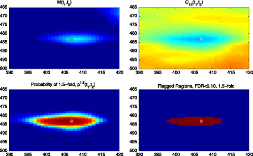
Figure 5: Specific Results 1: Posterior mean of overall mean gel (upper left), effect gel (upper right), probability discovery plot (lower left), and indicating ISO-FMM flagged regions (lower right) for region marked by small box in Figure 4, with pinnacles for detected spots marked ($\times$), and differential expression in Pinnacle analysis indicated by a (o). Note that region flagged by ISO-FMM corresponds to visible spot also detected by Pinnacle analysis.

One interesting part of the gel containing two such regions is indicated by the large box in Figure 4, and presented in detail in Figure 6. From the mean gel image, we see that this field contains 7 visible protein spots detected by Pinnacle, as marked by the $\times$’s. From the other panels, we see two regions flagged as differentially expressed (long access${}>{}$control) by ISO-FMM, and a third region with high probability of differential expression but not quite exceeding the $\mathit{FDR}=0.10$ threshold $\phi^{1.5}_{0.10}=0.757$. These flagged regions resemble protein spots but do not correspond to the visible protein spots in the mean gel. Rather, they correspond to the left tails of the two dominant spots in this field, which both appear to have slightly extended long tails. The spot-based approach found no significant spots in this region of the gel, so these discoveries would have been missed had we not conducted the image-based analysis. Other spots have similar behavior, and their details can be seen in supplementary Figures 3–10 [Morris (2010)]. A key question is what these flagged regions could represent.

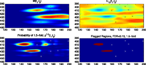
Figure 6: Specific Results 2: Posterior mean of overall mean gel (upper left), effect gel (upper right), probability discovery plot (lower left), and indicating ISO-FMM flagged regions (lower right) for region marked by large box in Figure 4, with pinnacles for detected spots marked ($\times$), and differential expression in Pinnacle analysis indicated by a (o). Note that regions flagged by ISO-FMM correspond to tails of visible spots that themselves are not differentially expressed. These results are not found by the Pinnacle analysis.

Interpretation of results. As mentioned in Section 2, a well-known issue in 2-DE is the presence of co-migrating proteins, that is, distinct proteins that visually appear to be part of the same protein spot. Studies have shown that some spots on a gel can have as many as 5 or 6 distinct proteins [Gygi et al. (2000)]. These co-migrating proteins can be different proteins or post-translational modifications of the same protein, which can also be functionally distinct. If two proteins have similar combinations of pH and molecular mass, it is possible that the proteins will run together in the same visible spot on the 2-DE. It can be very difficult, and sometimes impossible, for any spot detection method to deconvolve these multiple spots into separate protein spots, especially if one of them has considerably higher abundance than the others. The inability to resolve these co-migrating proteins is one of the key criticisms levied against 2-DE. The significant regions flagged by ISO-FMM but not by Pinnacle which appear in the tail of a visible spot or between two visible spots may indicate differentially expressed co-migrating proteins visibly masked by a more abundant non differentially-expressed protein, and that these proteins were completely missed by the spot-based analysis. Studies are underway to confirm this possibility.

In this way, the image-based modeling approach may be able to extract more protein information from the gels than spot-based approaches. Because spot-based modeling approaches have been almost universally used to date, this means that perhaps 2-DE contains more proteomic information than was previously known. The image-based approach may effectively increase the realized resolution of the gels and better extract the proteomic information they contain. Further biological studies are needed to validate these conjectures.

5 Discussion

In this paper we have discussed a general Bayesian method for quantitative image data based on functional mixed models that uses an isomorphic modeling approach. The underlying FMM framework is very general, can simultaneously model any number of covariates, each having their own fixed effect image of general form, and can account for correlation between the images using random effect images and between-image covariance matrices. The results from the method can be used to perform FDR-based Bayesian inference that takes both practical and statistical significance into account, and flags significant regions of the fixed effect images.

Previous work on functional mixed models has been limited to single-dimensional functions; here we have shown how this approach can be applied to images of dimension 2 or higher. Also, previous work on functional mixed models has been based on specific modeling strategies using smoothing splines [Guo (2002)] or wavelets [Morris and Carroll (2006)]. In this paper we have described a general modeling strategy that involves using an isomorphic transformation to map the data to an alternative space, where modeling can be done more parsimoniously and smoothing or regularization naturally done, and results can be mapped back to the original data space for final inference. This method, ISO-FMM, contains WFMM as a special case, but can be also applied much more generally using other isomorphic transformations. With each proposed transformation, careful thought needs to be given to the modeling choices and their implications in the data space, and thus further work is required to apply this approach using certain other transformations. This general modeling strategy can be used for the 1D FMM, or for the higher dimensional FMM that is the primary interest of this paper. This isomorphic modeling approach is a general strategy with potential for application to a variety of other contexts.

We introduced a compression method to reduce the dimensionality of the data that is appropriate when the chosen isomorphic transformation leads to a sparse representation for all of the images, as is true for wavelets. This compression method can also be applied to any functional data, 1-D or higher. We have found it is possible to use compression to speed up the computations by one or two orders of magnitude, which greatly reduces the memory overhead requirements without substantively changing the results.

While the method is complex, we have developed general freely available software (http://biostatistics.mdanderson.org/SoftwareDownload/SingleSoftware.aspx?Software_Id=70) to implement it that is efficient enough to handle very large data sets and complex models, and is relatively straightforward to use, considering the complexity of the method. If the user is satisfied with automatic vague proper priors and default wavelet bases, then the method can run completely automatically if the user simply specifies the $Y$, $X$ and $Z$ matrices. Users who wish to use alternative basis functions can compute the $D$ matrix themselves and feed that into the program, indicating which groups of coefficients will share common smoothing parameters. The code automatically generates posterior means and quantiles (default 0.005, 0.01, 0.025, 0.975, 0.99, 0.995) for prespecified contrasts involving the $B_{a}(t_{1},t_{2})$, plus the posterior probabilities of specific effect sizes $p^{\delta}_{a}(t_{1},t_{2})$ for specified choices of $\delta$ {default $\delta=\log_{2}(1.25),\log_{2}(1.5),\log_{2}(2.0)$}. Thus, plots like those generated in Figure 4 can be quickly generated once the method is run. The code is continually being updated as the scope of the FMM framework is extended, so more features will be added in the future, as will an R interface for running the method.

Applying this method to 2-DE data, we found that the ISO-FMM was able to find differentially expressed proteins that may be co-migrating proteins that would not have been found using the usual spot-based analysis approaches. The ISO-FMM may be capable of extracting more proteomic information from the gels than was previously known to be there. This method can easily be applied to DIGE data by just modeling $Y_{i}(t_{1},t_{2})$ to be the log ratio of the two channels. Although this paper focused on 2-DE, the ISO-FMM can be applied to any type of quantitative image data, including fMRI, LC–MS and other commonly encountered applications. This rigorous, automated method can be useful in extracting information and performing inference for quantitative image data.

References

- (1) Ahmed, S. H. and Koob, G. F. (1998). Transition from moderate to excessive drug intake: Change in hedonic set point. Science 282 298–300.
- (2) Benjamini, Y. and Hochberg, Y. (1995). Controlling the false discovery rate: A practical and powerful approach to multiple testing. J. Roy. Statist. Soc. Ser. B 57 289–300. \MR1325392
- (3) Candes, E. J. and Donoho, D. L. (2000). Curvelets, multiresolution representation, and scaling laws. In SPIE Wavelet Applications in Signal and Image Processing VIII (A. Aldroubi, A. F. Laine and M. A. Unser, eds.). Proc. SPIE 4119. Hindawi, New York.
- (4) Clark, B. N. and Gutstein, H. B. (2008). The myth of automated, high-throughput two-dimensional gel electrophoresis. Proteomics 8 1197–1203.
- (5) Clyde, M., Parmigiani, G. and Vidakovic, B. (1998). Multiple shrinkage and subset selection in wavelets. Biometrika 85 391–401. \MR1649120
- (6) Dawid, A. P. (1981). Some matrix-variate distribution theory: Notational considerations and a Bayesian application. Biometrika 68 265–274. \MR0614963
- (7) Diggle, P. J. and Al Wasel, I. (1997). Spectral analysis of replicated biomedical time series. J. Roy. Statist. Soc. Ser. C 46 31–71. \MR1452286
- (8) Do, M. N. and Vetterli, M. (2001). Beyond Wavelets (J. Stoeckler and G. V. Welland, eds.). Academic Press, New York. \MR2136835
- (9) Do, M. N. and Vetterli, M. (2005). The contourlet transform: An efficient directional multiresolution image representation. IEEE Trans. Image Process. 14 2091–2106.
- (10) Dowsey, A. W., Dunn, M. J. and Yang, G. Z. (2008). Automated image alignment for 2D gel electrophoresis in a high-throughput proteomics pipeline. Bioinformatics 24 950–957.
- (11) Faergestad, E. M., Rye, M., Walczak, B., Gidskehaug, L., Wold, J. P., Grove, H., Jia, X., Hollung, K., Indahl, U. G., Westad, F., van den Berg, F. and Martens, H. (2007). Pixel-based analysis of multiple images for the indentification of changes: A novel approach applied to unravel patterns of 2-D electrophoresis gel images. Proteomics 7 3450–3461.
- (12) Feilner, M., Van De Ville, D. and Unser, M. (2005). An orthogonal family of quincunx wavelets with continuously adjustable order. IEEE Trans. Signal Process. 14 499–510. \MR2128291
- (13) Gygi, S. P., Corthals, G. L., Zhang, Y., Rochon, Y. and Aebersold, R. (2000). Evaluation of two-dimensional gel electrophoresis-based proteome analysis technology. Proc. Natl. Acad. Sci. USA 97 9390–9395.
- (14) Guo, W. (2002). Functional mixed effects models. Biometrics 58 121–128. \MR1891050
- (15) Heinrichs, S. C., Menzaghi, F., Schulteis, G., Koob, G. F. and Stinus, L. (1995). Suppression of corticotropin-releasing factor in the amygdala attenuates aversive consequences of morphine withdrawal. Behavioral Pharmacology 6 74–80.
- (16) Herrick, R. C. and Morris, J. S. (2006). Wavelet-based functional mixed model analysis: Computational considerations. In Proceedings, Joint Statistical Meetings, ASA Section on Statistical Computing 2051–2053. Amer. Statist. Assoc., Alexandria, VA.
- (17) Karp, N. A. and Lilley, K. S. (2005). Maximizing sensitivity for detecting changes in protein expression: Experimental design using minimal CyDyes. Proteomics 5 3105–3115.
- (18) Kokkinidis, L., Zacharko, R. M. and Predy, P. A. (1980). Post-amphetamine depression of self-stimulation responding from the substantia nigra: Reversal by tricyclic antidepressants. Pharmacol Biochem. Behav. 12 379–383.
- (19) Leith, N. J. and Barrett, R. J. (1976). Amphetamine and the reward system: Evidence for tolerance and post-drug depression. Psychopharmacologia 46 19–25.
- (20) Lilley, K. S. (2003). Protein profiling using two-dimensional difference gel electrophoresis (2-D DIGE). In Current Protocols in Protein Science, Chapter 22, Unit 22.2. Wiley, New York.
- (21) Mallat, S. G. (1989). A theory for multiresolution signal decomposition: The wavelet representation. IEEE Trans. Pattern Anal. Mach. Intell. 11 674–693.
- (22) Markou, A. and Koob, G. (1992). Bromocriptine reverses the elevation in intracranial self-stimulation thresholds observed in a rat model of cocaine withdrawal. Neuropsychopharmacology 7 213–224.
- (23) Morris, J. S. (2010). Supplement to “Automated analysis of quantitative image data using isomorphic functional mixed models, with application to proteomics data.” DOI: 10.1214/10-AOAS407SUPPA, DOI: 10.1214/10-AOAS407SUPPB, DOI: 10.1214/10-AOAS407SUPPC, DOI: 10.1214/10-AOAS407SUPPD.
- (24) Morris, J. S., Arroyo, C., Coull, B., Ryan, L. M., Herrick, R. and Gortmaker, S. L. (2006). Using wavelet-based functional mixed models to characterize population heterogeneity in accelerometer profiles: A case study. J. Amer. Statist. Assoc. 101 1352–1364. \MR2307570
- (25) Morris, J. S., Brown, P. J., Herrick, R. C., Baggerly, K. A. and Coombes, K. R. (2008). Bayesian analysis of mass spectrometry data using wavelet-based functional mixed models. Biometrics 12 479–489. \MR2432418
- (26) Morris, J. S. and Carroll, R. J. (2006). Wavelet-based functional mixed models. J. Roy. Statist. Soc. Ser. B 68 179–199. \MR2188981
- (27) Morris, J. S., Clark, B. N. and Gutstein, H. B. (2008). Pinnacle: A fast, automatic and accurate method for detecting and quantifying protein spots in 2-dimensional gel electrophoresis data. Bioinformatics 24 529–536.
- (28) Morris, J. S., Vannucci, M., Brown, P. J. and Carroll, R. J. (2003). Wavelet-based nonparametric modeling of hierarchical functions in colon carcinogenesis. J. Amer. Statist. Assoc. 98 573–583.
- (29) Morris, J. S., Clark, B. N., Wei, W. and Gutstein, H. B. (2010). Evaluting the performance of new approaches to spot quantification and differential expression in 2-dimensional gel electrophoresis studies. Journal of Proteome Research 9 595–604.
- (30) Mueller, P., Parmigiani, G., Robert, C. and Rousseau, J. (2004). Optimal sample size for multiple testing: The case of gene expression microarrays. J. Amer. Statist. Assoc. 99 990–1001. \MR2109489
- (31) Parsons, L. H., Koob, G. F. and Weiss, F. (1995). Serotonin dysfunction in the nucleus accumbens of rats during withdrawal after unlimited access to intravenous cocaine. Journal of Pharmacology and Experimental Therapeutics 274 1182–1191.
- (32) Ramsay, J. O. and Silverman, B. W. (1997). Functional Data Analysis. Springer, New York. \MR2168993
- (33) Reiss, P. T. and Ogden, R. T. (2009). Functional generalized linear models with images as predictors. Biometrics. Published online May 8, 2009.
- (34) Richter, R. and Weiss, F. (1999). In vivo CRF release in rat amygdala is increased during cocaine withdrawal in self-administering rats. Synapse 32 254–261.
- (35) Sampson, P. D. and Guttorp, P. (1992). Nonparametric estimation of nonstationary spatial covariance structure. J. Amer. Statist. Assoc. 87 108–119.
- (36) Schulteis, G., Markou, A., Gold, L. H., Stinus, L. and Koob, G. F. (1994). Relative sensitivity to naloxone of multiple indices of opiate withdrawal: A quantitative dose–response analysis. Journal of Pharmacology and Experimental Therapeutics 271 1391–1398.
- (37) Smith, M. and Fahrmeir, L. (2007). Spatial Bayesian variable selection with application to functional magnetic resonance imaging. J. Amer. Statist. Assoc. 102 417–431. \MR2370843
- (38) Storey, J. D. (2003). The positive false discovery rate: A Bayesian interpretation and the -value. Ann. Statist. 31 2013–2035. \MR2036398
- (39) Strimmer, K. (2008). fdrtool: A versitile R package for estimating local and tail area-based false discovery rates. Bioinformatics 24 1461–1462.
- (40) Weiss, F., Markou, A., Lorang, M. T. and Koob, G. F. (1992). Basal extracellular dopamine levels in the nucleus accumbens are decreased during cocaine withdrawal after unlimited-access self-ad ministration. Brain Research 593 314–318.