Beating the efficiency of both quantum and classical simulations with semiclassics

Abstract

While rigorous quantum dynamical simulations of many-body systems are extremely difficult (or impossible) due to the exponential scaling with dimensionality, corresponding classical simulations completely ignore quantum effects. Semiclassical methods are generally more efficient but less accurate than quantum methods, and more accurate but less efficient than classical methods. We find a remarkable exception to this rule by showing that a semiclassical method can be both more accurate and faster than a classical simulation. Specifically, we prove that for the semiclassical dephasing representation the number of trajectories needed to simulate quantum fidelity is independent of dimensionality and also that this semiclassical method is even faster than the most efficient corresponding classical algorithm. Analytical results are confirmed with simulations of quantum fidelity in up to $100$ dimensions with $2^{1700}$-dimensional Hilbert space.

Introduction. Correct description of many microscopic dynamical phenomena, such as ultrafast time-resolved spectra or tunneling rate constants, requires an accurate quantum (QM) simulation. While classical (CL) molecular dynamics simulations are feasible for millions of atoms, solution of the time-dependent Schrödinger equation scales exponentially with the number $D$ of degrees of freedom (DOF) and is feasible for only a few continuous DOF. An apparently promising solution is provided by semiclassical (SC) methods, which use CL trajectories, but attach to them phase information, and thus can approximately describe interference and other QM effects completely missed in CL simulations. Unfortunately, SC methods suffer from the “dynamical sign problem” due to the addition of rapidly oscillating terms, resulting in the requirement of a huge number of CL trajectories for convergence. Consequently, most SC methods are much less efficient than CL simulations and in practice were used for at most tens of DOF. Even though several techniques have explored this issue Walton and Manolopoulos (1996); *kay:1994a; *sklarz:2004; *wang:1998; *tatchen:2011; *tao:2011; *vanicek:2001; *vanicek:2003, the challenge remains open. Below we turn this challenge around by showing that in simulations of QM fidelity (QF) Gorin et al. (2006); Jacquod and Petitjean (2009), a SC method called “dephasing representation” (DR) is not only more accurate but, remarkably, also faster than the most efficient corresponding CL algorithm Mollica et al. .

Quantum and classical fidelity. QF was introduced by Peres Peres (1984) to measure the stability of QM dynamics (QD). He defined QF $F_{\text{QM}}(t)$ as the squared overlap at time $t$ of two QM states, identical at $t=0$, but subsequently evolved with two different Hamiltonians, $H_{0}$ and $H_{\epsilon}=H_{0}+\epsilon V$:

$$F_{\text{QM}}(t) :=\left|f_{\text{QM}}(t)\right|^{2},$$ (1)

$$f_{\text{QM}}(t) :=\langle\psi\left|U_{\epsilon}^{-t}U_{0}^{t}\right|\psi\rangle,$$ (2)

where $f_{\text{QM}}(t)$ is the fidelity amplitude and $U_{\epsilon}^{t}:=\exp(-iH_{\epsilon}t/\hbar)$ the QM evolution operator. Rewriting Eq. (2) as $f_{\text{QM}}(t)=\langle\psi\left|U^{t}\right|\psi\rangle$ with the echo operator $U^{t}:=U_{\epsilon}^{-t}U_{0}^{t}$, it can be interpreted as the Loschmidt echo, i.e., an overlap of an initial state with a state evolved for time $t$ with $H_{0}$ and subsequently for time $-t$ with $H_{\epsilon}$. (In general, we write time $t$ as a superscript. Subscript $\epsilon$ denotes that $H_{\epsilon}$ was used for dynamics. If an evolution operator, phase space coordinate, or density lacks a subscript $\epsilon$, Loschmidt echo dynamics is implied.) QF amplitude (2) is ubiquitous in applications: it appears in NMR spin echo experiments Pastawski et al. (2000), neutron scattering Petitjean et al. (2007), ultrafast electronic spectroscopy Mukamel (1982); *rost:1995; *li:1996; *egorov:1998; *shi:2005; Wehrle et al. (2011), etc. QF (1) is relevant in QM computation and decoherence Cucchietti et al. (2003); *gorin:2004, and can be used to measure nonadiabaticity Zimmermann and Vaníček (2010); *zimmermann:2011 or accuracy of molecular QD on an approximate potential energy surface Li et al. (2009); *zimmermann:2010c.

Definition (1) can be generalized to mixed states in different ways Gorin et al. (2006); Vaníček (2004, , 2006), but we assume that the initial states are pure. In this case, one may write QF (1) as $F_{\text{QM}}(t)=\operatorname{Tr}\left(\hat{\rho}_{\epsilon}^{t}\hat{\rho}_{0}^{t}\right)$ where $\hat{\rho}_{\epsilon}^{t}:=U_{\epsilon}^{t}\hat{\rho}U_{\epsilon}^{-t}$ is the density operator at time $t$. In the phase-space formulation of QM mechanics, QF becomes $F_{\text{QM}}(t)={h}^{-{D}}\int dx\rho_{\epsilon,{\text{W}}}^{t}(x)\rho_{0,{\text{W}}}^{t}(x)$ where $x:=\left(q,p\right)$ is a point in phase space and $A_{\text{W}}(x):=\int d\xi\langle q-\xi/2\left|\hat{A}\right|q+\xi/2\rangle e^{ip\xi/\hbar}$ is the Wigner transform of $\hat{A}$. This form of QF suggests its CL limit, called CL fidelity (CF) Prosen and Žnidarič (2002); Benenti and Casati (2002)

$$F_{\text{CL}}(t) :=F_{\text{fid}}(t)=h^{-D}\int dx\rho_{\epsilon}^{t}(x)\rho_{0}^{t}(x)$$ (3)

$$=F_{\text{echo}}(t)={h}^{-{D}}\int d{x}\rho^{t}(x)\rho^{0}(x)$$ (4)

where the first and second line express CF in the fidelity and Loschmidt echo pictures, respectively. If $F$ or $\rho$ lack the subscript “CL”, “QM”, or “DR”, “CL” is implied.

Dephasing representation. There were several attempts at describing QF semiclassically. Most were analytical Jalabert and Pastawski (2001); *cohen_kottos:2000; *cerruti:2002; Jacquod and Petitjean (2009) and valid only under special circumstances because the numerical approaches were overwhelmed with the sign problem. Extending a numerical SC method for localized Gaussian wavepackets (GWPs) Vaníček and Heller (2003), the DR was introduced as a more accurate and general approximation of QF Vaníček (2004, , 2006). The DR of QF amplitude is an interference integral

$$f_{\text{DR}}(t) :=h^{-D}\int dx^{0}\rho_{\text{W}}(x^{0})\exp[i\phi(x^{0},t)],$$ (5)

$$\phi(x^{0},t) :=-\Delta S(x^{0},t)/\hbar=\left(\epsilon/\hbar\right)\int_{0}^{t}d\tau V(x_{\epsilon/2}^{\tau}),$$ (6)

where the phase $\phi$ is determined by the action $\Delta S$ due to the perturbation along a trajectory propagated with the average Hamiltonian $H_{\epsilon/2}$ Wehrle et al. (2011); Zambrano and Ozorio de Almeida . Above, $x_{\epsilon}^{t}:=\Phi_{\epsilon}^{t}(x^{0})$ where $\Phi_{\epsilon}^{t}$ is the Hamiltonian flow of $H_{\epsilon}$ and the perturbation $V$ can, in general, depend on both $q$ and $p$. The DR of fidelity, computed as $F_{\text{DR}}:=|f_{\text{DR}}|^{2}$, was successfully used to describe stability of QD in integrable, mixed, and chaotic systems Vaníček (2004, , 2006), nonadiabaticity Zimmermann and Vaníček (2010, 2011) and accuracy of molecular QD on an approximate potential energy surface Li et al. (2009); Zimmermann et al. (2010), and the local density of states and the transition from the Fermi-Golden-Rule (FGR) to the Lyapunov regime of QF decay Wang et al. (2005); *ares:2009; *wisniacki:2010; *garcia-mata:2011b. The same approximation was independently derived and used in electronic spectroscopy Mukamel (1982); *rost:1995; *li:1996; *egorov:1998; *shi:2005. Recently, the range of validity of the DR was extended with a SC prefactor Zambrano and Ozorio de Almeida . The remarkable efficiency of the original DR observed empirically in applications led us to analyze this property rigorously here and to compare it with the efficiencies of the QM and CL calculations of QF.

Algorithms. The most general and straightforward way to evaluate Eqs. (3)-(4) and (5) is with trajectory-based methods. While the DR (5) is already in a suitable form, Eqs. (3)-(4) for CF must be rewritten using the Liouville theorem as

$$F_{\text{fid}}(t) ={h}^{-{D}}\int d{x^{0}}\rho(x_{\epsilon}^{-t})\rho(x_{0}^{-t})\text{ \ and}$$ (7)

$$F_{\text{echo}}(t) ={h}^{-{D}}\int d{x^{0}}\rho(x^{-t})\rho(x^{0}).$$ (8)

Above, $x^{t}:=\Phi^{t}(x^{0})$ where $\Phi^{t}:=\Phi_{\epsilon}^{-t}\circ\Phi_{0}^{t}$ is the Loschmidt echo flow. Since it is the phase space points rather than the densities that evolve in expressions (7)-(8), we can take $\rho=\rho_{\text{W}}^{t=0}$. For numerical computations, Eqs. (5) and (7)-(8) are further rewritten in a form suitable for Monte Carlo evaluation, i.e., as an average

$$\left\langle A(x^{0},t)\right\rangle_{W(x^{0})}:=\frac{\int d{x^{0}}A(x^{0},t)W(x^{0})}{\int d{x^{0}}W(x^{0})}$$

where $W$ is the sampling weight for initial conditions $x^{0}$. Using $W=\rho_{\text{W}}(x^{0})$, the DR algorithm becomes Vaníček (2004, , 2006)

$$f_{\text{DR}}(t)={{\left\langle\exp\left[i\phi(x^{0},t)\right]\right\rangle}_{\rho_{\text{W}}(x^{0})}}.$$ (9)

Sampling is straightforward for $\rho_{\text{W}}\geq 0$, but can be done also for general pure states Vaníček (2006). While previously used CL algorithms sampled from $W=\rho$ Benenti and Casati (2002); Karkuszewski et al. (2002); *benenti:2003; *benenti:2003a; *veble:2004; *casati:2005; *veble:2005, Ref. Mollica et al. considered more general weights $W=W_{M}(x^{0}):=\rho(x^{0})^{M}$ and $W=W_{M}(x_{0}^{-t})=\rho(\Phi_{0}^{-t}(x^{0}))^{M}$ for the echo and fidelity dynamics, respectively. These weights yield four families of $M$-dependent algorithms Mollica et al.

$$F_{\text{fid-}M}(t) =I_{M}{\langle\rho(x_{\epsilon}^{-t})\rho(}x_{0}^{-t})^{1-M}{\rangle}_{\rho(x_{0}^{-t})^{M}},$$ (10)

$$F_{\text{echo-}M}(t) =I_{M}{\langle\rho(x^{-t})\rho(}x^{0})^{1-M}{\rangle}_{\rho(x^{0})^{M}},$$ (11)

$$F_{\text{fid-N-}M}(t) =\frac{{\langle\rho(x_{\epsilon}^{-t})\rho(}x_{0}^{-t})^{1-M}{\rangle}_{\rho(x_{0}^{-t})^{M}}}{{\langle}\rho(x_{0}^{-t})^{2-M}{\rangle}_{\rho(x_{0}^{-t})^{M}}},$$ (12)

$$F_{\text{echo-N-}M}(t) =\frac{{\langle\rho(x^{-t})\rho(}x^{0})^{1-M}{\rangle}_{\rho(x^{0})^{M}}}{{\langle\rho(}x^{0})^{2-M}{\rangle}_{\rho(x^{0})^{M}}},$$ (13)

where $I_{M}:=h^{-D}\int\rho(x^{0})^{M}dx^{0}$ is a normalization factor. Conveniently, the “normalized” (N) algorithms (12)-(13) do not require the normalization factor $I_{M}$ which is, for general states, known explicitly only for $M\in\{0,1,2\}$ ($I_{0}=n_{1}^{D}$, $I_{1}=I_{2}=1$). For further details, see Ref. Mollica et al. where it was found that the echo-2 algorithm is optimal since it is already normalized (i.e., echo-2 = echo-N-2), applies to any pure state (in particular, $\rho$ does not have to be positive definite), and–most importantly–is by far the most efficient CL algorithm.

Efficiency. The reader does not have to be persuaded of the exponential scaling of QD with $D$. We just note that the direct diagonalization of the Hamiltonian leads to a QD algorithm with a cost $O(t^{0}n_{D}^{3})=O(t^{0}n_{1}^{3D})$ where $n_{D}=n_{1}^{D}$ is the dimension of the Hilbert space of $D$ DOF. Despite the independence of $t$, the scaling with $D$ is overwhelming. More practical is the split-operator algorithm requiring the fast Fourier transform (FFT) at each step. The complexity of FFT is $O(n_{D}\log n_{D})$, hence the overall cost is $O(tD{n_{1}}^{D}\log{n_{1}})$. The effective $n_{1}$ is reduced in increasingly popular methods with evolving bases, but the exponential scaling remains.

Regarding the CF and DR algorithms, efficiency of trajectory-based methods depends on two ingredients: First, what is the cost of propagating $N$ trajectories for time $t$? Second, what $N$ is needed to converge the result to within a desired discretization error $\sigma_{\text{discr}}$? As this analysis was done for the CL algorithms in Ref. Mollica et al. , here we only outline the main ideas and apply them to analyze the efficiency of the DR.

The cost of a typical method propagating $N$ trajectories for time $t$ is $O(c_{\text{f}}tN)$ where $c_{\text{f}}$ is the cost of a single force evaluation. However, among the above mentioned algorithms, this is only true for the fidelity algorithms with $M=0$ (i.e., fid-0 and fid-N-0) and for the DR! Remarkably, in all other cases, the cost is $O(c_{\text{f}}t^{2}N)$. The cost is linear in time for a single time $t$, but becomes quadratic if one wants to know CF for all times up to $t$. For the echo algorithms, it is due to the necessary full backward propagation for each time between $0$ and $t$. For the fidelity algorithms, it is because the weight function $\rho(x^{-t})^{M}$ changes with time and the sampling has to be redone for each time between $0$ and $t$ Mollica et al. .

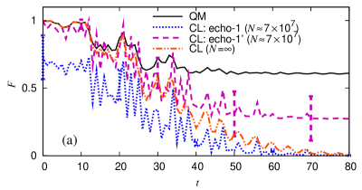
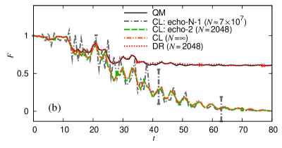
Figure 1: Convergence of different fidelity algorithms in a $100$-dimensional system of perturbed ($\epsilon=3\times 10^{-4}$) quasi-integrable ($k=0.2$) kicked rotors with $n_{1}=8192$. Error bars plotted every 20 time steps. (a) Simple algorithms echo-1 and echo-1’ are far from converged even with $7\times 10^{7}$ trajectories. (b) While both DR and echo-2 algorithms converge fully with only $2048$ trajectories, only the DR can capture the QM fidelity “freeze” (the plateau).

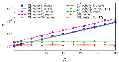
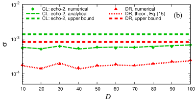
Figure 2: Statistical error grows exponentially with $D$ for the echo-1, echo-1’, and echo-N-1 algorithms, while it is independent of $D$ for the echo-2 and DR algorithms. (a) Pure displacement dynamics obtained with two displaced $D$-dimensional SHOs. $N\approx 10^{7}$. Time chosen separately for each $D$ so that $F\approx 0.3$. (b) General dynamics obtained with a $D$-dimensional system of perturbed ($\epsilon=10^{-4}$) quasi-integrable ($k=0.2$) kicked rotors with $n_{1}=131072$. $N\approx 5\times 10^{5}$. Time chosen separately for each $D$ so that $F\approx 0.9$.

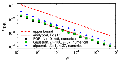
Figure 3: Regardless of dynamics, statistical error of the DR is independent of dimensionality ($D$), time ($t$), and is proportional to $N^{-1/2}$. Errors are compared for $10$ kicked rotors in the chaotic FGR regime $(k=18,\epsilon=6.4\times 10^{-6},n_{1}=131072)$, $100$ kicked rotors in the integrable Gaussian regime $(k=0.2,\epsilon=6.4\times 10^{-6},n_{1}=131072)$, and a single kicked rotor in the quasi-integrable algebraic regime $(k=0.2,\epsilon=6.4\times 10^{-4},n_{1}=131072)$. Time $t$ was chosen separately for each system so that $F\approx 0.94$.

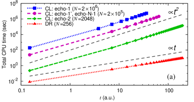
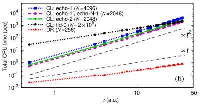
Figure 4: Computational cost as a function of simulation time $t$ for different algorithms. The CPU time grows quadratically with $t$ for all CL echo algorithms while it is only linear with $t$ for the DR and fid-0 algorithms. Dynamics is of pure displacement type given by a $D$-dimensional system of displaced SHOs for which all algorithms converge to the exact result. Fidelity was computed at fidelity revival times at which $F\approx 0.9$. Number of trajectories ($N$) was selected for each algorithm separately so that the statistical error $\sigma\approx 0.01$ for all methods. (a) $D=20$. (b) $D=1$.

The number $N$ of trajectories required for convergence can depend on $D$, $t$, dynamics, initial state, and method. Below we estimate $N$ for the DR analytically using the technique proposed in Ref. Mollica et al. . The expected systematic component of $\sigma_{\text{discr}}$ is zero for $f_{\text{DR}}$ and $O(N^{-1})$ for $F_{\text{DR}}$ and is negligible to the expected statistical component $\sigma=O(N^{-1/2})$ which therefore determines convergence. Expected statistical error of $A(N)$ is computed as $\sigma_{A}^{2}(N)={\overline{\left|A(N)\right|^{2}}-}\left|{\overline{A(N)}}\right|{{}^{2}}$ where the overline denotes an average over infinitely many independent simulations with $N$ trajectories.

The discretized form of Eq. (9) is $f_{\text{DR}}(t,N)=N^{-1}\sum_{j=1}^{N}\exp[i\phi(x_{j}^{0},t)]$, from which $\overline{\left|f_{\text{DR}}(t,N)\right|^{2}}=N^{-1}+(1-N^{-1})F_{\text{DR}}(t)$, $\left|\overline{f_{\text{DR}}(t,N)}\right|^{2}=F_{\text{DR}}(t)$, and $\sigma_{f_{\text{DR}}}^{2}=N^{-1}(1-F_{\text{DR}})$. The analogous calculation for $F_{\text{DR}}$ is somewhat more involved but straightforward. Inverting the results for $\sigma_{f_{\text{DR}}}^{2}$(exact) and $\sigma_{F_{\text{DR}}}^{2}$ (to leading order in $N$) gives

$$N_{f_{\text{DR}}} =\sigma^{-2}(1-F_{\text{DR}})\text{ and}$$ (14)

$${N_{F_{\text{DR}}}} ={\frac{2}{\sigma^{2}}\left[\operatorname{Re}\left({\langle e^{i2\phi}\rangle_{\rho_{\text{W}}}{\langle e^{-i\phi}\rangle}_{\rho_{\text{W}}}^{2}}\right){+F_{\text{DR}}-2F_{\text{DR}}^{2}}\right].}$$ (15)

Result (14) for $N_{f_{\text{DR}}}$ is completely general. As for $N_{F_{\text{DR}}}$, using the inequality $\left|\langle e^{i2\phi}\rangle_{\rho_{\text{W}}(x^{0})}\right|\leq 1$ and Eq. (9), we can find a completely general upper bound,

$$N_{F_{\text{DR}}}\leq 4\sigma^{-2}F_{\text{DR}}(1-F_{\text{DR}}).$$ (16)

Estimate (14) and upper bound (16) show, remarkably, that without any assumptions, the numbers of trajectories needed for convergence of both $f_{\text{DR}}$ and $F_{\text{DR}}$ depend only on $\sigma$ and $F_{\text{DR}}$, and are independent of $D$, $t$, initial state, or dynamics. Estimate (15) of $N_{F_{\text{DR}}}$ can be evaluated analytically for normally distributed phase $\phi$. This is satisfied very accurately in the chaotic FGR and integrable Gaussian regimes Gorin et al. (2006); Jacquod and Petitjean (2009), and exactly for pure displacement dynamics of GWPs. Noting that for normal distributions $\langle e^{i\phi}\rangle=e^{i\langle\phi\rangle}{\exp[-\operatorname{Var}(\phi)/2]}$ and $F_{\text{DR}}={|f_{\text{DR}}|}^{2}=\exp[-\operatorname{Var}(\phi)]$, Eq. (15) reduces to

$$N{{}_{F_{\text{DR}}\text{,normal}}=2\sigma}^{-2}{F_{\text{DR}}}\left({{1-F_{\text{DR}}}}\right){{}^{2},}$$ (17)

which is again independent of $D$, $t$, initial state, or dynamics.

Using a similar analysis, in Ref. Mollica et al. it was found that for CF algorithms (10)-(13) and $D\gg 1$, one needs ${N=\sigma^{-2}\alpha(F}){\beta^{D}}$ trajectories where $\alpha$ and $\beta$ depend on the method, initial state, and dynamics. For all methods with $M\neq 2$, there are simple examples Mollica et al. with $\beta>1$, implying an exponential growth of $N$ with $D$. Remarkably, for any dynamics and any initial state, $\beta=1$ for the echo-2 algorithm, implying, as for the DR, that $N$ is independent of $D$ Mollica et al. .

Numerical results and conclusion. To illustrate the analytical results, numerical tests were performed in multidimensional systems of uncoupled displaced simple harmonic oscillators (SHOs, for pure displacement dynamics) and perturbed kicked rotors (for nonlinear integrable and chaotic dynamics). The last model is defined, $\operatorname{mod}$$(2\pi)$, by the map $q_{j+1}=~{}q_{j}+p_{j}$, $p_{j+1}=~{}p_{j}-\nabla W(q_{j+1})-\epsilon\nabla V(q_{j+1})$ where $W(q)=-k\cos q$ is the potential and $V(q)=-\cos(2q)$ the perturbation of the system; $k$ and $\epsilon$ determine the type of dynamics and perturbation strength, respectively. Uncoupled systems were used in order to make QF calculations feasible (as a product of $D$ 1-dimensional calculations); however, both CF and DR calculations were performed as for a truly $D$-dimensional system. The initial state was always a multidimensional GWP. Expected statistical errors were estimated by averaging actual statistical errors over $100$ different sets of $N$ trajectories. No fitting was used in any of the figures, yet all numerical results agree with the analytical estimates. Note that the figures show also results for algorithm echo-1’, $F_{\text{echo-1'}}(t)=1+{\langle\rho(x^{-t})-\rho(x^{0})\rangle}_{\rho(x^{0})},$ which is a variant of echo-1 accurate for high fidelity  Mollica et al. .

Figure 1 displays fidelity in a $100$-dimensional system of kicked rotors. It shows that both echo-2 and DR algorithms converge with several orders of magnitude fewer trajectories than the echo-1, echo-1’, and echo-N-1 algorithms but while the DR agrees with the QM result, even the fully converged CF (computed as a product of 100 one-dimensional fidelities) cannot reproduce QM effects. Figure 2 confirms that whereas the statistical errors of the echo-1, echo-1’, and echo-N-1 algorithms grow exponentially with $D$, statistical errors of the DR and echo-2 algorithms are independent of $D$. Figure 3 shows that for several very different dynamical regimes, $\sigma_{\text{DR}}$ is independent of $t$, $D$ and $n_{1}$, in agreement with the general upper bound (16) and–in the FGR and Gaussian regimes–also in agreement with the analytical estimate (17). Finally, figure 4 exhibits the superior computational efficiency of the DR compared to all CF algorithms: thanks to the linear scaling with $t$ and independence of $D$, the DR is orders of magnitude faster already for quite a small system and short time.

To conclude, in the case of QF, a SC method can be not only more accurate, but also more efficient than a CL simulation of QD. This counterintuitive result should be useful for future development of approximate methods for QD of large systems. This research was supported by Swiss NSF grant No. 200021_124936 and NCCR MUST, and by EPFL. We thank T. Seligman and T. Zimmermann for discussions.

References

- Walton and Manolopoulos (1996) A. R. Walton and D. E. Manolopoulos, Mol. Phys., 87, 961 (1996).
- Kay (1994) K. G. Kay, J. Chem. Phys., 101, 2250 (1994).
- Sklarz and Kay (2004) T. Sklarz and K. G. Kay, J. Chem. Phys., 120, 2606 (2004).
- Wang et al. (1998) H. Wang, X. Sun, and W. H. Miller, J. Chem. Phys., 108, 9726 (1998).
- Tatchen et al. (2011) J. Tatchen, E. Pollak, G. Tao, and W. H. Miller, J. Chem. Phys., 134, 134104 (2011).
- Tao and Miller (2011) G. Tao and W. H. Miller, J. Chem. Phys., 135, 024104 (2011).
- Vaníček and Heller (2001) J. Vaníček and E. J. Heller, Phys. Rev. E, 64, 026215 (2001).
- Vaníček and Heller (2003) J. Vaníček and E. J. Heller, Phys. Rev. E, 67, 016211 (2003a).
- Gorin et al. (2006) T. Gorin, T. Prosen, T. H. Seligman, and M. Žnidarič, Phys. Rep., 435, 33 (2006).
- Jacquod and Petitjean (2009) P. Jacquod and C. Petitjean, Adv. Phys., 58, 67 (2009).
- (11) C. Mollica, T. Zimmermann, and J. Vaníček, arXiv:1108.0173 [nlin.CD] .
- Peres (1984) A. Peres, Phys. Rev. A, 30, 1610 (1984).
- Pastawski et al. (2000) H. M. Pastawski, P. R. Levstein, G. Usaj, J. Raya, and J. Hirschinger, Physica A, 283, 166 (2000).
- Petitjean et al. (2007) C. Petitjean, D. V. Bevilaqua, E. J. Heller, and P. Jacquod, Phys. Rev. Lett., 98, 164101 (2007).
- Mukamel (1982) S. Mukamel, J. Chem. Phys., 77, 173 (1982).
- Rost (1995) J. M. Rost, J. Phys. B, 28, L601 (1995).
- Li et al. (1996) Z. Li, J.-Y. Fang, and C. C. Martens, J. Chem. Phys., 104, 6919 (1996).
- Egorov et al. (1998) S. A. Egorov, E. Rabani, and B. J. Berne, J. Chem. Phys., 108, 1407 (1998).
- Shi and Geva (2005) Q. Shi and E. Geva, J. Chem. Phys., 122, 064506 (2005).
- Wehrle et al. (2011) M. Wehrle, M. Šulc, and J. Vaníček, Chimia, 65, 334 (2011).
- Cucchietti et al. (2003) F. M. Cucchietti, D. A. R. Dalvit, J. P. Paz, and W. H. Zurek, Phys. Rev. Lett., 91, 210403 (2003).
- Gorin et al. (2004) T. Gorin, T. Prosen, and T. H. Seligman, New J. Phys., 6, 20 (2004).
- Zimmermann and Vaníček (2010) T. Zimmermann and J. Vaníček, J. Chem. Phys., 132, 241101 (2010).
- Zimmermann and Vaníček (2011) T. Zimmermann and J. Vaníček, not published (2011).
- Li et al. (2009) B. Li, C. Mollica, and J. Vaníček, J. Chem. Phys., 131, 041101 (2009).
- Zimmermann et al. (2010) T. Zimmermann, J. Ruppen, B. Li, and J. Vaníček, Int. J. Quant. Chem., 110, 2426 (2010).
- Vaníček (2004) J. Vaníček, Phys. Rev. E, 70, 055201 (2004).
- (28) J. Vaníček, arXiv:quant-ph/0410205 (2004) .
- Vaníček (2006) J. Vaníček, Phys. Rev. E, 73, 046204 (2006).
- Prosen and Žnidarič (2002) T. Prosen and M. Žnidarič, J. Phys. A, 35, 1455 (2002).
- Benenti and Casati (2002) G. Benenti and G. Casati, Phys. Rev. E, 65, 066205 (2002).
- Jalabert and Pastawski (2001) R. A. Jalabert and H. M. Pastawski, Phys. Rev. Lett., 86, 2490 (2001).
- Cohen and Kottos (2000) D. Cohen and T. Kottos, Phys. Rev. Lett., 85, 4839 (2000).
- Cerruti and Tomsovic (2002) N. R. Cerruti and S. Tomsovic, Phys. Rev. Lett., 88, 054103 (2002).
- Vaníček and Heller (2003) J. Vaníček and E. J. Heller, Phys. Rev. E, 68, 056208 (2003b).
- (36) E. Zambrano and A. M. Ozorio de Almeida, arXiv:1106.4027 .
- Wang et al. (2005) W.-g. Wang, G. Casati, B. Li, and T. Prosen, Phys. Rev. E, 71, 037202 (2005).
- Ares and Wisniacki (2009) N. Ares and D. A. Wisniacki, Phys. Rev. E, 80, 046216 (2009).
- Wisniacki et al. (2010) D. A. Wisniacki, N. Ares, and E. G. Vergini, Phys. Rev. Lett., 104, 254101 (2010).
- (40) I. García-Mata, R. O. Vallejos, and D. A. Wisniacki, arXiv:1106.4206 .
- Karkuszewski et al. (2002) Z. P. Karkuszewski, C. Jarzynski, and W. H. Zurek, Phys. Rev. Lett., 89, 170405 (2002).
- Benenti et al. (2003) G. Benenti, G. Casati, and G. Veble, Phys. Rev. E, 67, 055202 (2003a).
- Benenti et al. (2003) G. Benenti, G. Casati, and G. Veble, Phys. Rev. E, 68, 036212 (2003b).
- Veble and Prosen (2004) G. Veble and T. Prosen, Phys. Rev. Lett., 92, 034101 (2004).
- Casati et al. (2005) G. Casati, T. Prosen, J. Lan, and B. Li, Phys. Rev. Lett., 94, 114101 (2005).
- Veble and Prosen (2005) G. Veble and T. Prosen, Phys. Rev. E, 72, 025202 (2005).