The COS-Halos Survey: Keck LRIS and Magellan MagE Optical Spectroscopy

Abstract

We present high signal-to-noise optical spectra for 67 low-redshift (0.1 $<$ z $<$ 0.4) galaxies that lie within close projected distances (5 kpc $<$ $\rho$ $<$ 150 kpc) of 38 background UV-bright QSOs. The Keck LRIS and Magellan MagE data presented here are part of a survey that aims to construct a statistically sampled map of the physical state and metallicity of gaseous galaxy halos using the Cosmic Origins Spectrograph (COS) on the Hubble Space Telescope (HST). We provide a detailed description of the optical data reduction and subsequent spectral analysis that allow us to derive the physical properties of this uniquely data-rich sample of galaxies. The galaxy sample is divided into 38 pre-selected L $\sim$ L*, z $\sim$ 0.2 “target” galaxies and 29 “bonus” galaxies that lie in close proximity to the QSO sightlines. We report galaxy spectroscopic redshifts accurate to $\pm$ 30 km s^-1, impact parameters, rest-frame colors, stellar masses, total star formation rates, and gas-phase interstellar medium oxygen abundances. When we compare the distribution of these galaxy characteristics to those of the general low-redshift population, we find good agreement. The L $\sim$ L* galaxies in this sample span a diverse range of color (1.0 $<$ $u-r$ $<$ 3.0), stellar mass (10^9.5 $<$ M/M_⊙ $<$ 10^11.5), and SFRs (0.01 $-$ 20 M_⊙ yr ^-1). These optical data, along with the COS UV spectroscopy, comprise the backbone of our efforts to understand how halo gas properties may correlate with their host galaxy properties, and ultimately to uncover the processes that drive gas outflow and/or are influenced by gas inflow.

1. Introduction

The gaseous halo is a key mediator between a galaxy and its intergalactic environment. Thus, establishing a basic set of observational facts about the physical state, metallicity, and kinematics of gas in the halos of galaxies is essential for understanding the nature of gas inflows and outflows thought to drive galaxy evolution. Nonetheless, the large-scale gaseous halos of galaxies have remained largely unexplored, due in part to observational challenges described below.

Theoretical investigations of galactic halos predict that a significant fraction of the medium should be diffuse and heated to a temperature characteristic of the virial mass of the underlying dark matter halo (Fraternali & Binney, 2006). For galaxies like our own, this implies $T\gtrsim 10^{6}$ K. Such a hot, diffuse medium, even if metal-enriched, has a cooling time of order the Hubble time and therefore is unlikely to appreciably feed the galaxy’s interstellar medium. Inspired in part by the observations described below, modern treatments of galactic halos also envisage a cool phase $T\sim 10^{4}$ K of gas, likely in pressure support with the hot phase (Mo & Miralda-Escude, 1996; Maller & Bullock, 2004; Kereš et al., 2005; Dekel & Birnboim, 2006). Indeed, this cool material is now predicted to fuel star-formation, the byproducts of which may potentially be fed back to the IGM via galactic-scale outflows (Oppenheimer & Davé, 2006). Observational evidence of outflows is plenty (e.g. Martin, 2005; Veilleux et al., 2005), yet their significance to the course of galaxy evolution is undetermined. The outflowing gas may ultimately escape along with the metals generated in stars, or fall back down to the galaxy in a lather-rinse-repeat scenario.

Empirically, performing direct observations of gas in galactic halos has been a challenging exercise. The medium is too diffuse and/or at a characteristic temperature that precludes detection in emission beyond the Galaxy and a handful of local systems (Bregman & Lloyd-Davies, 2007). Regarding the Milky Way, 21cm surveys have revealed (for decades) a population of ‘high velocity clouds’ (HVCs) at velocities inconsistent with rotation in the disk (e.g. Münch & Zirin, 1961; Wakker & van Woerden, 1997). H$\alpha$ emission measures and carefully designed absorption-line experiments have now constrained these clouds to lie within the halo, at distances of $r\approx 5-20$ kpc (Weiner et al., 2002; Putman et al., 2003; Thom et al., 2008; Tripp & Song, 2011). These observations provide direct evidence of a cool medium within galactic halos. Furthermore, a significant fraction of these HVCs exhibit O vi absorption implying the presence of a more highly ionized and most likely hotter medium (Fox et al., 2004; Sembach et al., 2003).

Beyond the Milky Way, one is essentially limited to exploring hot halo gas in absorption, i.e. by identifying bright background sources that coincidentally lie at close projected impact parameter to a foreground galaxy. Because the overwhelming majority of diagnostic absorption-line transitions lie at rest-frame ultraviolet wavelengths, UV spectroscopy with spaceborne spectrometers is required to perform this type of experiment at low redshifts. The limited sensitivity of previous generations of instrumentation on the Hubble Space Telescope (HST) and the Far Ultraviolet Spectroscopic Explorer (FUSE) have yielded small samples of galaxies studied in this fashion. For instance, the pioneering work of Bowen et al. (1995) describes a blind survey for Mg II absorption in 17 background sightlines. While this study is unbiased by the previous knowledge of an identified MgII system, its focus is limited to a single ion.

Unlike the the work of Bowen et al. (1995), the majority of absorption studies have not been conducted ‘blindly’; most absorbers were identified first in QSO spectra and a dedicated galaxy survey followed to associate a galaxy. Such biases make it difficult to address questions about the origin of halo absorption and its dependence on galaxy properties. Thus, a clear understanding how the properties of halo gas relate to the properties of stellar populations has been elusive. Previous studies of Ly$\alpha$, C IV, and Mg II absorption lines indicate high covering fractions, that gaseous halos have a large extent ($>$ 150 kpc), and that the properties of the gaseous halos are most likely governed by galaxy mass rather than a galaxy’s star forming properties (Chen et al., 2001a, b, 2010).

With the explicit goal of assessing the multiphase nature of halo gas in $L\approx L^{*}$, low-redshift galaxies, we have designed and executed a large program with the Cosmic Origins Spectrograph (COS; Froning & Green 2009) on HST. Specifically, we are surveying the halo gas of 38 Sloan Digital Sky Survey (SDSS) galaxies (z = 0.15 $-$ 0.35) well inside their virial radii (with impact parameters $\rho$ $<$ 150 kpc). This COS-Halos survey obtains sensitive column density measurements of a comprehensive suite of multiphase ions in the spectra of 38 z$<$ 1 QSOs lying behind “target” galaxies and a number of additional “bonus” galaxies that happen to lie near the sightlines. In aggregate, these sightlines comprise a carefully-selecteed statistically sampled map of the physical state and metallicity of gaseous halos.

One key aspect of the COS-Halos survey is that it explores the variations of halo gas properties with galaxy properties. In order to obtain galaxy star formation rates (SFRs) and metallicities, the SDSS images of the galaxies are supplemented with high signal-to-noise, low-resolution optical spectra. Here, we describe the details of the optical observations and the spectral analyses that underscore the “galaxy properties” side of the COS-Halos survey as presented by Tumlinson et al. 2011. Recent work by Thom et al. (2011); Meiring et al. (2011); Tumlinson et al. (2011) showcase early results from this survey.

This paper proceeds as follows: Section 2 describes the low-resolution optical spectroscopy and data reduction; Section 3 discusses the details of the spectral analysis that allows us to obtain SFRs and metallicities; and Section 4 presents the optical properties of these “target” and “bonus” galaxies. We refer the reader to Tumlinson et al. (in prep.) for a full presentation of the COS-Halos survey results, which includes a full analysis of gaseous halo properties compared to these optical galaxy properties.

2. Foreground Galaxy Optical Spectroscopy

Tumlinson et al. (in preparation) provides the details of the QSO sightline selection for the COS large program, which we briefly summarize here. Relevant to this work, the targeted foreground galaxies in each sightline were selected to (i) lie within 150 kpc projected separation from the sightlines, (ii) have SDSS photometric redshifts ($z_{\rm phot}$ $-$1.5$\sigma$) that exceed 0.11 but are lower ($z_{\rm phot}$ $+$ 1.5$\sigma$) than the spectroscopic redshift of the QSO, and (iii) have stellar masses between 10¹⁰ $-$ 10¹¹ $M_{\odot}$ based on estimates from k-corrected SDSS $ugriz$ photometry. The redshift constraint (ii) was imposed to ensure that the OVI doublet would be redshifted into the COS bandpass, thereby providing a diagnostic of hot gas. Moreover, we emphasize that (i) and (iii) were based on SDSS photometric redshifts. Spectroscopic redshifts for all galaxies are included as part of the analysis presented here. Approximately two-thirds of the foreground galaxies have blue colors ( $u-r$ $\lesssim$ 2.0) while the remaining third are red.

In subsequent figures and tables, we identify individual galaxies by their 360-degree position angle (PA) from the QSO measured North to East, and their projected arcsecond separations ($\rho$″) in the form PA_$\rho$″. Figure 1 shows an example of the field surrounding the sightline at J2257+1340. In this case, the target galaxy, labeled with a “T” is 270_40. Two bonus galaxies, labeled “B”, 230_25 and 238_31 were also observed in this field. Typically, we selected a “bonus” galaxy for follow-up spectroscopy based on (a) its proximity to the QSO being close enough to fit into the Keck LRIS longslit with the target galaxy and/or (b) a photometric redshift that matched the target galaxy criteria, (ii; above), or that of an additional absorber we already detected in the QSO sightline. While the target galaxies represent a carefully selected blind sample, the bonus galaxies are a heterogenous, absorption-biased sample. We analyze the properties of the target and bonus galaxies separately in this work.

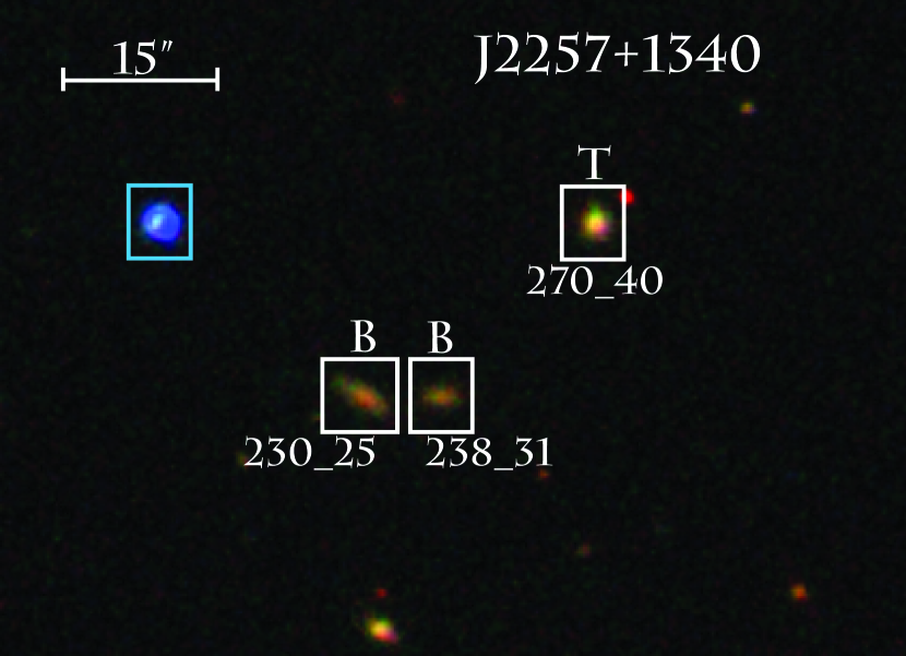
Figure 1.— A three-color (g = blue; r = green; i = red) image of the field J2257+1340. The target (“T”) and bonus (“B”) galaxies are marked and labeled by their identifiers.

In total, we obtained longslit, optical spectra for each of the 38 target galaxies and 29 bonus galaxies over the course of six different observing runs at two telescopes, Keck I and Magellan II Clay. On the Keck I telescope, we used the Low-Resolution Imaging Spectrometer (LRIS), while on the Clay telescope, we used the moderate-resolution Magellan Echellete (MagE) spectrometer. Both instruments provide full coverage of the optical spectrum between approximately 3100 Å  and 9000 Å. Table 1 summarizes the observing runs. Below, we provide details about the observations made with each instrument.

Run	Instrument	Grating(s)	$\lambda_{cen}$ Blue, Red [Å]	Slit	Ngal
(1)	(2)	(3)	(4)
October 2008	LRIS	600/4000, 600/7500	4323, 6905	1.0″	7
March 2009	LRIS	600/4000, 600/7500	4323, 6905	1.0″	7
March 2010	LRIS	600/4000, 600/7500	4323, 7220	1.0″	25
April 2010	LRIS	600/4000, 600/7500	4323, 7056	1.0″	21
March 2011	MagE	175 gr/mm	6200	0.7″	6
May 2011	LRIS	600/4000, 600/7500	4353, 7120	1.0″	1

Table 1 Summary of observing runs. For each grating used, we give the central wavelength in column 3. For LRISb, the spectral coverage is fairly constant at $\sim$ 3100 $-$ 5600 Å. On LRISr, the wavelength coverage begins between 5600 $-$ 5800 Å  while the maximum wavelength ranged from 8200 $-$ 8800 Å. For MageE, the spectral coverage is continuous for 3200 $-$ 10000 Å.

2.1. Keck LRIS Data

Over the course of several observing runs (October 2008, March 2010, April 2010, and May 2011) using the Keck I 10-m telescope Low-Resolution Imaging Spectrometer (LRIS; Oke et al. 1995), we obtained spectra of 61 galaxies (35 target galaxies and 26 bonus galaxies) along 35 QSO sightlines. For these LRIS data, we use a 1 ″ slit, the D560 dichroic with the 600/4000 l/mm grism (blue side) and 600/7500 l/mm grating (red side). Binning the data 2 $\times$ 2 on the blue side and 1 $\times$ 2 (spatial $\times$ spectral) on the red side gives dispersions of 1.2 and 2.3 Å per pixel, respectively. Exposure times varied according to galaxy brightness and sky conditions, but were generally sufficient for obtaining signal-to-noise ratios of at least 3 per pixel for strong nebular emission lines in the galaxy spectra. Table 2 provides some of the observational parameters for the LRIS spectra for each galaxy, including the date observed, exposure times, apparent magnitudes, and flux correction factors (discussed below).

The longslit was typically oriented at a PA to include our target galaxy and either the background quasar or an additional galaxy at close impact parameter to the sightline. We use the LRIS Cassegrain Atmospheric Dispersion Compensator (ADC) to minimize light-loss from atmospheric dispersion. Table 2 summarizes the targets and individual exposures.

In addition to the science observations, we acquired a series of calibration images on each night. Spectral flats on the blue side consist of slitless pixel-flats taken during twilight, which represent the intrinsic pixel-to-pixel response variations of the CCD, and twilight flats with 1″ slit, which represent the larger scale illumination variations due to non-uniformities in the width of the slit and vignetting. On the blue side, we use the twilight sky for spectral flats because the dome lamps emit too little UV light. On the red side, we use the dome flats for both the pixel-to-pixel calibration and the illumination correction since these lamps reduce the level of scattered light. In addition to these spectral flats, we also observed a set of arc lamps at the beginning and end of every night for wavelength calibration, and at least one spectrophotometric standard star per night for flux calibration.

The two-dimensional spectral images were reduced with the LowRedux pipeline, developed by J. Hennawi, D. Schlegel, S. Burles, and JXP. The pipeline bias-subtracts each exposure, generates a flat-field frame from the calibration images, and generates a two-dimensional wavelength image (pixel-by-pixel) from the arc lamp exposures. The code automatically identifies sources in the slit, masks these objects, and calculates a global estimate of the sky background from the remaining pixels. In the majority of cases, this sky solution is refined to be localized to each source during extraction. In several cases, however, we found better results from the global solution alone (especially for pairs of objects in close proximity).

The final 1D spectra were optimally extracted from the two-dimensional images, and multiple exposures of a given target were co-added, weighting by the inverse variance. The wavelength solution of these spectra were corrected for instrument flexure through a comparison of the sky spectrum with an archived solution. The wavelengths were then shifted to a vacuum and heliocentric reference frame.

Spectral fluxing was performed in several steps (see also da Silva et al., 2011). An initial estimate for the flux was made using a sensitivity function generated from our observations of spectrophotometric standard stars. We expect that this provides a good estimate for the relative flux within each camera, but it does not properly account for slit-losses.

To bring the spectra to an absolute flux scale, we convolved the LRISb spectrum with the SDSS $g$-band filter response curve and scaled the flux of the blue spectrum to match the reported SDSS-DR7 petrosian magnitude. Similarly, we matched the $i$-band magnitude for our LRISr spectra. The median values of these two flux factors are 1.94 (blue) and 1.77 (red), corresponding to median slit light losses of 48% and 43%. For a small subset of our sample (seven galaxies), these factors are $>5$. Moreover, the scale factors are occasionally discrepant between the blue and the red sides by more than a factor of 2 (six galaxies, four of which fall into the previous subset). The large and/or discrepant flux scale factors are due to a diverse set of factors: spatially extended galaxies (i.e. systems where slit-loss is extreme), very faint galaxies with high photometric errors, at least one case of probable poor slit alignment, galaxies with close neighbors in projection, and cases of poor seeing $>$ 2″. The SDSS magnitudes and corresponding flux scale factors are listed in Table 2.

Lastly, we applied a correction for Galactic extinction, assuming the $E(B-V)$ value from Schlegel et al. (1998) and a Galactic extinction law (Cardelli et al., 1989). The resultant spectra of the target and bonus galaxies are presented in Figures 2 and  3.

2.2. Magellan MagE Data

In March 2011, three remaining target galaxies and several additional bonus galaxies were observed with the Magellan Echellette (MagE) spectrograph on the Magellan Clay telescope at Las Campanas Observatory (Marshall et al., 2008). MagE provides moderate resolution spectral coverage between 3200 Å and 10000 Å. These data were acquired with a 0.7″  slit and binned 1 $\times$ 1, giving dispersions of 0.3 Å  per pixel at [OII] $\lambda\lambda$ 3727, and 0.5 Å  per pixel at H$\alpha$. The average emission-line FWHM is 55 km s^-1 for these data. Exposure times varied between 600 and 1200 seconds, depending on the target galaxy apparent magnitude. Table 3 provides some of the observational parameters for the MagE spectra for each galaxy, including the date observed, exposure times, apparent magnitudes, and flux correction factors.

The MagE spectra were reduced using the MASE pipeline developed by Bochanski, Simcoe, and Hennawi, which is an adaptation of the MIKE/HIRES echelle extraction codes. 1D spectra are optimally extracted from the 2D reduced images. Several spectrophotometric standard stars taken at a variety of airmasses were used to initially flux-calibrate the data. As with the LRIS data, we account for slit-losses by scaling the spectra to match SDSS photometry. Because there is no dichroic in the MagE data, we correct these spectra with the SDSS $r$-band photometry. Once we scale the spectra by the appropriate flux factor, we confirm that the resultant colors in the SDSS bands match to within 0.2 magnitudes and conclude that the $r$-band normalization is approximately correct for $u$ and $g$ bands as well.

3. Analysis

3.1. Redshift Determination

It is of primary scientific interest to our program, which examines the gas in galactic halos, to establish a precise redshift for each target galaxy. One can then search the spectra of background quasars for any coincident absorption. All of our target galaxies exhibit significant absorption lines (e.g. Ca H+K) and/or emission lines (e.g. H$\beta$) which provide a precise redshift measurement for stars and the ISM (Figure 2 and 3). Instead of analyzing these spectral features individually, we employed a modified version of the SDSS algorithm zfind that is bundled within the IDLUTILS package. In brief, the code models the input LRIS spectrum using a set of archived Principle Components Analysis (PCA) eignevectors derived from galaxies observed in the SDSS survey. We also include a model of the instrumental spectral resolution, allowing and solving for internal dispersion within the galaxy. The code calculates the $\chi^{2}$ in steps of redshift space, reports the minimum value, and provides an estimate of the redshift uncertainty.

For the Keck/LRIS observations, we performed this analysis on the red and blue sides of the spectra separately. In two cases of very faint galaxies at low redshift, only the H$\alpha$ emission line is present in the LRISr spectrum and $zfind$ fails on the red side. In these two cases we manually entered the red-side redshift to be equal to that of the blue side, which was based on [OII], H$\beta$ and [OIII]. As the statistical uncertainties reported by zfind are generally $<$ 5 km s^-1, the precision of our redshift measurements is limited by systematic uncertainty. The RMS of the wavelength solution and the flexure correction are the two primary sources of error. The two independent redshift determinations on the red and blue sides offer some insight into its magnitude.

The top panel of Figure 4 compares the resultant LRISb and LRISr zfind redshifts in velocity space. This plot shows that the redshifts derived from the blue camera tend to be systematically higher than those derived from the red camera by nearly 10 km s^-1. Such an offset may result from: (1) The difference in the instrumental flexure correction for the blue and red cameras, and (2) the use of the unresolved [OII] $\lambda$$\lambda$ 3727 doublet in the redshift determination of the blue camera. The [OII] emission line is often the strongest spectral feature in that spectrum. Since the flexure correction is done with night-sky lines, the blue side is subject to higher uncertainty owing to there being far fewer sky lines below 5000 Å. Taking into account both of these effects, we are inclined to trust the redshifts from the red side over the blue. The resultant redshifts from LRISr are listed in the third column of Table 5. We estimate the overall uncertainty of the redshifts given in the table by the standard deviation of the redshift differences between the red and blue sides seen in Figure 4. Thus, we adopt a conservative 30 km s^-1 systematic uncertainty in our final redshift measurements. This uncertainty is primarily due to wavelength calibration error (a combination of RMS in the arc-line analysis and instrument flexure).

To determine the precise redshifts of the galaxies observed with Magellan MagE, we use the same SDSS zfind algorithm for the entire spectrum. Thus, the redshifts we report in Table 5 for the MagE galaxies were made using the entire spectrum. Because the spectral resolution of MagE is higher than that of LRIS (the [OII] $\lambda$$\lambda$ 3727 doublet is resolved in these spectra), the systematic uncertainty in the MagE redshifts is lower than that of the LRIS redshifts. We estimate the uncertainty of these redshifts to be 5 km s^-1, based on the RMS of the wavelength calibration.

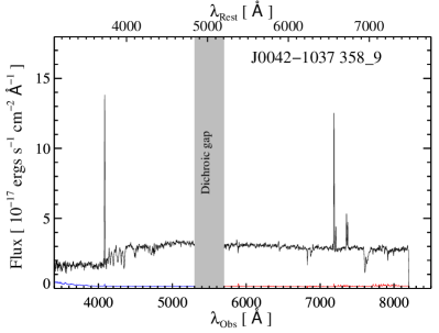
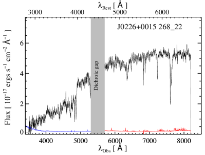
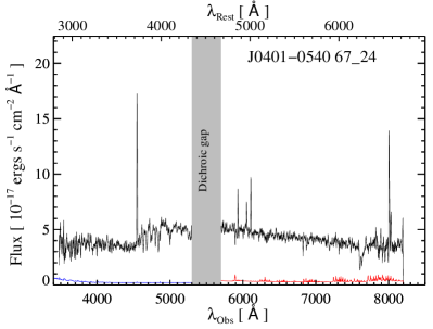
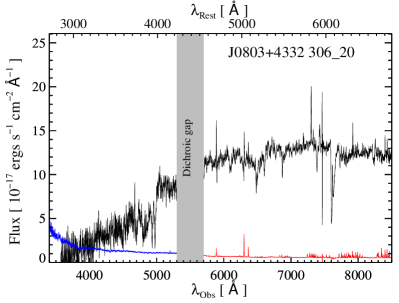
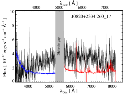
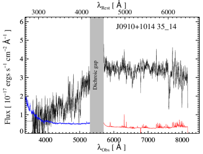
Figure 2.— The 1D reduced, flux-calibrated spectra for selected target galaxies. All spectra will be available in the online, published version.We represent the dichroic with a shaded area near the observed wavelength 5000 Å.

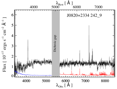
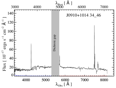
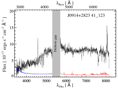
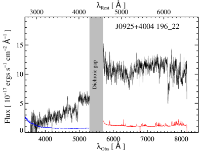
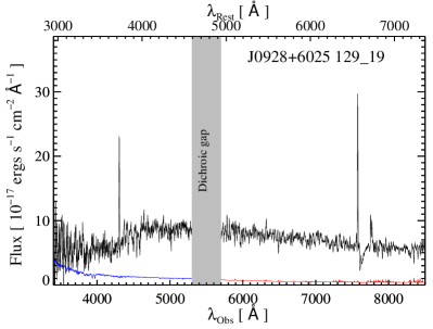
Figure 3.— The 1D reduced, flux-calibrated spectra for selected bonus galaxies. All spectra will be available in the online, published version. We represent the dichroic with a shaded area near the observed wavelength 5000 Å.

We made one final check on our redshift estimates following Rubin et al. 2011, who note modest, but non-negligible, offsets between emission lines and stellar absorption features in spectra of $z\sim 0.5$ galaxies. The bottom panel of Figure 4 compares the redshift measurements from zfind made using the entire LRISr spectrum (z_spec) against a similar analysis but with galaxy emission-line features masked out (z_abs). There is generally good agreement between z_spec and z_abs, with no significant systematic offset between the two measurements. Furthermore, the standard deviation of this distribution (6 km s^-1) falls well-within the adopted 30 km s^-1 systematic redshift uncertainties. Therefore, we do not consider this a significant concern for our analysis.

Figure 4.— Top: velocity difference between blue and red-side spectral redshifts. Bottom: Velocity difference between redshifts measured using all spectral features, and redshifts measured after masking out emission lines. The red-side spectral redshift using the full spectrum is on the x-axes of both plots. Dashed-dotted lines mark the standard deviation (top and bottom lines) and mean (middle line) of the distribution of these differences.

In Figure 5 we plot the galaxy SDSS photometric redshifts (z_phot) versus their spectroscopic redshifts (z_spec). For reference, the values of z_phot that we use here are part of the “Photoz2” online catalog, and called “photozd1.” These redshifts and their errors are calculated using SDSS galaxy magnitudes and a Neural Network method (Oyaizu et al., 2008). The gray shaded region of this plot highlights the original COS-Halos survey redshift selection criterion, while the hashed area is shown to mark the region of spectroscopic redshift parameter space that ultimately falls outside of the pre-selected range. In order the assess the accuracy of the z_phot, we calculate $\chi^{2}$ assuming that the relation between z_phot and z_spec should be a one-to-one linear correlation. We find that $\chi^{2}$ is quite large in this case (n_dof = 64; excludes the two galaxies in the sample not identified by SDSS), with a value of $\sim$115, and has an associated probability of $\sim$0.1%. If we exclude those points that fall within the hashed area of this plot, $\chi^{2}$ is lowered considerably to $\sim$55 (n_dof = 53), corresponding to a probability of $\sim$40%. Thus, the large $\chi^{2}$ for the full sample is driven by a handful of “catastrophic failures.” On this plot, we also show error-weighted linear-least-squares fits to the data using the full sample (dotted line) and the constrained sample in which 0.11 $<$ z_spec $<$ 0.38 (dashed line). The fits to the two samples are: z_fit = (0.05 $\pm$ 0.01) + (0.77 $\pm$ 0.07)$\times$z_spec, with a $\chi^{2}$ of 99.25 (P = 0.24%), and z_fit (0.11 $<$ z_spec $<$ 0.38) = ($-$0.005 $\pm$ 0.02) + (1.07 $\pm$ 0.09)$\times$z_spec , with a $\chi^{2}$ of 49.6 (P = 56.8%).

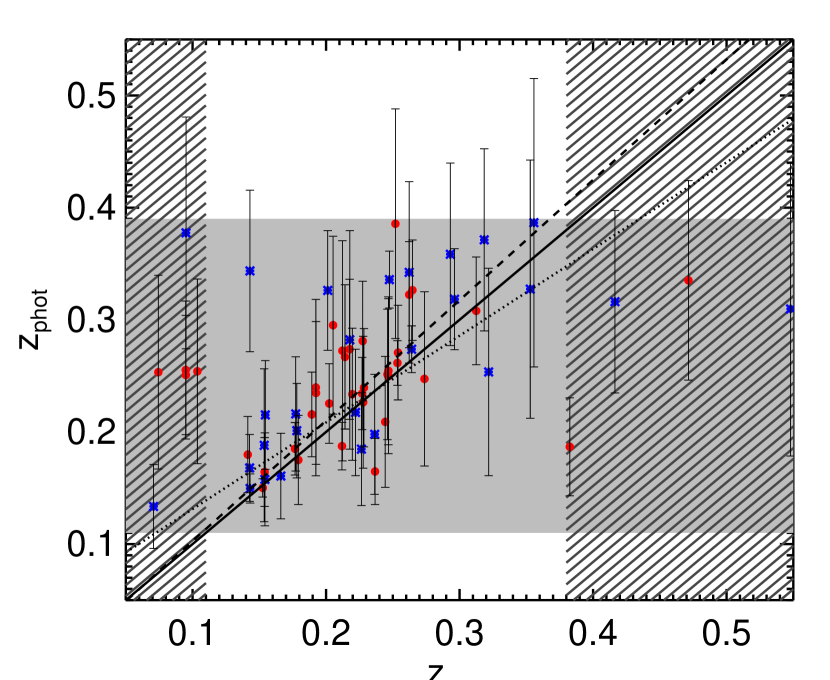
Figure 5.— SDSS photometric redshifts versus LRIS and MAGE spectroscopic redshifts. We show target galaxies as red filled circles and bonus galaxies as blue asterisks. The shaded area of the plot highlights the original sample selection criteria described in Tumlinson et al. 2011, while the hashed area of the plot highlights those objects with spectroscopic redshifts that ultimately fall outside the selected redshift range. The one-to-one line is shown as a solid line. The dotted line represents a fit to all the data, while the dashed line represents a fit to the data in the range 0.11 $<$ z_spec $<$ 0.38.

3.2. K-corrections: Stellar Masses and Absolute Magnitudes

To obtain an estimate of the current stellar mass and absolute magnitudes of each galaxy, we used version 4_2 of Michael Blanton’s IDL package $kcorrect$ (Blanton & Roweis, 2007), the SDSS DR7 galactic reddening corrected, asinh $ugriz$ magnitudes, and the $zfind$ spectral redshifts. Specifically, we use the routine $sdss$_$kcorrect$ to obtain a suite of distance-dependent galaxy properties for every galaxy in our sample. Two exceptions are the bonus galaxy J1009+0713: 86_4 and target galaxy J1157-0022: 230_7 which lie at very close impact parameters to the QSO and are not identified as separate galaxies in the SDSS catalogs. The stellar masses and absolute magnitudes that are output by $sdss$_$kcorrect$ contain a factor of $5\log h$, with the unitless $h=1$. The masses and absolute magnitudes we adopt throughout this work have been corrected assuming the 5-year WMAP cosmology with a $h=0.72$ (Dunkley et al., 2009).

For red galaxies that are not detected by SDSS in the $u$-band, we put realistic flux-based limits on the absolute $u$-band magnitude rather than employ the output k-corrected asinh absolute magnitude (which may even be based on a negative flux). The procedure for determining these limits is as follows: (1) we use the routine $k\_lups2maggies$ to convert SDSS luptitudes (asinh magnitudes) to maggies (a flux-like quantity), (2) we then input the maggies and their inverse variance into $sdss\_kcorrect$ to obtain absolute magnitudes (M) and their inverse variances (M_ivar), (3) we determine the corresponding absolute maggie (F_maggie) and its inverse variance (F_ivar), taking F_maggie = 10^-0.4M and F_ivar = M_ivar / (0.4 $\times$ ln10 $\times$ F_maggie)², (4) We determine an absolute magnitude limit (M_lim) in the $u$-band for each individual galaxy such that M_lim = -2.5 $\times$ log₁₀ (2 $\times$ (1/F_ivar)^1/2). If a detection of a galaxy in the $u$-band is less than 3$\sigma$, we adopt a 2$\sigma$ magnitude limit and report a lower limit to the $u-r$ color.

The middle-left panel of Figure 7 shows the distribution in log space of stellar masses for the full sample of foreground galaxy masses (light shade) and for only the target galaxies (dark shade). These stellar masses are also listed in Table 5. The median log $M_{*}$ is 10.31, in a distribution that ranges from $\sim$ 8.8 $-$ 11.3. The mass distribution of SDSS galaxies (based on photometric redshifts and stellar absorption line indices) shows a bimodal distribution with a break near 10.4, above which there is an increasing fraction of older-population elliptical galaxies (Kauffmann et al., 2003). Our sample brackets this break but contains very few systems with $M_{*}\ll 10^{10}M_{\odot}$. This bias results from our sample selection criteria that were meant to isolate L* galaxies. We selected galaxies from SDSS that had apparent magnitudes sufficiently bright to provide a precise photometric redshift $z_{\rm phot}$ and also yielded $z_{\rm phot}\approx 0.2$ to enable a search for O vi absorption.

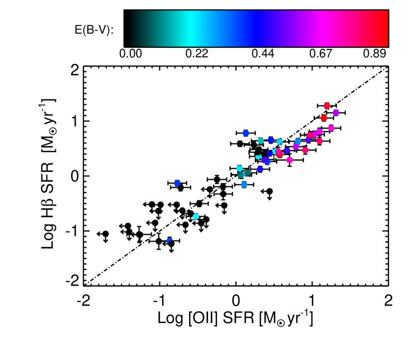
Figure 6.— [OII] vs H$\beta$ SFR, where the color represents the magnitude of the E(B-V) Balmer correction derived from the observed H$\alpha$ to H$\beta$ ratio. Black points indicate that no Balmer correction was made because we did not detect H$\alpha$ or H$\gamma$. Those galaxies with the highest SFRs also tend to have the highest Balmer corrections. Upper limits to the SFRs are shown with left-facing and downward-facing arrows. The galaxies at high SFR tend to deviate from the one-to-one line because of a probable overestimation of the reddening at [OII].

3.3. Spectral Measurements

A galaxy spectrum dominated by active star formation will exhibit emission lines that indicate its level of metal-enrichment and current star formation rate (SFR). Here we describe the initial line measurements and corrections made to the emission-line galaxies in our sample. For non-emission-line galaxies in which the spectrum is dominated by stellar continuum and absorption, we describe the measurements that allow us to obtain upper limits on the SFR.

We developed an IDL-based graphical user interface program (bundled within XIDL) named $gal\_fit\_emiss$, to fit spectral features with Gaussian profiles and/or boxcar fits that give integrated line fluxes and associated photon noise errors. We compute the line FWHMs using $galx\_fit\_emiss$, where the line Gaussian FWHM (km/s) = c $\times$ FWHM (Å) / $\lambda_{line}$ (Å). The average line FWHMs are 280 (blue) and 200 (red) km/s. These values are dominated by the spectral resolution as the lines are unresolved. For Balmer emission-lines, we minimize contamination from underlying stellar absorption by fitting the continuum in the trough of detectable absorption. The overall effect on the line flux of the Balmer absorption ranges from 10% to 60% for the H$\beta$ emission line (when absorption is apparent).

We apply a correction for interstellar reddening to all line measurements from the observed H$\gamma$ to H$\beta$ and H$\alpha$ to H$\beta$ ratios for case B recombination where H$\gamma$/H$\beta$ = 0.459 and H$\alpha$/H$\beta$ = 2.86 at an effective temperature of 10,000 K and electron density of 100 cm^-3 (Hummer & Storey, 1987). We use a reddening function normalized at H$\beta$ from the Galactic reddening law of Cardelli et al. (1989) assuming R_v = A_v/E(B$-$V) = 3.1. We do not apply a correction for internal interstellar reddening when we cannot measure the line fluxes of at least 2 Balmer emission lines. We tabulate the line fluxes and the E(B-V)_Balmer in Tables 4 and 5.

The error in the final reddening-corrected line flux measurement is due to three primary factors: (1) the photon noise, which is the least significant source of error, (2) the error in the Balmer correction, which is based on the uncertainty in the flux ratio used to calculate the Balmer correction and the intrinsic error ($\approx 10\%$) in the assumed constants (0.459, 2.86), and (3) the error in the slit correction flux scale factor, assumed to be 10%. The dominant error term is the Balmer correction, especially for galaxies that turn out to be very dusty. The average reddening is E(B-V) = 0.3 for the galaxies in our sample where we measured the Balmer decrement.

3.4. Star Formation Rates

Once we correct the galaxy spectrum for the Balmer decrement, we calculate a current SFR using the Balmer emission lines H$\alpha$ and H$\beta$ and the [OII] $\lambda$$\lambda$ 3727 doublet. For the former, we use the calibration of Kennicutt (1998) where SFR [M_⊙ yr^-1] $=$ 7.9 $\times$ 10^-42 L_Hα [ergs s^-1]. Balmer emission lines are the most straightforward of emission-line SFR indicators because their luminosity directly traces the ionizing stellar populations. The Kennicutt (1998) H$\alpha$ SFR calibration is derived from stellar population synthesis models that assume a Salpeter IMF (Salpeter, 1955) and solar metallicity. When H$\alpha$ is not observed in a spectrum, we use the same Kennicutt (1998) SFR calibration divided by a factor of 2.86 for the H$\beta$ emission line. At an effective temperature of 10,000 K and electron density of 100 cm^-3 for Case B recombination, this factor of 2.86 is the intrinsic ratio of H$\alpha$/H$\beta$ (Hummer & Storey, 1987). Thus, the SFRs derived from H$\alpha$ and H$\beta$ are identical when we calculate a dust correction that gives H$\alpha$/H$\beta$ = 2.86.

Additionally, we tabulate [OII] SFRs using equation 4 of Kewley et al. (2004), where SFR [M_⊙ yr^-1] $=$ 6.58 $\times$ 10^-42 L_[OII] [ergs s^-1]. [OII] SFR indicators are more complicated than Balmer emission line indicators because [OII] is affected by reddening, ionization properties, stellar absorption, and metallicity. Ideally, we would adopt the [OII] SFR indicator that contains a correction for oxygen abundance, but not all of our galaxies have emission lines or wavelength coverage that permit a metallicity estimate. Figure 6 compares [OII] and Balmer SFRs, and shows that they correlate well, but that there is a large scatter of $\sim$ 0.3 dex. This plot also shows the internal reddening correction in $E(B-V)$ for every galaxy in which we can measure it. The galaxies that deviate from the one-to-one line at high SFR are likely to suffer from an overestimation of the reddening at [OII]. The corrections at H$\alpha$ are small ($\sim$3%) such that uncertainties in $E(B-V)$ and the extinction curve do not have a significant impact on the Balmer-derived SFRs.

When a galaxy’s spectrum contains no emission lines, we measure an upper limit to the SFR by measuring the boxcar noise at the positions of [OII], H$\beta$ and H$\alpha$. We use 3$\sigma$ line flux limits as our SFR upper limits in these cases, approximately 1/3 of our sample. We adopt conservative 3$\sigma$ limits to the SFRs since in these galaxies we are unable to make a correction for dust. There is a set of red galaxies where [OII] emission is present yet we have a strict limit on Balmer emission. This is a somewhat common occurance in galaxy surveys and has been attributed to AGN activity (e.g. Konidaris et al., 2007). In these cases, we measure the [OII] line-flue but attribute an upper limit to the inferred SFR. These are generally much higher than the Balmer SFR upper limit for the same galaxies. In Table 5 we list SFRs, their errors, and mark the upper limits.

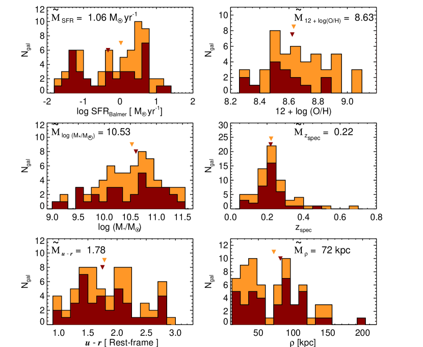
Figure 7.— Distribution of several key derived galaxy properties for the entire sample of galaxies (light shade) and for target galaxies (dark shade). The median of each full distribution is marked with a light yellow, filled triangle, and labeled. The medians of the target galaxy distributions are marked with a corresponding dark red filled triangle.

3.5. Metallicity Determination

When the necessary emission lines are present, we use two separate strong-line methods of determining the oxygen abundances for our foreground galaxies : the R₂₃ = ([OII] $\lambda$3727 + [OIII] $\lambda\lambda$4959, 5007) / H$\beta$ (Pagel et al., 1979) calibration of McGaugh (1991; henceforth M91), and the N2 index, the [NII]$\lambda$6583/H$\alpha$ ratio, based on the calibration of Pettini and Pagel (2004; henceforth PP04). Below, we describe each method in detail and discuss the systematic uncertainties.

The M91 R23 oxygen abundance has a relative error of $\sim$0.15 dex over a wide range of abundances, but exhibits a well-known degeneracy, with a turn-over in the relation at Z $\sim$ 0.3 Z_⊙ (12$+$log(O/H) $\sim$ 8.35). The oxygen abundance is given by the following two analytic expressions for lower and upper branches (Kobulnicky et al., 1999):

$$12+\log({\rm O/H})_{lower}= 12-4.944+0.767x+0.602{x}^{2}$$ (1)

$$-y(0.29+0.332x-0.331{x}^{2}),$$

$$12+\log({\rm O/H})_{upper} =12-2.939-0.2x-0.237x^{2}$$ (2)

$$-0.305x^{3}-0.283x^{4}-y(0.0047$$

$$-0.0221x-0.102x^{2}-0.0817x^{3}$$

$$-0.00717x^{4}),$$

where x $=$ log R₂₃ and y $=$ log ([OIII] $\lambda$ 4959 + [OIII] $\lambda$ 5007)/ [OII] $\lambda$ $\lambda$ 3727.

The most robust way to place a galaxy on the upper or lower branch of the R23 relation is to use the [NII] $\lambda$6583 to [OII] $\lambda$$\lambda$3727 ratio. When log [NII]/[OII] $<$ $-$1.0, it lies on the lower metallicity branch of the R23 relation (M91), and correspondingly, when log [NII]/[OII] $>$ $-$1.0, an upper-branch metallicity results (Kewley & Ellison, 2008). The line flux ratio [NII]/H$\alpha$ (the N2 index) provides an alternative method. If log N2 $<$ -1.3 ([NII]/H$\alpha$ $<$ 0.05) there is a high degree of certainty that the oxygen abundance is on the lower branch of the R23 relation. Whereas if log N2 $>-1.1$ ([NII]/H$\alpha$ $>$ 0.08) the oxygen abundance is on the upper branch. Between $-1.1$ and $-1.3$, the N2 index does not accurately discriminate between upper and lower branches of R23 because the oxygen abundance is likely to be very close to the turnover at 12 $+$ log (O/H) $=$ 8.3.

The benefit to using the N2 index over log [NII]/[OII] is that the former involves two lines in close wavelength proximity ($\lambda$ [NII] = 6583 Å; H$\alpha$ = 6563 Å) such that the flux calibration and reddening correction have little to no impact on the resultant line ratio. The N2 index itself is sensitive to the metallicity to within 0.35 dex accuracy at a 95% confidence level up to 12 + Log(O/H) = 8.8 (Pettini and Pagel 2004, henceforth PP04). We use the following expression from PP04 to calculate the oxygen abundance from the N2 index:

$$12+log({\rm O/H})=9.37+2.03\times N2+1.26\times N2^{2}+0.32\times N2^{3},$$ (3)

where N2 $=$ log ([NII] $\lambda$6584/H$\alpha$). The PP04 calibration is valid for $-2.5<N2<-0.3$, or 7.20 $<$ 12$+$ log (O/H) $<$ 8.95. The benefits of this strong-line abundance indicator are that it is monotonic with (O/H) and it does not require precise flux calibration or a reddening correction due to the proximity in wavelength of [NII] $\lambda$6583 and H$\alpha$. The primary drawback is the large uncertainty in the calibration (0.35 dex), and the limited range over which it is useful. We tabulate PP04 oxygen abundances in Table 5, and note that there are several galaxies with N2 indices $>-0.3$ which give values of 12$+$ log (O/H) outside the valid range. We show these values of the PP04 abundance as lower limits where 12 $+$ log (O/H) $>$ 8.95.

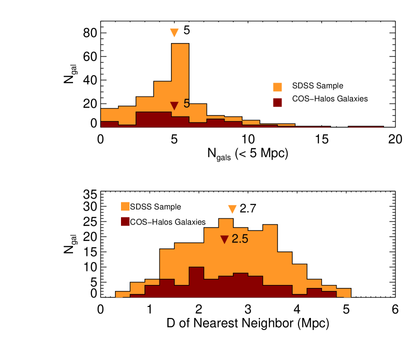
Figure 8.— Two histograms that show the number of galaxies within 5 Mpc of a given COS-halo galaxy (top) and the distance to the nearest neighboring galaxy in Mpc (bottom). In both plots the median values are marked for a randomly selected sample of SDSS galaxies in the same redshift range (light shade) and the COS-Halos galaxies (dark shade).

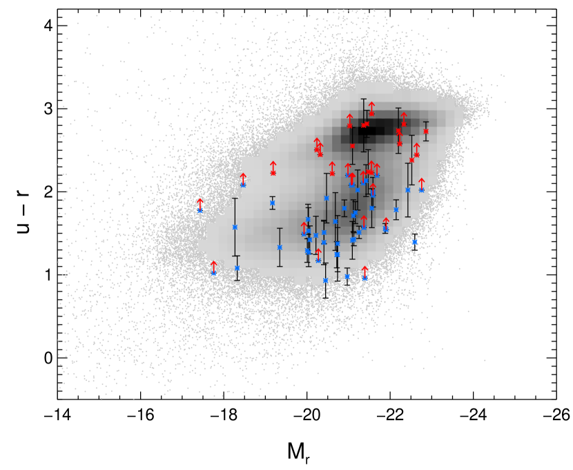
Figure 9.— A color-magnitude plot for the COS-Halos galaxies, where blue galaxies ($u-r$ $<$ 2.2) are plotted as blue asterisks and red galaxies ($u-r$ $\geq$ 2.2) are shown as red asterisks. Error bars for the galaxy k-corrected colors are shown unless a red, upward-facing arrow indicates a u$-$r lower limit as discussed in Section 3.2. The shaded histogram is shown for local SDSS galaxies, and grey points are plotted when the number of SDSS galaxies is less than 100.

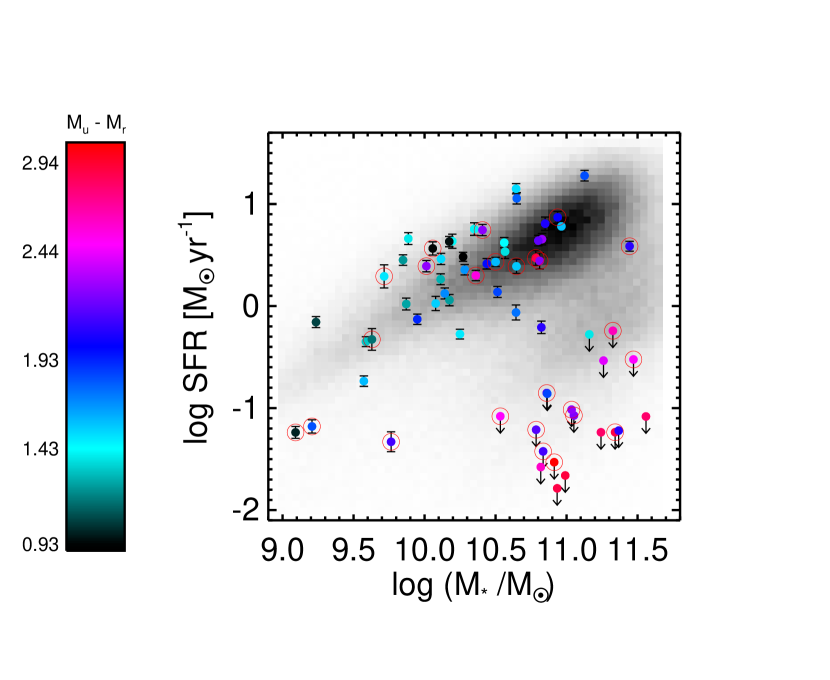
Figure 10.— Log SFR measured from either H$\alpha$ or H$\beta$ emission versus Log M_∗. Points in this figure are color-coded for galaxy u$-$r color, where red open circles indicate a u$-$r lower limit as discussed in 3.2. The number density distribution of $\sim$10⁵ SDSS star-forming galaxies is shown in grayscale, for reference. The SFRs and stellar masses come from the MPA Value Added Catalogs, and are based on the comprehensive studies by Brinchmann et al. (2004), for the SFR (median values are corrected to a Salpeter IMF, to match the calibration we use in this study), and by (Kauffmann et al., 2003), for the stellar masses.

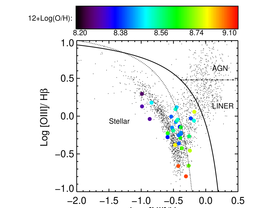
Figure 11.— A BPT diagram (Baldwin et al., 1981) showing the nominal flux ratios (log [OIII] $\lambda$5007/ H$\beta$ vs. log [NII] $\lambda$6584 / H$\alpha$) for a subset (32 of 67) of the entire sample of galaxies having available line measurements. The colors of the points correspond to galaxy oxygen abundances derived from the McGaugh 1991 calibration of the R23 relation. The black dots correspond to a random selection of galaxies from SDSS DR7, and roughly demarcate the full range of flux ratios observed for local galaxies. The two curves are two different calibrations (solid: Kewley et al. 2001; dashed: Kauffmann et al. 2003) that attempt to separate emission from ionized nebulae (star formation) from emission due to other processes (AGN, LINERs). The horizontal line separates AGN from LINERs. (Veilleux & Osterbrock, 1987)

In the cases for which we are unable to measure a Balmer decrement (e.g. H$\beta$ falls in the dichroic), and the few cases for which we do not trust the absolute flux calibration for red-blue side matching (large uncertainty in SDSS apparent magnitudes), we prefer the N2 index to log [NII]/[OII] for breaking the degeneracy of the R23 relation. Furthermore, when H$\alpha$ and [NII] lie outside the observed wavelength range for the galaxy, we cannot properly break the degeneracy of the R23 relation (7 emission-line galaxies). Fortunately, there is a well-known global relation between galaxy mass and metallicity, the mass-metallcity relation (Skillman et al., 1989; Tremonti et al., 2004), that enables us to make an informed guess as to R23 branch. The majority (66 of 68) of our galaxies have stellar masses $>$ 10${}^{9}M_{\odot}$, making it more likely that they are on the upper branch of the R23 relation than the lower branch. In Section 4, we further discuss the mass-metallicity relation of our sample of foreground galaxies.

McGaugh (1991) reports several different values of the systematic error associated with this strong-line calibration depending on the resultant oxygen abundance: 0.1 dex for the upper branch, 0.05 dex for the lower branch, and 0.20 dex within 0.1 dex of the R23 turnover. Additional, unaccounted for sources of error arise from HII region age-effects (M91 is calibrated for zero-age HII regions) and geometrical effects (Stasińska & Leitherer, 1996; Ercolano et al., 2007). The overall impact of these effects increases the systematic error in this method to 0.1 $-$ 0.3 dex, on average, regardless of branch, and in the “worst-case” scenario. We adopt $\pm$0.15 dex as an average systematic error in our abundance measurements, unless a value is within 0.1 dex of the turnover, where it is then estimated to be $\pm$0.2 dex. Neither the M91 nor PP04 calibration indicates an oxygen abundance on an absolute scale better than to a factor of $\sim$0.3 dex, and there are well-known systematic offsets between the two methods (Kewley & Ellison, 2008).

4. Results: Global Properties of the Galaxies

As described in Section 1, the data and analysis presented in the proceeding sections are associated with a galaxy sample selected from the SDSS for a targeted study of gas in the halos of $L\approx L^{*}$ galaxies at $z\sim 0.2$. This blind survey was designed to sample galaxies with a range of stellar mass, star-formation rate, and color. In this final section, we describe the distribution of galaxy characteristics for the sample, provide global context for their properties, and highlight differences (if any) from the general low-$z$ population.

The properties of the galaxies in our sample are summarized by the histograms in Figure 7, where the full galaxy sample (targets + bonus) is shown by the light-yellow shade histograms and the target galaxies are shown by the dark-orange shade histograms. The distribution of SFRs shows a bimodality, separated at $\sim$0.1 M_⊙ yr^-1. The majority of SFRs below this value are upper limits, i.e. the lower of the two three-sigma Balmer SFR limits. This apparent bimodality, then, is more a reflection of the sensitivity limit of our spectral data than it is a sign of any physical bimodality of SFRs in our sample.

As we discussed in Section 3.2, our original sample criteria select against lower-mass galaxies compared to the universal distribution. These same selection effects also result in a metallicity distribution that is lacking in the lowest-metallicity galaxies (i.e. dwarfs), as expected from the mass-metallciity relation. As expected and desired, our selection of galaxies to have $zphot$ between 0.11 and 0.4 leads to a distribution in the spectroscopic redshifts that is clustered around a median value of $\sim$ 0.2. As seen in Figure 5, the SDSS-based $zphot$ is occasionally highly skewed, and there are several galaxies in our sample that we found to have redshifts $<$ 0.11 or $>$ z_QSO, making their OVI lines unobservable with the COS spectrograph. The median impact parameter for our sample is 118 kpc in the galaxy rest frame. Finally, k-corrected $u-r$ colors show a distribution between 1 and 3, with a median of 1.8 magnitudes.

To examine the environments of the COS-Halos galaxies, we first searched the maxBCG galaxy cluster catalog (Koester et al., 2007) for any likely matches. The following galaxies turn out to lie in or near a maxBCG galaxy cluster: J0928+6025: 110_35 (7.95 Mpc from cluster center), 129_19 (7.38 Mpc from cluster center), and 187_15 (9.08 Mpc from cluster center)); J1157-0022: 359_16 (12.35 Mpc from cluster center); and J1514+3620: 287_14 (19.3 Mpc from the cluster center). Furthermore, we compare the neighborhood of the COS-Halos galaxies to that of a random selection of $\sim$500 SDSS galaxies of similar luminosities and in the same redshift range. Figure 8 shows the results of this comparison. The distances between galaxies are comoving distances computed such that D_tot = $\sqrt{(}D_{CM,z1}^{2}+D_{CM,z2}^{2}-2D_{CM,z1}D_{CM,z2}cos\theta)$. In this equation, D_tot is the comoving distance from one galaxy at redshift z1 to another galaxy at redshift z2 with a projected angular separation, $\theta$, in radians. Figure 8 shows the number of galaxies within 5 Mpc of a given galaxy and the distance to the nearest neighboring galaxy in Mpc. When environment is assessed in this manner, we find essentially no differences between our sample and the control SDSS sample.

We show a color-magnitude diagram for the COS-Halos galaxies and numerous SDSS galaxies in Figure 9. The k-corrected colors and absolute magnitudes of the SDSS galaxies come from the NYU Value-Added Galaxy Catalog (Blanton et al., 2005), and are further corrected to account for our adopted cosmology (i.e. a factor of 5$log$h). Although the COS-Halos galaxies fall within the main locus of SDSS galaxies, blue galaxies are somewhat over-represented in our target galaxy sample. One goal of the COS-Halos project is to examine the relation of galaxy star-forming properties to halo properties, and we originally selected a blue-biased galaxy sample to probe the full range of galaxy star-forming properties.

A galaxy’s SFR is anti-correlated with its stellar mass, a trend we reproduce in Figure 10. Points in this figure are color-coded for galaxy u$-$r color and show that the redder galaxies with SFR upper limits in this sample are on average more massive than bluer SF galaxies. The red open circles indicate a u$-$r lower limit as discussed in 3.2. The number density distribution of $\sim$10⁵ SDSS star-forming galaxies is shown in grayscale, for reference. The SFRs and stellar masses come from the MPA Value Added Catalogs , and are based on the comprehensive studies by Brinchmann et al. (2004), for the SFR (median values are corrected to a Salpeter IMF, to match the calibration we use in this study), and by Kauffmann et al. (2003), for the stellar masses. In this parameter space, the COS-Halos galaxies appear to trace the bimodal distribution of SDSS galaxies such that red, massive galaxies with very low SFRs separate cleanly from bluer galaxies with higher SFRs.

We plot the log [OIII] $\lambda$5007/ H$\beta$ vs. log [NII] $\lambda$6584 / H$\alpha$ line flux ratios in Figure 11, in a BPT diagram (Baldwin et al., 1981) useful for separating emission due to ionized nebulae (star formation) from emission due to other processes (AGN, LINERs). The star-forming sequence is delineated by two curves: the dotted line (Kauffmann et al., 2003) separates purely star-forming galaxies (left) from other types of active galaxies (right), and the solid line (Kewley et al., 2001) demarcates galaxies that have emission from combined sources, including star formation, from pure AGN. Every emission-line galaxy in our sample is associated with at least some star formation, with 5/30 exhibiting combined emission. For these 5 galaxies, metallicities and star formation rates have more complicated interpretations since the strength of emission lines will not directly correlate with either quantity in an AGN spectrum. These galaxies are classified as “combined SF/AGN” in the galaxy type column of Table 5.

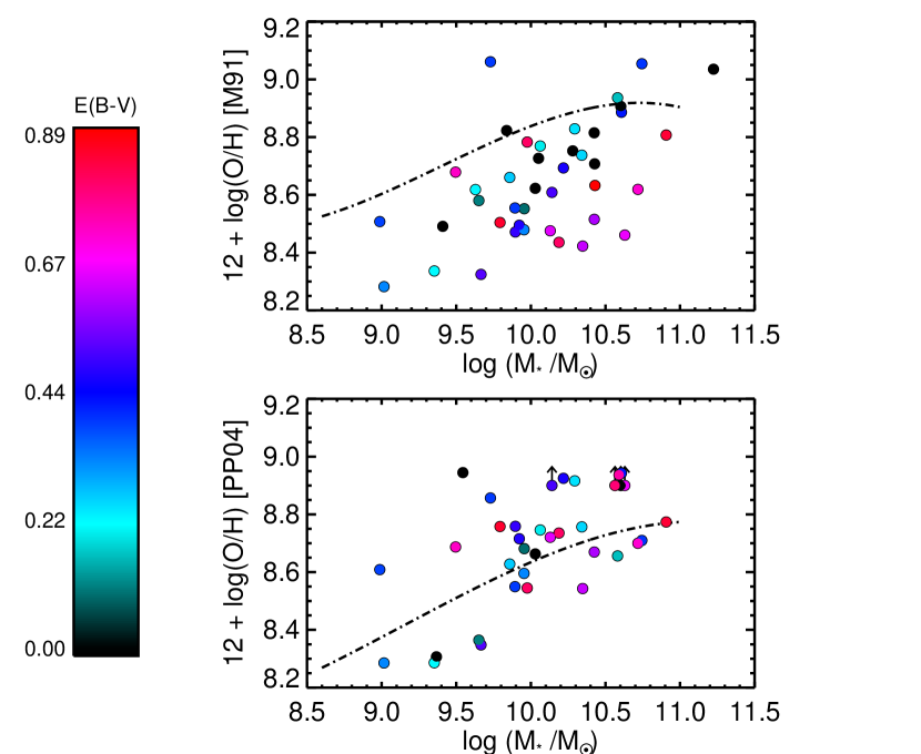
Figure 12.— The mass-metallicity relation for a subset of galaxies in our sample having metallicity estimates based on the M91 calibration of the R23 relation (top panel) and based on the PP04 calibration of the N2 index (lower panel). Stellar masses are determined from Michael Blanton’s $k-correct$ (Blanton & Roweis, 2007), and corrected for a factor of $5logh$ where $h=0.72$ in our adopted cosmology. The dashed-dotted curves come from fits to SDSS data from Kewley & Ellison (2008), for both the M91 (top) and PP04 (bottom) calibrations.

In Figure 12 we show the mass-metallicity relation for the emission line galaxies in our sample using both M91 and PP04 oxygen abundance calibrations. Generally, we reproduce the well-known trend that more massive galaxies tend to contain more metals. Comparing our relations with the calibration-dependent fits to SDSS data of Kewley & Ellison (2008), we see that our M91 mass-metallicity relation is discrepant from the fit to SDSS data of Kewley & Ellison (2008), while the PP04 fit is better. It is unclear what is causing this discrepancy in the M91 calibration mass-metallicity relation. The offset is opposite what we would expect if reddening corrections are systematically underestimated (due to not being able to make any reddening corrections for several galaxies because of lacking necessary emission lines). However, even if reddening is overestimated for many of the galaxies, its effect would be, at most, on the level of 0.1 dex. Furthermore, we do not find a significant offset between M91 and PP04 oxygen abundances for our sample of galaxies, as do Kewley & Ellison (2008). The typical scatter in the mass-metallicity relation (0.3 dex) is reflected in these plots.

5. Summary

In this paper, we describe the details of the optical observations and spectral analyses done as part of the COS-Halos survey (Tumlinson et al. 2011). The high signal-to-noise optical spectra for 67 galaxies from Keck LRIS and Magellan MagE presented here are essential to the COS-Halos survey that aims to explore the variations of halo gas properties with galaxy properties. We determine and tabulate galaxy spectroscopic redshifts accurate to $\pm$ 30 km s^-1, impact parameters, rest-frame colors, stellar masses, total star formation rates, and gas-phase interstellar medium oxygen abundances.

The COS-Halos target galaxy sample was pre-selected to span redshifts of 0.1 $-$ 0.3, stellar masses log(M_∗/M_⊙) = 9.5 $-$ 11.5, and be located $<$ 160 kpc from a background QSO sightline. These criteria bias the galaxies to have higher than average galaxy masses (and, by extension, higher than average metallicities), and may further select against galaxies with spectra dominated by AGN (see Figure 11). Within the pre-selection criteria, the COS-Halos galaxies are well-sampled with respect to mass and star formation, with 2/3 of the galaxies being dominated by ongoing star-formation. A wide range of SFRs (0.01 $-$ 20 M_⊙ yr ^-1) will allow us to investigate the connection between galaxy bimodality and halo gas. Although three of the COS-Halos target galaxies were found to be part of Galaxy clusters, we do not find that the environments of the galaxies are on average significantly different from those of the general low-redshift, L* galaxy population. Through this analysis, we are able to reproduce well-known correlations between galaxy metallicity and mass, galaxy global SFRs and galaxy mass, and find no significant deviations. In total, the COS-Halos galaxy sample is representative of a normal set of L$\sim$L* galaxies at z$\sim$ 0.2. Subsequent analyses using the COS-Halos survey data will rely on the galaxy properties determined in this work.

6. Acknowledgements

Support for program GO11598 was provided by NASA through a grant from the Space Telescope Science Institute, which is operated by the Association of Universities for Research in Astronomy, Inc., under NASA contract NAS 5-26555. Much of the data presented herein were obtained at the W.M. Keck Observatory, which is operated as a scientific partnership among the California Institute of Technology, the University of California and the National Aeronautics and Space Administration. The Observatory was made possible by the generous financial support of the W.M. Keck Foundation. The authors wish to recognize and acknowledge the very significant cultural role and reverence that the summit of Mauna Kea has always had within the indigenous Hawaiian community. We are most fortunate to have the opportunity to conduct observations from this mountain.

Facilities: Keck: LRIS Magellan: MagE

Field	ID	RA	Dec	tblue	tred	mg	mi	FB	FR
				Targets:
J0042-1037	358_9	00:42:22.27	-10:37:35.2	2008-10-05	2 $\times$ 900	2$\times$ 900	20.57$\pm$0.055	19.57$\pm$0.043	2.91	2.50
J0226+0015	268_22	02:26:12.98	+00:15:29.1	2008-10-04	2 $\times$ 900	2$\times$ 875	20.79$\pm$0.048	18.93$\pm$0.020	1.31	1.27
J0401-0540	67_24	04:01:50.48	-05:40:47.0	2008-10-05	2 $\times$ 900	2$\times$ 900	20.11$\pm$0.048	19.19$\pm$0.050	2.17	3.50
J0803+4332	306_20	08:03:57.74	+43:33:09.9	2011-05-01	600	2$\times$ 270	19.92$\pm$0.030	17.95$\pm$0.012	5.90	2.76
J0820+2334	260_17	08:20:22.99	+23:34:47.4	2009-03-24	540	540	20.61$\pm$0.061	19.40$\pm$0.050	6.89	9.61
J0910+1014	35_14	09:10:30.30	+10:14:25.0	2009-03-24	600	2$\times$ 600	21.11$\pm$0.075	19.27$\pm$0.029	3.08	1.89
J0914+2823	41_27	09:14:41.75	+28:23:51.3	2009-03-24	600	600	20.29$\pm$0.032	19.50$\pm$0.033	1.71	1.77
J0925+4004	193_25	09:25:54.23	+40:03:50.1	2009-03-24	300	300	20.25$\pm$0.026	19.04$\pm$0.018	1.41	1.18
J0928+6025	110_35	09:28:42.46	+60:25:08.7	2010-03-25	900	2$\times$ 410	19.37$\pm$0.018	17.92$\pm$0.011	1.52	1.48
J0943+0531	106_34	09:43:33.78	+05:31:22.2	2010-03-25	2 $\times$ 600	410	20.00$\pm$0.027	18.53$\pm$0.015	3.21	1.30
J0950+4831	177_27	09:50:00.86	+48:31:02.2	2010-03-25	900	2$\times$ 430	19.28$\pm$0.017	17.60$\pm$0.009	1.86	1.78
J1009+0713	204_17	10:09:01.58	+07:13:28.0	2010-03-25	900	2$\times$ 410	20.49$\pm$0.039	19.61$\pm$0.038	2.33	1.98
J1016+4706	274_6	10:16:22.02	+47:06:43.7	2010-04-05	800	2$\times$ 360	21.10$\pm$0.065	20.09$\pm$0.052	1.45	1.16
J1022+0132	337_29	10:22:18.22	+01:32:45.4	2010-03-25	630	630	20.38$\pm$0.112	19.95$\pm$0.176	6.53	3.99
J1112+3539	236_14	11:12:38.16	+35:39:20.4	2010-03-25	900	2$\times$ 410	20.15$\pm$0.031	19.13$\pm$0.025	4.05	1.81
J1133+0327	110_5	11:33:28.08	+03:27:17.5	2010-03-25	900	2$\times$ 410	19.12$\pm$0.023	17.59$\pm$0.014	2.86	2.50
J1157-0022	230_7	11:57:58.36	-00:22:25.4	2010-03-25	900	2$\times$ 410	…	…	…	…
J1220+3853	225_38	12:20:32.82	+38:52:49.7	2010-03-25	900	2$\times$ 410	20.73$\pm$0.056	19.14$\pm$0.024	2.06	1.34
J1233+4758	50_39	12:33:38.01	+47:58:25.5	2010-04-05	800	360	19.57$\pm$0.019	18.60$\pm$0.019	8.49	2.45
J1233-0031	242_15	12:33:03.17	-00:31:41.2	2010-04-05	800	2$\times$ 360	21.00$\pm$0.076	20.00$\pm$0.066	9.28	6.48
J1241+5721	199_6	12:41:53.76	+57:21:01.4	2010-03-25	900	410	20.76$\pm$0.036	19.72$\pm$0.031	1.33	1.39
J1245+3356	236_36	12:45:08.88	+33:55:50.1	2010-03-25	620	410	20.39$\pm$0.039	19.54$\pm$0.032	1.20	1.29
J1322+4645	349_11	13:22:22.46	+46:45:46.1	2010-03-25	900	2$\times$ 410	20.16$\pm$0.026	18.60$\pm$0.017	1.21	1.26
J1330+2813	289_28	13:30:43.13	+28:13:30.4	2010-04-05	800	2$\times$ 360	20.77$\pm$0.034	19.31$\pm$0.019	1.36	1.10
J1419+4207	132_30	14:19:12.21	+42:07:26.5	2010-03-25	900	2$\times$ 410	19.41$\pm$0.016	18.20$\pm$0.015	1.56	1.79
J1435+3604	68_12	14:35:12.41	+36:04:41.5	2010-04-05	800	2$\times$ 360	18.84$\pm$0.015	17.54$\pm$0.013	9.38	3.52
J1437+5045	317_38	14:37:23.43	+50:46:23.5	2010-04-05	800	2$\times$ 360	19.98$\pm$0.022	19.27$\pm$0.028	1.65	1.45
J1445+3428	232_33	14:45:09.21	+34:28:05.3	2010-04-05	800	2$\times$ 360	20.78$\pm$0.032	19.40$\pm$0.023	1.51	1.19
J1514+3619	287_14	15:14:27.56	+36:20:02.0	2010-03-25	900	2$\times$ 410	20.93$\pm$0.055	19.91$\pm$0.050	1.34	1.70
J1550+4001	197_23	15:50:47.70	+40:01:22.6	2010-04-05	800	2$\times$ 360	20.42$\pm$0.036	18.42$\pm$0.014	1.84	1.46
J1555+3628	88_11	15:55:05.26	+36:28:48.4	2010-03-25	900	2$\times$ 410	19.36$\pm$0.018	18.40$\pm$0.014	1.64	1.54
J1616+4154	327_30	16:16:47.99	+41:54:41.3	2010-03-25	820	410	20.39$\pm$0.027	19.76$\pm$0.034	1.69	1.02
J1619+3342	113_40	16:19:19.51	+33:42:22.8	2010-03-25	600	410	19.77$\pm$0.021	18.78$\pm$0.019	1.11	1.40
J2257+1340	270_40	22:57:35.43	+13:40:45.3	2008-10-04	2 $\times$ 600	2$\times$ 600	19.55$\pm$0.020	17.96$\pm$0.011	1.0	1.0
J2345-0059	356_12	23:45:00.37	-00:59:23.9	2008-10-04	2 $\times$ 900	2$\times$ 900	20.10$\pm$0.045	18.72$\pm$0.027	1.30	1.39
				Bonus:
J0820+2334	242_9	08:20:23.62	+23:34:46.1	2010-04-05	800	2 $\times$ 360	21.36$\pm$0.070	20.41$\pm$0.069	1.15	1.61
J0910+1014	34_46	09:10:31.50	+10:14:51.1	2009-03-24	600	2 $\times$ 600	18.52$\pm$0.013	17.60$\pm$0.010	2.15	2.47
J0914+2823	41_123	09:14:46.57	+28:25:03.9	2009-03-24	600	600	19.78$\pm$0.024	18.40$\pm$0.019	3.93	2.61
J0925+4004	196_22	09:25:54.18	+40:03:53.4	2009-03-24	300	300	20.23$\pm$0.034	17.99$\pm$0.011	1.56	2.28
J0928+6025	129_19	09:28:39.99	+60:25:08.9	2010-03-25	900	2 $\times$ 410	19.47$\pm$0.022	18.65$\pm$0.025	1.91	2.01
J0928+6025	187_15	09:28:37.75	+60:25:06.3	2010-03-25	900	2 $\times$ 410	20.53$\pm$0.041	19.75$\pm$0.048	2.70	7.91
J0928+6025	188_7	09:28:37.85	+60:25:14.3	2010-03-25	900	2 $\times$ 410	20.95$\pm$0.053	19.03$\pm$0.023	2.85	1.35
J0928+6025	90_15	09:28:40.01	+60:25:21.0	2010-04-05	800	2 $\times$ 360	21.11$\pm$0.055	20.01$\pm$0.048	1.39	1.26
J0943+0531	216_61	09:43:29.20	+05:30:41.8	2010-03-25	900	2 $\times$ 410	18.90$\pm$0.013	17.38$\pm$0.007	1.34	1.43
J0943+0531	227_19	09:43:30.67	+05:31:18.1	2010-03-25	2 $\times$ 900	2 $\times$ 410	22.18$\pm$0.145	21.12$\pm$0.113	1.95	1.85
J0943+0531	29_23	09:43:32.37	+05:31:52.0	2010-03-25	2 $\times$ 900	2 $\times$ 410	22.03$\pm$0.122	20.93$\pm$0.091	2.18	2.63
J1009+0713	170_9	10:09:02.17	+07:13:34.6	2010-04-05	800	2 $\times$ 360	21.56$\pm$0.059	20.69$\pm$0.061	1.46	1.56
J1009+0713	86_4	10:09:02.27	+07:13:43.9	2010-04-05	800	2 $\times$ 360	…	…	…	…
J1016+4706	359_16	10:16:22.58	+47:06:59.4	2010-04-05	800	2 $\times$ 360	19.40$\pm$0.019	18.31$\pm$0.015	3.03	2.53
J1133+0327	164_21	11:33:28.15	+03:26:59.1	2010-04-05	800	2 $\times$ 360	19.87$\pm$0.027	19.02$\pm$0.030	2.02	1.73
J1133+0327	203_10	11:33:27.51	+03:27:09.6	2010-03-25	900	2 $\times$ 410	20.08$\pm$0.025	18.51$\pm$0.015	1.0	1.0
J1233+4758	94_38	12:33:38.87	+47:57:57.6	2010-04-05	800	360	19.92$\pm$0.023	18.48$\pm$0.016	1.99	2.16
J1233-0031	168_7	12:33:04.14	-00:31:40.5	2010-04-05	800	2 $\times$ 360	21.60$\pm$0.109	20.19$\pm$0.070	3.18	3.90
J1241+5721	208_27	12:41:52.45	+57:20:43.7	2010-03-25	900	410	20.92$\pm$0.047	19.82$\pm$0.040	1.92	1.29
J1330+2813	83_6	13:30:45.63	+28:13:22.3	2010-04-05	800	2 $\times$ 360	21.23$\pm$0.063	20.18$\pm$0.050	1.61	1.41
J1435+3604	126_21	14:35:12.93	+36:04:25.0	2010-04-05	800	2 $\times$ 360	21.03$\pm$0.044	19.76$\pm$0.039	2.05	1.80
J1437+5045	24_13	14:37:26.68	+50:46:07.4	2010-04-05	800	2 $\times$ 360	20.88$\pm$0.046	19.66$\pm$0.041	1.65	1.51
J1445+3428	231_6	14:45:10.90	+34:28:21.7	2010-04-05	800	2 $\times$ 360	22.11$\pm$0.094	20.56$\pm$0.058	4.25	1.06
J1550+4001	97_33	15:50:51.11	+40:01:41.0	2010-04-05	800	2 $\times$ 360	20.79$\pm$0.063	19.29$\pm$0.034	4.53	2.42
J2257+1340	230_25	22:57:36.90	+13:40:29.3	2008-10-04	600	600	19.92$\pm$0.036	18.32$\pm$0.019	2.38	1.90
J2257+1340	238_31	22:57:36.42	+13:40:29.3	2008-10-04	600	600	20.08$\pm$0.057	18.34$\pm$0.026	2.52	2.40

Table 2 (1) SDSS Field Identifier (2) Galaxy Identifier, where the first number is the position angle in degrees from the QSO and the second number is the projected separation in arcseconds (impact parameter) from the QSO (3 (4) Galaxy declination, in degrees, minutes, seconds (5) The date of the observation in the form YYYY-MM-DD (6) & (7) The exposure time in seconds, on the blue and red sides (8) & (9) SDSS G-band and I-band magnitudes, and associated errors. These quanties are used to perform the correction to an absolute flux scale (10) & (11) The slit-correction flux scale factors for the red and blue sides

Field	ID	RA	Dec	Date	texp	mr	Fspec
			Targets:
J0935+0204	15_28	09:35:18.66	+02:04:42.8	2011-03-28	1200	19.37$\pm$0.022	1.13
J1342-0053	157_10	13:42:51.85	-00:53:54.2	2011-03-28	900	18.48$\pm$0.010	1.57
J1617+0638	253_39	16:17:08.92	+06:38:22.2	2011-03-29	600	16.56$\pm$0.005	3.00
			Bonus:
J0910+1014	242_34	09:10:27.70	+10:13:57.2	2011-03-29	1000	18.26$\pm$0.014	2.76
J1342-0053	304_29	13:42:49.99	-00:53:29.0	2011-03-29	1200	18.36$\pm$0.010	1.70
J1342-0053	77_10	13:42:52.23	-00:53:43.2	2011-03-28	600	19.92$\pm$0.030	2.87

Table 3 Target and bonus galaxies observed with Magellan Mage: (1) SDSS Field Identifier (2) Galaxy Identifier, where the first number is the position angle in degrees from the QSO and the second number is the projected separation in arcseconds (impact parameter) from the QSO (3) Galaxy Right Ascension, in hours, minutes, seconds (4) Galaxy declination, in degrees, minutes, seconds (5) The date of the observation in the form YYYY-MM-DD (6) The exposure time in seconds (7) SDSS r-band magnitude, and associated error. These quanties are used to perform the correction to an absolute flux scale (8) The slit-correction flux scale factor based on a comparison to the SDSS r-band magnitude.

Field	ID	[OII]	H$\gamma$	H$\beta$	[OIII]	[OIII]	H$\alpha$	[NII]
		$\lambda$$\lambda$3727			$\lambda$4959	$\lambda$5007		$\lambda$6584
				Targets:
J0042-1037	358_9	79.4$\pm$ 1.0	5.2$\pm$ 0.4	18.3$\pm$ 0.7	8.8$\pm$ 0.6	29.2$\pm$ 0.8	65.6$\pm$ 0.8	13.1$\pm$ 0.5
J0226+0015	268_22	$<$ 2.4	…	$<$ 2.7	…	6.1$\pm$ 0.6	$<$ 3.4	…
J0401-0540	67_24	104.8$\pm$ 1.1	7.3$\pm$ 0.7	27.7$\pm$ 1.7	16.7$\pm$ 1.4	38.5$\pm$ 1.4	87.7$\pm$ 2.6	31.1$\pm$ 2.6
J0803+4332	306_20	$<$ 8.8	…	$<$ 5.1	…	…	$<$ 4.1	…
J0820+2334	260_17	70.6$\pm$ 8.0	…	$<$ 13.7	…	20.0$\pm$ 4.6	28.3$\pm$ 5.7	16.1$\pm$ 5.5
J0910+1014	35_14	$<$ 6.6	…	$<$ 3.1	…	…	…	…
J0914+2823	41_27	106.5$\pm$ 2.4	14.5$\pm$ 1.8	34.8$\pm$ 2.2	14.2$\pm$ 2.2	37.4$\pm$ 2.4	…	…
J0925+4004	193_25	50.5$\pm$ 2.9	16.1$\pm$ 2.3	22.5$\pm$ 2.6	…	21.8$\pm$ 2.5	…	…
J0928+6025	110_35	$<$ 9.9	…	…	…	…	$<$ 5.6	…
J0935+0204	15_28	$<$ 3.1	…	$<$ 2.2	…	…	$<$ 6.9	…
J0943+0531	106_34	47.1$\pm$ 5.1	…	34.1$\pm$ 3.2	…	14.2$\pm$ 3.4	148.8$\pm$ 2.7	84.9$\pm$ 2.5
J0950+4831	177_27	$<$ 14.6	…	$<$ 11.1	…	…	$<$ 6.1	29.6$\pm$ 2.3
J1009+0713	204_17	97.2$\pm$ 3.9	6.6$\pm$ 3.1	25.3$\pm$ 2.9	…	27.9$\pm$ 2.7	121.4$\pm$ 2.2	16.5$\pm$ 1.8
J1016+4706	274_6	57.7$\pm$ 1.0	5.1$\pm$ 0.8	15.9$\pm$ 0.7	7.2$\pm$ 0.6	22.4$\pm$ 0.8	37.7$\pm$ 0.7	12.8$\pm$ 0.5
J1022+0132	337_29	65.6$\pm$ 16.8	…	$<$ 30.7	…	…	58.8$\pm$ 5.4	…
J1112+3539	236_14	56.7$\pm$ 5.3	…	17.5$\pm$ 2.5	…	9.3$\pm$ 2.4	94.6$\pm$ 1.8	36.5$\pm$ 1.7
J1133+0327	110_5	$<$ 15.9	…	$<$ 8.4	…	…	…	…
J1157-0022	230_7	$<$ 4.4	…	$<$ 5.8	…	…	…	…
J1220+3853	225_38	$<$ 6.6	…	$<$ 2.7	…	…	$<$ 3.6	…
J1233+4758	50_39	$<$ 21.6	…	$<$ 5.0	…	…	…	…
J1233-0031	242_15	46.7$\pm$ 4.7	…	14.2$\pm$ 1.8	…	12.4$\pm$ 2.7	…	…
J1241+5721	199_6	49.5$\pm$ 2.3	4.7$\pm$ 1.5	11.8$\pm$ 2.3	…	8.8$\pm$ 2.1	74.9$\pm$ 2.2	19.4$\pm$ 1.6
J1245+3356	236_36	108.1$\pm$ 2.8	5.7$\pm$ 2.0	32.5$\pm$ 2.6	…	56.1$\pm$ 2.3	104.4$\pm$ 2.3	15.1$\pm$ 2.4
J1322+4645	349_11	21.7$\pm$ 2.2	…	21.2$\pm$ 1.6	…	27.3$\pm$ 1.4	61.5$\pm$ 1.8	43.4$\pm$ 1.6
J1330+2813	289_28	39.8$\pm$ 1.0	5.4$\pm$ 0.6	16.7$\pm$ 0.7	…	17.5$\pm$ 0.9	79.3$\pm$ 1.0	57.0$\pm$ 0.8
J1342-0053	157_10	25.2$\pm$ 3.8	…	50.4$\pm$ 3.1	…	13.1$\pm$ 1.7	214.3$\pm$ 4.9	97.2$\pm$ 4.1
J1419+4207	132_30	52.8$\pm$ 2.1	9.4$\pm$ 1.9	31.8$\pm$ 2.3	4.7$\pm$ 2.1	13.6$\pm$ 2.5	…	64.2$\pm$ 2.0
J1435+3604	68_12	54.7$\pm$ 6.7	…	47.6$\pm$ 2.9	…	22.4$\pm$ 2.8	311.9$\pm$ 3.4	133.7$\pm$ 4.1
J1437+5045	317_38	138.1$\pm$ 1.9	8.4$\pm$ 1.3	37.8$\pm$ 1.1	12.2$\pm$ 1.0	46.1$\pm$ 1.2	149.7$\pm$ 1.1	43.8$\pm$ 0.8
J1445+3428	232_33	42.1$\pm$ 1.2	7.5$\pm$ 0.9	19.0$\pm$ 0.8	2.6$\pm$ 0.6	13.8$\pm$ 0.8	86.5$\pm$ 1.0	48.0$\pm$ 0.8
J1514+3619	287_14	27.1$\pm$ 1.3	…	6.6$\pm$ 2.7	…	7.1$\pm$ 1.3	38.4$\pm$ 0.9	13.8$\pm$ 1.3
J1550+4001	197_23	$<$ 4.5	…	$<$ 2.5	…	…	$<$ 2.6	…
J1555+3628	88_11	195.0$\pm$ 2.1	19.3$\pm$ 1.4	83.2$\pm$ 1.9	…	69.0$\pm$ 1.8	308.2$\pm$ 1.9	127.2$\pm$ 1.8
J1616+4154	327_30	181.9$\pm$ 5.6	…	41.0$\pm$ 2.9	31.0$\pm$ 2.8	95.2$\pm$ 3.0	162.5$\pm$ 2.4	16.7$\pm$ 1.5
J1617+0638	253_39	$<$ 25.2	…	$<$ 17.6	…	…	$<$ 18.0	…
J1619+3342	113_40	78.6$\pm$ 2.1	…	24.5$\pm$ 1.9	…	16.3$\pm$ 2.4	112.3$\pm$ 2.0	42.8$\pm$ 1.9
J2257+1340	270_40	$<$ 2.4	…	$<$ 3.2	…	…	$<$ 2.6	15.5$\pm$ 1.2
J2345-0059	356_12	$<$ 3.1	…	$<$ 3.4	…	3.3$\pm$ 1.0	…	…
				Bonus:
J0820+2334	242_9	17.7$\pm$ 1.0	…	3.8$\pm$ 0.6	…	3.2$\pm$ 0.6	16.1$\pm$ 0.5	4.9$\pm$ 0.5
J0910+1014	242_34	$<$ 7.9	…	$<$ 6.7	…	…	$<$ 25.7	…
J0910+1014	34_46	451.3$\pm$ 4.4	41.4$\pm$ 2.6	171.7$\pm$ 4.3	…	174.9$\pm$ 3.9	885.5$\pm$ 3.7	307.3$\pm$ 3.6
J0914+2823	41_123	77.4$\pm$ 5.0	…	23.4$\pm$ 3.7	…	26.7$\pm$ 3.0	127.2$\pm$ 5.0	75.0$\pm$ 4.4
J0925+4004	196_22	$<$ 11.6	…	$<$ 14.8	…	…	…	…
J0928+6025	129_19	137.4$\pm$ 5.0	…	41.9$\pm$ 3.8	…	29.3$\pm$ 3.6	195.3$\pm$ 2.6	80.5$\pm$ 2.0*
J0928+6025	187_15	80.1$\pm$ 4.3	…	…	…	28.6$\pm$ 6.4	95.8$\pm$ 4.5	10.9$\pm$ 3.3
J0928+6025	188_7	$<$ 11.7	…	$<$ 4.0	…	…	$<$ 4.2	…
J0928+6025	90_15	48.7$\pm$ 0.7	…	20.2$\pm$ 0.6	3.5$\pm$ 0.4	12.6$\pm$ 0.6	70.7$\pm$ 0.7	28.6$\pm$ 0.6
J0943+0531	216_61	$<$ 8.2	…	…	…	18.4$\pm$ 2.9	$<$ 5.5	…
J0943+0531	227_19	26.7$\pm$ 1.8	…	5.4$\pm$ 1.2	3.2$\pm$ 1.3	6.0$\pm$ 1.2	…	…
J0943+0531	29_23	23.7$\pm$ 2.4	…	14.7$\pm$ 1.6	7.7$\pm$ 1.4	22.4$\pm$ 2.0	…	…
J1009+0713	170_9	77.1$\pm$ 1.0	…	34.1$\pm$ 0.7	20.8$\pm$ 0.7	61.2$\pm$ 0.8	…	…
J1009+0713	86_4	12.7$\pm$ 0.6	…	3.5$\pm$ 0.3	3.0$\pm$ 0.3	6.8$\pm$ 0.3	…	…
J1016+4706	359_16	80.7$\pm$ 2.1	8.4$\pm$ 1.8	37.9$\pm$ 2.4	…	9.7$\pm$ 1.5	138.9$\pm$ 1.7	75.8$\pm$ 1.5
J1133+0327	164_21	116.0$\pm$ 1.6	12.2$\pm$ 1.0	36.7$\pm$ 2.4	11.6$\pm$ 1.4	21.6$\pm$ 1.3	155.1$\pm$ 1.1	40.2$\pm$ 0.7*
J1133+0327	203_10	$<$ 3.8	…	$<$ 3.5	…	…	$<$ 2.4	…
J1233+4758	94_38	114.1$\pm$ 2.3	18.8$\pm$ 1.5	82.6$\pm$ 3.1	12.3$\pm$ 2.0	40.3$\pm$ 2.3	279.5$\pm$ 3.4	93.8$\pm$ 2.2
J1233-0031	168_7	20.0$\pm$ 1.4	…	6.3$\pm$ 1.1	…	4.1$\pm$ 1.2	33.5$\pm$ 2.5	8.6$\pm$ 1.2
J1241+5721	208_27	42.9$\pm$ 2.5	6.5$\pm$ 1.5	14.9$\pm$ 2.4	…	11.2$\pm$ 2.2	55.8$\pm$ 2.0	17.6$\pm$ 1.8
J1330+2813	83_6	51.8$\pm$ 1.5	…	21.0$\pm$ 0.6	9.2$\pm$ 0.6	28.0$\pm$ 0.7	…	…
J1342-0053	304_29	40.8$\pm$ 5.1	…	79.1$\pm$ 2.4	…	15.0$\pm$ 2.6	334.0$\pm$ 0.0	164.5$\pm$ 2.1*
J1342-0053	77_10	$<$ 11.2	…	$<$ 12.6	…	…	$<$ 9.8	…
J1435+3604	126_21	21.5$\pm$ 1.3	2.2$\pm$ 0.8	8.8$\pm$ 0.8	…	7.9$\pm$ 0.7	55.5$\pm$ 1.3	22.1$\pm$ 0.8
J1437+5045	24_13	27.2$\pm$ 1.3	3.8$\pm$ 1.0	12.9$\pm$ 1.2	…	9.7$\pm$ 1.0	85.2$\pm$ 0.9	35.5$\pm$ 0.9
J1445+3428	231_6	8.6$\pm$ 0.7	…	8.6$\pm$ 0.4	…	1.9$\pm$ 0.5	…	…
J1550+4001	97_33	38.5$\pm$ 2.7	…	10.0$\pm$ 1.0	…	11.1$\pm$ 0.9	57.6$\pm$ 1.9	21.1$\pm$ 1.7*
J2257+1340	230_25	47.3$\pm$ 2.5	…	11.7$\pm$ 2.5	…	…	73.0$\pm$ 2.7	70.6$\pm$ 3.6
J2257+1340	238_31	25.2$\pm$ 3.4	…	12.6$\pm$ 3.0	…	…	75.8$\pm$ 4.7	42.9$\pm$ 5.0

Table 4 Non-reddening corrected emission-line fluxes (1) SDSS Field Identifier (2) Galaxy Identifier, where the first number is the position angle in degrees from the QSO and the second number is the projected separation in arcseconds (impact parameter) from the QSO (3) - (8) Line fluxes are in units 10^-17 ergs s^-1 cm^-2 Å^-1 [NII] fluxes marked with an asterisk indicate that the [NII] $\lambda$6584 was corrupted or fell outside the wavelength range of LRISr. We instead report the line flux of [NII]$\lambda$ 6548 scaled by its intrinsic factor of 2.96 (Osterbrock, 1989). In cases of non-emission line spectra, we report 3$\sigma$ upper limits to the flux at the positions of [OII], H$\beta$ and H$\alpha$.

Field	ID	z	$\rho$	E(B-V)	Log(M∗)	$u-r$	SFR	SFR	Abun	Abun
			kpc	Balmer			Balmer	[OII]	M91	PP04
					Targets:
J0042-1037	358_9	0.0950	15	0.23$\pm$0.018	9.32	1.57$\pm$0.348	0.18$\pm$ 0.02	0.30$\pm$ 0.08	8.34	8.29
J0226+0015	268_22	0.2274	76	…	10.58	$>$ 2.08	$<$ 0.04	$<$ 0.06	…	…
J0401-0540	67_24	0.2197	81	0.10$\pm$0.021	9.92	1.25$\pm$0.323	1.14$\pm$ 0.15	1.41$\pm$ 0.40	8.55	8.68
J0803+4332	306_20	0.2535	75	…	11.09	$>$ 2.81	$<$ 0.06	$<$ 0.25	…	…
J0820+2334	260_17	0.0949	28	…	9.51	$>$ 2.08	0.05$\pm$ 0.01	0.10$\pm$ 0.03	…	8.94
J0910+1014	35_14	0.2647	54	…	10.60	$>$ 2.08	$<$ 0.14	$<$ 0.09	…	…
J0914+2823	41_27	0.2443	99	0.23$\pm$0.018	9.59	1.24$\pm$0.158	2.83$\pm$ 0.34	3.23$\pm$ 0.91	8.62	…
J0925+4004	193_25	0.2467	92	0.00$\pm$0.022	10.39	1.71$\pm$0.192	0.86$\pm$ 0.15	0.56$\pm$ 0.16	8.81	…
J0928+6025	110_35	0.1540	89	…	10.56	2.55$\pm$0.222	$<$ 0.03	$<$ 0.04	…	…
J0935+0204	15_28	0.2623	108	…	10.78	$>$ 2.23	$<$ 0.10	$<$ 0.04	…	…
J0943+0531	106_34	0.2284	119	0.43$\pm$0.024	10.57	2.24$\pm$0.268	4.52$\pm$ 0.58	2.86$\pm$ 0.83	8.89	8.94
J0950+4831	177_27	0.2119	89	…	10.99	2.74$\pm$0.273	$<$ 0.06	$<$ 0.17	…	…
J1009+0713	204_17	0.2278	59	0.52$\pm$0.026	9.63	1.39$\pm$0.267	4.58$\pm$ 0.61	8.93$\pm$ 2.62	8.32	8.35
J1016+4706	274_6	0.2520	22	0.00$\pm$0.019	9.99	1.48$\pm$0.230	0.53$\pm$ 0.06	0.68$\pm$ 0.19	8.62	8.66
J1022+0132	337_29	0.0744	39	…	8.84	$>$ 1.02	0.06$\pm$ 0.01	0.05$\pm$ 0.02	…	…
J1112+3539	236_14	0.2467	52	0.64$\pm$0.030	10.09	1.42$\pm$0.227	5.68$\pm$ 0.80	10.66$\pm$ 3.20	8.48	8.72
J1133+0327	110_5	0.2367	18	…	11.00	2.38$\pm$0.299	$<$ 0.29	$<$ 0.70	…	…
J1157-0022	230_7	0.1638	18	…	2.27	$>$ 0.00	$<$ 0.09	$<$ 0.02	…	…
J1220+3853	225_38	0.2737	152	…	10.53	$>$ 2.10	$<$ 0.06	$<$ 0.22	…	…
J1233+4758	50_39	0.3826	195	…	10.90	1.39$\pm$0.097	$<$ 0.53	$<$ 2.76	…	…
J1233-0031	242_15	0.4714	85	…	10.39	$>$ 1.54	2.45$\pm$ 0.39	2.35$\pm$ 0.68	8.71	…
J1241+5721	199_6	0.2053	19	0.80$\pm$0.037	9.94	1.42$\pm$0.167	4.32$\pm$ 0.69	12.45$\pm$ 3.93	8.78	8.54
J1245+3356	236_36	0.1925	110	0.12$\pm$0.022	9.61	1.27$\pm$0.170	1.05$\pm$ 0.14	1.15$\pm$ 0.33	8.58	8.36
J1322+4645	349_11	0.2142	36	0.01$\pm$0.022	10.57	2.02$\pm$0.241	0.62$\pm$ 0.09	0.19$\pm$ 0.06	8.91	$>$ 8.95
J1330+2813	289_28	0.1924	85	0.51$\pm$0.019	10.10	$>$ 2.50	1.99$\pm$ 0.23	2.38$\pm$ 0.67	8.61	$>$ 8.95
J1342-0053	157_10	0.2270	34	0.40$\pm$0.020	10.71	1.56$\pm$0.059	6.04$\pm$ 0.74	1.35$\pm$ 0.38	9.05	8.71
J1419+4207	132_30	0.1792	87	0.89$\pm$0.024	10.39	1.75$\pm$0.132	11.36$\pm$ 1.46	14.21$\pm$ 4.13	8.63	…
J1435+3604	68_12	0.2024	38	0.84$\pm$0.020	10.87	1.78$\pm$0.120	18.96$\pm$ 2.28	15.57$\pm$ 4.43	8.81	8.77
J1437+5045	317_38	0.2460	140	0.33$\pm$0.018	9.92	0.98$\pm$0.103	4.29$\pm$ 0.50	6.48$\pm$ 1.82	8.48	8.60
J1445+3428	232_33	0.2176	111	0.47$\pm$0.019	10.18	1.92$\pm$0.299	2.60$\pm$ 0.31	2.76$\pm$ 0.78	8.69	8.92
J1514+3619	287_14	0.2122	46	0.72$\pm$0.072	9.46	$>$ 1.49	1.96$\pm$ 0.51	5.04$\pm$ 2.10	8.68	8.69
J1550+4001	197_23	0.3125	101	…	11.11	2.02$\pm$0.323	$<$ 0.06	$<$ 0.41	…	…
J1555+3628	88_11	0.1893	33	0.26$\pm$0.018	10.31	1.43$\pm$0.078	4.18$\pm$ 0.49	3.77$\pm$ 1.06	8.74	8.76
J1616+4154	327_30	0.1036	54	0.33$\pm$0.021	8.98	1.08$\pm$0.148	0.70$\pm$ 0.09	1.28$\pm$ 0.37	8.28	8.29
J1617+0638	253_39	0.1526	99	…	11.30	2.73$\pm$0.115	$<$ 0.08	$<$ 0.10	…	…
J1619+3342	113_40	0.1414	95	0.48$\pm$0.022	9.89	1.67$\pm$0.181	1.33$\pm$ 0.17	2.07$\pm$ 0.59	8.49	8.72
J2257+1340	270_40	0.1768	114	…	10.68	2.80$\pm$0.319	$<$ 0.02	$<$ 0.14	…	…
J2345-0059	356_12	0.2539	45	…	10.61	1.80$\pm$0.234	$<$ 0.14	$<$ 0.35	…	…
					Bonus:
J0820+2334	242_9	0.0951	15	0.39$\pm$0.031	8.95	$>$ 1.77	0.07$\pm$ 0.01	0.13$\pm$ 0.04	8.51	8.61
J0910+1014	242_34	0.2641	132	…	11.22	$>$ 2.44	$<$ 0.30	$<$ 0.10	…	…
J0910+1014	34_46	0.1427	110	0.60$\pm$0.018	10.39	1.51$\pm$0.074	14.12$\pm$ 1.64	20.46$\pm$ 5.75	8.52	8.67
J0914+2823	41_123	0.2265	428	0.65$\pm$0.033	10.59	2.00$\pm$0.178	6.42$\pm$ 0.96	12.43$\pm$ 3.81	8.46	$>$ 8.95
J0925+4004	196_22	0.2475	81	…	11.07	$>$ 2.58	$<$ 0.57	$<$ 0.45	…	…
J0928+6025	129_19	0.1542	48	0.49$\pm$0.023	9.86	1.51$\pm$0.137	2.89$\pm$ 0.37	4.67$\pm$ 1.35	8.47	8.76
J0928+6025	187_15	0.1537	38	…	9.33	1.33$\pm$0.231	0.45$\pm$ 0.05	0.31$\pm$ 0.09	…	8.31
J0928+6025	188_7	0.2963	29	…	10.80	$>$ 2.20	$<$ 0.08	$<$ 0.20	…	…
J0928+6025	90_15	0.2931	63	0.21$\pm$0.018	10.03	1.64$\pm$0.347	2.27$\pm$ 0.27	1.99$\pm$ 0.56	8.77	8.75
J0943+0531	216_61	0.1431	147	…	10.73	2.82$\pm$0.163	$<$ 0.02	$<$ 0.03	…	…
J0943+0531	227_19	0.3530	90	…	9.37	$>$ 1.17	0.47$\pm$ 0.11	0.68$\pm$ 0.19	8.49	…
J0943+0531	29_23	0.5480	141	…	9.80	$>$ 0.96	3.67$\pm$ 0.55	1.71$\pm$ 0.49	8.82	…
J1009+0713	170_9	0.3557	43	…	10.02	0.93$\pm$0.211	3.04$\pm$ 0.31	2.00$\pm$ 0.54	8.73	…
J1009+0713	86_4	0.3556	19	…	2.27	$>$ 0.00	0.31$\pm$ 0.04	0.33$\pm$ 0.09	8.56	…
J1016+4706	359_16	0.1661	43	0.25$\pm$0.020	10.26	1.80$\pm$0.101	1.37$\pm$ 0.17	1.11$\pm$ 0.32	8.83	8.92
J1133+0327	164_21	0.1545	53	0.39$\pm$0.021	9.86	1.29$\pm$0.143	1.83$\pm$ 0.22	2.57$\pm$ 0.73	8.55	8.55
J1133+0327	203_10	0.2364	35	…	10.66	$>$ 2.94	$<$ 0.03	$<$ 0.04	…	…
J1233+4758	94_38	0.2221	130	0.17$\pm$0.018	10.54	2.13$\pm$0.192	4.38$\pm$ 0.52	2.11$\pm$ 0.59	8.94	8.66
J1233-0031	168_7	0.3185	31	0.62$\pm$0.037	10.31	1.38$\pm$0.338	3.42$\pm$ 0.54	6.10$\pm$ 1.92	8.42	8.54
J1241+5721	208_27	0.2178	91	0.27$\pm$0.033	9.82	1.53$\pm$0.279	1.06$\pm$ 0.17	1.19$\pm$ 0.36	8.66	8.63
J1330+2813	83_6	0.4164	31	…	10.24	$>$ 1.57	2.71$\pm$ 0.28	1.95$\pm$ 0.53	8.75	…
J1342-0053	304_29	0.0708	37	0.39$\pm$0.018	9.69	1.87$\pm$0.076	0.74$\pm$ 0.09	0.17$\pm$ 0.05	9.06	8.86
J1342-0053	77_10	0.2013	31	…	10.28	$>$ 2.45	$<$ 0.08	$<$ 0.08	…	…
J1435+3604	126_21	0.2623	81	0.80$\pm$0.023	10.15	$>$ 2.22	5.56$\pm$ 0.70	9.36$\pm$ 2.70	8.44	8.74
J1437+5045	24_13	0.1430	31	0.85$\pm$0.024	9.76	$>$ 2.22	2.46$\pm$ 0.31	3.76$\pm$ 1.09	8.50	8.76
J1445+3428	231_6	0.6990	41	…	11.19	$>$ 2.02	3.86$\pm$ 0.43	1.13$\pm$ 0.32	9.04	…
J1550+4001	97_33	0.3218	147	0.71$\pm$0.024	10.68	$>$ 1.96	7.41$\pm$ 0.96	17.70$\pm$ 5.14	8.62	8.70
J2257+1340	230_25	0.1781	72	0.79$\pm$0.041	10.53	$>$ 2.79	2.96$\pm$ 0.50	8.10$\pm$ 2.62	…	$>$ 8.95
J2257+1340	238_31	0.1773	89	0.75$\pm$0.045	10.55	$>$ 2.20	2.77$\pm$ 0.50	3.59$\pm$ 1.20	…	8.94

Table 5 Derived Properties of target and bonus galaxies (1) SDSS Field Identifier (2) Galaxy Identifier, where the first number is the position angle in degrees from the QSO and the second number is the projected separation in arcseconds (impact parameter) from the QSO (3) Spectroscopic Redshift determined from zfind (4) Projected separation between the galaxy and QSO in kpc, calculated in the restframe of the galaxy. (5) Balmer Correction and associated error, using intrinsic ratio of 2.86 (6) Stellar Mass from $kcorrect$ cite Blanton (7) H$\alpha$ - derived star formation rate (8) [OII]-derived star formation rate (9) Oxygen Abundance from R23 according to the McGaugh 1991 Calibration (10) Oxygen abundance from the N2 index of Pettini and Pagel 2004

References

- Baldwin et al. (1981) Baldwin, J. A., Phillips, M. M., & Terlevich, R. 1981, PASP, 93, 5
- Blanton & Roweis (2007) Blanton, M. R., & Roweis, S. 2007, AJ, 133, 734
- Blanton et al. (2005) Blanton, M. R., Schlegel, D. J., Strauss, M. A., Brinkmann, J., Finkbeiner, D., Fukugita, M., Gunn, J. E., Hogg, D. W., Ivezić, Ž., Knapp, G. R., Lupton, R. H., Munn, J. A., Schneider, D. P., Tegmark, M., & Zehavi, I. 2005, AJ, 129, 2562
- Bochanski et al. (2009) Bochanski, J. J., Hennawi, J. F., Simcoe, R. A., Prochaska, J. X., West, A. A., Burgasser, A. J., Burles, S. M., Bernstein, R. A., Williams, C. L., & Murphy, M. T. 2009, PASP, 121, 1409
- Bowen et al. (1995) Bowen, D. V., Blades, J. C., & Pettini, M. 1995, ApJ, 448, 634
- Bregman (1980) Bregman, J. N. 1980, ApJ, 236, 577
- Bregman & Lloyd-Davies (2007) Bregman, J. N., & Lloyd-Davies, E. J. 2007, ApJ, 669, 990
- Brinchmann et al. (2004) Brinchmann, J., Charlot, S., White, S. D. M., Tremonti, C., Kauffmann, G., Heckman, T., & Brinkmann, J. 2004, MNRAS, 351, 1151
- Calzetti et al. (2010) Calzetti, D., Wu, S., Hong, S., Kennicutt, R. C., Lee, J. C., Dale, D. A., Engelbracht, C. W., van Zee, L., Draine, B. T., Hao, C., Gordon, K. D., Moustakas, J., Murphy, E. J., Regan, M., Begum, A., Block, M., Dalcanton, J., Funes, J., Gil de Paz, A., Johnson, B., Sakai, S., Skillman, E., Walter, F., Weisz, D., Williams, B., & Wu, Y. 2010, ApJ, 714, 1256
- Cardelli et al. (1989) Cardelli, J. A., Clayton, G. C., & Mathis, J. S. 1989, ApJ, 345, 245
- Chen et al. (2010) Chen, H.-W., Helsby, J. E., Gauthier, J.-R., Shectman, S. A., Thompson, I. B., & Tinker, J. L. 2010, ApJ, 714, 1521
- Chen et al. (2001a) Chen, H.-W., Lanzetta, K. M., & Webb, J. K. 2001a, ApJ, 556, 158
- Chen et al. (2001b) Chen, H.-W., Lanzetta, K. M., Webb, J. K., & Barcons, X. 2001b, ApJ, 559, 654
- da Silva et al. (2011) da Silva, R. L., Prochaska, J. X., Rosario, D., Tumlinson, J., & Tripp, T. M. 2011, ApJ, 735, 54
- Dekel & Birnboim (2006) Dekel, A., & Birnboim, Y. 2006, MNRAS, 368, 2
- Dunkley et al. (2009) Dunkley, J., Komatsu, E., Nolta, M. R., Spergel, D. N., Larson, D., Hinshaw, G., Page, L., Bennett, C. L., Gold, B., Jarosik, N., Weiland, J. L., Halpern, M., Hill, R. S., Kogut, A., Limon, M., Meyer, S. S., Tucker, G. S., Wollack, E., & Wright, E. L. 2009, ApJS, 180, 306
- Ercolano et al. (2007) Ercolano, B., Bastian, N., & Stasińska, G. 2007, MNRAS, 379, 945
- Fox et al. (2004) Fox, A. J., Savage, B. D., Wakker, B. P., Richter, P., Sembach, K. R., & Tripp, T. M. 2004, ApJ, 602, 738
- Fraternali & Binney (2006) Fraternali, F., & Binney, J. J. 2006, MNRAS, 366, 449
- Froning & Green (2009) Froning, C. S., & Green, J. C. 2009, Ap&SS, 320, 181
- Hummer & Storey (1987) Hummer, D. G., & Storey, P. J. 1987, MNRAS, 224, 801
- Kauffmann et al. (2003) Kauffmann, G., Heckman, T. M., White, S. D. M., Charlot, S., Tremonti, C., Brinchmann, J., Bruzual, G., Peng, E. W., Seibert, M., Bernardi, M., Blanton, M., Brinkmann, J., Castander, F., Csábai, I., Fukugita, M., Ivezic, Z., Munn, J. A., Nichol, R. C., Padmanabhan, N., Thakar, A. R., Weinberg, D. H., & York, D. 2003, MNRAS, 341, 33
- Kennicutt (1998) Kennicutt, Jr., R. C. 1998, ARA&A, 36, 189
- Kereš et al. (2005) Kereš, D., Katz, N., Weinberg, D. H., & Davé, R. 2005, MNRAS, 363, 2
- Kewley et al. (2001) Kewley, L. J., Dopita, M. A., Sutherland, R. S., Heisler, C. A., & Trevena, J. 2001, ApJ, 556, 121
- Kewley & Ellison (2008) Kewley, L. J., & Ellison, S. L. 2008, ApJ, 681, 1183
- Kewley et al. (2004) Kewley, L. J., Geller, M. J., & Jansen, R. A. 2004, AJ, 127, 2002
- Kobulnicky et al. (1999) Kobulnicky, H. A., Kennicutt, Jr., R. C., & Pizagno, J. L. 1999, ApJ, 514, 544
- Koester et al. (2007) Koester, B. P., McKay, T. A., Annis, J., Wechsler, R. H., Evrard, A., Bleem, L., Becker, M., Johnston, D., Sheldon, E., Nichol, R., Miller, C., Scranton, R., Bahcall, N., Barentine, J., Brewington, H., Brinkmann, J., Harvanek, M., Kleinman, S., Krzesinski, J., Long, D., Nitta, A., Schneider, D. P., Sneddin, S., Voges, W., & York, D. 2007, ApJ, 660, 239
- Konidaris et al. (2007) Konidaris, N. P., Guhathakurta, P., Bundy, K., Coil, A. L., Conselice, C. J., Cooper, M. C., Eisenhardt, P. R. M., Huang, J.-S., Ivison, R. J., Kassin, S. A., Kirby, E. N., Lotz, J. M., Newman, J. A., Noeske, K. G., Rich, R. M., Small, T. A., Willmer, C. N. A., & Willner, S. P. 2007, ApJ, 660, L7
- Maller & Bullock (2004) Maller, A. H., & Bullock, J. S. 2004, MNRAS, 355, 694
- Marshall et al. (2008) Marshall, J. L., Burles, S., Thompson, I. B., Shectman, S. A., Bigelow, B. C., Burley, G., Birk, C., Estrada, J., Jones, P., Smith, M., Kowal, V., Castillo, J., Storts, R., & Ortiz, G. 2008, in Presented at the Society of Photo-Optical Instrumentation Engineers (SPIE) Conference, Vol. 7014, Society of Photo-Optical Instrumentation Engineers (SPIE) Conference Series
- Martin (2005) Martin, C. L. 2005, ApJ, 621, 227
- McGaugh (1991) McGaugh, S. S. 1991, ApJ, 380, 140
- Meiring et al. (2011) Meiring, J. D., Tripp, T. M., Prochaska, J. X., Tumlinson, J., Werk, J., Jenkins, E. B., Thom, C., O’Meara, J. M., & Sembach, K. R. 2011, ApJ, 732, 35
- Mo & Miralda-Escude (1996) Mo, H. J., & Miralda-Escude, J. 1996, ApJ, 469, 589
- Münch & Zirin (1961) Münch, G., & Zirin, H. 1961, ApJ, 133, 11
- Oke et al. (1995) Oke, J. B., Cohen, J. G., Carr, M., Cromer, J., Dingizian, A., Harris, F. H., Labrecque, S., Lucinio, R., Schaal, W., Epps, H., & Miller, J. 1995, PASP, 107, 375
- Oppenheimer & Davé (2006) Oppenheimer, B. D., & Davé, R. 2006, MNRAS, 373, 1265
- Osterbrock (1989) Osterbrock, D. E. 1989, Astrophysics of gaseous nebulae and active galactic nuclei, ed. D. E. Osterbrock (Mill Valley, CA, University Science Books)
- Oyaizu et al. (2008) Oyaizu, H., Lima, M., Cunha, C. E., Lin, H., Frieman, J., & Sheldon, E. S. 2008, ApJ, 674, 768
- Pagel et al. (1979) Pagel, B. E. J., Edmunds, M. G., Blackwell, D. E., Chun, M. S., & Smith, G. 1979, MNRAS, 189, 95
- Pettini & Pagel (2004) Pettini, M., & Pagel, B. E. J. 2004, MNRAS, 348, L59
- Putman et al. (2003) Putman, M. E., Staveley-Smith, L., Freeman, K. C., Gibson, B. K., & Barnes, D. G. 2003, ApJ, 586, 170
- Rubin et al. (2011) Rubin, K. H. R., Prochaska, J. X., Ménard, B., Murray, N., Kasen, D., Koo, D. C., & Phillips, A. C. 2011, ApJ, 728, 55
- Salpeter (1955) Salpeter, E. E. 1955, ApJ, 121, 161
- Schlegel et al. (1998) Schlegel, D. J., Finkbeiner, D. P., & Davis, M. 1998, ApJ, 500, 525
- Sembach et al. (2003) Sembach, K. R., Wakker, B. P., Savage, B. D., Richter, P., Meade, M., Shull, J. M., Jenkins, E. B., Sonneborn, G., & Moos, H. W. 2003, ApJS, 146, 165
- Skillman et al. (1989) Skillman, E. D., Kennicutt, R. C., & Hodge, P. W. 1989, ApJ, 347, 875
- Stasińska & Leitherer (1996) Stasińska, G., & Leitherer, C. 1996, ApJS, 107, 661
- Thom et al. (2008) Thom, C., Peek, J. E. G., Putman, M. E., Heiles, C., Peek, K. M. G., & Wilhelm, R. 2008, ApJ, 684, 364
- Thom et al. (2011) Thom, C., Werk, J. K., Tumlinson, J., Prochaska, J. X., Meiring, J. D., Tripp, T. M., & Sembach, K. R. 2011, ApJ, 736, 1
- Tremonti et al. (2004) Tremonti, C. A., Heckman, T. M., Kauffmann, G., Brinchmann, J., Charlot, S., White, S. D. M., Seibert, M., Peng, E. W., Schlegel, D. J., Uomoto, A., Fukugita, M., & Brinkmann, J. 2004, ApJ, 613, 898
- Tripp & Song (2011) Tripp, T. M., & Song, L. 2011, ArXiv e-prints
- Tumlinson et al. (2011) Tumlinson, J., Werk, J. K., Thom, C., Meiring, J. D., Prochaska, J. X., Tripp, T. M., O’Meara, J. M., Okrochkov, M., & Sembach, K. R. 2011, ApJ, 733, 111
- Veilleux et al. (2005) Veilleux, S., Cecil, G., & Bland-Hawthorn, J. 2005, ARA&A, 43, 769
- Veilleux & Osterbrock (1987) Veilleux, S., & Osterbrock, D. E. 1987, ApJS, 63, 295
- Wakker & van Woerden (1997) Wakker, B. P., & van Woerden, H. 1997, ARA&A, 35, 217
- Weiner et al. (2002) Weiner, B. J., Vogel, S. N., & Williams, T. B. 2002, in Astronomical Society of the Pacific Conference Series, Vol. 254, Extragalactic Gas at Low Redshift, ed. J. S. Mulchaey & J. T. Stocke, 256–+