Abstract

We derive solutions to the Schwinger-Dyson equations on the Closed-Time-Path for a scalar field in the limit where backreaction is neglected. In Wigner space, the two-point Wightman functions have the curious property that the equilibrium component has a finite width, while the out-of equilibrium component has zero width. This feature is confirmed in a numerical simulation for scalar field theory with quartic interactions. When substituting these solutions into the collision term, we observe that an expansion including terms of all orders in gradients leads to an effective finite-width. Besides, we observe no breakdown of perturbation theory, that is sometimes associated with pinch singularities. The effective width is identical with the width of the equilibrium component. Therefore, reconciliation between the zero-width behaviour and the usual notion in kinetic theory, that the out-of-equilibrium contributions have a finite width as well, is achieved. This result may also be viewed as a generalisation of the fluctuation-dissipation relation to out-of-equilibrium systems with negligible backreaction.

1 Introduction

Observables in finite-density systems are typically derived from expectation values of operators that are not time-ordered. In equilibrium field theory, these expectation values can be obtained from analytic continuation of the corresponding expectation values calculated in the Matsubara imaginary time formalism. Alternatively, one may calculate the expectation values directly in real time. For this purpose, diagrammatic rules can be formulated that are known as the Closed-Time-Path (CTP) formalism [1, 2]. For out-of-equilibrium systems, the Matsubara formalism does not apply and the CTP formalism is the standard method for a description derived from first principles of Quantum Field Theory [3, 4, 5].

While a canonical formulation is also possible [6], the CTP Feynman rules can easily be derived from a CTP generating functional [3]. Moreover, a particularly useful variant of the functional approach is to use the two-particle-irreducible (2PI) effective action in order to derive Schwinger-Dyson equations. These are self-consistent equations for the dressed propagators $\Delta(x,y)$ and in principle encompass the full real time evolution of the quantum system up to two-loop order in the effective action [7, 8].

Analytical approaches typically base on linear approximations to the Schwinger-Dyson equations. The linearisation may be realised by neglecting the functional dependence of the self-energy $\Pi(x,y)$ on the propagators $\Delta(x,y)$, which implies the neglection of backreaction. Moreover, it is often assumed that $\Pi(x,y)$ is invariant under space-time translations, as it is appropriate for a homogeneous, time-independent background. The linearisation can therefore be justified by the gradient expansion [32, 9, 10] or by the notion of a bath, that does not mediate a backreaction to the out-of-equilibrium test field [11, 12, 13, 14]. These approximations are often applicable to weakly coupled systems close-to-equilibrium [3, 15].

One could therefore argue that instead of the CTP-formalism, one might as well use a heuristic and more intuitive Boltzmann approach in order to formulate kinetic equations that can be solved analytically, or at least semi-analytically. Moreover, such Boltzmann equations can straightforwardly be modified in order to account for a finite width of the interacting quasi-particles and in order to account for Fermi-Dirac or Bose-Einstein statistics. For finite density QCD, a powerful kinetic theory that includes off-shell effects is formulated this way in Refs. [16, 17, 18, 19, 20, 21].

The present work is motivated by a number of recent applications of the CTP formalism to leptogenesis and electroweak baryogenesis [22, 23, 12, 14, 24, 25, 26, 27, 28, 29, 30, 31]. In single-flavour leptogenesis, the CTP formulation naturally removes the non-unitary overcounting of real intermediate states, that has to be performed explicitly when using the heuristic Boltzmann ansatz. Moreover, the CTP-formalism readily provides a framework for the description of flavour coherence. It can be successfully applied to flavour leptogenesis [28] and to models of electroweak baryogenesis from flavour mixing [22, 23, 31]. The approach bears the promise of further progress in the directions of $N_{2}$-leptogenesis, leptogenesis in the weak washout regime and resonant leptogenesis.

These applications show clear advantages over the conventional Boltzmann approach and justify a further development of the kinetic theory based on the CTP formalism. The improvements from the application of CTP methods to leptogenesis beyond the Boltzmann approach additionally encompass thermal corrections in the cut propagators of intermediate on-shell particles [24, 25, 12, 26, 27] and the treatment of flavour coherence [28]. It is then natural to calculate corrections beyond these leading order approximations. These can originate from higher order derivatives [29] or from considering the effect of the finite width of the singlet neutrino, that decays out of equilibrium [12, 14].

In Refs. [11, 12, 13, 14], the Schwinger-Dyson equations in the approximation of negligible backreaction are solved in order to obtain the propagator of an out-of-equilibrium field that includes finite-width corrections. We emphasise that the assumption of a stationary bath is equivalent to any approximation scheme where the dependence of the self-energy of the out-of-equilibrium field on the average time and on derivatives with respect to average time are neglected, such as some variants of the gradient expansion. In the case of leptogenesis, the out-of-equilibrium field is a heavy singlet neutrino and the background bath consists of the $O(100)$ Standard Model degrees of freedom that are in equilibrium during the time of leptogenesis.

Neglecting the backreaction leads to a somewhat curious form of the Wightman functions for the out-of equilibrium field [cf. Eqs. (50,53) below]. (The Wightman functions are the two-point correlations without time ordering. They contain statistical information about the system, cf. Appendix A and Refs. [32, 9].) First, there is a contribution corresponding to a quasi-particle distribution that is in equilibrium with the background bath. This distribution has a finite width around the quasi-particle pole, which is given by the relaxation rate of the system toward equilibrium, in accordance with the fluctuation-dissipation theorem for equilibrium systems. In coordinate space, the finite width can be identified with an exponential decay in the relative coordinate of the Wightman function ${\rm i}\Delta^{<,>}(x,y)$. Second, there is an out-of equilibrium contribution that exhibits no decay in the relative coordinate, or equivalently zero width.

There is an interesting connection of the solutions [Eq. (50) below], that decompose into a finite-width equilibrium and a zero width out-of equilibrium contribution, with the problem of pinch singularities in out-of-equilibrium field theory in the real time formalism. In Fourier space, it turns out that all self-energy insertions resum in such a way that the equilibrium contribution attains a finite width, while the out-of-equilibrium terms cancel [33]. We briefly review this in Section 2. It is sometimes argued that the occurrence of pinch singularities signals a breakdown of perturbation theory for out-of-equilibrium systems, even when the coupling constant is arbitrarily small [34, 35]. We emphasise however, that within the Schwinger-Dyson approach, no such problem occurs.

The zero-width behaviour also appears to be related to a feature of the Schwinger-Dyson equations on the CTP that is discussed in Refs. [32, 7]. When interpreting the kinetic equations (47b), that appear as a subset of the Schwinger-Dyson equations, as Langevin equations, they obviously feature a Stokes term, that induces the approach of the macroscopic observables to equilibrium, but they lack a Langevin term, that induces fluctuations and might lead to a finite width for the non-equilibrium distribution. In Ref. [32], the kinetic equations are reformulated in a way such that they take a form similar to Langevin equations. Since the resulting equations are however equivalent to the original kinetic equations in the stationary bath approximation, the feature of zero width distributions still persists within the solutions. The truncation of $n$-point functions is proposed as the reason for the absence of a Langevin term in Ref. [7]. Clearly, when the effects of backreaction are neglected, the functional dependence of the self-energies on the two-point functions is dropped in order to achieve a linearisation of the Schwinger-Dyson equations. However, while stochastic sources for the fluctuations of the propagators $\sim\langle\Delta\Delta\rangle-\Delta\Delta$ are addressed, the zero width contributions to $\Delta^{<,>}$ are not discussed in Ref. [7].

The occurrence of zero-width terms appears counter-intuitive. Based on the expectation that one should not be able to tell whether a quasi-particle is part of the equilibrium or non-equilibrium distribution by measuring its width, rather than the solution (50), one might use the ansatz (54), where all quasi-particles have a finite width. Naïvely, we might expect important consequences for calculations, that rely on the heuristic ansatz (54), where both the equilibrium and the non-equilibrium contributions to the quasi-particle distributions have a finite width, as e.g. in Refs. [16, 17, 18, 19, 20, 21, 36, 37], where off-shell contributions to the scattering rates are of leading importance.

A purpose of the present work is to resolve this seeming contradiction. In Section 2, we review the summation of pinch singularities in the CTP formalism. The propagator with zero-width out-of-equilibrium contributions in the limit of negligible backreaction is derived in Section 3. An explicit numerical check of these solutions for a scalar theory with quartic interactions and a single excited mode is performed in Section 4. The Figures in that Section illustrate the behaviour of the non-equilibrium and equilibrium components of the statistical propagator (the sum of the two Wightman functions) in two-time representation. These discussions confirm the validity of the solution (50) for the Wightman function with a zero-width out of equilibrium component in situations with negligible backreaction. The agreement between numerical and analytical results is of great value, because we can exclude that the zero-width behaviour is due to analytical approximations that are not understood. In Section 5, we show that the summation of all gradient terms, that act on the on-shell $\delta$-function leads to an effective finite-width behaviour of the out-of-equilibrium distributions in the collision term. In order to “observe” the finite width, in Section 6, we propose to use interactions that are kinematically forbidden for zero-width particles. The main conclusion of Sections 5 and 6 is that the use of the solution (50) with the zero-width components and the summation of the gradient terms is equivalent to the use of the heuristic ansatz (54) without summation of the gradient terms. This way, the solution (50) is reconciled with heuristic approaches, that assume a finite width for the out-of-equilibrium distributions. We may also interpret this result as a generalisation of the fluctuation-dissipation relation to out-of-equilibrium systems in situations, when backreaction is negligible. Further discussions and conclusions are offered in Section 7.

2 Pinch Singularities

The analysis of this Section is originally reported in Ref. [33]. Here, we recapitulate it in order to put it more directly within the present context. We consider a real scalar field $\varphi$ of mass $m_{\varphi}$ within the CTP formalism. In this Section, we evaluate the propagator, which is a two-point function, in Fourier (momentum) space. As an implicit consequence, we do not allow for a dependence of the propagator on the average coordinate, i.e. we cannot expect it to describe the approach of the field $\varphi$ toward equilibrium. The tree-level CTP propagator for the scalar field can then be expressed in matrix form as

$${\rm i}\Delta_{\varphi}^{(0)}(k) =\left(\begin{array}[]{cc}{\rm i}\Delta_{\varphi}^{(0)++}(k)&{\rm i}\Delta_{\varphi}^{(0)+-}(k)\\ {\rm i}\Delta_{\varphi}^{(0)-+}(k)&{\rm i}\Delta_{\varphi}^{(0)--}(k)\end{array}\right)$$ (3)

$$={\rm i}\Delta_{\varphi}^{(0)R}(k)\left(\begin{array}[]{cc}1+f_{\varphi}(k)&f_{\varphi}(k)\\ 1+f_{\varphi}(k)&f_{\varphi}(k)\end{array}\right)-{\rm i}\Delta_{\varphi}^{(0)A}(k)\left(\begin{array}[]{cc}f_{\varphi}(k)&f_{\varphi}(k)\\ 1+f_{\varphi}(k)&1+f_{\varphi}(k)\end{array}\right)\,,$$ (8)

where

$$f_{\varphi}(k^{0},\mathbf{k})\equiv f_{\varphi}(k)=\left\{\begin{array}[]{ll}f_{\varphi}(\mathbf{k})&\textnormal{for}\quad k^{0}>0\\ -1-f_{\varphi}(-\mathbf{k})&\textnormal{for}\quad k^{0}<0\end{array}\right.$$ (11)

and $f_{\varphi}(\mathbf{k})$ is the distribution function in momentum space, and

$${\rm i}\Delta_{\varphi}^{(0)R,A}(k)=\frac{\rm i}{k^{2}-m^{2}_{\varphi}(k)\pm{\rm i}k^{0}\varepsilon}$$ (12)

are the tree-level retarded and advanced propagators, with $\varepsilon$ being infinitesimal. For the definition of the various two-point functions on the CTP and their relations amongst one another, cf. Appendix A. The tree-level Wightman functions have zero width:

$${\rm i}\Delta_{\varphi}^{(0)<}(k)={\rm i}\Delta_{\varphi}^{(0)+-}(k) =2\pi\delta(k^{2}-m_{\varphi}^{2}){\rm sign}(k^{0})f_{\varphi}(k)$$ (13a)

$$=2\pi\delta(k^{2}-m_{\varphi}^{2})\left[\vartheta(k_{0})f_{\varphi}(\mathbf{k})+\vartheta(-k_{0})(1+f_{\varphi}(-\mathbf{k}))\right]\,,$$

$${\rm i}\Delta_{\varphi}^{(0)>}(k)={\rm i}\Delta_{\varphi}^{(0)-+}(k) =2\pi\delta(k^{2}-m_{\varphi}^{2}){\rm sign}(k^{0})[1+f_{\varphi}(k)]$$ (13b)

$$=2\pi\delta(k^{2}-m_{\varphi}^{2})\left[\vartheta(k_{0})(1+f_{\varphi}(\mathbf{k}))+\vartheta(-k_{0})f_{\varphi}(-\mathbf{k})\right]\,.$$

We note that the zero-width spectral function

$$2\Delta_{\varphi}^{(0)\cal A}(k)=2\pi\delta(k^{2}-m_{\varphi}^{2}){\rm sign}(k^{0})$$ (14)

occurs as a factor within these expressions.

We aim to obtain Wightman functions of finite width by summing over all insertions of self energies ${\rm i}\Pi_{\varphi}$, which are understood to be CTP matrices. For this purpose, we define the matrix

$$\Xi=\left(\begin{array}[]{cc}1&0\\ 0&-1\end{array}\right)\,,$$ (17)

to take account account of factors $\pm 1$ that occur in the CTP Feynman rules. The self-energies ${\rm i}\Pi_{\varphi}$ on the CTP are defined in analogy with Eq. (3) . For $N$ insertions in the tree propagator, we obtain

$${\rm i}\Delta_{\varphi}^{(0)} \left(\Xi{\rm i}\Pi_{\varphi}\Xi{\rm i}\Delta_{\varphi}^{(0)}\right)^{N}$$ (18)

$$={\rm i}\Delta_{\varphi}^{(0)R}\left({\rm i}\Pi_{\varphi}^{R}{\rm i}\Delta_{\varphi}^{(0)R}\right)^{N}\left(\begin{array}[]{cc}1+f_{\varphi}&f_{\varphi}\\ 1+f_{\varphi}&f_{\varphi}\end{array}\right)-{\rm i}\Delta_{\varphi}^{(0)A}\left({\rm i}\Pi_{\varphi}^{A}{\rm i}\Delta_{\varphi}^{(0)A}\right)^{N}\left(\begin{array}[]{cc}f_{\varphi}&f_{\varphi}\\ 1+f_{\varphi}&1+f_{\varphi}\end{array}\right)$$ (23)

$$-{\rm i}\Delta_{\varphi}^{(0)R}{\rm i}\Delta_{\varphi}^{(0)A}\left[f_{\varphi}{\rm i}\Pi_{\varphi}^{>}-(1+f_{\varphi}){\rm i}\Pi_{\varphi}^{<}\right]\sum\limits_{j=0}^{N-1}({\rm i}\Delta_{\varphi}^{(0)R}{\rm i}\Pi_{\varphi}^{R})^{j}({\rm i}\Delta_{\varphi}^{(0)A}{\rm i}\Pi_{\varphi}^{A})^{N-1-j}\left(\begin{array}[]{cc}1&1\\ 1&1\end{array}\right)\,,$$ (26)

where we have suppressed the arguments $k$. The last term contains the so-called pinch singularities, since products of poles with the same real parts but opposite imaginary parts occur there. From this expression, we obtain the resummed, full propagator

$${\rm i}\Delta_{\varphi} =\sum\limits_{N=0}^{\infty}{\rm i}\Delta_{\varphi}^{(0)}\left(\Xi{\rm i}\Pi_{\varphi}\Xi{\rm i}\Delta_{\varphi}^{(0)}\right)^{N}$$ (27)

$$=\frac{\rm i}{k^{2}-m_{\varphi}^{2}-\Pi_{\varphi}^{R}}\left(\begin{array}[]{cc}1+f_{\varphi}&f_{\varphi}\\ 1+f_{\varphi}&f_{\varphi}\end{array}\right)-\frac{\rm i}{k^{2}-m_{\varphi}^{2}-\Pi_{\varphi}^{A}}\left(\begin{array}[]{cc}f_{\varphi}&f_{\varphi}\\ 1+f_{\varphi}&1+f_{\varphi}\end{array}\right)$$ (32)

$$-\frac{\rm i}{k^{2}-m_{\varphi}^{2}-\Pi_{\varphi}^{R}}\frac{\rm i}{k^{2}-m_{\varphi}^{2}-\Pi_{\varphi}^{A}}\left[f_{\varphi}{\rm i}\Pi_{\varphi}^{>}-(1+f_{\varphi}){\rm i}\Pi_{\varphi}^{<}\right]\left(\begin{array}[]{cc}1&1\\ 1&1\\ \end{array}\right)\,,$$ (35)

where the last term results from the resummation of the pinch singularities. When we make use of $\Pi_{\varphi}^{\cal A}=\frac{\rm i}{2}\left(\Pi_{\varphi}^{>}-\Pi_{\varphi}^{<}\right)=\frac{\rm i}{2}\left(\Pi_{\varphi}^{R}-\Pi_{\varphi}^{A}\right)$ (cf. Appendix A) and define the stationary distribution function

$$f_{\varphi}^{\rm st}(k)=\frac{\Pi_{\varphi}^{<}(k)}{\Pi_{\varphi}^{>}(k)-\Pi_{\varphi}^{<}(k)}\,,$$ (36)

the resummed propagator is given by

$${\rm i}\Delta_{\varphi}(k)= \frac{\rm i}{k^{2}-m_{\varphi}^{2}-\Pi_{\varphi}^{R}}\left(\begin{array}[]{cc}1+f_{\varphi}^{\rm st}(k)&f_{\varphi}^{\rm st}(k)\\ 1+f_{\varphi}^{\rm st}(k)&f_{\varphi}^{\rm st}(k)\end{array}\right)$$ (39)

$$- \frac{\rm i}{k^{2}-m_{\varphi}^{2}-\Pi_{\varphi}^{A}}\left(\begin{array}[]{cc}f_{\varphi}^{\rm st}(k)&f_{\varphi}^{\rm st}(k)\\ 1+f_{\varphi}^{\rm st}(k)&1+f_{\varphi}^{\rm st}(k)\end{array}\right)\,.$$ (42)

In particular, the Wightman functions are now

$${\rm i}\Delta_{\varphi}^{<}(k) ={\rm i}\Delta_{\varphi}^{+-}(k)=\frac{2\Pi_{\varphi}^{\cal A}}{(k^{2}-m_{\varphi}^{2}-\Pi_{\varphi}^{H})^{2}+{\Pi_{\varphi}^{\cal A}}^{2}}f_{\varphi}^{\rm st}(k)=2\Delta_{\varphi}^{\cal A}(k)f_{\varphi}^{\rm st}(k)\,,$$ (43a)

$${\rm i}\Delta_{\varphi}^{>}(k) ={\rm i}\Delta_{\varphi}^{+-}(k)=\frac{2\Pi_{\varphi}^{\cal A}}{(k^{2}-m_{\varphi}^{2}-\Pi_{\varphi}^{H})^{2}+{\Pi_{\varphi}^{\cal A}}^{2}}[1+f_{\varphi}^{\rm st}(k)]=2\Delta_{\varphi}^{\cal A}(k)[1+f_{\varphi}^{\rm st}(k)]\,,$$ (43b)

which have the desired finite width for $\Pi_{\varphi}^{\cal A}\not=0$. But evidently, there is the unwanted feature that all dependence on the distribution function $f_{\varphi}(k)$ has vanished in a spectacular way. Instead, the propagator depends on $f_{\varphi}^{\rm st}(k)$, which is determined by the self-energy $\Pi_{\varphi}(k)$. This is a consequence of the fact that the calculation has been performed in Fourier space, with no provision for a time dependence that would describe the relaxation of the system toward equilibrium. The only possible solution is the one that is in equilibrium with the “background” described by the self-energy $\Pi_{\varphi}$.

The Schwinger-Dyson equations in Wigner space in principle account for the time dependence. In Section 5, we show that in order to capture the finite-width behaviour for the time-dependent out-of-equilibrium contributions, one must include terms of all orders in the gradient expansion as well. The finite width of the out-of-equilibrium distribution appears not as a feature of the propagator itself, but it is rather encompassed in the collision term expanded to all orders in the gradient expansion.

3 Solutions to the Kadanoff-Baym Equations without Backreaction

In this Section, we solve the Schwinger Dyson Equations on the CTP under the assumption that all self-energies $\Pi_{\varphi}(x,y)$ are time-translation invariant. (In Wigner space, this implies that they are time-independent). This amounts to an approximation where the backreaction of the field $\varphi$ on the fields that are relevant for the self-energies $\Pi_{\varphi}$ is neglected. We derive the solutions in Wigner space and thereby recover the result that has been found earlier in two-time representation within Ref. [11].

For a real scalar field $\varphi$ of constant mass $m_{\varphi}$, the Kadanoff-Baym equations in Wigner space are

$$\left[k^{2}-\frac{1}{4}\partial^{2}_{t}+{\rm i}k^{0}\partial_{t}-m_{\varphi}^{2}\right]\Delta_{\varphi}^{<,>}-{\rm e}^{-{\rm i}\diamond}\{\Pi_{\varphi}^{H}\}\{\Delta_{\varphi}^{<,>}\}-{\rm e}^{-{\rm i}\diamond}\{\Pi_{\varphi}^{<,>}\}\{\Delta_{\varphi}^{H}\}$$ (44)

$$\hskip 28.45274pt=\frac{1}{2}{\rm e}^{-{\rm i}\diamond}\left(\{\Pi_{\varphi}^{>}\}\{\Delta_{\varphi}^{<}\}-\{\Pi_{\varphi}^{<}\}\{\Delta_{\varphi}^{>}\}\right)$$

and the equations for the retarded and advanced propagators

$$\left[k^{2}+{\rm i}k^{0}\partial_{t}-\frac{1}{4}\partial_{t}^{2}-m_{\varphi}^{2}\right]\Delta_{\varphi}^{R,A}-{\rm e}^{{\rm i}\diamond}\{\Pi_{\varphi}^{H}\}\{\Delta_{\varphi}^{R,A}\}\pm{\rm e}^{-{\rm i}\diamond}\{{\rm i}\Pi_{\varphi}^{\cal A}\}\Delta^{R,A}=1\,,$$ (45)

where the diamond operator is defined as

$$\diamond\{A\}\{B\}=\frac{1}{2}\left(\partial_{x}A\right)\left(\partial_{k}B\right)-\frac{1}{2}\left(\partial_{k}A\right)\left(\partial_{x}B\right)\,,$$ (46)

and where $t=x^{0}$. Provided the scale of macroscopic variations $\sim\partial_{x}$ is smaller than the typical energy-scale $\sim(\partial_{k})^{-1}$, we may expect that we can truncate at a finite order in the diamond operator. This approximation scheme is known as the gradient expansion. We refer to the right-hand side of Eq. (44) as the collision term. In Section 5, we note that the identification of $\sim(\partial_{k})^{-1}$ with the energy scale does not hold, when the derivative acts on an on-shell $\delta$-function, but also that these terms can be straightforwardly summed and interpreted.

It is useful to split the Kadanoff-Baym equations into constraint and kinetic equations as

$$\left[k^{2}-\frac{1}{4}\partial^{2}_{t}-m_{\varphi}^{2}\right]\Delta_{\varphi}^{<,>}-\cos(\diamond)\{\Pi_{\varphi}^{H}\}\{\Delta_{\varphi}^{<,>}\}-\cos(\diamond)\{\Pi_{\varphi}^{<,>}\}\{\Delta_{\varphi}^{H}\}$$ (47a)

$$\hskip 28.45274pt=-\frac{\rm i}{2}\sin(\diamond)\left(\{\Pi_{\varphi}^{>}\}\{\Delta_{\varphi}^{<}\}-\{\Pi_{\varphi}^{<}\}\{\Delta_{\varphi}^{>}\}\right)\,,$$

$$k^{0}\partial_{t}{\rm i}\Delta_{\varphi}^{<,>}+\sin(\diamond)\{\Pi_{\varphi}^{H}\}\{\Delta_{\varphi}^{<,>}\}+\sin(\diamond)\{\Pi_{\varphi}^{<,>}\}\{\Delta_{\varphi}^{H}\}$$ (47b)

$$\hskip 28.45274pt=-\frac{1}{2}\cos(\diamond)\left(\{{\rm i}\Pi_{\varphi}^{>}\}\{{\rm i}\Delta_{\varphi}^{<}\}-\{{\rm i}\Pi_{\varphi}^{<}\}\{{\rm i}\Delta_{\varphi}^{>}\}\right)\,.$$

The assumption of a constant $\Pi_{\varphi}$ amounts to neglecting its functional dependence on $\Delta_{\varphi}$, and Eqs. (44,45) become linear, such that they can be solved using straightforward methods. Of course, this linearisation corresponds to the neglection of backreaction. In particular, the result for the stationary propagator from the resummation of pinch singularities is reproduced easily: Eq. (45) yields

$$\Delta_{\varphi}^{R,A} =\frac{1}{k^{2}-m_{\varphi}^{2}-\Pi_{\varphi}^{H}\pm{\rm i}\Pi_{\varphi}^{\cal A}}\,,$$ (48a)

$$\Delta_{\varphi}^{H} =\frac{1}{2}(\Delta_{\varphi}^{A}+\Delta_{\varphi}^{R})=\frac{k^{2}-m_{\varphi}^{2}-\Pi_{\varphi}^{H}}{(k^{2}-m_{\varphi}^{2}-\Pi_{\varphi}^{H})^{2}+{\Pi_{\varphi}^{\cal A}}^{2}}\,,$$ (48b)

which can be substituted in Eq. (47a) such that

$${\rm i}\Delta_{\varphi}^{{\rm st}<,>} =\frac{\Pi_{\varphi}^{\cal A}}{(k^{2}-m_{\varphi}^{2}-\Pi_{\varphi}^{H})^{2}+{\Pi_{\varphi}^{\cal A}}^{2}}\frac{{\rm i}\Pi_{\varphi}^{<,>}}{\frac{{\rm i}}{2}(\Pi_{\varphi}^{>}-\Pi_{\varphi}^{<})}=2\frac{\Pi_{\varphi}^{\cal A}}{(k^{2}-m_{\varphi}^{2}-\Pi_{\varphi}^{H})^{2}+{\Pi_{\varphi}^{\cal A}}^{2}}f_{\varphi}^{{\rm st}<,>}\,,$$ (49)

where we define $f_{\varphi}^{{\rm st}<}=f_{\varphi}^{\rm st}$ and $f_{\varphi}^{{\rm st}>}=1+f_{\varphi}^{\rm st}$. The resummation of pinch singularities is implicit within the Schwinger-Dyson equations on the Closed Time Path, such that their solution is perhaps a simpler and more direct procedure for obtaining approximations to the full propagators.

Under these assumptions, the Wigner space solution to Eqs. (44) and (45) at zeroth order in the operator $\diamond$ is

$${\rm i}\Delta_{\varphi}^{<,>}(k,t)= {\rm i}\Delta_{\varphi}^{{\rm st}<,>}(k)+\delta f_{\varphi}(k^{0},\mathbf{k}){\rm sign}(k^{0})2\pi\delta(k^{2}-m_{\varphi}^{2}-\Pi_{\varphi}^{H}){\rm e}^{-(\Pi_{\varphi}^{\cal A}/k^{0})t}$$ (50)

$$= {\rm i}\Delta_{\varphi}^{{\rm st}<,>}(k)+\delta f_{\varphi}(\mathbf{k})2\pi\delta(k^{2}-m_{\varphi}^{2}-\Pi_{\varphi}^{H}){\rm e}^{-\Gamma_{\varphi}(\mathbf{k})t}\,,$$

where $\delta f_{\varphi}(k^{0},\mathbf{k})$ is an integration constant. Note that the solution is always decaying for both particle ($k^{0}>0$) and antiparticles ($k^{0}<0$), because $\Pi_{\varphi}^{\cal A}(k^{0},k)$ is odd in $k^{0}$. The obvious interpretation of $\delta f_{\varphi}(\mathbf{k})$ is the deviation of the particle distribution function from its equilibrium form.

For the second equality, we have used the Breit-Wigner approximation. This corresponds to the assumption that it is sufficient to know the value of $\Pi_{\varphi}^{\cal A}(k)$ at the quasi-particle pole, where

$$k^{0}=\pm\omega_{\varphi}(\mathbf{k})=\pm\sqrt{\mathbf{k}^{2}+m_{\varphi}^{2}+\Pi_{\varphi}^{H}(\omega_{\varphi}(\mathbf{k}),k)}\,.$$

The approximation is valid when only contributions close to the pole are important and $\Pi_{\varphi}^{\cal A}(k)$ is a smooth function in $k^{0}$. In other words, we may approximate

$$\Pi_{\varphi}^{\cal A}(\Delta t,\mathbf{k})=\frac{1}{2\rm i}\omega_{\varphi}^{2}(\mathbf{k})\Gamma_{\varphi}(\mathbf{k})\,{\rm sign}(\Delta t)\,,$$ (51)

where $\omega_{\varphi}(\mathbf{k})=\sqrt{\mathbf{k}^{2}+m_{\varphi}^{2}}$. Then,

$$\Pi_{\varphi}^{\cal A}(k^{0},\mathbf{k})=\frac{\omega_{\varphi}^{2}(\mathbf{k})}{k^{0}}\Gamma_{\varphi}(\mathbf{k})$$ (52)

is approximated by a function which is smooth in $k^{0}$ close to the quasi-particle pole. Here, $\Gamma_{\varphi}(\mathbf{k})$ is the relaxation rate. In the present context, this approximation is obviously valid, because the $\delta$-function forces the evaluation of $\Pi^{\cal A}(k)$ at the quasi-particle poles.

The fact that $\Pi_{\varphi}^{\cal A}$, which appears within Eq. (50) as the finite width for the stationary (equilibrium) distribution $f_{\varphi}^{\rm st}$, and therefore describes fluctuations, is the same as in the retarded propagator (48a), which describes the dissipation of a linear perturbation toward equilibrium, is a consequence of the celebrated fluctuation-dissipation relation for equilibrium systems. In this light, the absence of fluctuations in the terms that multiply $\delta f_{\varphi}$ in Eq. (50) may appear as a surprise and suggest that the fluctuation-dissipation relation cannot at all be generalised to out-of-equilibrium situations. However, in Section 5, we show that even though the non-equilibrium contribution to ${\rm i}\Delta^{<,>}_{\varphi}$ in Eq. (50) does not exhibit a width, fluctuations arise effectively from a summation of the gradients within the collision term.

The inverse Wigner transform of Eq. (50) then leads to the result of Refs. [11, 13]:

$${\rm i}\Delta_{\varphi}^{<,>}(t;\Delta t) \approx\frac{1}{\omega_{\varphi}}{\rm e}^{-\frac{\Gamma_{\varphi}(\mathbf{k}){\rm sign}(\Delta t)}{2}\Delta t}\left[\cos(\omega_{\varphi}\Delta t)f_{\varphi}^{\rm st}(\mathbf{k})+\frac{1}{2}{\rm e}^{\pm{\rm i}\omega_{\varphi}\Delta t}\right]$$ (53)

$$+\frac{1}{\omega_{\varphi}}\cos(\omega_{\varphi}\Delta t){\rm e}^{-\Gamma_{\varphi}(\mathbf{k})t}\delta f(\mathbf{k})\,,$$

where we have expanded to linear order in $\Pi_{\varphi}^{\cal A}$ within the exponentials and the prefactors. Apparently, the distribution (50) consists of a finite-width equilibrium term and a zero-width non-equilibrium contribution. It naïvely appears that we could tell whether a particle belongs to the equilibrium part $f^{\rm st}$ or the non-equilibrium part $\delta f$ by observing its width. In the coordinate representation (53), this is reflected by the fact that the correlations proportional to the out-of equilibrium distribution $\delta f$ exhibit no damping in the relative time coordinate $\Delta t$. A corresponding behaviour is exhibited by the propagators for out-of-equilibrium fermions reported in Refs. [12, 14], that are derived under the same assumptions.

The solution (50) should be contrasted with the “Kadanoff-Baym ansatz”,

$${\rm i}\Delta_{\varphi}^{<}(k) =\frac{2\Pi_{\varphi}^{\cal A}}{(k^{2}-m_{\varphi}^{2}-\Pi_{\varphi}^{H})^{2}+{\Pi_{\varphi}^{\cal A}}^{2}}f_{\varphi}(k)=2\Delta_{\varphi}^{\cal A}(k)f_{\varphi}(k)\,,$$ (54a)

$${\rm i}\Delta_{\varphi}^{>}(k) =\frac{2\Pi_{\varphi}^{\cal A}}{(k^{2}-m_{\varphi}^{2}-\Pi_{\varphi}^{H})^{2}+{\Pi_{\varphi}^{\cal A}}^{2}}[1+f_{\varphi}(k)]=2\Delta_{\varphi}^{\cal A}(k)[1+f_{\varphi}(k)]\,.$$ (54b)

This relies on the intuitive expectation that it should not be possible to distinguish between an equilibrium and a non-equilibrium particle by measuring its width. In Section 6, we describe how such a measurement may be performed. This ansatz is proposed more or less explicitly within the literature on Kadanoff-Baym equations, see e.g. Eq. (4.44) in Ref. [32], Eq. (11.13) in Ref. [15] or Refs. [37, 8]. In principle, it also underlies calculations in more heuristic approaches to kinetic theory, where finite-width effects are important, such as in Refs. [16, 17, 18, 19, 20, 21]. In the subsequent Section 4, we numerically confirm the correctness of the solution (50). Nonetheless, as we show in Section 5, it turns out that the ansatz (54) effectively resums an infinite number of gradients within the collision term, such that its use in kinetic theory can be justified.

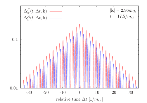
Figure 1: Statistical propagator $\Delta_{\varphi}^{F}=(\Delta_{\varphi}^{>}+\Delta_{\varphi}^{<})/2$ (red) and spectral function $\Delta_{\varphi}^{\cal A}=\frac{\rm i}{2}(\Delta_{\varphi}^{>}-\Delta_{\varphi}^{<})$ (blue) obtained from a numerical solution of the Kadanoff-Baym equations. Shown is the dependence on the relative time $\Delta t$ for fixed central time $t$.

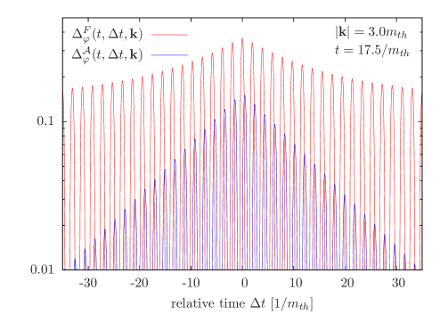
Figure 2: As figure 1, but for the excited momentum mode $|\mathbf{k}|=3.0m_{th}$. The statistical propagator $\Delta_{\varphi}^{F}=(\Delta_{\varphi}^{>}+\Delta_{\varphi}^{<})/2$ can be described by the sum of an exponentially damped equilibrium contribution and an undamped non-equilibrium contribution.

4 Out-of-Equilibrium Propagator from a Numerical Simulation

In this Section, we present a numerical check that indeed, when backreaction effects may be neglected, Eq. (50) is a correct solution to the Kadanoff-Baym equations, while the naïve finite-width ansatz (54) is not.

The assumption that is crucial for deriving the analytical solution (50,53) to the Kadanoff-Baym equations is the time-independence of the self-energy in Wigner space, $\Pi_{\varphi}(t,k_{\mu})=\Pi_{\varphi}(k_{\mu})$. This situation is realized for example when the non-equilibrium field $\varphi$ interacts with a thermal bath. In this case, a necessary condition for the time-independence of the self-energies is that the thermal bath can be considered as an infinitely large reservoir, that is not influenced itself by the interaction with the non-equilibrium field $\varphi$.

In this context the question arises how sensitive the analytical solution (50,53), and in particular the peculiar behaviour of the non-equilibrium contribution, is to the underlying thermal-bath assumption. In order to investigate this question, we compare the analytical expression with numerical solutions to the complete Kadanoff-Baym equations, for which the self-energies are computed self-consistently. This ensures that the full back-reaction is taken into account. Concretely, we consider a real scalar field with $\lambda\varphi^{4}$ interaction, and solve the Kadanoff-Baym equations in the two-time representation,

$$\left(\partial_{x}^{2}+m_{\varphi}^{2}+\frac{\lambda}{2}\Delta_{\varphi}^{<,>}(x,x)\right)\Delta_{\varphi}^{<,>}(x,y) = 2\int_{t_{0}}^{y^{0}}d^{4}z\,\Pi_{\varphi}^{<,>}(x,z)\Delta_{\varphi}^{\cal A}(z,y)$$

$${}-2\int_{t_{0}}^{x^{0}}d^{4}z\,\Pi_{\varphi}^{\cal A}(x,z)\Delta_{\varphi}^{<,>}(z,y)\;,$$

where $t_{0}$ is the initial time, $\Delta_{\varphi}^{\cal A}=\frac{\rm i}{2}(\Delta_{\varphi}^{>}-\Delta_{\varphi}^{<})$ is the spectral function, and

$$\int_{t_{0}}^{x^{0}}d^{4}z=\int_{t_{0}}^{x^{0}}dz^{0}\int d^{3}z\;.$$

For the self-energies, we use the so-called setting-sun approximation,

$$\Pi_{\varphi}^{<,>}(x,y)=-\frac{\lambda^{2}}{6}\Delta_{\varphi}^{<,>}(x,y)^{3}\;,$$ (56)

which describes scattering processes, and is accurate for small enough coupling and occupation numbers (see [42, 43] for details). We assume that the system is spatially homogeneous and isotropic. In this case it is convenient to transform to spatial momentum space,

$$\Delta_{\varphi}^{<,>}(t,\Delta t,|\mathbf{k}|)=\int d^{3}x\,e^{-{\rm i}\mathbf{k}\cdot(\mathbf{x}-\mathbf{y})}\,\Delta_{\varphi}^{<,>}(x,y)\;,$$ (57)

where, in addition, we have introduced the central time $t=(x^{0}+y^{0})/2$ and the relative time $\Delta t=x^{0}-y^{0}$ for convenience. The Wigner space functions would result by an additional Fourier transformation with respect to $\Delta t$.

Since we are interested in situations where a non-equilibrium degree of freedom interacts with many other degrees of freedom that are close to thermal equilibrium, we initialize the system at time $t=\Delta t=0$ with thermal correlators at temperature $T=1.5m_{th}$, where $m_{th}$ is the thermal mass. As described in [44], we also take the thermal non-Gaussian four-point correlation into account. In addition, one momentum mode, taken to be $|\mathbf{k}|=3.0m_{th}$, is excited above the thermal occupation with an effective particle number $\Delta n=7.5$ (see [42]). For the numerical solution we use a lattice of size $1400^{2}\times 32^{3}$ in $(x^{0},y^{0},\mathbf{k})$-space, a time-step $a_{t}=0.025/m_{th}$, and momentum cut-off $\Lambda=\pi/a_{x}$ with $a_{x}=0.5/m_{th}$. Furthermore, we choose $\lambda_{R}/4!=0.75$ for the renormalized coupling and determine the counterterms according to [45]. The numerical solutions conserve the total energy with an accuracy of better than $0.05\%$ (note that this property would be lost when neglecting the back-reaction).

The plots show the dependence of the two-point functions on the relative time $\Delta t$ for the excited momentum mode $|\mathbf{k}|=3.0m_{th}$, as well as a mode with slightly smaller momentum $|\mathbf{k}|=2.96m_{th}$. All correlators are evaluated at the fixed central time $t=17.5/m_{th}$. For the non-excited mode shown in Figure 1, we find that both the statistical propagator and the spectral function are damped exponentially with respect to the relative time, as expected. Furthermore, the damping rate is identical for both correlation functions. This property is expected from the fluctuation-dissipation relation which is valid in thermal equilibrium. In addition, the relative magnitude of the statistical propagator and the spectral function is close to the expected value $1+2f_{BE}(\sqrt{{\mathbf{k}}^{2}+m_{th}^{2}})\simeq 1.3$, where $f_{BE}$ is the Bose-Einstein distribution function.

In Figure 2, the corresponding propagators are shown for the excited momentum mode $|\mathbf{k}|=3.0m_{th}$. The spectral function is also damped exponentially, whereas the statistical propagator shows a different behaviour. However, the latter can be described to a good accuracy by the sum of the exponentially damped equilibrium contribution and an undamped non-equilibrium contribution. This is precisely the behaviour predicted by the analytical solution (50,53). In addition, we have checked that when varying the central time $t$, the non-equilibrium contribution to the statistical propagator decays exponentially, while the equilibrium contribution remains constant. In addition, the decay rate of the non-equilibrium contribution obtained in this way coincides with the damping rate of the equilibrium propagators. Again, this result is in accordance with the analytical solution (50,53). We conclude that the analytical solution obtained under the thermal bath assumption constitutes a reasonable approximation to the full numerical solutions, and is in particular consistent with a non-equilibrium correlator that is undamped with respect to the relative time.

5 Effectively Finite Width from the Gradient Expansion

We have now established analytically and numerically, that when backreaction may be neglected, the Wightman functions (50) that feature zero-width out-of-equilibrium contributions are indeed correct solutions to the Schwinger-Dyson equations on the CTP. In this Section, we investigate, whether the finite-width ansatz (54) for ${\rm i}\Delta_{\varphi}^{<,>}$, that we might intuitively expect and that it is often assumed in the literature, may yet be appropriate, and if yes, in what sense.

For this purpose, we substitute Eq. (50) into the right hand side of Eq. (44). The substitution results in

$$\sum\limits_{n=0}^{\infty}\frac{1}{n!}\left(-\frac{\rm i}{2}\Gamma_{\varphi}(\mathbf{k})\right)^{n}\left[(\partial_{k^{0}})^{n}\Pi_{\varphi}^{\cal A}\right]\delta f_{\varphi}(k^{0},\mathbf{k}){\rm sign}(k^{0})2\pi\delta(k^{2}-m_{\varphi}^{2}-\Pi_{\varphi}^{H}){\rm e}^{-\Gamma_{\varphi}(\mathbf{k})t}\,.$$ (58)

We now use the fact that we evaluate these terms in the distributional sense, after integration over $dk^{0}$, such that we can swap the $k^{0}$-derivatives through integration by parts. Therefore, within the $\delta$-functions, we replace $k^{0}\to k^{0}+\frac{\rm i}{2}\Gamma_{\varphi}$, because Eq. (58) corresponds to a Taylor series. One may worry about the fact that we have deliberately replaced expressions of $\Pi_{\varphi}^{\cal A}/k^{0}$ by $\Gamma_{\varphi}(\mathbf{k})$ and therefore truncated additional $k^{0}$ dependence. However, we may estimate derivatives with respect to $k^{0}$ acting on these factors as yielding factors of $T^{-1}$, such that the error incurred within each order $n$ of the gradient expansion can be estimated as $(\Gamma_{\varphi}(\mathbf{k})/T)^{n}$. The same argument applies to derivatives acting on $\delta f_{\varphi}(k^{0},k)$. Derivatives acting on ${\rm sign}(k^{0})$ are suppressed because $\delta(k^{2}-m_{\varphi}^{2}-\Pi_{\varphi}^{H})=0$ for $k^{0}=0$, at least provided $m_{\varphi}^{2}+\Pi_{\varphi}^{H}\not=0$. The suppression of gradients does obviously not apply to derivatives acting on the $\delta$-function. The consequences of this is what we explicitly calculate in the following.

From Eq. (53), we see that the $\delta$-function originates from the Fourier transform of $\cos(\omega_{\varphi}(\mathbf{k})\Delta t)$ with respect to $\Delta t$. The real part of Eq. (58) enters the kinetic equations (47b), while the imaginary part enters the constraint equations (47a). To this end, $k^{0}$ has been assumed to be real, while now, we aim to continue the expressions to complex $k^{0}$. This implies, that we need to identify the various occurrences with $k^{0}$ or ${k^{0}}^{*}$. The correct prescriptions are determined by the causal properties of the propagators, i.e. in two-time representation, whether the time argument is evaluated above or below the real axis, or in Wigner space, where the poles are located with respect to the real axis of the $k^{0}$-plane, cf. Appendix B for a quick reminder on this matter. In two-time representation, the correct prescription for the imaginary part of the time argument is given by

$$2\Delta^{\cal A}_{\rm eff}(k)= \frac{{\rm sign}(k^{0})}{\omega_{\varphi}(\mathbf{k})}\int\limits_{-\infty}^{\infty}d\,\Delta t\,{\rm e}^{({\rm i}k^{0}-\frac{1}{2}\Gamma_{\varphi}(\mathbf{k}){\rm sign}(\Delta t))\Delta t}\cos\left(\omega_{\varphi}\Delta t\right)$$ (59)

$$= \frac{{\rm sign}(k^{0})}{2\omega_{\varphi}(\mathbf{k})}\sum\limits_{\pm}\bigg{[}\frac{\rm i}{k^{0}\pm\omega_{\varphi}(\mathbf{k})+\frac{\rm i}{2}\Gamma_{\varphi}(\mathbf{k})}-\frac{\rm i}{k^{0}\pm\omega_{\varphi}(\mathbf{k})-\frac{\rm i}{2}\Gamma_{\varphi}(\mathbf{k})}\bigg{]}$$

$$= \frac{{\rm sign}(k^{0})}{\omega_{\varphi}(\mathbf{k})}\frac{\Gamma_{\varphi}(\mathbf{k})({k^{0}}^{2}+\omega_{\varphi}^{2}(\mathbf{k}))}{({k^{0}}^{2}-\omega_{\varphi}^{2}(\mathbf{k}))^{2}+[(k^{0}+\omega_{\varphi}(\mathbf{k}))^{2}+(k^{0}-\omega_{\varphi}^{2}(\mathbf{k}))^{2}]\frac{1}{4}\Gamma_{\varphi}^{2}(\mathbf{k})+\frac{1}{16}\Gamma_{\varphi}^{4}(\mathbf{k})}$$

$$\approx \frac{2\Gamma_{\varphi}(\mathbf{k})k^{0}}{({k^{0}}^{2}-\omega_{\varphi}^{2}(\mathbf{k}))^{2}+{k^{0}}^{2}\Gamma_{\varphi}^{2}(\mathbf{k})}\overset{\Gamma_{\varphi}\to 0}{=}{\rm sign}(k^{0})2\pi\delta({k^{0}}^{2}-\omega_{\varphi}^{2}(\mathbf{k}))\,.$$

This result is purely real, such that it enters into the kinetic equations, but not into the constraint equations. Note that for these equations to be valid the actual integration interval must be large compared to $\Gamma_{\varphi}^{-1}$. Regarding the replacement ${k^{0}}^{2}\to\omega^{2}_{\varphi}(\mathbf{k})$ in the numerator, one may worry that one drops a term that gives rise to relevant contributions to the integrations over $k^{0}$. Note however, that within the collision term, this finite width representation is always multiplied by distribution functions. We therefore assume, that all distribution functions decay exponentially for large values of $|k^{0}|$, as it is the case for e.g. the equilibrium distribution functions.

We also observe that

$$\Delta^{R}(k) =\frac{1}{k^{2}-m^{2}+{\rm i}\varepsilon k^{0}}\,,$$ (60a)

$$\Delta^{A}(k) =\left(\frac{1}{k^{2}-m^{2}+{\rm i}\varepsilon k^{0}}\right)^{*}\,,$$ (60b)

may be continued to complex $k^{0}$ with ${\rm Im}[k^{0}]>0$ while maintaining the causal properties, because these expressions are analytic in the upper complex half-plane. In terms of these propagators, we may express

$$2\Delta^{\cal A}=\frac{\rm i}{k^{2}-m_{\varphi}^{2}-\Pi_{\varphi}^{H}(k)+{\rm i}\varepsilon k^{0}}-\frac{\rm i}{(k^{2})^{*}-m_{\varphi}^{2}-\Pi_{\varphi}^{H}(k)-{\rm i}\varepsilon k^{0}}\,.$$ (61)

For real $k^{0}$ and infinitesimal $\varepsilon$, this corresponds to the representation of $2\pi\delta(k^{2}-m_{\varphi}^{2}-\Pi^{H}_{\varphi}(k))=2\Delta^{(0){\cal A}}$ as in Eq. (58). Through the Taylor expansion, this expression can be directly continued to complex arguments as $k^{0}\to k^{0}+\frac{\rm i}{2}\Gamma_{\varphi}(\mathbf{k})$

$$\Delta^{\cal A}_{\rm eff}(k^{0},\mathbf{k})=\Delta^{(0){\cal A}}\left(k^{0}+\frac{\rm i}{2}\Gamma_{\varphi}(\mathbf{k}),\mathbf{k}\right)\,,$$ (62)

in agreement with Eq. (59).

It should be noted that due to the singular behaviour of the on-shell $\delta$-functions, it is not consistent to truncate the gradient expansion of the collision term at any finite order in the diamond operator. Here, we have shown that the gradients can easily be resummed to yield a benign contribution with an intuitively clear meaning: an effective finite-width distribution function. We therefore expect that the systematics of the gradient expansion still applies to kinetic theory, once singular terms arising from on-shell $\delta$-functions are summed, following the methods introduced in the present Section.

In conclusion, the higher order contributions from the gradient expansion that arise within the collision term precisely recover the naïve finite-width ansatz (54)! In this sense, the fluctuation-dissipation relation generalises to an out-of-equilibrium system of the scalar field $\varphi$, for which backreaction can be neglected. In turn, when we substitute the finite width ansatz (54) into the collision term, we must not expand to higher orders in gradients, as this is already accounted for by the ansatz itself.

6 Application to Processes with Kinematic Thresholds

Provided the self-energy $\Pi_{\varphi}(k)$ is not changing rapidly in $k^{0}$ close to the pole, there is no leading order difference in whether we integrate over the $\delta$-function or the finite width representation of the propagator. This behaviour is however precisely what we assume within the Breit-Wigner approximation (51). Moreover, when we integrate the kinetic equation (47b) for $k^{0}$ from $-\infty$ to $\infty$, both sides are trivially zero, because of the symmetry properties of the real field. Hence, in order to “measure” the effectively finite width behaviour found in the previous Section, we yet need to specify an interaction that can probe the off-shell contributions of ${\rm i}\Delta^{<,>}_{\varphi}(k)$ for $k^{0}\not=\omega_{\varphi}(\mathbf{k})$.

We therefore consider a reaction that is mediated by a coupling $h$ and that is kinematically forbidden at tree-level. For such a process, accounting for the effective finite width of the propagators is indeed of leading order importance. Second, in order to extract non-trivial information about the kinetic evolution, instead of plainly integrating over $k^{0}$, one needs to include integrals over higher moments (additional powers of $k^{0}$ within the integrand). For example, the distribution function can be obtained from the integral

$$f_{\varphi}(\mathbf{k})=\int\frac{dk^{0}}{2\pi}|k^{0}|{\rm i}\Delta_{\varphi}^{<}(k)-\frac{1}{2}\,.$$ (63)

For different observables, analogous prefactors for ${\rm i}\Delta_{\varphi}^{<}$ can be found that are typically smooth functions of $k^{0}$ in the vicinity of the quasi-particle pole, such that derivatives may be consistently neglected at leading order in the gradient expansion.

For the purpose of probing the width of the field $\varphi$, we introduce two additional scalar fields $\chi_{1,2}$. The equation that determines the evolution of $f_{\chi_{1}}$ follows from the kinetic equation (47b) (with the obvious replacement $\varphi\to\chi_{1}$) as

$$\partial_{t}f_{\chi_{1}}(\mathbf{k})= \int\frac{dk^{0}}{2\pi}|k^{0}|\partial_{t}{\rm i}\Delta^{<,>}_{\chi_{1}}$$ (64)

$$= -\int\frac{dk^{0}}{2\pi}{\rm sign}(k^{0})\frac{1}{2}\cos(\diamond)\left(\{{\rm i}\Pi_{\chi_{1}}^{>}\}\{{\rm i}\Delta_{\chi_{1}}^{<}\}-\{{\rm i}\Pi_{\chi_{1}}^{<}\}\{{\rm i}\Delta_{\chi_{1}}^{>}\}\right)\,.$$

Here, we have truncated terms that are of higher order in gradients on the left-hand side.

In the presence of kinematic thresholds, including the gradient terms that lead to the effective finite width can be of leading importance. In order to illustrate this, we consider an interaction described by the Lagrangian term $h\varphi\chi_{1}\chi_{2}$, where $h$ is a real dimensionful coupling constant. For the field $\chi_{1}$, this induces the Wightman-type self-energies

$${\rm i}\Pi_{\chi_{1}}^{<,>}(k)=h^{2}\int\frac{d^{4}p}{(2\pi)^{4}}{\rm i}\Delta_{\varphi}^{<,>}(k-p){\rm i}\Delta_{\chi_{2}}^{<,>}(p)\,.$$ (65)

Suppose now, that the field $\varphi$ deviates from equilibrium, as described by the distribution function $\delta f_{\varphi}(\mathbf{p})$, while the fields $\chi_{1,2}$ are in equilibrium at the temperature $T$. The fields have the masses $m_{\varphi}$ and $m_{\chi_{1,2}}$. Moreover, assume that the production or decay rates of $\chi_{1,2}$ due to the interaction with $\varphi$ are much smaller than the decay rate $\Gamma_{\varphi}$. Then, we can use for ${\rm i}\Delta_{\chi_{1,2}}$ the on-shell propagators. Moreover, the leading time dependence is in $\delta f_{\varphi}(\mathbf{p})$, and we may evaluate the action of the diamond operators as

$$\partial_{t}f_{\chi_{1}}(\mathbf{k})= -\frac{1}{2}h^{2}{\rm Re}\bigg{[}\sum\limits_{n=0}^{\infty}\int\frac{d^{3}p}{(2\pi)^{3}}\int\frac{dk^{0}}{2\pi}\int\frac{dp^{0}}{2\pi}$$ (66)

$${\rm i}\Delta_{\chi_{2}}^{>}(p)\frac{1}{n!}\left(\left[\frac{\rm i}{2}\partial_{t}\right]^{n}{\rm i}\Delta^{>}_{\varphi}(k-p)\right)\partial_{k^{0}}^{n}{\rm i}\Delta_{\chi_{1}}^{<}(k){\rm sign}(k^{0})\bigg{]}-(<,>\leftrightarrow>,<)\,.$$

We could now directly apply the Taylor expansion to the propagator $\Delta_{\chi_{1}}$. However, since it is the field $\varphi$ which is the origin of the effective finite width behaviour, we rather perform an integration by parts, in order to attach the derivatives $\partial_{k^{0}}$ to ${\rm i}\Delta_{\varphi}$. We again ignore derivatives acting on $\Gamma_{\varphi}$, since these would lead to terms that are suppressed by higher orders in the gradient expansion. Note also that we can ignore the derivatives acting on the sign function, since the on-shell propagator ${\rm i}\Delta_{\chi_{1}}(k)$ vanishes for $k^{0}=0$.

Substituting the explicit forms of the propagator and performing the Taylor expansion of ${\rm i}\Delta_{\varphi}(k-p)$ toward complex $k^{0}$, as it is explained in the previous Section, we obtain

$$\partial_{t}f_{\chi_{1}}(\mathbf{k})= \frac{1}{2}h^{2}\int\frac{d^{3}p}{(2\pi)^{3}}\int\frac{dk^{0}}{2\pi}\int\frac{dp^{0}}{2\pi}{\rm sign}(p^{0})2\pi\delta(p^{2}-m_{\chi_{2}}^{2})2\pi\delta(k^{2}-m_{\chi_{1}}^{2})$$ (67)

$$\times \frac{2\Gamma_{\varphi}(\mathbf{k}-\mathbf{p})\omega_{\varphi}(\mathbf{k}-\mathbf{p})}{[(k-p)^{2}-m_{\varphi}^{2}]^{2}+(k^{0}-p^{0})^{2}\Gamma_{\varphi}^{2}}\delta f_{\varphi}(\mathbf{k}-\mathbf{p}){\rm e}^{-\Gamma_{\varphi}(\mathbf{k}-\mathbf{p})t}\left[\frac{1}{{\rm e}^{p^{0}/T}-1}-\frac{1}{{\rm e}^{k^{0}/T}-1}\right].$$

Now assume for definiteness, that $m_{\chi_{1}}+m_{\chi_{2}}>m_{\varphi}$ but $m_{\chi_{1,2}}+m_{\varphi}>m_{\chi_{2,1}}$. This is for example the case when all masses are of equal or similar size. A $1\leftrightarrow 2$ process between $\varphi$ and $\chi_{1,2}$ then is not possible provided all particles are on-shell. In the present case, the field $\varphi$ obtains an effective finite width, and $\partial_{t}f_{\chi_{1}}(\mathbf{k})$ is non-zero, even for the given mass relations. The above integral can in general be evaluated numerically in a straightforward way. Let us however additionally assume that $m_{\chi_{1,2}},m_{\varphi}\gg T$ and $m_{\chi_{1}}+m_{\chi_{2}}-m_{\varphi}\ll m_{\chi_{1,2}},m_{\varphi}$. In that situation, all particles are non-relativistic such that $\omega_{\chi_{1,2},\varphi}(\mathbf{k})\approx m_{\chi_{1,2},\varphi}$ and $\Gamma_{\varphi}(\mathbf{k})\approx\Gamma_{\varphi}(\mathbf{0})$. Moreover, the dominant reaction channel is $\chi_{1}+\chi_{2}\leftrightarrow\varphi$, where $\varphi$ is off-shell. The meaning of $\varphi$ being off shell is that it corresponds to a virtual state, that eventually rescatters with addtional particles, which is encompassed within the self-energy $\Pi^{\cal A}_{\varphi}$. In this situation, the angular integration can be performed easily. Moreover, we note that in the integrand ${\rm sign}(p^{0})\not={\rm sign}(k^{0})$. With the above approximations, we therefore obtain

$$\partial_{t}f_{\chi_{1}}(\mathbf{k})\!\approx \frac{1}{2}h^{2}\!\frac{1}{2\omega_{\chi_{1}}(\mathbf{k})}\!\!\int\limits_{0}^{\infty}\!\frac{p^{2}dp}{(2\pi)^{2}}\frac{1}{2\omega_{\chi_{2}}(\mathbf{p})}\frac{4\Gamma_{\varphi}(\mathbf{0})m_{\varphi}}{\left[m_{\chi_{1}}^{2}\!+m_{\chi_{2}}^{2}\!-m_{\varphi}^{2}+2m_{\chi_{1}}m_{\chi_{2}}\right]^{2}\!+(m_{\chi_{1}}\!+m_{\chi_{2}})^{2}\Gamma_{\varphi}^{2}}$$

$$\times \int\limits_{-1}^{1}d\cos{\vartheta}\,\delta f_{\varphi}(\mathbf{k}-\mathbf{p}){\rm e}^{-\Gamma_{\varphi}(\mathbf{0})t}\,,$$ (68)

where $\vartheta$ is the angle between $\mathbf{k}$ and $\mathbf{p}$ and where we have assumed that $\delta f_{\varphi}(\mathbf{k})$ is isotropic. Clearly, this can be interpreted as a scattering process, between $\varphi$ and additional particles, that are described by $\Gamma_{\varphi}$, via a virtual off-shell $\varphi$ into $\chi_{1}$ and $\chi_{2}$. In contrast, the result would be strictly zero if we would not have taken account of the resummation leading to the effective finite width propagator as discussed in the previous Section. We emphasise that for the present calculation, it is sufficient to take the Breit-Wigner approximation for $\Pi^{\cal A}_{\varphi}(k)$, while the dependence of $\Pi^{<,>}_{\chi_{1}}(k)$ on $k^{0}$ is of leading importance. For related discussions of off-shell effects, cf. Refs. [37, 13].

7 Conclusions

For an out-of equilibrium scalar field, that interacts with a time-independent, spatially homogeneous bath and that only experiences negligible backreaction, we have reviewed and derived various aspects of the solutions to the Schwinger-Dyson equations on the CTP. Our main focus is the solution for the Wightman function (50) and its curious feature, that it decomposes into a finite-width equilibrium and a zero-width out-of-equilibrium contribution. The corresponding Wightman function has been derived before in position space in Ref. [11], but no direct interpretation of the different width of the two components is provided there. The fact that the equilibrium component exhibits a finite width is confirmed by a direct summation of the geometric series of insertions of the self-energies into the propagators. This calculation has first been performed in Ref [33], and in Section 2 we have reviewed it in order to put it within the present context. The desirable cancellation of pinch singularities is accompanied by a spectacular cancellation of the out-of-equilibrium contributions. In order to verify that the vanishing width of the out-of equilibrium component is not an artefact of the analytical approximations, in Section 4, we have presented a numerical study that clearly confirms this feature. We emphasise that when using the Schwinger-Dyson approach, we do not encounter a problem with pinch singularities. Besides, we do not find a breakdown of perturbation theory applied to out-of-equilibrium systems, that is sometimes associated with pinch singularities [34, 35].

The zero width behaviour of the out-of-equilibrium Wightman function, that we have carefully confirmed calls for interpretation. Intuitively, we expect that it should not be distinguishable, whether a quasi-particle is part of the equilibrium or out-of-equilibrium distribution. In Section 5, we present the observation, that an effective finite width for the out-of-equilibrium contribution results from a summation of all gradients within the collision term. Such a summation to all orders in gradients becomes necessary, because derivatives acting on the on-shell $\delta$-function are not suppressed and therefore do not comply with the usual suppression of higher orders derivatives in the gradient expansion. Section 6 provides an example, how the effective finite width is observable through interactions, that are kinematically forbidden for zero-width particles. Since the effective finite width takes the same form as the width of the equilibrium propagator, our findings may be interpreted as a generalisation of the fluctuation-dissipation relation to out-of-equilibrium systems with negligible backreaction.

The results of the present work provide a justification for the use of a heuristic finite-width ansatz, that is often intuitively applied within kinetic theory, e.g. in Refs. [16, 17, 18, 19, 20, 21, 36, 37]. If one aims to derive kinetic theory from first principles of Quantum Field Theory, using the CTP formalism, the present work fills in a missing step in order to describe the finite width of out-of-equilibrium particles. Note that the propagators for fermions reported in Refs. [12, 14] also feature a zero-width non-equilibrium contribution. The resummation technique leading to an effective finite width can in principle be generalised to fermionic systems.

In the field of leptogenesis, we see future applications in studying the role of the finite width of the singlet neutrino, a discussion which has been initiated in Refs. [12, 14]. Moreover, the correct description of the finite width of out-of-equilibrium neutrinos is potentially crucial for resonant leptogenesis [46, 47, 48, 49, 50] in a regime, where the poles of the nearly mass-degenerate neutrinos overlap within their width.

In conclusion, we have shown that the Schwinger-Dyson equations on the CTP in the linear approximation, that allows for analytical solutions, are well suited to describe finite-width effects for out-of-equilibrium systems. Due to the zero-width behaviour of the Wightman functions, this is not directly obvious, and to arrive at this result, a non-trivial summation of gradients of all orders acting on on-shell $\delta$-functions is necessary. Once this summation is performed, it appears that the usual gradient expansion can be systematically extended order by order. In the future, we may therefore expect further progress in the application of the CTP formalism to the analytical description of out-of-equilibrium systems.

Appendix A Two Point Functions on the CTP and Wigner Space

Within the present work, we follow the notations and conventions as given in Ref. [9]. For a quick reference, we quote here the relations between the two-point functions, that are used within the present work, where $G$ may either stand for a CTP Green function $\Delta$ or a self-energy $\Pi$:

$$G^{A}=G^{T}-G^{>}=G^{<}-G^{\bar{T}}\quad \textnormal{(advanced)}\,,$$ (69a)

$$G^{R}=G^{T}-G^{<}=G^{>}-G^{\bar{T}}\quad \textnormal{(retarded)}\,,$$ (69b)

$$G^{H}=\frac{1}{2}(G^{R}+G^{A})\quad \textnormal{(Hermitian)}\,,$$ (69c)

$$G^{\cal A}=\frac{1}{2\rm i}(G^{A}-G^{R})=\frac{\rm i}{2}(G^{>}-G^{<})\quad \textnormal{(anti-Hermitian, spectral)}\,.$$ (69d)

The identification of these two-point functions with those bearing CTP indices is

$$G^{T}=G^{++}\,,\quad G^{<}=G^{+-}\,,\quad G^{>}=G^{-+}\,,\quad G^{\bar{T}}=G^{--}\,.$$ (70)

The functions $G^{<,>}$ are known as the Wightman functions, $G^{T}$ is time ordered, $G^{\bar{T}}$ anti-time ordered.

The Wigner transform of a two-point function is defined as

$$G(k,x)=\int d^{4}r{\rm e}^{{\rm i}kr}G(x+r/2,x-r/2)\,,$$ (71)

where we refer to $r$ as the relative and to $x$ as the average coordinate. In the situation of spatial homogeneity, there is no dependence on $\mathbf{x}$ (spatial translation invariance), such that $G(k,x)\equiv G(k,t)$.

Appendix B Prescription for the Imaginary Part of the Time Argument

The time-ordered and anti-time ordered Green functions of a scalar field $\varphi$ are

$${\rm i}\Delta^{T,\bar{T}}(\Delta x)= \int\frac{d^{4}p}{(2\pi)^{4}}{\rm e}^{-{\rm i}p\cdot\Delta x}\frac{\rm i}{{p^{0}}^{2}-\omega^{2}_{\varphi}(\mathbf{p})\pm{\rm i}\varepsilon}$$ (72)

$$= \int\frac{d^{3}p}{(2\pi)^{3}2\omega_{\varphi}(\mathbf{p})}\bigg{\{}\pm{\rm e}^{{\rm i}(\omega_{\varphi}(\mathbf{k})\mp{\rm i}\varepsilon)\Delta x^{0}}\vartheta(\mp\Delta x^{0})\pm{\rm e}^{-{\rm i}(\omega_{\varphi}(\mathbf{k})\mp{\rm i}\varepsilon)\Delta x^{0}}\vartheta(\pm\Delta x^{0})\bigg{\}}{\rm e}^{{\rm i}\mathbf{p}\cdot\Delta\mathbf{x}}\,.$$

Thus, the prescription for the imaginary part always appears in such a way that the integrand decays exponentially for large $|\Delta x^{0}|$. Also recall that we may write ${\rm i}\Delta^{<,>}(\Delta x)=\vartheta(\Delta x){\rm i}\Delta^{\bar{T},T}(\Delta x)+\vartheta(-\Delta x){\rm i}\Delta^{T,\bar{T}}(\Delta x)$. This explains the explicit appearance of ${\rm sign}(\Delta t)$ within Eq. (59).

References

- [1] J. S. Schwinger, “Brownian motion of a quantum oscillator,” J. Math. Phys. 2 (1961) 407.
- [2] L. V. Keldysh, “Diagram technique for nonequilibrium processes,” Zh. Eksp. Teor. Fiz. 47 (1964) 1515 [Sov. Phys. JETP 20 (1965) 1018].
- [3] E. Calzetta and B. L. Hu, “Nonequilibrium Quantum Fields: Closed Time Path Effective Action, Wigner Function and Boltzmann Equation,” Phys. Rev. D 37 (1988) 2878.
- [4] K. -C. Chou, Z. -B. Su, B. -L. Hao, L. Yu, “Equilibrium and Nonequilibrium Formalisms Made Unified,” Phys. Rept. 118 (1985) 1.
- [5] J. Berges, “Introduction to nonequilibrium quantum field theory,” AIP Conf. Proc. 739 (2005) 3-62. [hep-ph/0409233].
- [6] J. M. Maldacena, “Non-Gaussian features of primordial fluctuations in single field inflationary models,” JHEP 0305 (2003) 013. [astro-ph/0210603].
- [7] E. Calzetta, B. L. Hu, “Stochastic dynamics of correlations in quantum field theory: From Schwinger-Dyson to Boltzmann-Langevin equation,” Phys. Rev. D61 (2000) 025012. [hep-ph/9903291].
- [8] J. Berges, “N-particle irreducible effective action techniques for gauge theories,” Phys. Rev. D70 (2004) 105010. [hep-ph/0401172].
- [9] T. Prokopec, M. G. Schmidt and S. Weinstock, “Transport equations for chiral fermions to order h-bar and electroweak baryogenesis,” Annals Phys. 314 (2004) 208 [arXiv:hep-ph/0312110].
- [10] T. Prokopec, M. G. Schmidt and S. Weinstock, “Transport equations for chiral fermions to order h-bar and electroweak baryogenesis. II,” Annals Phys. 314 (2004) 267 [arXiv:hep-ph/0406140].
- [11] A. Anisimov, W. Buchmüller, M. Drewes and S. Mendizabal, “Nonequilibrium Dynamics of Scalar Fields in a Thermal Bath,” Annals Phys. 324 (2009) 1234 [arXiv:0812.1934 [hep-th]].
- [12] A. Anisimov, W. Buchmüller, M. Drewes and S. Mendizabal, “Leptogenesis from Quantum Interference in a Thermal Bath,” Phys. Rev. Lett. 104 (2010) 121102 [arXiv:1001.3856 [hep-ph]].
- [13] M. Drewes, “On the Role of Quasiparticles and thermal Masses in Nonequilibrium Processes in a Plasma,” arXiv:1012.5380 [hep-th].
- [14] A. Anisimov, W. Buchmüller, M. Drewes and S. Mendizabal, “Quantum Leptogenesis I,” arXiv:1012.5821 [hep-ph].
- [15] E. Calzetta and B. L. Hu, “Nonequilibrium Quantum Field Theory”, Cambridge University Press, Cambridge, UK (2008).
- [16] P. B. Arnold, G. D. Moore, L. G. Yaffe, “Transport coefficients in high temperature gauge theories. 1. Leading log results,” JHEP 0011 (2000) 001. [hep-ph/0010177].
- [17] P. B. Arnold, G. D. Moore, L. G. Yaffe, “Photon emission from ultrarelativistic plasmas,” JHEP 0111 (2001) 057. [hep-ph/0109064].
- [18] P. B. Arnold, G. D. Moore, L. G. Yaffe, “Photon emission from quark gluon plasma: Complete leading order results,” JHEP 0112 (2001) 009. [hep-ph/0111107].
- [19] P. B. Arnold, G. D. Moore, L. G. Yaffe, “Photon and gluon emission in relativistic plasmas,” JHEP 0206 (2002) 030. [hep-ph/0204343].
- [20] P. B. Arnold, G. D. Moore, L. G. Yaffe, “Effective kinetic theory for high temperature gauge theories,” JHEP 0301 (2003) 030. [hep-ph/0209353].
- [21] P. B. Arnold, G. DMoore, L. G. Yaffe, “Transport coefficients in high temperature gauge theories. 2. Beyond leading log,” JHEP 0305 (2003) 051. [hep-ph/0302165].
- [22] T. Konstandin, T. Prokopec, M. G. Schmidt and M. Seco, “MSSM electroweak baryogenesis and flavour mixing in transport equations,” Nucl. Phys. B 738 (2006) 1 [arXiv:hep-ph/0505103].
- [23] V. Cirigliano, C. Lee, M. J. Ramsey-Musolf, S. Tulin, “Flavored Quantum Boltzmann Equations,” Phys. Rev. D81 (2010) 103503. [arXiv:0912.3523 [hep-ph]].
- [24] M. Garny, A. Hohenegger, A. Kartavtsev and M. Lindner, “Systematic approach to leptogenesis in nonequilibrium QFT: vertex contribution to the CP-violating parameter,” Phys. Rev. D 80 (2009) 125027 [arXiv:0909.1559 [hep-ph]].
- [25] M. Garny, A. Hohenegger, A. Kartavtsev and M. Lindner, “Systematic approach to leptogenesis in nonequilibrium QFT: self-energy contribution to the CP-violating parameter,” Phys. Rev. D 81 (2010) 085027 [arXiv:0911.4122 [hep-ph]].
- [26] M. Garny, A. Hohenegger, A. Kartavtsev, “Medium corrections to the CP-violating parameter in leptogenesis,” Phys. Rev. D81 (2010) 085028. [arXiv:1002.0331 [hep-ph]].
- [27] M. Beneke, B. Garbrecht, M. Herranen and P. Schwaller, “Finite Number Density Corrections to Leptogenesis,” Nucl. Phys. B 838 (2010) 1 [arXiv:1002.1326 [hep-ph]].
- [28] M. Beneke, B. Garbrecht, C. Fidler, M. Herranen and P. Schwaller, “Flavoured Leptogenesis in the CTP Formalism,” Nucl. Phys. B 843 (2011) 177 [arXiv:1007.4783 [hep-ph]].
- [29] M. Garny, A. Hohenegger and A. Kartavtsev, “Quantum corrections to leptogenesis from the gradient expansion,” arXiv:1005.5385 [hep-ph].
- [30] B. Garbrecht, “Leptogenesis: The Other Cuts,” Nucl. Phys. B847 (2011) 350-366. [arXiv:1011.3122 [hep-ph]].
- [31] V. Cirigliano, C. Lee, S. Tulin, “Resonant Flavor Oscillations in Electroweak Baryogenesis,” [arXiv:1106.0747 [hep-ph]].
- [32] C. Greiner and S. Leupold, “Stochastic interpretation of Kadanoff-Baym equations and their relation to Langevin processes,” Annals Phys. 270 (1998) 328 [arXiv:hep-ph/9802312].
- [33] T. Altherr, “Resummation of perturbation series in nonequilibrium scalar field theory,” Phys. Lett. B 341 (1995) 325 [arXiv:hep-ph/9407249].
- [34] C. Greiner, S. Leupold, “Interpretation and resolution of pinch singularities in nonequilibrium quantum field theory,” Eur. Phys. J. C8 (1999) 517-522. [hep-ph/9804239].
- [35] D. Boyanovsky, H. J. de Vega, S. -Y. Wang, “Dynamical renormalization group approach to quantum kinetics in scalar and gauge theories,” Phys. Rev. D61 (2000) 065006. [hep-ph/9909369].
- [36] S. Mrowczynski, “Transport theory of massless fields,” Phys. Rev. D56 (1997) 2265-2280. [hep-th/9702022].
- [37] B. Garbrecht and T. Konstandin, “Separation of Equilibration Time-Scales in the Gradient Expansion,” Phys. Rev. D 79 (2009) 085003 [arXiv:0810.4016 [hep-ph]].
- [38] A. Anisimov, D. Besak and D. Bödeker, “Thermal production of relativistic Majorana neutrinos: Strong enhancement by multiple soft scattering,” arXiv:1012.3784 [hep-ph].
- [39] M. Herranen, K. Kainulainen and P. M. Rahkila, “Kinetic theory for scalar fields with nonlocal quantum coherence,” JHEP 0905 (2009) 119 [arXiv:0812.4029 [hep-ph]].
- [40] M. Herranen, K. Kainulainen and P. M. Rahkila, “Quantum kinetic theory for fermions in temporally varying backrounds,” JHEP 0809 (2008) 032 [arXiv:0807.1435 [hep-ph]].
- [41] M. Herranen, K. Kainulainen and P. M. Rahkila, “Towards a kinetic theory for fermions with quantum coherence,” Nucl. Phys. B 810 (2009) 389 [arXiv:0807.1415 [hep-ph]].
- [42] M. Lindner, M. M. Müller, “Comparison of Boltzmann equations with quantum dynamics for scalar fields,” Phys. Rev. D73 (2006) 125002. [hep-ph/0512147].
- [43] J. Berges, J. Cox, “Thermalization of quantum fields from time reversal invariant evolution equations,” Phys. Lett. B517 (2001) 369-374. [hep-ph/0006160]; G. Aarts, J. Berges, “Classical aspects of quantum fields far from equilibrium,” Phys. Rev. Lett. 88 (2002) 041603. [hep-ph/0107129]; S. Juchem, W. Cassing, C. Greiner, “Quantum dynamics and thermalization for out-of-equilibrium theory,” Phys. Rev. D69 (2004) 025006. [hep-ph/0307353]; A. Arrizabalaga, J. Smit, A. Tranberg, “Equilibration in theory in 3+1 dimensions,” Phys. Rev. D72 (2005) 025014. [hep-ph/0503287].
- [44] M. Garny, M. M. Müller, “Kadanoff-Baym Equations with Non-Gaussian Initial Conditions: The Equilibrium Limit,” Phys. Rev. D80 (2009) 085011. [arXiv:0904.3600 [hep-ph]].
- [45] J. Berges, S. .Borsanyi, U. Reinosa, J. Serreau, “Renormalized thermodynamics from the 2PI effective action,” Phys. Rev. D71 (2005) 105004. [hep-ph/0409123]; J. Berges, S. Borsanyi, U. Reinosa, J. Serreau, “Nonperturbative renormalization for 2PI effective action techniques,” Annals Phys. 320 (2005) 344-398. [hep-ph/0503240].
- [46] M. Flanz, E. A. Paschos and U. Sarkar, “Baryogenesis from a lepton asymmetric universe,” Phys. Lett. B 345 (1995) 248 [Erratum-ibid. B 382 (1996) 447] [arXiv:hep-ph/9411366].
- [47] M. Flanz, E. A. Paschos, U. Sarkar and J. Weiss, “Baryogenesis through mixing of heavy Majorana neutrinos,” Phys. Lett. B 389 (1996) 693 [arXiv:hep-ph/9607310].
- [48] A. Pilaftsis, “CP violation and baryogenesis due to heavy Majorana neutrinos,” Phys. Rev. D 56 (1997) 5431 [arXiv:hep-ph/9707235].
- [49] L. Covi, E. Roulet and F. Vissani, “CP violating decays in leptogenesis scenarios,” Phys. Lett. B 384 (1996) 169 [arXiv:hep-ph/9605319].
- [50] A. Pilaftsis and T. E. J. Underwood, “Resonant Leptogenesis,” Nucl. Phys. B 692 (2004) 303 [arXiv:hep-ph/0309342].
- [51] C. Fidler, M. Herranen, K. Kainulainen, P. M. Rahkila, “Flavoured quantum Boltzmann equations from cQPA,” [arXiv:1108.2309 [hep-ph]].