Finite Element Error Estimates for Critical Growth Semilinear Problems without Angle Conditions

Abstract.

In this article we consider a priori error and pointwise estimates for finite element approximations of solutions to semilinear elliptic boundary value problems in $d\geqslant 2$ space dimensions, with nonlinearities satisfying critical growth conditions. It is well-understood how mesh geometry impacts finite element interpolant quality, and leads to the reasonable notion of shape regular simplex meshes. It is also well-known how to perform both mesh generation and simplex subdivision, in arbitrary space dimension, so as to guarantee the entire hierarchy of nested simplex meshes produced through subdivision continue to satisfy shape regularity. However, much more restrictive angle conditions are needed for basic a priori quasi-optimal error estimates, as well as for a priori pointwise estimates. These angle conditions, which are particularly difficult to satisfy in three dimensions in any type of unstructured or adaptive setting, are needed to gain pointwise control of the nonlinearity through discrete maximum principles. This represents a major gap in finite element approximation theory for nonlinear problems on unstructured meshes, and in particular for adaptive methods. In this article, we close this gap in the case of semilinear problems with critical or sub-critical nonlinear growth, by deriving a priori estimates directly, without requiring the discrete maximum principle, and hence eliminating the need for restrictive angle conditions. Our main result is a type of local Lipschitz property that relies only on the continuous maximum principle, together with the growth condition. We also show that under some additional smoothness assumptions, the a priori error estimate itself is enough to give $L^{\infty}$ control the discrete solution, without the need for restrictive angle conditions. Numerical experiments confirm our theoretical conclusions.

1. Introduction

In this article we consider a priori error estimates and discrete pointwise estimates for Galerkin finite element approximation of solutions to a general class of semilinear problems satisfying certain growth conditions in $d$ space dimensions, which includes problems with critical and subcritical polynomial nonlinearity. When $d=2$ and $d=3$, it is well-understood how mesh geometry impacts finite element interpolant quality (cf. [3]). Such considerations lead to the requirement that simplex meshes used for finite element approximation satisfy a reasonable mesh condition known as shape regularity. It is well-known how to perform both mesh generation and simplex subdivision, in arbitrary space dimension, so as to guarantee that the entire hierarchy of nested simplex meshes produced through subdivision satisfy shape regularity, and continue to do so asymptotically (cf. [1, 4, 5, 29]). However, much more restrictive angle conditions are needed for basic a priori quasi-optimal error estimates, as well as for a priori pointwise estimates for Galerkin finite element approximations. These angle conditions, which are particularly difficult to satisfy in three dimensions in any type of unstructured or adaptive setting, are needed to gain pointwise control of the nonlinearity through discrete maximum principles. This represents a major gap in finite element approximation theory for nonlinear problems on unstructured meshes, and in particular for adaptive methods. In this article, we close this gap in the case of semilinear problems with critical or sub-critical nonlinear growth, by deriving a priori estimates directly (both error estimates and discrete pointwise estimates), without requiring the discrete maximum principle, and hence eliminating the need for restrictive angle conditions.

Critical exponent problems arise in a fundamental way throughout geometric analysis and general relativity. One of the seminal critical exponent problems in nonlinear PDE is the Yamabe Problem [2]: Find $u\in X$ (for some appropriate space $X$) such that

$$-8\Delta_{g}u+Ru =R_{u}u^{5}\quad\mbox{ in }\Omega,$$ (1.1)

$$u >0,$$ (1.2)

where $\Omega$ is a Riemannian $3$-manifold, $g$ is the positive definite metric on $\Omega$, $\Delta_{g}$ is the Laplace-Beltrami operator generated by $g$, $R$ is the scalar curvature of $g$, and $R_{u}$ is the scalar curvature corresponding to the conformally transformed metric: $\overline{g}=\phi^{4}g.$ The coefficients $R$ and $R_{u}$ can take any sign. The Banach space $X$ containing the solution is an appropriate Sobolev class $W^{s,p}(\Omega)$ for suitably chosen exponents $s$ and $p$. If the manifold $\Omega$ has a boundary, then boundary conditions are also prescribed, such as $u=1$ on an exterior boundary to $\Omega$. In the case that ${\Omega\subset\mathbb{R}^{3}}$, and ${g_{ij}=\delta_{ij}}$, then $\Delta_{g}$ reduces to just the Laplace operator on $\Omega$. This problem is full of features that are challenging both mathematically and numerically, including: critical exponent nonlinearity, potentially non-monotone nonlinearity, spatial dimension $d\geqslant 3$, and spatial domains that are typically non-flat Riemannian manifolds rather than simply open sets in $\mathbb{R}^{d}$. A related critical exponent problem, containing all of the difficulties of (1.1)–(1.2), plus the addition of low-order non-polynomial rational nonlinearities, arises in mathematical general relativity in the form of the Hamiltonian constraint equation; cf. [21].

The presence of the term $u^{5}$ term in (1.1), and in the related Hamiltonian constraint in general relativity, is an example of a critical exponent problem in space dimension three; such problems are known to be difficult to analyze due to the loss of compactness of the embedding ${H^{1}\subset L^{p+1}}$, where the dimension-dependent critical exponent ${p=(d+2)/(d-2)}$ takes value $p=5$ when $d=3$. Loss of compactness of the embedding creates obstacles that prevent the use of compactness arguments in standard variational, Galerkin, and fixed-point techniques. As a result, these techniques are generally restricted to subcritical nonlinearities, unless additional techniques give control of the nonlinearity, such as a priori $L^{\infty}$, or pointwise, control of solutions. The inequality constraint (1.2) creates additional complexities in both theory and numerical treatment of such problems, with only positive solutions having physical meaning. Prior work on numerical methods for critical exponent semilinear problems has focused primarily on the development of adaptive methods for recovering solution blowup; cf. [8, 7].

The standard approach to obtaining a priori $L^{\infty}$ bounds on Galerkin approximations is to enforce approximation space properties to guarantee discrete maximum principles, leading to geometrical conditions on the underlying simplex mesh. In the case of the $d=2$ Poisson problem, discrete maximum principles can be established if all angles in the triangulation are non-obtuse (cf. [12]). This was relaxed to “summation of two opposite angles less or equal to $\pi$” in [42, Page 78] (the so-called nonnegative triangulation in [17]). In some cases discrete maximum principles hold more generally [33]. However, counter-examples indicate angle conditions cannot be relaxed as sufficient conditions [17]. For variable coefficients, anisotropic versions of non-obtuse angle conditions are required for discrete maximum principles (cf. [24]). The same angle conditions are needed in the nonlinear case [26, 25, 44, 9]. Due to the central role angle conditions play, there is a growing literature on generating non-obtuse meshes [28]. Other approaches for obtaining $L^{\infty}$ estimates using local analysis include [36, 34]; related work on a priori $L^{\infty}$ error estimates include [6, 38]. In [15], quasi-optimal $W^{1,\infty}$ error estimates are established under “large-patch” local quasi-uniformity conditions. The proofs of the discrete maximum principle and the $L^{\infty}$ error estimates in the aforementioned works are quite technical, and have been limited to linear finite elements. We note that [15] has an extensive overview of $L^{\infty}$ error estimates, and also relevant is [14] on localized pointwise (and negative norm) estimates for more general quasilinear problems. Finally, we note other relevant semilinear work includes [9, 20, 46, 47, 48].

The need for angle conditions to gain pointwise control of the nonlinearity through discrete maximum principles represents a major gap in finite element approximation theory for nonlinear problems on unstructured meshes, and is a particularly disturbing problem in the case of adaptive methods that guarantee only shape regularity of meshes produced through subdivisions. In this article, we close this gap in the case of semilinear problems with critical or sub-critical nonlinear growth, by deriving a priori estimates directly (both error estimates and discrete pointwise estimates), without requiring the discrete maximum principle, and hence eliminating the need for restrictive angle conditions. Our main result is proving a type of local Lipschitz property for Galerkin finite element approximations for solutions to problems with nonlinearities having critical and subcritical growth bounds, using only a priori $L^{\infty}$ control of the continuous solution, together with other results that are independent of the approximation space. This result allows us to then establish, in successive order, quasi-optimal a priori energy error estimates for Galerkin approximations, $L^{2}$ estimates via duality arguments, $L^{\infty}$ estimates via inverse-type inequalities, giving finally a discrete $L^{\infty}$ bound without a discrete maximum principle, and therefore without requiring angle conditions beyond shape regularity. Although the techniques we use here are completely different, our results on obtaining a priori estimates without angle conditions can be viewed as complementing the 2006 work of Nochetto, Schmidt, Siebert, and Veeser [30] on a posteriori estimates without angle conditions, for a similar class of monotone semilinear problems. However, while some of our results require monotone nonlinearity, several results are established under weaker conditions (see Assumptions (A3^′) in Section 2).

Outline of the paper. The remainder of the paper is structured as follows. In Section 2 we describe a general class of semilinear problems, and under various assumptions derive a priori $L^{\infty}$ bounds for solutions using cutoff functions and the De Giorgi iterative method (or Stampacchia truncation method). In Section 3, we develop quasi-optimal a priori error estimates for Galerkin approximations, where the nonlinearity is controlled only using a type of local Lipschitz property. While the Lipschitz property is usually proved using discrete maximum principles and $L^{\infty}$ control of the discrete solution, we establish this result for nonlinearities having critical and subcritical growth bounds using only a priori $L^{\infty}$ control of the continuous solution, together with other results that are independent of the approximation space. In Section 4 we then use standard duality arguments to obtain corresponding $L^{2}$ error estimates. Using inverse-type inequalities in the finite element approximation space, we then show that the discrete solution indeed has a uniform a priori $L^{\infty}$ bound, without having access to the discrete maximum principle, and therefore without requiring restrictive angle conditions on the underlying finite element mesh. Finally, in Section 5 we examine the predictions made by the theoretical results through a sequence of numerical experiments.

2. Semilinear Problems and A Priori $L^{\infty}$ Estimates

In this section, we give an overview of a class of nonlinear elliptic boundary value problems on a bounded Lipschitz domain $\Omega\subset{\mathbb{R}}^{d}$ with $d=2$ or $d=3$. To begin with, we introduce some standard notation. Given any subset $G\subset{\mathbb{R}}^{d},$ we use standard notation for the $L^{p}(G)$ spaces for $1\leqslant p\leqslant\infty,$ with the norm $\|\cdot\|_{0,p,G}$. We use standard notation for Sobolev norms $\|v\|_{k,2,G}=\|v\|_{H^{k}(G)}$ for the Sobolev space $H^{k}(G)$. For any function $v\in L^{p}(G)$ and $w\in L^{q}(G)$ with $p,q\geqslant 1$ and $1/p+1/q=1$, we denote the pairing $(v,w)_{G}:=\int_{G}vwdx$. For simplicity, when $G=\Omega$, we omit if from the norms (or pairing). Given a function $g$ defined on $\Gamma=\partial\Omega,$ we define the affine space of $H^{1}(\Omega)$ as $H_{g}^{1}(\Omega):=\{v\in H^{1}(\Omega):v|_{\Gamma}=g\}.$ In particular, we have the following Poincaré-Sobolev inequality

$$\|u\|_{0,p}\leqslant C_{s}(p)\|\nabla u\|_{0,2},\quad\forall u\in H_{0}^{1}(\Omega),$$ (2.1)

where $p<\infty$ if $d=2$ and $p=2d/(d-2)$ if $d\geqslant 3$, and the constant $C_{s}(p)$ depends only on $p$ and $\Omega$. In the sequel, we simply denote $C_{s}:=C_{s}(2)$ when $p=2$ in (2.1).

We consider the following semilinear elliptic equation:

$$-\nabla\cdot(D\nabla u)+b(x,u)=f(x)\mbox{ in }\Omega,\qquad u|_{\Gamma}=g,$$ (2.2)

with the following assumptions:

1. The diffusion tensor $D:{\mathbb{R}}^{d}\to{\mathbb{R}}^{d\times d}\in L^{\infty}(\Omega)$ satisfies that

   $$m|\xi|^{2}\leqslant\xi^{T}D\xi\leqslant M|\xi|^{2},\qquad\forall\xi\in{\mathbb{R}}^{d},$$

   for some constant $m,M>0.$

2. $f(x)\in L^{2}(\Omega)$ and $g\in L^{\infty}(\Gamma)$.

3. $b:\Omega\times{\mathbb{R}}\to{\mathbb{R}}$ is a Carathéodory function, i.e., for any given $\xi\in{\mathbb{R}}$ the function $b(\cdot,\xi):\Omega\to{\mathbb{R}}$ is measurable on $\Omega$, and for any given $x\in\Omega$ the function $b(x,\cdot):{\mathbb{R}}\to{\mathbb{R}}$ is smooth (cf. [18, Definition 12.2]). In the sequel, we will simply write $b(u)$ instead of $b(x,u)$, and assume that $b$ is monotone:

   $$b^{\prime}(\xi)\geqslant 0,\quad\forall\xi\in{\mathbb{R}}.$$ (2.3)

   Without loss of generality, we also assume that $b(0)\equiv 0.$

4. $b$ satisfies the growth condition: there exists an integer $n$ with $1\leqslant n\leqslant\frac{d+2}{d-2}$ if $d\geqslant 3$ and $1\leqslant n<\infty$ if $d=2$ such that

   $$|b^{(n)}(\xi)|\leqslant K,\quad\forall\xi\in{\mathbb{R}},$$ (2.4)

   for some constant $K>0.$

The weak form of (2.2) reads: Find $u\in H_{g}^{1}(\Omega)$ such that

$$a(u,v)+(b(u),v)=(f,v),\qquad\forall v\in H_{0}^{1}(\Omega),$$ (2.5)

where $a(u,v):=\int_{\Omega}D\nabla u\cdot\nabla vdx$.

Before moving on, we make some brief comments about Assumptions (A1)–(A4). Assumption (A1) on the coefficient $D$ implies that the bilinear form $a(\cdot,\cdot)$ is coercive and continuous, namely,

$$m\|\nabla v\|_{0,2}^{2}\leqslant a(v,v)\mbox{ and }a(v,w)\leqslant M\|\nabla v\|_{0,2}\|\nabla w\|_{0,2},\quad\forall v,w\in H_{0}^{1}(\Omega).$$ (2.6)

This implies that the induced energy norm $|||v|||=\sqrt{a(v,v)}$ is equivalent to the $H^{1}$ semi-norm. The Assumption (A3) implies that

$$(b(v)-b(w),v-w)\geqslant 0,\quad\forall v,w\in H_{0}^{1}(\Omega).$$ (2.7)

While a number of our results rely in the monotonicity Assumption (A3), we establish several key results under a weak condition (see Assumption (A3^′) below) that allows for non-monotone nonlinearities. Finally, note that Assumption (A4) holds when $b$ is a polynomial with degree up to (including) critical exponents. This assumption includes as examples the Yamabe problem, as well certain special cases of the Hamiltonian constraint in the Einstein equations mentioned in the introduction.

In the remaining of this section, we try to establish a priori $L^{\infty}$ bounds on the solution to (2.5) through maximum/minimum principles, which is quite standard in the PDE analysis (see for example [19, 43]). Since it is important for our subsequent analysis, we include a proof of a priori $L^{\infty}$ bounds on weak solutions using the de Giorgi iterative method (cf.  [13, 41]), which relies on the following lemma.

Lemma 2.1.

Let $\psi(\cdot)$ be a non-negative and non-increasing function on $[s_{0},\infty)$ satisfying

$$\psi(s)\leqslant\left(\frac{A}{s-r}\right)^{\alpha}[\psi(r)]^{\beta},\qquad\forall s>r\geqslant s_{0},$$

for some constant $A>0,\;\alpha>0$ and $\beta>1.$ Then

$$\psi(s)\equiv 0,\qquad\forall s\geqslant s_{0}+A2^{\beta/(\beta-1)}[\psi(s_{0})]^{(\beta-1)/\alpha}.$$

For a proof of this lemma, we refer to [45, Lemma 4.1.1] or [10, Lemma 12.5]. By using this lemma, we are able to give explicit a priori $L^{\infty}$ bound of the solution to (2.5).

Theorem 2.2.

Let the Assumptions (A1)-(A3) hold, and $u\in H_{g}^{1}(\Omega)$ be a weak solution to (2.5). Then

$$\underline{u}\leqslant u(x)\leqslant\overline{u},\quad a.e.\;\;x\in\Omega,$$ (2.8)

where $\underline{u}$ and $\overline{u}$ are defined as

$$\underline{u}=\min\{0,{\rm ess}\inf_{x\in\partial\Omega}g(x)\}-C\|f\|_{0,2},$$ (2.9)

$$\overline{u}=\max\{0,{\rm ess}\sup_{x\in\partial\Omega}g(x)\}+C\|f\|_{0,2}.$$ (2.10)

Here the constant $C=\frac{C^{2}_{s}(p)}{m}|\Omega|^{\frac{p-4}{2p}}2^{\frac{p-2}{p-4}},$ where we choose $p>4$ (when $d=2$) or $p=6$ (when $d=3$), and $C_{s}(p)$ is the Poincaré-Sobolev constant in (2.1).

Proof.

To prove the upper bound of (2.8), let $s_{0}=\max\{0,{\rm ess}\sup_{x\in\partial\Omega}g(x)\}$ and define a test function

$$\phi^{+}(x)=(u(x)-r)^{+}:=\max\{u(x)-r,0\}$$

with $r\geqslant s_{0}\geqslant 0$. Let $G(r):=\{x\in\Omega:u(x)>r\}$. By the choice of $r$, it is obvious that $\phi^{+}\in H_{0}^{1}(\Omega)$, and it satisfies

$$\nabla\phi^{+}(x)=\nabla u(x),\quad\mbox{ for a.e. }x\in G(r).$$

By coercivity of $a(\cdot,\cdot)$, we have

$$m\int_{\Omega}|\nabla\phi^{+}|^{2}dx \leqslant a(\phi^{+},\phi^{+})=a(u,\phi^{+})$$

$$=(f-b(u),\phi^{+})\leqslant(f,\phi^{+}),$$

where in the last step we have used the assumption (2.3) in (A3). Hence,

$$\|\nabla\phi^{+}\|_{0,2}^{2}\leqslant\frac{1}{m}\int_{\Omega}|f\phi^{+}|dx.$$

By Sobolev embedding theorem, $\|\phi^{+}\|_{0,p}\leqslant C_{s}(p)\|\nabla\phi^{+}\|_{0,2}$ for $p\in(2,\infty)$ when $d=2$, or $p=6$ when $d=3$, we obtain

$$\|\phi^{+}\|_{0,p}^{2}\leqslant\frac{C^{2}_{s}(p)}{m}\int_{\Omega}|f\phi^{+}|dx,$$

where the Poincaré-Sobolev constant $C_{s}(p)$ depends only on the dimension $d$ and $\Omega$.

Notice that $\phi^{+}(x)\equiv 0$ when $x\in\Omega\setminus G(r),$ by Hölder inequality we obtain

$$\|\phi^{+}\|_{0,p,G(r)}^{2}\leqslant\frac{C^{2}_{s}(p)}{m}\int_{G(r)}|f\phi^{+}|dx\leqslant\frac{C^{2}_{s}(p)}{m}|G(r)|^{\frac{1}{2}-\frac{1}{p}}\|\phi^{+}\|_{0,p,G(r)}\|f\|_{0,2,G(r)},$$

This implies

$$\|\phi^{+}\|_{0,p,G(r)}\leqslant\frac{C^{2}_{s}(p)}{m}|G(r)|^{\frac{1}{2}-\frac{1}{p}}\|f\|_{0,2}.$$ (2.11)

Note that when $s>r,$ we have $G(s)\subset G(r)$ and $\phi^{+}\geqslant s-r$ on $G(s).$ Therefore,

$$\|\phi^{+}\|_{0,p,G(r)}\geqslant\|\phi^{+}\|_{0,p,G(s)}\geqslant(s-r)|G(s)|^{1/p}.$$ (2.12)

Combining the inequalities (2.11) and (2.12), we obtain

$$|G(s)|\leqslant\left(\frac{C^{2}_{s}(p)\|f\|_{0,2}}{m}\right)^{p}\frac{1}{(s-r)^{p}}|G(r)|^{\frac{p}{2}-1}.$$

Now, by letting $\psi(s)=|G(s)|$, $\alpha=p$, $\beta=p/2-1>1$ and $A=C^{2}_{s}(p)\|f\|_{0,2}/m$ in Lemma 2.1, we obtain

$$|G(s)|\equiv 0,\quad\forall s\geqslant s_{0}+\frac{C^{2}_{s}(p)\|f\|_{0,2}}{m}2^{\frac{p-2}{p-4}}|G(s_{0})|^{\frac{p-4}{2p}}.$$

By definition of $G(s),$ this means that

$$u\leqslant s_{0}+\frac{C^{2}_{s}(p)}{m}|\Omega|^{\frac{p-4}{2p}}2^{\frac{p-2}{p-4}}\|f\|_{0,2}\quad\mbox{a.e. in }\Omega,$$

which proves the upper bound.

The proof of lower bound of (2.8) is similar. We define $s_{0}:=\max\{0,-{\rm ess}\inf_{x\in\partial\Omega}g(x)\}$, and define the test function $\phi^{-}\in H_{0}^{1}(\Omega)$ as

$$\phi^{-}(x):=(u(x)+r)^{-}=\min\{u(x)+r,0\}\leqslant 0,$$

for some $r\geqslant s_{0}\geqslant 0.$ Similarly, we introduce the subset $G(r):=\{x\in\Omega:u(x)<-r\}.$ Then by monotonicity (2.3) in (A3), one get that

$$m\int_{\Omega}|\nabla\phi^{-}|^{2}dx \leqslant a(u,\phi^{-})=(f-b(u),\phi^{-})\leqslant(f,\phi^{-}).$$

The remaining of the proof are identical as the proof of upper bound, we omit the details here. This completes the proof. ∎

Remark 2.3.

There are obviously other methods for showing Theorem 2.2. Clearly, one of the main benefits of using the de Giorgi iterative Lemma 2.1 is that it gives explicit bounds in the estimates. Notice that in Theorem 2.2 we only use the conditions (A1)-(A3), so this theorem can be applied to a large class of nonlinear PDE problems, including the super-critical ones as for the regularized nonlinear Poisson-Boltzmann equation (cf. [9, 20]). In the case of the Hamiltonian constraint application, we would have $b(u)=a_{R}u+a_{\tau}u^{5}-a_{\rho}u^{-3}-a_{w}u^{-7}$. This definition of $b$ satisfies the condition if we assume that $a_{\tau}\geqslant 0,$ $a_{\rho}\leqslant 0$ and $a_{w}\leqslant 0.$

Finally, we note that the de Giorgi iterative argument can also applied to establish discrete maximum/minimum principles, which give rise to discrete a priori $L^{\infty}$ bounds for the discrete solution; see [25, 44] for more detail. However, in the discrete setting, it requires certain angle conditions in the underlying mesh in order to guarantee that the stiffness matrix is an M-matrix; this is what we wish to avoid in this paper, and will therefore take another approach in the following sections.

We should also remark that the monotonicity assumption (2.3) is not essential for the maximum/minimum principles. In the remaining of this section, we should give another simple approach to show the $L^{\infty}$ bounds of the continuous solution with a slightly more general assumption on $b$. The following assumption on the nonlinearity allows for a class of functions containing both monotone and non-monotone cases:

1. $b:\Omega\times{\mathbb{R}}\to{\mathbb{R}}$ is a Carathéodory function, which is barrier monotone in its second argument: there exist constants $\alpha,\beta\in\mathbb{R}$, with ${\alpha\leqslant\beta}$, such that

   $$b(x,s)-f(x) \geqslant 0,\quad\forall s\geqslant\beta,\quad\mbox{ a.e. in }\Omega.$$

   $$b(x,s)-f(x) \leqslant 0,\quad\forall s\leqslant\alpha,\quad\mbox{ a.e. in }\Omega.$$

We have the following theorem based on the Assumptions (A1), A(2) and (A3^′):

Theorem 2.4 (A Priori $L^{\infty}$ Bounds).

Let the Assumptions (A1)-A(2) and (A3^′) hold. Let $u\in H_{g}^{1}(\Omega)$ be any weak solution to (2.5). Then

$$\underline{u}\leqslant u\leqslant\overline{u},\quad\mbox{ a.e. in }\Omega,$$ (2.13)

for the constants $\overline{u}$ and $\underline{u}$ defined by

$$\overline{u}:=\max\left\{\beta,\sup_{x\in\partial\Omega}g(x)\right\},\qquad\underline{u}:=\min\left\{\alpha,\inf_{x\in\partial\Omega}g(x)\right\},$$ (2.14)

where $\alpha\leqslant\beta$ are the constants in Assumption (A3^′).

Proof.

To prove the upper bound, let us introduce

$$\phi=(u-\overline{u})^{+}=\max\{u-\overline{u},0\}.$$

By the definition of $\overline{u}$, it follows (cf. [40, Theorem 10.3.8]) that $\phi\in H_{0}^{1}(\Omega)$ and $\phi\geqslant 0$ a.e. in $\Omega$. Taking $v=\phi$ in (2.5), we have

$$a(u,\phi)=a(u-\overline{u},\phi)=a(\phi,\phi)\geqslant m\|\nabla\phi\|_{0,2}^{2}.$$

This implies that

$$m\|\nabla\phi\|_{0,2}^{2}\leqslant a(u,\phi)=(f-b(u),\phi)\leqslant 0,$$

since $f-b(u)\leqslant 0$ a.e. in the support of $\phi$, that is, $\|\nabla\phi\|_{0,2}\equiv 0$ which yields $\phi=0$. Therefore, the upper bound of (2.13) holds.

Similarly, we introduce

$$\psi=(u-\underline{u})^{-}=\min\{u-\underline{u},0\}.$$

It is obvious that $\psi\in H_{0}^{1}(\Omega)$ can be used as a test function in (2.5). Moreover, $\psi\leqslant 0$ a. e. in $\Omega$, and Assumption (A3^′) implies $f-b(u)\geqslant 0$ on the support of $\psi$. Therefore,

$$m\|\nabla\psi\|_{0,2}^{2}\leqslant a(u,\psi)=(f-b(u),\psi)\leqslant 0,$$

which implies $\psi\equiv 0$ as before. This proves the lower bound of (2.13). ∎

The same technique in Theorem 2.4 can be applied in the discrete setting, again with additional assumption on the mesh. In fact, if the triangulation satisfies that

$$a(\phi_{i},\phi_{j})\leqslant 0,\qquad\forall i\neq j$$

where $\phi_{i}$ and $\phi_{j}$ are the basis functions corresponding to the vertices $i$ and $j$ respectively, then the conclusion of Theorem 2.4 still holds for the finite element solution $u_{h}$. However, this is out of the scope of this paper. For more details, we refer to [23].

3. Quasi-optimal Estimates without Angle Conditions

In this section, we consider the finite element approximation of (2.5) and derive quasi-optimal error estimates without angle conditions of any type. Without loss of generality, we assume that the Dirichlet data satisfies $g\equiv 0$ for ease of exposition. Let ${\mathcal{T}}_{h}$ be a quasi-uniform triangulation of $\Omega$. We emphasize that the triangulation does not require any particular angle conditions other than the quasi-uniformity. Let $V_{h}=\{v\in H_{0}^{1}(\Omega):v|_{T}\in\mathbb{P}_{k}(T),\;\;\forall T\in{\mathcal{T}}_{h}\}$ be the standard finite element space defined on ${\mathcal{T}}_{h}$, where $\mathbb{P}_{k}(T)$ ($k\geqslant 1$) is the space of polynomials of degree $\leqslant k$ define on $T$. The finite element discretization of (2.5) reads: Find $u_{h}\in V_{h}$ such that

$$a(u_{h},v)+(b(u_{h}),v)=(f,v),\qquad\forall v\in V_{h}.$$ (3.1)

We remark that here we do not require the finite element space to be piecewise linear, which is a requirement in most literature for discrete maximum/minimum principles.

We now give a simple lemma that establishes a a priori energy bounds on solutions to (2.5) and (3.1) that are independent of most features of the problem; these bounds will be critical for proving quasi-optimal error estimates without mesh conditions.

Lemma 3.1.

Let the Assumptions (A1)-(A2) hold, and $u\in H_{0}^{1}(\Omega)$ and $u_{h}\in V_{h}\subset H_{0}^{1}(\Omega)$ be the weak solutions to (2.5) and (3.1), respectively. If the nonlinear function $b$ satisfies (A3) then the following a priori energy bounds hold:

$$\|\nabla u\|_{0,2} \leqslant\frac{C_{s}}{m}\|f\|_{0,2},$$ (3.2)

$$\|\nabla u_{h}\|_{0,2} \leqslant\frac{C_{s}}{m}\|f\|_{0,2},$$ (3.3)

where $C_{s}$ is the Poincaré-Sobolev constant in (2.1).

Proof.

If $b$ satisfies Assumption (A3), then $(b(u),u)\geqslant 0$ by (2.3), which implies that

$$|||u|||^{2}=a(u,u)=(f-b(u),u)\leqslant\|f\|_{0,2}\|u\|_{0,2}.$$

Therefore, the coercivity (2.6) of $a(\cdot,\cdot)$ and Poincaré inequality (2.1) imply that

$$\|\nabla u\|_{0,2}\leqslant\frac{C_{s}}{m}\|f\|_{0,2},$$

which shows the inequality (3.2). The inequality (3.3) follows by the same arguments. ∎

With a certain convenient assumption (3.4) on the nonlinear function $b$ that we will examine in more detail shortly, we can easily obtain the following quasi-optimal a priori error estimate for Galerkin approximations.

Theorem 3.2.

Let the Assumptions (A1)-(A3) hold, and $u$ and $u_{h}$ be the solutions to (2.5) and (3.1) respectively. Assume that there exists a constant $C_{L}$ such that

$$(b(u)-b(u_{h}),v)\leqslant C_{L}\|\nabla(u-u_{h})\|_{0,2}\|\nabla v\|_{0,2},\qquad\forall v\in H_{0}^{1}(\Omega).$$ (3.4)

Then we have the following quasi-optimal error estimate:

$$|||u-u_{h}|||\leqslant\left(1+\frac{C_{L}}{m}\right)\inf_{v\in V_{h}}|||u-v|||.$$

Proof.

By subtracting equation (3.1) from (2.5), we have

$$a(u-u_{h},v)+(b(u)-b(u_{h}),v)=0,\qquad\forall v\in V_{h}.$$

By using this identity, we obtain

$$|||u-u_{h}|||^{2} =a(u-u_{h},u-u_{h})$$

$$=a(u-u_{h},u-v)+a(u-u_{h},v-u_{h}),\quad\forall v\in V_{h}$$

$$=a(u-u_{h},u-v)+(b(u)-b(u_{h}),u_{h}-v)$$

$$=a(u-u_{h},u-v)+(b(u)-b(u_{h}),u-v)-(b(u)-b(u_{h}),u-u_{h}),$$

$$\leqslant|||u-u_{h}||||||u-v|||+(b(u)-b(u_{h}),u-v),$$

where we used the monotonicity (2.3) of $b$ in Assumption (A3).

Now by assumption (3.4) and coercivity (2.6), we have

$$(b(u)-b(u_{h}),u-v)\leqslant C_{L}\|\nabla(u-u_{h})\|_{0,2}\|\nabla(u-v)\|_{0,2}\leqslant\frac{C_{L}}{m}|||u-u_{h}||||||u-v|||.$$

The conclusion then follows since $v\in V_{h}$ is arbitrary. ∎

Remark 3.3.

We note that the monotonicity assumption (2.3) in Assumption (A3) as used in Theorem 3.2 may be weakened in several different ways. Such a generalization of Theorem 3.2, using an argument based on $L^{2}$-lifting, can be found in [22].

Theorem 3.2 provides a general framework for establishing quasi-optimal a priori error estimates for (2.2). The key is to realize the assumption (3.4), which is a relaxation of the Lipschitz continuity of $b$. For nonlinearities that are not Lipschitz continuous, a standard approach to deriving inequality (3.4) is to use continuous and discrete $L^{\infty}$ bounds on $u$ and $u_{h}$, as was done in [9, 20] for the Poisson-Boltzmann equation. In this approach, since $\|u\|_{0,\infty}\leqslant M_{1}$ and $\|u_{h}\|_{0,\infty}\leqslant M_{2}$, one can control the nonlinear term as

$$b(u)-b(u_{h}) =b^{\prime}(u_{h}+t(u-u_{h}))(u-u_{h})$$

$$\leqslant\|b^{\prime}(u_{h}+t(u-u_{h}))\|_{0,\infty}\|u-u_{h}\|_{0,2},$$

for some $t\in[0,1]$. In this way, one can easily obtain (3.4). Unfortunately, this approach requires a priori $L^{\infty}$ bounds on $u_{h}$. The standard approach for obtaining such a priori $L^{\infty}$ bounds on $u_{h}$ is by discrete maximum principles, which requires restrictive angle conditions. These angle conditions are particularly difficult to satisfy in the unstructured and adaptive settings, especially in three space dimensions.

However, with the help of the growth condition (A4), it is actually possible to establish assumption (3.4) without employing discrete $L^{\infty}$ bounds on $u_{h}$, and hence without any assumptions on the mesh at all. The remainder of this section is devoted to proving this. We first note that Lemma 3.1 gives both continuous and discrete a priori energy bounds that depend only on $\|f\|_{0,2}$, and on the coercivity constant $m$ and the Poincaré-Sobolev constant $C_{s}$. In particular, there is no dependence on the discretization parameter $h$ in the case of the bound for $u_{h}$. Hence, combining (3.2) and (3.3) with the triangle inequality and coercivity of $a(\cdot,\cdot)$, we obtain

$$\|\nabla(u-u_{h})\|_{0,2}\leqslant\frac{2C_{s}}{m}\|f\|_{0,2}=:R,$$ (3.5)

where $R=R(C_{s},m,\|f\|_{0,2})$ is a constant independent of $h$. This observation makes possible the following local Lipschitz result.

Theorem 3.4.

Let the Assumptions (A1)-(A4) hold, and let $u$ and $u_{h}$ be the solutions to (2.5) and (3.1), respectively. Then

$$(b(u)-b(u_{h}),v)\leqslant C_{L}\|\nabla(u-u_{h})\|_{0,2}\|\nabla v\|_{0,2},\quad\forall v\in H_{0}^{1}(\Omega),$$ (3.6)

where $C_{L}=C_{L}(\Omega,f,\|u\|_{\infty},d,n,m)$ is independent of $h$.

Proof.

We begin with the Hölder inequality

$$(b(u)-b(u_{h}),v)\leqslant\left\|b(u)-b(u_{h})\right\|_{0,p}\|v\|_{0,p^{*}},$$ (3.7)

where $1/p+1/p^{*}=1$. For $d\geqslant 3$, we take $p^{*}=2d/(d-2)$ and $p=p^{*}/(p^{*}-1)$. The choice of $p^{*}$ allows us to use the Poincaré-Sobolev inequality (2.1) for $\|v\|_{0,p^{*}}$. For example, when $d=3$, we take $p^{*}=6$ and $p=6/5$. For $d=2$, we may take any $1<p^{*}<\infty$ and $p=p^{*}/(p^{*}-1)$.

Notice that by Taylor expansion, we can write $b(u)-b(u_{h})$ as the finite sum

$$b(u)-b(u_{h})=\sum_{k=1}^{n-1}\frac{1}{k!}b^{(k)}(u)(u-u_{h})^{k}+\frac{1}{n!}b^{(n)}(\xi)(u-u_{h})^{n},$$ (3.8)

for some $\xi\in H_{0}^{1}(\Omega).$ By Theorem 2.2 , the Assumptions (A1)-A(3) implies the a priori $L^{\infty}$ bound of $u$ (2.8), hence $\|b^{(k)}(u)\|_{0,\infty}$ is bounded for $k=1,2,\cdots,n-1$. On the other hand, we have $\|b^{(n)}(\xi)\|_{0,\infty}<K$ by Assumption (A4). Therefore, by Minkowski inequality and (3.8) we obtain

$$\|b(u)-b(u_{h})\|_{0,p} \leqslant C_{1}\sum_{k=1}^{n}\|(u-u_{h})^{k}\|_{0,p}=C_{1}\left(\sum_{k=1}^{n}\|u-u_{h}\|_{0,kp}^{k}\right),$$ (3.9)

where $C_{1}:=C_{1}(\Omega,b,\underline{u},\overline{u},K,n)$ is a constant independent of $h.$ Our range of $k$ and choice of $p$ ensures that $1\leqslant kp\leqslant np\leqslant p^{*}$ when $d\geqslant 3$, and $1\leqslant kp\leqslant np<\infty$ when $d=2$. Therefore, by (2.1) we have

$$\|u-u_{h}\|_{0,kp}\leqslant C_{s}(kp)\|\nabla(u-u_{h})\|_{0,2},\quad 1\leqslant k\leqslant n.$$ (3.10)

Using this together with (3.5), we have

$$\sum_{k=1}^{n}\|u-u_{h}\|_{0,kp}^{k} \leqslant\sum_{k=1}^{n}C_{s}^{k}(kp)\|\nabla(u-u_{h})\|_{0,2}^{k}$$

$$\leqslant\max_{1\leqslant l\leqslant n}C_{s}^{l}(lp)\left(\sum_{k=1}^{n}\|\nabla(u-u_{h})\|_{0,2}^{k}\right)$$

$$=\max_{1\leqslant l\leqslant n}C_{s}^{l}(lp)\left(\frac{1-\|\nabla(u-u_{h})\|_{0,2}^{n}}{1-\|\nabla(u-u_{h})\|_{0,2}}\right)\|\nabla(u-u_{h})\|_{0,2}$$

$$\leqslant C_{2}(\Omega,n,R)\|\nabla(u-u_{h})\|_{0,2},$$ (3.11)

where $R$ is the constant defined (3.5). Here we assumed $R\neq 1$ without loss of generality. Finally, using Sobolev inequality on $\|v\|_{p^{*}}$ and Combining (3.7), (3.9), and (3.11) now gives (3.6) with $C_{L}=C_{1}C_{3}C_{s}(p^{*})$. ∎

As a result of Theorem  3.2 and the standard interpolation error (see (4.1)), we obtain the following quasi-optimal error estimate:

Corollary 3.5.

Let the Assumptions (A1)-(A4) hold, and $u$ and $u_{h}$ be the solutions to (2.5) and (3.1), respectively. If in addition $u\in H^{s}(\Omega)\cap H_{0}^{1}(\Omega)$ for some $s>1$, then

$$|||u-u_{h}|||\leqslant Ch^{s-1}\|u\|_{s,2},$$ (3.12)

where $C$ is a constant independent of $h.$

4. Discrete $L^{\infty}$ Error Estimates without Angle Conditions

Once we obtain the quasi-optimal error estimate in Theorem 3.2, we can use it to obtain the error estimates in other norms, such as $L^{2}$ and $L^{\infty}$ estimates. In this section, we first derive an $L^{2}$-error estimate using the standard Aubin-Nitsche technique. This $L^{2}$-error estimate is not only of its own interest, but also has several applications. For example, we can use it to obtain some $L^{\infty}$ error estimates using certain inverse-type inequalities. The $L^{\infty}$-error estimate will then subsequently be useful in establishing a priori $L^{\infty}$ bounds for the discrete solution, without any type of angle conditions. In other words, rather than first imposing restrictive angle conditions to get a discrete maximum principle, and using this to control the nonlinearity to get a a priori error estimate, we essentially turn things around and use the error estimates to establish a priori $L^{\infty}$ estimates of the discrete solution $u_{h}$.

We assume that the solution $u$ to (2.5) satisfies the regularity $u\in H^{s}(\Omega)\cap H_{0}^{1}(\Omega)$ for some $s>1$. Recall that given the quasi-uniform triangulation ${\mathcal{T}}_{h}$ with the mesh-size $h$, there exists an interpolation operator ${{\mathcal{I}}}_{h}:H^{s}(\Omega)\cap H_{0}^{1}(\Omega)\to V_{h}$ such that the following standard interpolation error estimates hold (cf. [11, Chapter 3] or [39]):

$$\|v-{\mathcal{I}}_{h}v\|_{s_{0},2}\leqslant Ch^{s-s_{0}}\|v\|_{s,2},\qquad s_{0}=0,1,$$ (4.1)

and

$$\|v-{\mathcal{I}}_{h}v\|_{0,\infty}\leqslant Ch^{s-d/2}\|v\|_{s,2},$$ (4.2)

for any $v\in H^{s}(\Omega)\cap H_{0}^{1}(\Omega).$ In fact, (4.1) has been used to obtain (3.12) in Corollary 3.5.

We now derive the $L^{2}$ error estimate for $u-u_{h}$ by duality argument. To begin, let us introduce the following linear adjoint problem: Find $w\in H_{0}^{1}(\Omega)$ such that

$$a(v,w)+(b^{\prime}(u)v,w)=(u-u_{h},v),\qquad v\in H_{0}^{1}(\Omega).$$ (4.3)

We assume that the linear problem (4.3) has the regularity

$$\|w\|_{t,2}\leqslant C_{r}\|u-u_{h}\|_{0,2}$$ (4.4)

for some $t>1.$ Then we have the following $L^{2}$ error estimate for $u_{h}$:

Theorem 4.1 ($L^{2}$ Error Estimate).

Let Assumptions (A1)-(A4) hold, and $u\in H^{s}(\Omega)\cap H_{0}^{1}(\Omega)$ with $s>1$ be the solution to (2.5), and $u_{h}$ be the solution to (3.1). Suppose the dual problem (4.3) satisfies the regularity assumption (4.4) with $t>1$. Then

$$\|u-u_{h}\|_{0,2}\leqslant C\left(h^{s+t-2}+h^{2(s-1)}\right)\|u\|_{s,2},$$ (4.5)

where $C$ is independent of $h.$

Proof.

As in the proof of Theorem 3.4, recall the Taylor formula (3.8) for $b(u)-b(v):$

$$b(u)-b(u_{h})=\sum_{k=1}^{n-1}\frac{1}{k!}b^{(k)}(u)(u-u_{h})^{k}+\frac{1}{n!}b^{(n)}(\xi)(u-u_{h})^{n},$$ (4.6)

for some $\xi\in H_{0}^{1}(\Omega)$. We have that $\|b^{(k)}(u)\|_{0,\infty}$ is bounded for any $k=1,\cdots,n-1$ since $\|u\|_{0,\infty}$ is bounded by Theorem 2.2. Moreover, $\|b^{(n)}(\xi)\|_{0,\infty}\leqslant K$ for some constant $K>0$ as stated in Assumption (A4). In particular, when $n=1$, we may treat the problem as linear case, and the conclusion follows by the standard duality argument. Therefore, without loss of generality we assume $n\geqslant 2$ in the following proof.

Taking $v=u-u_{h}$ in (4.3) we obtain that

$$\|u-u_{h}\|^{2}_{0,2} =a(u-u_{h},w)+(b^{\prime}(u)(u-u_{h}),w)$$

$$=a(u-u_{h},w-w_{h})+(b^{\prime}(u)(u-u_{h}),w-w_{h})$$

$$\qquad+a(u-u_{h},w_{h})+(b^{\prime}(u)(u-u_{h}),w_{h}).$$ (4.7)

Since $u_{h}\in V_{h}$ is the solution to the discrete semilinear problem (3.1), we have

$$0 =a(u-u_{h},w_{h})+(b(u)-b(u_{h}),w_{h}).$$

By (4.6), the last two terms in (4.7) can be written as

$$a(u-u_{h},w_{h})+(b^{\prime}(u)(u-u_{h}),w_{h})$$

$$=-\sum_{k=2}^{n-1}\frac{1}{k!}(b^{(k)}(u)(u-u_{h})^{k},w_{h})-\frac{1}{n!}(b^{(n)}(\xi)(u-u_{h})^{n},w_{h}).$$

Hence, by Hölder inequality, the Poincaré-Sobolev inequality (2.1) and the fact that $\|b^{(k)}(u)\|_{0,\infty}\;\;(k=1,\cdots,n-1)$ and $\|b^{(n)}(\xi)\|_{0,\infty}$ are uniformly bounded, we obtain

$$\|u-u_{h}\|^{2}_{0,2} \leqslant|||u-u_{h}||||||w-w_{h}|||+\|b^{\prime}(u)\|_{0,\infty}\|u-u_{h}\|_{0,2}\|w-w_{h}\|_{0,2}$$

$$\qquad-\sum_{k=2}^{n-1}\frac{1}{k!}(b^{(k)}(u)(u-u_{h})^{k},w_{h})-\frac{1}{n!}(b^{(n)}(\xi)(u-u_{h})^{n},w_{h})$$

$$\lesssim|||u-u_{h}||||||w-w_{h}|||+\sum_{k=2}^{n}\|u-u_{h}\|_{0,p^{*}}^{k}\|w_{h}\|_{0,p^{*}/(p^{*}-k)}$$

$$\lesssim|||u-u_{h}||||||w-w_{h}|||+\sum_{k=2}^{n}|||u-u_{h}|||^{k}\|w_{h}\|_{0,p^{*}/(p^{*}-k)},$$ (4.8)

where we choose $p^{*}=6$ for $d=3$ and $p^{*}>n$ when $d=2.$

To estimate the right hand side of (4.8), we take $w_{h}=P_{h}w\in V_{h}$ as the Galerkin projection of $w$, that is, $w_{h}$ is the finite element solution to (4.3) on $V_{h}$. Then by the standard finite element approximation property for the linear equation (4.3), we have

$$|||w-w_{h}|||\lesssim h^{t-1}\|w\|_{t,2}\lesssim h^{t-1}\|u-u_{h}\|_{0,2},$$ (4.9)

where in the second inequality, we used the regularity assumption (4.4). Therefore, combining (4.9) with (3.12) in Corollary 3.5, we obtain that

$$|||u-u_{h}||||||w-w_{h}|||\lesssim h^{s+t-2}\|u\|_{s,2}\|u-u_{h}\|_{0,2}.$$ (4.10)

Now we turn to estimate the second term $\sum_{k=2}^{n}|||u-u_{h}|||^{k}\|w_{h}\|_{0,p^{*}/(p^{*}-k)}$ in (4.8). First of all, by the Poncaré-Sobolev inequality (2.1), we have

$$\|w_{h}\|_{0,p^{*}/(p^{*}-k)}\leqslant C_{s}\left(\frac{p^{*}}{p^{*}-k}\right)\|\nabla w_{h}\|_{0,2},\quad k=2,3,\cdots,n.$$

By (2.3) in Assumption (A4) on $b$, a similar argument as in Lemma 3.1 yields

$$m\|\nabla w_{h}\|_{0,2}^{2} \leqslant|||w_{h}|||^{2}=a(w_{h},w_{h})$$

$$\leqslant a(w_{h},w_{h})+(b^{\prime}(u)w_{h},w_{h})=(u-u_{h},w_{h})$$

$$\leqslant\|u-u_{h}\|_{0,2}\|w_{h}\|_{0,2}\leqslant C_{s}\|u-u_{h}\|_{0,2}\|\nabla w_{h}\|_{0,2},$$

which gives us the estimate

$$\|\nabla w_{h}\|_{0,2}\leqslant\frac{C_{s}}{m}\|u-u_{h}\|_{0,2}.$$

Therefore, we obtain that

$$\|w_{h}\|_{0,p^{*}/(p^{*}-k)}\lesssim\|u-u_{h}\|_{0,2},\quad\forall k=2,\cdots,n.$$

Thus, we have

$$\sum_{k=2}^{n}|||u-u_{h}|||^{k}\|w_{h}\|_{0,p^{*}/(p^{*}-k)}\lesssim\|u-u_{h}\|_{0,2}\sum_{k=2}^{n}h^{k(s-1)}\|u\|^{k}_{s,2}.$$ (4.11)

Combining inequalities (4.8), (4.10) and (4.11), the inequality (4.5) then follows. ∎

Remark 4.2.

In case of full regularity, namely $s=t=2$, then we have the optimal $L^{2}$ error estimate.

$$\|u-u_{h}\|_{0,2}\leqslant Ch^{2}.$$ (4.12)

We now try to give a simple $L^{\infty}$ error estimate. We first give the following general lemma.

Lemma 4.3 ($L^{\infty}-L^{2}$ Lemma).

Let $u$ and $u_{h}$ be the solutions to (2.5) and (3.1), respectively. Then we have

$$\|u-u_{h}\|_{0,\infty}\lesssim\inf_{v_{h}\in V_{h}}(\|u-v_{h}\|_{0,\infty}+h^{-d/2}\|u-v_{h}\|_{0,2})+h^{-d/2}\|u-u_{h}\|_{0,2}.$$ (4.13)

Proof.

We refer to [31, Remark 6.2.3] for a proof of this lemma. ∎

By the interpolation error estimates (4.1) and (4.2), we have

$$\inf_{v_{h}\in V_{h}}(\|u-v_{h}\|_{0,\infty}+h^{-d/2}\|u-v_{h}\|_{0,2})\lesssim h^{s-d/2}\|u\|_{s,2}.$$ (4.14)

The above discussion together with the $L^{2}$ error estimate (4.5) in Theorem 4.1 leads to the following $L^{\infty}$ error as well as the discrete $L^{\infty}$ bound:

Corollary 4.4 ($L^{\infty}$ Error Estimate and A Priori $L^{\infty}$ Bound).

Let Assumptions (A1)-(A4) hold, and $u\in H^{s}(\Omega)\cap H_{0}^{1}(\Omega)$ with $s>1$ be the solution to (2.5), and $u_{h}\in V_{h}$ is the solution to (3.1). Suppose the dual problem (4.3) satisfies the regularity assumption (4.4) with $t>1$. Then we have the following $L^{\infty}$ error estimate:

$$\|u-u_{h}\|_{0,\infty}\lesssim\left(h^{s-d/2}+h^{s+t-2}+h^{2(s-1)}\right)\|u\|_{s,2}.$$ (4.15)

Moreover, if $s>d/2$ then for sufficiently small $h$ we have

$$\|u_{h}\|_{\infty,\Omega}\leqslant B$$ (4.16)

for some constant $B$ independent of $h.$

Proof.

The inequality (4.15) follows by Lemma 4.3, (4.14) and (4.5). Notice that $\min\{s-d/2,s+t-2,2(s-1)\}>0$ when $s>d/2$ and $t>1,$ then a triangle inequality yields that

$$\|u_{h}\|_{0,\infty}\leqslant\|u\|_{0,\infty}+\|u-u_{h}\|_{0,\infty}.$$

The inequality (4.16) then follows by Theorem 2.2 and (4.15) for sufficiently small $h.$ ∎

Remark 4.5.

In the case of second order linear elliptic PDE, the $L^{\infty}$ error estimate in Corollary  4.4 has been discussed extensively in the literature; just a small sample includes [6, 16, 38, 35, 11, 36, 34, 32, 37]. We note that in the linear case, a better rate could be achieved by using more complicated techniques, as in the aforementioned works.

5. Numerical Examples

In this section we perform some numerical experiments in two and three dimensions to examine how the theory above is reflected in practice. In particular, we compute solutions to

$$-\Delta u+u^{p}=f$$ (5.1)

subject to homogeneous boundary conditions, where $f$ is chosen so that the solution is known and smooth. When $d=2$, we choose $p=11$ in (5.1); and when $d=3$, we choose $p$ as the critical exponent $p=5$. The solutions are computed as a piecewise linear function on a series of meshes which are uniform refinements of one of two initial meshes; one mesh with good quality simplices and the other with large and small angles. The convergence profiles between the two sequences of solutions are compared in both $H^{1}$ and $L^{\infty}$ norms.

For the example in two dimensions, the initial meshes are shown in Figure 1 while the three-dimensional meshes are shown in Figure 2. For these meshes, we compute the triangle and tetrahedron shape metrics given by Knupp [27] which gives a number between 0 and 1 quantifying the quality of the triangulation (with 1 given for isosceles simplices and 0 for degenerate ones). These qualities are given in Table 1.

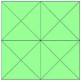
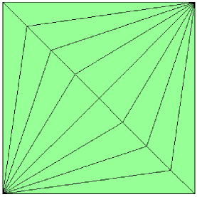
Figure 1. Good and poor quality initial meshes used in the two dimensional examples. The poor quality mesh has a largest angle of approximately $126^{\circ}$ and smallest angle of approximately $8^{\circ}$.

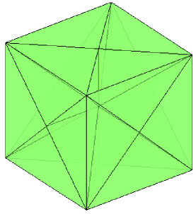
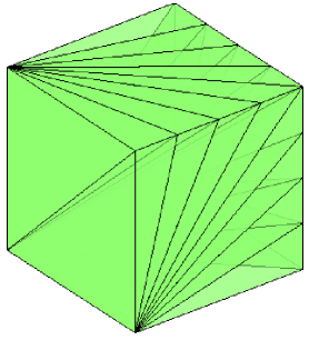
Figure 2. Good and poor quality initial meshes used in the three dimensional examples. The poor quality mesh has a largest dihedral angle of approximately $115^{\circ}$ and smallest dihedral angle of approximately $8^{\circ}$.

Mesh	Worst Quality	Best Quality
Good 2D	0.495	0.693
Poor 2D	0.213	0.283
Good 3D	0.387	0.632
Poor 3D	0.156	0.417

Table 1. Shape Quality Metrics for the various meshes.

Figure 3 and Figure 4 give the convergence results in both $H^{1}$-norm and $L^{\infty}$-norm for the semilinear problems (5.1) in 2D and 3D, respectively. We observe that the quality of the mesh does not ruin the convergence rates in 2D, as long as we keep the mesh to be quasi-uniform. On the other hand, we do observe a little deterioration on the convergence rate in $L^{\infty}$-norm in the 3D example (see Figure 4) when we use a poor quality mesh. However, the errors in $H^{1}$-norm in both 2D and 3D examples seem to be still quasi-optimal as predicted in Theorem 3.2. These results confirm our theoretical conclusions. We also observe that the convergence rate in $L^{\infty}$-norm is close to $h^{2}$ in both the 2D and 3D examples, which indicates that the estimate in (4.15) is not optimal. Even though it is not optimal, we still got the a priori $L^{\infty}$ bound of the discrete solution in (4.16), which is important in the analysis of finite element approximation of nonlinear PDE.

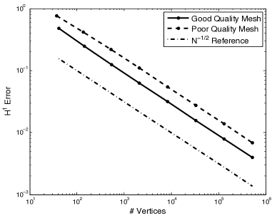
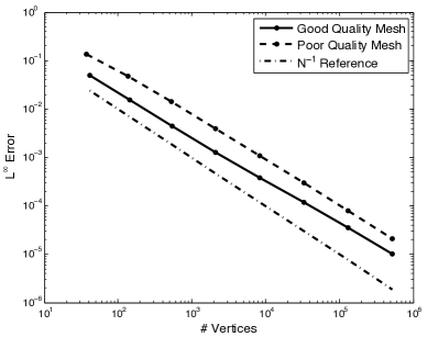
Figure 3. Convergence in $H^{1}$ and $L^{\infty}$ norms for the two-dimensional example problem.

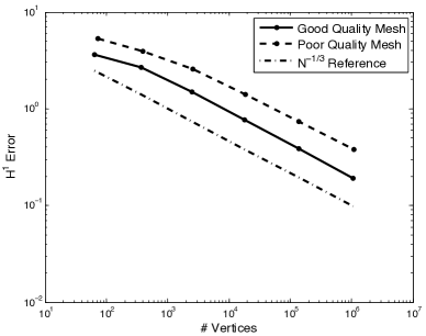
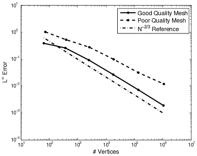
Figure 4. Convergence in $H^{1}$ and $L^{\infty}$ norms for the three-dimensional example problem.

We also run a separate set of experiments in 2D in order to study (4.16) in Corollary 4.4. Specifically, starting with an initial good quality mesh, we compute the discrete solutions on successively worse meshes (produced using shortest edge bisections). Although we do not expect that the discrete solutions converge to the exact solution, we do hope that the $L^{\infty}$ norm of the discrete solution remains bounded. Figure 5 shows the $L^{\infty}$ norm of the discrete solution plotted against the size of the smallest angle in the mesh. This result confirms that the $L^{\infty}$ norm of discrete solutions are uniformly bounded as predicted in Corollary 4.4.

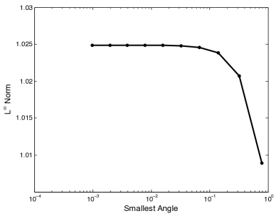
Figure 5. Boundedness of the $L^{\infty}$ norm of the discrete solution computed on successively worse meshes.

6. Conclusion

In this article we considered a priori error estimates for a class of semilinear problems with certain growth condition, which includes problems with critical and subcritical polynomial nonlinearity in $d$ space dimensions. Our motivation was that, while it is well-understood how mesh geometry impacts finite element interpolant quality (at least for $d=2$ and $d=3$). much more restrictive conditions on angles are needed to derive basic a priori quasi-optimal error estimates as well as a priori pointwise estimates for Galerkin approximations. These angle conditions, which are particularly difficult to satisfy in three dimensions in any type of unstructured or adaptive setting, are needed in order to gain pointwise control of the nonlinearity through discrete maximum/minimum principles. Our goal in the article was to show how to derive these types of a priori estimates without requiring the discrete maximum/minimum principles, hence eliminating the need for restrictive angle conditions.

To this end, in Section 2 we described a class of semilinear problems, and reviewed the a priori $L^{\infty}$ bounds of the continuous solution through maximum/minimum principles using the De Giorgi iterative method (or Stampacchia truncation method). We then developed a basic quasi-optimal a priori error estimate for Galerkin approximations in Section 3, where the nonlinearity was controlled by using only a local Lipschitz property rather than through pointwise control of the discrete solution. In this way, we avoid of using discrete maximum principle, which requires certain angle conditions. In particular, we showed that the local Lipschitz property in fact holds for nonlinearities satisfying certain growth condition, which includes the critical exponent cases. We then used some well-known results in finite element approximation theory in Section 4 to show that (under some minimal smoothness assumptions) that the a priori error estimate is itself enough to give $L^{\infty}$ control the discrete solution, without the need for restrictive angle conditions that would be required to obtain a discrete maximum principle.

7. Acknowledgments

MH was supported in part by NSF Awards 0715146 and 0915220, and by DOD/DTRA Award HDTRA-09-1-0036. RB was supported in part by NSF Award 0915220. RS and YZ were supported in part by NSF Award 0715146.

References

- [1] D. Arnold, A. Mukherjee, and L. Pouly. Locally adapted tetrahedral meshes using bisection. SIAM J. Sci. Statist. Comput., 22(2):431–448, 1997.
- [2] T. Aubin. Nonlinear Analysis on Manifolds. Monge-Ampére Equations. Springer-Verlag, New York, NY, 1982.
- [3] I. Babuška and A. K. Aziz. On the angle condition in the finite element method. SIAM Journal on Numerical Analysis, 13(2):214–226, 1976.
- [4] E. Bänsch. Local mesh refinement in 2 and 3 dimensions. Impact of Computing in Science and Engineering, 3:181–191, 1991.
- [5] J. Bey. Tetrahedral grid refinement. Computing, 55(4):355–378, 1995.
- [6] J. H. Bramble, J. A. Nitsche, and A. H. Schatz. Maximum-norm interior estimates for Ritz-Galerkin methods. Mathematics of Computation, 29(131):677–688, 1975.
- [7] C. Budd. Weak finite-dimensional approximations of semi-linear elliptic PDEs with near-critical exponents. Asymptotic Analysis, 17(3):185–220, 1998.
- [8] C. Budd and A. Humphries. Adaptive methods for semi-linear elliptic equations with critical exponents and interior singularities. Applied Numerical Mathematics, 26(1):227–240, 1998.
- [9] L. Chen, M. Holst, and J. Xu. The finite element approximation of the nonlinear Poisson-Boltzmann Equation. SIAM J. Numer. Anal., 45(6):2298–2320, 2007. Available as arXiv:1001.1350 [math.NA].
- [10] M. Chipot. Elliptic equations: an introductory course. Birkhäuser Advanced Texts: Basler Lehrbücher. [Birkhäuser Advanced Texts: Basel Textbooks]. Birkhäuser Verlag, Basel, 2009.
- [11] P. G. Ciarlet. The Finite Element Method for Elliptic Problems, volume 4 of Studies in Mathematics and its Applications. North-Holland Publishing Co., Amsterdam-New York-Oxford, 1978.
- [12] P. G. Ciarlet and P. A. Raviart. Maximum principle and uniform convergence for the finite element method. Computer Methods in Applied Mechanics and Engineering, 2:17–31, 1973.
- [13] E. De Giorgi. Sulla analiticitae la differenziabilita delle estremali degli integrali multipli regolari. Mem. Acc. Sci. Torino, Classe Sci. Fis. Mat. Nat.(3), 3:25–43, 1957.
- [14] A. Demlow. Sharply localized pointwise and estimates for finite element methods for quasilinear problems. Math. Comp., 76:1725–1741, 2007.
- [15] A. Demlow, D. Leykekhman, A. H. Schatz, and L. B. Wahlbin. Best approximation property in the norm on graded meshes. Math. Comp., to appear.
- [16] J. Douglas, T. Dupont, and L. Wahlbin. Optimal error estimates for Galerkin approximation to solutions of two-point boundary value problems. Mathematics of Computation, 29(130):475–483, 1975.
- [17] A. Draganescu, T. F. Dupont, and L. R. Scott. Failure of the discrete maximum principle for an elliptic finite element problem. Mathematics of Computation, 74(249):1–23, 2004.
- [18] S. Fucik and A. Kufner. Nonlinear Differential Equations. Elsevier Scientific Publishing Company, New York, NY, 1980.
- [19] D. Gilbarg and N. S. Trudinger. Elliptic Partial Differential Equations of Second Order. Springer–Verlag, Berlin, New York, 1983.
- [20] M. Holst, J. McCammon, Z. Yu, Y. Zhou, and Y. Zhu. Adaptive finite element modeling techniques for the Poisson-Boltzmann equation. Accepted for Publication in Comm. Comput. Phys. Available as arXiv:1009.6034 [math.NA].
- [21] M. Holst, G. Nagy, and G. Tsogtgerel. Rough solutions of the Einstein constraints on closed manifolds without near-CMC conditions. Comm. Math. Phys., 288(2):547–613, 2009. Available as arXiv:0712.0798 [gr-qc].
- [22] M. Holst, R. Szypowski, G. Tsogtgerel, and Y. Zhu. Convergent adaptive finite element approximation of the Einstein constraints. In preparation.
- [23] M. Holst, R. Szypowski, and Y. Zhu. Two-grid methods for semilinear interface problems. Submitted for publication. Available as arXiv:0000.0000 [math.NA].
- [24] W. Huang. Discrete maximum principle and a Delaunay-type mesh condition for linear finite element approximations of two-dimensional anisotropic diffusion problems. Arxiv preprint arXiv:1008.0562, 2010.
- [25] A. Jüngel and A. Unterreiter. Discrete minimum and maximum principles for finite element approximations of non-monotone elliptic equations. Numer. Math., 99(3):485–508, 2005.
- [26] T. Kerkhoven and J. W. Jerome. stability of finite element approximations of elliptic gradient equations. Numerische Mathematik, 57:561–575, 1990.
- [27] P. M. Knupp. Algebraic mesh quality metrics for unstructured initial meshes. Finite Elem. Anal. Des., 39:217–241, January 2003.
- [28] M. Křížek and J. Pradiova. Nonobtuse tetrahedral partitions. Numerical Methods for Partial Differential Equations, 16(3):327–324, 2000.
- [29] J. Maubach. Local bisection refinement for N-simplicial grids generated by relection. SIAM J. Sci. Statist. Comput., 16(1):210–277, 1995.
- [30] R. H. Nochetto, A. Schmidt, K. G. Siebert, and A. Veeser. Pointwise a posteriori error estimates for monotone semi-linear equations. Numerische Mathematik, V104(4):515–538, 2006.
- [31] A. Quarteroni and A. Valli. Numerical approximation of partial differential equations. Springer, 2008.
- [32] R. Rannacher and R. Scott. Some optimal error estimates for piecewise linear finite element approximations. Mathematics of Computation, 38(158):437–445, 1982.
- [33] V. Santos. On the strong maximum principle for some piece-wise linear finite element approximate problems of non-positive type. Journal of the Faculty of Science, University of Tokyo: Mathematics, 29:473, 1982.
- [34] A. H. Schatz. A weak discrete maximum principle and stability of the finite element method in on plane polygonal domains. I. Math. Comp., 34(149):77–91, 1980.
- [35] A. H. Schatz and L. B. Wahlbin. Interior maximum norm estimates for finite element methods. Mathematics of Computation, 31(138):414–442, 1977.
- [36] A. H. Schatz and L. B. Wahlbin. Maximum norm estimates in the finite element method on plane polygonal domains. I. Math. Comp., 32(141):73–109, 1978.
- [37] A. H. Schatz and L. B. Wahlbin. Interior maximum-norm estimates for finite element methods, part II. Mathematics of Computation, 64(211):907–928, 1995.
- [38] R. Scott. Optimal estimates for the finite element method on irregular meshes. Math. Comp., 30(136):681–697, 1976.
- [39] R. Scott and S. Zhang. Finite element interpolation of nonsmooth functions satisfying boundary conditions. Mathematics of Computation, 54:483–493, 1990.
- [40] I. Stakgold and M. Holst. Green’s Functions and Boundary Value Problems. John Wiley & Sons, Inc., New York, NY, third edition, 888 pages, February 2011. The preface and table of contents of the book are available at: http://ccom.ucsd.edu/~mholst/pubs/dist/StHo2011a-preview.pdf.
- [41] G. Stampacchia. Le probleme de Dirichlet pour les équations elliptiques du second ordrea coefficients discontinus. Ann. Inst. Fourier, 15(1):189–258, 1965.
- [42] G. Strang and G. Fix. An Analysis of the Finite Element Method. Prentice-Hall, Englewood Cliffs, NJ, 1973.
- [43] M. E. Taylor. Partial Differential Equations, volume III. Springer-Verlag, New York, NY, 1996.
- [44] J. Wang and R. Zhang. Maximum principles for -conforming finite element approximations of quasi-linear second order elliptic equations. Arxiv preprint arXiv:1105:1466, 2011.
- [45] Z. Wu, J. Yin, and C. Wang. Elliptic & parabolic equations. World Scientific Publishing Co. Pte. Ltd., Hackensack, NJ, 2006.
- [46] J. Xu. Two-grid discretization techniques for linear and nonlinear PDEs. SIAM Journal on Numerical Analysis, 33(5):1759–1777, 1996.
- [47] J. Xu and A. Zhou. Local and parallel finite element algorithms based on two-grid discretizations. Mathematics of Computation, 231:881–909, 2000.
- [48] J. Xu and A. Zhou. Local and parallel finite element algorithms based on two-grid discretizations for nonlinear problems. Advances in Comp. Math., 14(4):293–327, 2001.