Light-bending tests of Lorentz invariance

Abstract

Classical light bending is investigated for weak gravitational fields in the presence of hypothetical local Lorentz violation. Using an effective field theory framework that describes general deviations from local Lorentz invariance, we derive a modified deflection angle for light passing near a massive body. The results include anisotropic effects not present for spherical sources in General Relativity as well as Weak Equivalence Principle violation. We develop an expression for the relative deflection of two distant stars that can be used to analyze data in past and future solar-system observations. The measurement sensitivities of such tests to coefficients for Lorentz violation are discussed.

I Introduction

A classic prediction of General Relativity (GR) is the bending of distant starlight by the Sun ae . This was first confirmed in 1919 by Dyson, Eddington, and Davidson to agree with Einstein’s calculations of $1.75^{\prime\prime}$ at one Solar radii to within $30\%$ accuracy Dys1920 . More recent optical measurements during solar eclipses have made only marginal improvements optical . The inclusion of radio astronomy has increased the accuracy of light deflection measurements to within $0.02\%$, providing additional firm evidence for the validity of the light deflection predicted in GR vlbi . Measurements of the closely-related Shapiro time delay have also seen vast improvements recently. The analysis of two-way radio tracking of the Cassini probe matched the predictions of GR to within parts in $100,000$ bit .

Although it is currently the best fundamental theory of gravity, there remains widespread interest in developing more precise tests of GR, including improved measurements of the bending of light, among others. These efforts are in part motivated by the intriguing possibility of finding deviations from GR. Such deviations could be a signature of a more fundamental unified theory of physics that successfully meshes GR with quantum theory and the Standard Model of particle physics.

One possible signature that has been sought in many sensitive tests are minuscule violations of local Lorentz invariance, a fundamental tenet of GR reviews . Theoretical scenarios in which local Lorentz symmetry could be broken are currently numerous in the literature, with early motivation coming from string field theory ksp .

In order to investigate violations of local Lorentz invariance, it is useful to have a theoretical framework in which to report measurements. One systematic framework for studying signals of Lorentz violation employs effective field theory. The idea is to incorporate known physics from GR and the Standard Model of particle physics, into an effective action that also includes generic Lorentz-violating terms. The additional Lorentz-violating terms in the action are controlled by coefficients for Lorentz violation, which are general coordinate tensor quantities describing the degree of Lorentz violation for each type of interaction (gravity, electrodynamics, etc.). These coefficients can be thought of as effectively fixed background fields in spacetime that couple to curvature and matter fields, though their origin can be dynamical ksp ; ssb . The framework constructed in this manner is known as the Standard-Model Extension (SME) sme ; akgrav , and has been adopted for numerous tests involving light, matter, and gravity tables . Connections between this framework and various classic test models for Special Relativity are discussed in Refs. km .

Our focus in this work is on the signatures of Lorentz violation for gravitational tests. In the gravity sector of the SME, key signals in a number of experiments and observations have been established in Refs. qbkgrav ; qgrav ; tkgrav ; qgrav2 ; bt10 . Measurements constraining the coefficients for the gravity sector have already begun using atom-interferometric gravimetry atom ; atom2 , lunar laser ranging bcs2007 , and short-range gravity tests bsl2010 . In this paper, we analyze one of the fundamental tests of GR, the bending of light, in the effective field theory framework of the SME. This complements recent work on the related time-delay effect qgrav ; tkgrav .

We begin by deriving a general formula for the deflection angle in section II.1 in terms of an arbitrary post-newtonian metric. The post-newtonian metric is described in Sec. II.2. Assuming a stationary point-like mass we obtain the deflection angle in a limiting case in Sec. II.3, and a more accurate expression in Sec. II.4. In Section III, we apply these results to light-bending tests in the solar system. We develop an expression for the measurable angle between two stars in Sec. III.1. Details of the relative deflection angle and methods of analysis are discussed in Sec. III.2. We illustrate the observable signals for Lorentz violation using a near-conjunction example in Sec. III.3. Finally, in Sec. IV, we summarize the work and estimate the potential measurement sensitivities of existing and future light-bending tests to the coefficients for Lorentz violation in the gravity sector. Throughout this work we adopt notation and conventions as contained in Refs. qbkgrav ; qgrav ; tkgrav . In particular, we work in natural units where $c=1$ and the Minkowski spacetime metric has signature $-+++$.

II Theory

II.1 Deflection basics

The deflection $\vec{\alpha}$ is the shift in the direction that light propagates from a straight line trajectory. We adopt a simplified gravitational lensing or light-bending scenario that involves a source $S$, a mass called the lens $L$, and an observer $O$. The geometric optics limit of electrodynamics in curved spacetime is assumed MTW1973 . For a point-like lens the apparent source position observed by $O$ is $S_{a}$ (see Fig. 1) Wambsganss1998 ; lensing . We assume the lens $L$, the source $S$, and the observer $O$ are stationary throughout the light ray’s propagation. The light ray emission is the event with coordinates $(t_{e},r^{j}_{e})$ and the observation of the light ray has coordinates $(t_{p},r^{j}_{p})$.

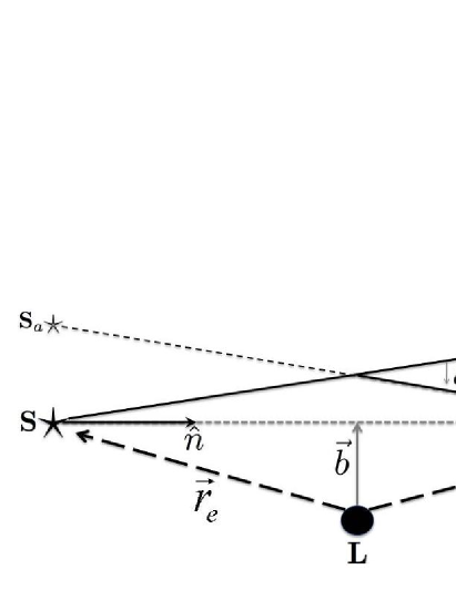
Figure 1: The basic light bending scenario. The vector $\vec{r}_{p}$ extends from the central body $L$ to the observer, $\vec{r}_{e}$ is the vector from the central body to the emitter, $\hat{n}$ is in the direction of the unperturbed path, and $\vec{b}$ is the impact parameter vector (perpendicular to $\hat{n}$).

To calculate the deflection we can exploit Fermat’s principle: the null geodesic path from $(t_{e},r^{j}_{e})$ to the observer’s worldline is equivalent to the extremization of the arrival time $t$ on the observer’s worldline SEF1992 . For a stationary observer, Fermat’s principle is equivalent to the variational principle:

$$\delta\int nd\ell=0.$$ (1)

Here $n$ is the effective index of refraction of the gravitational field, $\ell$ is the euclidean arclength ($d\ell=\sqrt{d\vec{x}^{2}}$), and they are related by $dt=nd\ell$.

The spacetime metric $g_{\mu\nu}$ is expanded around a Minkowski background $\eta_{\mu\nu}$ according to

$$g_{\mu\nu}=\eta_{\mu\nu}+h_{\mu\nu}.$$ (2)

Using the null condition for a light ray ($g_{\mu\nu}dx^{\mu}dx^{\nu}=0$) we can evaluate $n$ to leading order in metric fluctuations $h_{\mu\nu}$ as

$$n\approx 1+{\textstyle{{1}\over{2}}}h_{00}+h_{0j}{{dx^{j}}\over{d\ell}}+{\textstyle{{1}\over{2}}}h_{jk}{{dx^{j}}\over{d\ell}}{{dx^{k}}\over{d\ell}},$$ (3)

where $dx^{j}/d\ell$ is the tangent vector to the light path. The unit vector $\hat{n}^{j}$ is the direction of the zeroth-order tangent to the light path. The light trajectory spatial endpoints are $r^{j}_{e}$ and $r^{j}_{p}$, which correspond to the $\ell$ parameter values $l_{p}$ and $l_{e}$. Referring to Fig. 1, $l_{e}=-\vec{r}_{e}\cdot\hat{n}$ and $l_{p}=\vec{r}_{p}\cdot\hat{n}$. It is useful for later calculations to complete the set $\hat{n}$ and $\hat{b}$ with a perpendicular unit vector called $\hat{\tau}$ defined by $\hat{\tau}=\hat{n}\times\hat{b}$.

If we apply the variational form of Fermat’s principle (1) using the effective index of refraction (3) we obtain equations of motion for the light ray:

$${{d^{2}x^{j}}\over{d\ell^{2}}} \approx \left(\delta^{jk}-{{dx^{j}}\over{d\ell}}{{dx^{k}}\over{d\ell}}\right)$$ (4)

$$\times\left(\partial_{k}n-{{d}\over{d\ell}}\Big{[}h_{0k}+{{dx^{l}}\over{d\ell}}h_{lk}\Big{]}\right).$$

Note that the terms on the right-hand side are perpendicular to $dx^{j}/d\ell$, consistent with the definition of euclidean arclength $\ell$. This equation is equivalent to the geodesic equation for light to post-newtonian order $v^{2}$, or PNO(2).

The deflection $\alpha^{j}$ follows by integration of Eq. (4) from the distant source $S$, at position $r_{e}^{j}$ and $\ell=-l_{e}$, to the observer $O$ at position $r_{p}^{j}$ and $\ell=l_{p}$. To PNO(2), the resulting deflection is given by the expression

$$\alpha^{j}=\int\limits_{-l_{e}}^{l_{p}}(\partial_{j})_{\perp}n\,d\ell-\left[\left(h_{0j}+{{dx^{k}}\over{d\ell}}h_{kj}\right)_{\perp}\right]_{-l_{e}}^{l_{p}},$$ (5)

where the symbol $\perp$ indicates a projection perpendicular to $dx^{j}/d\ell$, as in Eq. (4). The first integral in (5) is evaluated using the Euclidean arclength $d\ell$ along the zeroth-order direction of the light ray. The second term is to be evaluated at the endpoints and plays a role in the result for the case where the observer is near the massive body $L$.

The result in Eq. (5) applies to any metric that can be expanded around a Minkowski background in a post-newtonian series, so long as light behaves conventionally in the geometric optics limit (i.e., light follows a null geodesic). In the sections that follow, we shall apply this result to the post-newtonian metric that incorporates local Lorentz and WEP violations using the SME framework.

II.2 Post-newtonian metric

We focus on the dominant terms in the gravitational sector of the SME framework akgrav . This includes terms augmenting the pure-gravity sector (terms amending the Einstein-Hilbert action) as well as Lorentz-violating terms arising from the matter action. For the case of linearized gravity, the leading corrections to the post-newtonian metric of GR have been established and are discussed in detail in Refs. qbkgrav ; tkgrav . Using a convenient choice of coordinates and existing constraints on the vacuum birefringence of light bire , we can ignore Lorentz violation in the electromagnetic sector, and hence assume light propagates normally tkgrav .

The Lorentz violation for the pure-gravity sector is controlled by $9$ coefficients called $\overline{s}_{\mu\nu}$. For the matter sector, the relevant coefficients are $(\overline{a}_{\rm eff})_{\mu}$ and $\overline{c}_{\mu\nu}$. The combined ${\rm PNO(2)}$ metric in harmonic coordinates is given by

$$g_{00} = -1+\big{[}2+3\overline{s}_{00}+2\overline{c}^{S}_{00}+4{\textstyle{{\alpha}\over{m}}}(\overline{a}_{\rm eff}^{S})_{0}\big{]}U+\overline{s}_{jk}U^{jk},$$

$$g_{0j} = [\overline{s}_{0j}+{\textstyle{{\alpha}\over{m}}}(\overline{a}_{\rm eff}^{S})_{j}]U+[\overline{s}_{0k}+{\textstyle{{\alpha}\over{m}}}(\overline{a}_{\rm eff}^{S})_{k}]U^{jk},$$

$$g_{jk} = \delta_{jk}+[2-\overline{s}_{00}+2\overline{c}^{S}_{00}-2{\textstyle{{\alpha}\over{m}}}(\overline{a}_{\rm eff}^{S})_{0}]\delta_{jk}U$$ (6)

$$+\delta_{jk}\overline{s}_{lm}U^{lm}-\overline{s}_{jl}U^{lk}-\overline{s}_{kl}U^{lj}$$

$$+[2\overline{s}^{00}+2{\textstyle{{\alpha}\over{m}}}(\overline{a}_{\rm eff}^{S})_{0}]U^{jk}.$$

The coefficients for the matter sector, $(\overline{a}_{\rm eff}^{S})_{\mu}$ and $\overline{c}^{S}_{00}$, depend on the structure of the source body $S$ with mass $m$, and therefore will differ for distinct source bodies. Thus $(\overline{a}_{\rm eff}^{S})_{\mu}$ and $\overline{c}^{S}_{00}$ indicate the presence of apparent Weak Equivalence Principle (WEP) violation as well as Lorentz violation. Note, however, that these WEP-violating coefficients do not affect the propagation of light rays, except through the spacetime metric. Also, as discussed in Ref. tkgrav , a model dependent scaling $\alpha$ appears multiplying the coefficients $(\overline{a}_{\rm eff}^{S})_{\mu}$. In contrast, the coefficients $\overline{s}_{\mu\nu}$ do not depend on the nature of the source body and therefore describe WEP-conserving local Lorentz violation for gravity.

Some limiting cases of this metric should be noted. This post-newtonian metric can be viewed as enlarging and complementing the Parametrized Post-Newtonian (PPN) metric Will2006 as discussed, for the case of vanishing matter coefficients, in Ref. qbkgrav . Also, in the limit that the coefficients $\overline{s}_{\mu\nu}$, $(\overline{a}_{\rm eff}^{S})_{\mu}$, and $\overline{c}^{S}_{00}$ vanish, this result reduces to the post-Newtonian metric of GR.

For classical light bending scenarios we assume the source body $L$ to be a point-like mass $M$. Furthermore, the source body is taken as the origin of the coordinate system. Thus, the dominant contributions to the potentials $U$ and $U^{jk}$ depend on the position of the test body $r^{j}$:

$$U = {{GM}\over{r}},$$ (7)

$$U^{jk} = {{GMr^{j}r^{k}}\over{r^{3}}},$$ (8)

where $G$ is Newton’s gravitational constant.

II.3 Light deflection: grazing case

As a preliminary investigation of the modifications to the standard GR light-bending formula, we consider the simplified “grazing” case. In this scenario both the emitter and receiver are assumed to be very far from the source, thus we take $l_{p}\rightarrow\infty$ and $l_{e}\rightarrow\infty$. Using the metric (6) in the general result (5) we obtain for this limiting case the deflection

$$\alpha^{j} = {{-4GM}\over{b}}\Big{(}[1+\overline{s}_{00}+\overline{c}^{S}_{00}+{\textstyle{{\alpha}\over{M}}}(\overline{a}_{\rm eff}^{S})_{0}$$

$$\phantom{{{4GM}\over{b}}}+(\overline{s}_{0k}+{\textstyle{{\alpha}\over{M}}}(\overline{a}_{\rm eff}^{S})_{k})\hat{n}^{k}]\hat{b}^{j}-\overline{s}_{kl}\hat{b}^{k}\hat{\tau}^{l}\hat{\tau}^{j}\Big{)}.$$

The standard GR result is obtained in the limit that the coefficients for Lorentz violation vanish.

To illustrate some of the features of the result (LABEL:defl:2) we employ vector field plots indicating the apparent shift of incoming starlight as the source appears in front of a background of initially uniformly distributed stars. This is similar to methods that have been adopted for the GR signal in Refs. cm ; kop06 . For this simulation we focus on a small patch of sky centered on the deflecting body. We use $x$ and $y$ coordinates on the patch to make a vector field plot of different parts of the result (LABEL:defl:2). These coordinates will lie in the plane perpendicular to the unit vector $\hat{n}$, which we can take to point (approximately) from the deflecting body to the observer.

The left panel of Fig. 3 shows the initial star field in the absence of the source. For simplicity, we assume the distribution of stars is uniform. The right panel of Fig. 3 shows the deflection in the GR limit. In the expression for the deflection (LABEL:defl:2), the term proportional to $\hat{b}^{j}$ is scaled by the coefficients for Lorentz violation $\overline{s}_{00}+\overline{c}^{S}_{00}+(\alpha/M)(\overline{a}_{\rm eff}^{S})_{0}$ and the $\hat{n}$-dependent combination $(\overline{s}_{0k}+(\alpha/M)(\overline{a}_{\rm eff}^{S})_{k})\hat{n}^{k}$. Note that, due to the appearance of these coefficients, this scaling will change depending on the location of the patch of sky considered and the internal nature of the source. That this occurs is due to the anisotropy of the coefficients for Lorentz violation and their composition dependence.

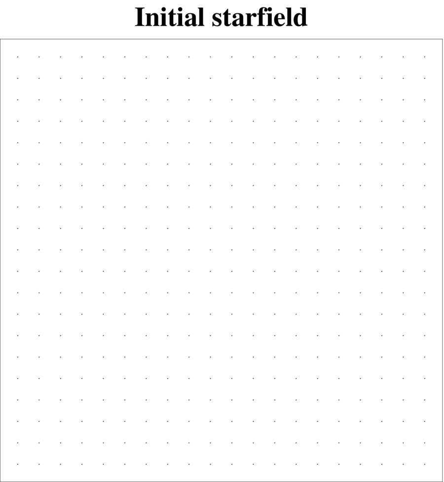
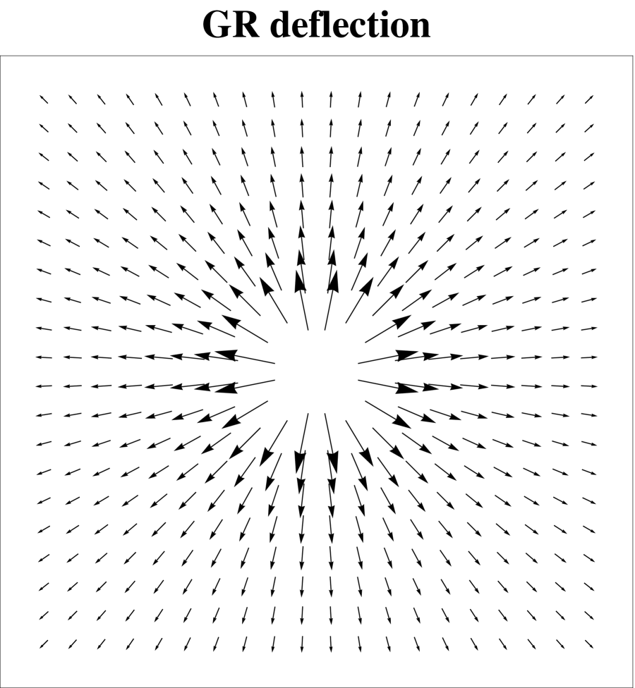
Figure 2: Initial uniform star field (left). Apparent shift of distant light in the standard general relativity case (right).

Figure 3: Anisotropic apparent shift of star field due to the $\overline{s}_{xx}-\overline{s}_{yy}$ coefficients (left) and the $\overline{s}_{xy}$ coefficients (right). The local $x$ coordinate runs horizontally and $y$ is vertical.

The last term in Eq. (LABEL:defl:2) points in the direction $\hat{\tau}$, orthogonal to $\hat{b}$. This term is proportional to the combination of coefficients $\overline{s}_{kl}\hat{b}^{k}\hat{\tau}^{l}$. If we express this combination in terms of the ($x$, $y$) coordinates on the patch of sky considered, this can be expanded into the two independent combinations $\overline{s}_{\,xx}-\overline{s}_{\,yy}$ and $\overline{s}_{\,xy}$. The deflections due to these two combinations of coefficients are plotted in Fig. 3, where we have set their values to one for illustration. These plots indicate that anisotropic deflection occurs for nonvanishing coefficients $\overline{s}_{jk}$. In particular, this means that a light ray would deflect off of an otherwise flat plane defined by $\hat{n}$ and $\hat{b}$, contrary to the conventional GR point-mass case. Note that these anisotropic effects can in principle be distinguished from the GR deflection due to higher multipole moments of the deflecting body zk ; kop06 by virtue of their $1/b$ dependence.

It is interesting to compare this result with that obtained in Refs.  qgrav ; tkgrav for the gravitational time delay in the presence of local Lorentz violation. The vector coefficients $\overline{s}_{0j}$ and $(\alpha/M)(\overline{a}_{\rm eff}^{S})_{j}$ appear in the light bending result (LABEL:defl:2), while they are absent in the round-trip time delay signal. Also, light-bending observations that involve one orientation of the observer, deflecting body, and the distant starlight could gain access to sets of coefficients distinct from those in a dedicated time-delay test with a different orientation of the relevant bodies. Note that this feature does not occur in the PPN formalism, for which both types of tests access the same parameter regardless of the underlying orientation.

II.4 Light deflection: general case

For applications of (5) to observations, the light-grazing approximation previously assumed must be reconsidered. Here we still assume $l_{e}\rightarrow\infty$, but $l_{p}$ is treated as a relevant, finite term. This corresponds to the case where the observer is a finite distance from the lens $L$, while the light source is effectively at spatial infinity. Referring to Fig. 1 it will be useful to define an angle $\Phi$ between $\vec{r}_{p}$ and $\hat{n}$ (thus $\hat{r}_{p}\cdot\hat{n}=\cos\Phi$).

Evaluating the deflection formula (5) using the metric (6) for the case $l_{e}\rightarrow\infty$, we obtain the deflection,

$$\alpha^{j} = {{-GM}\over{b}}\Bigg{[}\hat{b}^{j}\bigg{(}2(1+\overline{s}_{00}+\overline{c}^{S}_{00}+{\textstyle{{\alpha}\over{M}}}(\overline{a}_{\rm eff}^{S})_{0}$$

$$\phantom{+}+(\overline{s}_{0k}+{\textstyle{{\alpha}\over{M}}}(\overline{a}_{\rm eff}^{S})_{k})\hat{n}^{k})(1+\cos\Phi)$$

$$\phantom{+}+(\overline{s}_{00}+{\textstyle{{\alpha}\over{M}}}(\overline{a}_{\rm eff}^{S})_{0}-\overline{s}_{kl}\hat{n}^{k}\hat{n}^{l})\cos\Phi\sin^{2}\Phi$$

$$\phantom{+}+2(\overline{s}_{0k}+{\textstyle{{\alpha}\over{M}}}(\overline{a}_{\rm eff}^{S})_{k})\hat{b}^{k}\sin\Phi-\overline{s}_{kl}\hat{n}^{k}\hat{b}^{l}\sin^{3}\Phi\bigg{)}$$

$$+\hat{\tau}^{j}\bigg{(}2(\overline{s}_{0k}+{\textstyle{{\alpha}\over{M}}}(\overline{a}_{\rm eff}^{S})_{k})\hat{\tau}^{k}\sin\Phi+\overline{s}_{kl}\hat{n}^{k}\hat{\tau}^{l}\sin^{3}\Phi$$

$$\phantom{+\tau^{j}(}-\overline{s}_{kl}\hat{b}^{k}\hat{\tau}^{l}(2+2\cos\Phi+\cos\Phi\sin^{2}\Phi)\bigg{)}\Bigg{]}$$

(10)

where the substitutions of $l_{p}/r_{p}=\cos\Phi$ and $b/r_{p}=\sin\Phi$ have been made. Note that in the light-grazing limit the $\sin\Phi$ term vanishes and the $\cos\Phi$ term approaches unity, which results in the previous deflection angle presented in (LABEL:defl:2).

The result (10) indicates that additional projections of coefficients for Lorentz violation arise in the more accurate deflection formula. Also, these additional combinations of coefficients appear to be distinct from the those that occur in the gravitational time delay derived in Refs. qgrav ; tkgrav . By itself, the deflection in Eq. (10) is not directly measurable. This is because only the apparent position of a given source star is actually measured (at least during a single observation period). Instead, a comparative measurement is needed based on two or more observations. In the following section we apply this result to calculate the relative deflection of two stars, which is a measurable quantity.

III Solar System Tests

The key observable of interest for typical light bending measurements is the relative deflection of two (or more) stars. We seek here the angle between a “source” star and a “reference” star. In what follows quantities associated with the reference star will have $r$ subscripts, and those for the source star will have no subscripts. The apparent positions of both of these stars will in principle be gravitationally deflected if the lens is near the line of sight. By continuous monitoring of the relative position of these two stars, one can measure the effects of the deflection (10). Furthermore, the formula we derive below can in principle be applied repeatedly to systems of many stars.

III.1 Relative deflection

To calculate the relative deflection we adopt standard methods in the literature Will2006 ; gaia2 . We begin with a general coordinate invariant expression for the angle $\Psi$ between two stars:

$$\cos\Psi=1+{{p^{\mu}(p_{r})_{\mu}}\over{(u^{\nu}p_{\nu})(u^{\lambda}(p_{r})_{\lambda})}}.$$ (11)

In this expression $p^{\mu}$ and $(p_{r})^{\mu}$ are the tangent four-vectors for the source light ray and the reference light ray, respectively. The four-velocity of the observer measuring the relative angle is $u^{\mu}$. Evaluating this expression to ${\rm PNO(2)}$, and neglecting aberration terms, we obtain

$$\cos\Psi=\hat{n}\cdot\hat{n}_{r}+\hat{n}\cdot(\vec{\alpha}_{\rm eff})_{r}+\hat{n}_{r}\cdot\vec{\alpha}_{\rm eff},$$ (12)

where $\vec{\alpha}_{\rm eff}$ is given by

$$\alpha_{\rm eff}^{j}=\alpha^{j}+{\textstyle{{1}\over{2}}}(\hat{n}^{k}h_{kj})_{\perp}|_{\ell=\ell_{p}}.$$ (13)

The deflection $\alpha^{j}$ is obtained from Eq. (10) and quantities with the label $r$ are obtained by re-labeling all quantities occurring in the expression, involving the direction of the light ray, with the subscript $r$ (e.g., $\hat{n}\rightarrow\hat{n}_{r}$, $\hat{b}\rightarrow\hat{b}_{r}$, etc. ). The zeroth order, or straight line, trajectories from the source and reference stars are depicted in Fig. 4.

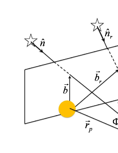
Figure 4: Solar light-bending scenario in the presence of a reference source. For the source and reference star, we have the impact parameters $\vec{b}$ and $\vec{b}_{r}$, and directions $\hat{n}$ and $\hat{n}_{r}$, respectively. The reference plane shown is that spanned by $\vec{b}$ and $\vec{b}_{r}$.

We define an angle $\Psi_{0}$ that represents the unperturbed angle between the two stars:

$$\hat{n}_{r}\cdot\hat{n}=\cos\Psi_{0}$$ (14)

Thus $\Psi_{0}$ is the angle between the two stars in flat spacetime in the absence of other conventional effects such as aberration. The shift or change in the angle between the two stars is defined to be

$$\delta\Psi=\Psi-\Psi_{0}.$$ (15)

Since we are working in the post-newtonian approximation it suffices to assume $\delta\Psi$ is small so that $\cos\Psi\approx\cos\Psi_{0}-\delta\Psi\sin\Psi_{0}$. Using this approximation, the previous result (10), and the metric in (6), we obtain

$$\sin\Psi_{0}\delta\Psi \approx {{GM}\over{b}}\left(\hat{n}_{r}\cdot\hat{b}[2(1+\cos\Phi)+B]+\hat{n}_{r}\cdot\hat{\tau}T\right)$$

$$\hskip-10.0pt+{{GM}\over{b_{r}}}\left(\hat{n}\cdot\hat{b}_{r}[2(1+\cos\Phi_{r})+B_{r}]+\hat{n}\cdot\hat{\tau}_{r}T_{r}\right)$$

In (LABEL:delps:2) the terms $B$, $T$, $B_{r}$ and $T_{r}$ are proportional to combinations of the coefficients for Lorentz violation $\overline{s}_{\mu\nu}$, $\overline{c}^{S}_{00}$, and $(\overline{a}_{\rm eff}^{S})_{\mu}$. Explicitly, they are given by

$$B = 2[\overline{s}_{00}+\overline{c}^{S}_{00}+{\textstyle{{\alpha}\over{M}}}(\overline{a}_{\rm eff}^{S})_{0}$$ (17)

$$\phantom{2}+(\overline{s}_{0k}+{\textstyle{{\alpha}\over{M}}}(\overline{a}_{\rm eff}^{S})_{k})\hat{n}^{k}](1+\cos\Phi)$$

$$+{\textstyle{{1}\over{2}}}(\overline{s}_{kl}\hat{b}^{k}\hat{b}^{l}-\overline{s}_{kl}\hat{n}^{k}\hat{n}^{l})\cos\Phi\sin^{2}\Phi$$

$$+2(\overline{s}_{0k}+{\textstyle{{\alpha}\over{M}}}(\overline{a}_{\rm eff}^{S})_{k})\hat{b}^{k}\sin\Phi$$

$$\phantom{2}-\overline{s}_{kl}\hat{n}^{k}\hat{b}^{l}\sin\Phi(\sin^{2}\Phi-{\textstyle{{1}\over{2}}})$$

$$B_{r} = 2[\overline{s}_{00}+\overline{c}^{S}_{00}+{\textstyle{{\alpha}\over{M}}}(\overline{a}_{\rm eff}^{S})_{0}$$ (18)

$$\phantom{2}+(\overline{s}_{0k}+{\textstyle{{\alpha}\over{M}}}(\overline{a}_{\rm eff}^{S})_{k})\hat{n}_{r}^{k}](1+\cos\Phi_{r})$$

$$+{\textstyle{{1}\over{2}}}(\overline{s}_{kl}\hat{b}_{r}^{k}\hat{b}_{r}^{l}-\overline{s}_{kl}\hat{n}_{r}^{k}\hat{n}_{r}^{l})\cos\Phi_{r}\sin^{2}\Phi_{r}$$

$$+2(\overline{s}_{0k}+{\textstyle{{\alpha}\over{M}}}(\overline{a}_{\rm eff}^{S})_{k})\hat{b}_{r}^{k}\sin\Phi_{r}$$

$$\phantom{2}-\overline{s}_{kl}\hat{n}_{r}^{k}\hat{b}_{r}^{l}\sin\Phi_{r}(\sin^{2}\Phi_{r}-{\textstyle{{1}\over{2}}})$$

$$T = 2(\overline{s}_{0k}+{\textstyle{{\alpha}\over{M}}}(\overline{a}_{\rm eff}^{S})_{k})\hat{\tau}^{k}\sin\Phi$$ (19)

$$+{\textstyle{{1}\over{2}}}\overline{s}_{kl}\hat{n}^{k}\hat{\tau}^{l}\sin\Phi(1+\sin^{2}\Phi)$$

$$-\overline{s}_{kl}\hat{b}^{k}\hat{\tau}^{l}(2+2\cos\Phi+{\textstyle{{1}\over{2}}}\cos\Phi\sin^{2}\Phi)$$

$$T_{r} = 2(\overline{s}_{0k}+{\textstyle{{\alpha}\over{M}}}(\overline{a}_{\rm eff}^{S})_{k})\hat{\tau}_{r}^{k}\sin\Phi_{r}$$ (20)

$$+{\textstyle{{1}\over{2}}}\overline{s}_{kl}\hat{n}_{r}^{k}\hat{\tau}_{r}^{l}\sin\Phi_{r}(1+\sin^{2}\Phi_{r})$$

$$-\overline{s}_{kl}\hat{b}_{r}^{k}\hat{\tau}_{r}^{l}(2+2\cos\Phi_{r}+{\textstyle{{1}\over{2}}}\cos\Phi_{r}\sin^{2}\Phi_{r})$$

The usual result from general relativity is obtained for vanishing coefficients for Lorentz violation, which follows here in the limit $B=T=B_{r}=T_{r}=0$.

The result in Eq. (LABEL:delps:2) exhibits several interesting features that do not occur in the point-mass limit of GR. First, the rotational scalar combinations involving $\overline{s}_{00}$, $\overline{c}^{S}_{00}$, and $(\overline{a}_{\rm eff}^{S})_{0}$ scale the usual GR result. However, due to the composition dependence of $\overline{c}^{S}_{00}$ and $(\overline{a}_{\rm eff}^{S})_{0}$, this scaling will vary with the central body (or Lens) producing the gravitational deflection. Secondly, the anisotropic coefficients $\overline{s}_{0j}$, $(\overline{a}_{\rm eff}^{S})_{j}$, and $\overline{s}_{jk}$ occur in the deflection result such that they are projected along directions associated with the position of the source and reference star ($\hat{n}$, $\hat{n}_{r}$, etc.). This implies that observations made either with significantly changing star positions, or made with different sets of stars at different locations in the sky, will experience different deflections. This effect is independent of the conventional $\Phi$, $\Phi_{r}$, and $\Psi_{0}$ dependence of the deflection. Thirdly, deflection occurs in the directions $\hat{\tau}$ and $\hat{\tau}_{r}$ perpendicular to $\hat{n}$ and $\hat{n}_{r}$, as already illustrated in Figs. 3. The anisotropic effects imply that observations made over time or with many stars would yield access to different combinations of coefficients for Lorentz violation, thus increasing the potential “parameter space” of possible types of Lorentz violations to which light deflection observations could be sensitive.

III.2 Observational analysis

The form of Eq. (LABEL:delps:2) indicates that it depends on a number of parameters which can be related to specific measurable astronomical quantities, in addition to its dependence on coefficients for Lorentz violation. To illustrate this we describe in this section how analysis might proceed. Our post-newtonian coordinate system is taken to coincide with the standard Sun-centered celestial equatorial coordinate system adopted for many studies of Lorentz violation. The spatial coordinates are denoted by $X$, $Y$, and $Z$ with $X$ pointing in the direction of the Sun at the vernal equinox, and $Z$ is aligned with the Earth’s rotation axis. The time coordinate is $T$ and is typically defined so that $T=0$ at the $2000$ vernal equinox. Details of the Sun-centered celestial equatorial coordinate system can be found in Refs. scf ; tables . In particular, the reader is referred to a depiction of this coordinate system in Fig. $1$ of Ref. tables .

In general, for data analysis, one can seek to express the relative deflection (LABEL:delps:2) such that its functional form is

$$\delta\Psi=\delta\Psi(\theta,\theta_{r},\phi,\phi_{r},T,\overline{s}_{\mu\nu},(\overline{a}_{\rm eff}^{S})_{\mu},\overline{c}^{S}_{TT},...).$$ (21)

The first four parameters $(\theta,\phi)$ and $(\theta_{r},\phi_{r})$ determine, respectively, the direction of $\hat{n}$ and $\hat{n}_{r}$ relative to the Sun-centered frame. Explicitly, the unit vectors take the form

$$\hat{n} = -(\sin\theta\cos\phi,\sin\theta\sin\phi,\cos\theta),$$

$$\hat{n}_{r} = -(\sin\theta_{r}\cos\phi_{r},\sin\theta_{r}\sin\phi_{r},\cos\theta_{r}).$$ (22)

Specifically, ($\theta$, $\phi$) and ($\theta_{r}$, $\phi_{r}$) are taken as co-latitude and right ascension on the celestial sphere for the source star and reference star, respectively. In terms of these angles, the angle $\Psi_{0}$ can be determined using Eq. (14) and the angles $\Phi$ can $\Phi_{r}$ can be determined using $\hat{r}_{p}\cdot\hat{n}=\cos\Phi$ and $\hat{r}_{p}\cdot\hat{n}_{r}=\cos\Phi_{r}$.

The time parameter $T$ appears in part due to the observer’s motion in the Sun-centered frame. To sufficient accuracy in any of the Lorentz-violating terms of (21) we can assume that the motion of the observer is explicitly known. For example, for the Earth we can assume a circular orbit and use

$$\hat{r}_{p}=(-\cos\Omega T,-\cos\eta\sin\Omega T,-\sin\eta\sin\Omega T),$$ (23)

where $\eta$ is the inclination of the ecliptic to the equatorial plane and $\Omega$ is the Earth’s orbital frequency.

The last set of parameters $\overline{s}_{\mu\nu}$, $(\overline{a}_{\rm eff}^{S})_{\mu}$, and $\overline{c}^{S}_{TT}$ are the coefficients for Lorentz violation expressed in the Sun-centered frame coordinates. In addition to the dot products ($\hat{n}_{r}\cdot\hat{b}$, $\hat{n}_{r}\cdot\hat{\tau}$, etc.), the terms occurring in the deflection formula (LABEL:delps:2) contain projections of the coefficients along the six unit vectors for the source and reference source $\{\hat{n},\hat{b},\hat{\tau},\hat{n}_{r},\hat{b}_{r},\hat{\tau}_{r}\}$. To capture the orientation dependence of the coefficients we must express all of these unit vectors in the Sun-centered frame. This can be accomplished using (22) and (23). The impact parameter vector is defined by $\vec{b}=\vec{r}_{p}-\hat{n}(\hat{n}\cdot\vec{r}_{p})$ (see Fig. 1). Using this, the unit vectors $\hat{b}$ and $\hat{b}_{r}$ can be written as

$$\hat{b} = {{\hat{r}_{p}-\hat{n}\cos\Phi}\over{\sin\Phi}},$$

$$\hat{b}_{r} = {{\hat{r}_{p}-\hat{n}_{r}\cos\Phi_{r}}\over{\sin\Phi_{r}}}.$$ (24)

From this expression and (22) the unit vectors $\hat{\tau}$ and $\hat{\tau}_{r}$ can be constructed using the cross products

$$\hat{\tau} = \hat{n}\times\hat{b},$$

$$\hat{\tau}_{r} = \hat{n}_{r}\times\hat{b}_{r}.$$ (25)

The full set of unit vectors allows us to express projections of the coefficients in terms of Sun-centered frame quantities. For example, if only $\overline{s}_{XZ}$ happens to be nonzero, we obtain for the projection $\overline{s}_{JK}\hat{\tau}^{J}\hat{b}^{K}$,

$$\overline{s}_{JK}\hat{\tau}^{J}\hat{b}^{K} = \overline{s}_{XZ}(\hat{\tau}^{X}\hat{b}^{Z}+\hat{\tau}^{Z}\hat{b}^{X})$$ (26)

$$= \csc^{2}\Phi\overline{s}_{XZ}[\sin\theta$$

$$\times(\sin\phi\cos\Omega T-\cos\eta\cos\phi\sin\Omega T)$$

$$\times(\cos\Omega T-\sin\theta\cos\Phi\cos\phi)$$

$$+\sin\Omega T(\sin\eta\sin\theta\sin\phi-\cos\eta\cos\theta)$$

$$\times(\cos\theta\cos\Phi-\sin\eta\sin\Omega T)],$$

where we assumed the case of an Earth observer and made use of the formula (23) for $\hat{r}_{p}$.

The full expression of the deflection angle (LABEL:delps:2), in terms of the parameters indicated in (21), can be obtained using the methods just described. This calculation is lengthy, and so we do not include it here, but it should be straightforward to include in a suitable data analysis code. To give a flavor of the leading Lorentz-violating effects in light bending, we determine the approximate form of (LABEL:delps:2) for a special case in the next subsection.

Finally we note that we have included ellipses in expression (21) to indicate that we have not discussed a number of other astronomical parameters that may be important to a rigorous analysis, such as the effects of parallax and proper motion. Furthermore, we have neglected aberration effects in the result (LABEL:delps:2) that depend on the Earth’s or observer’s velocity. We find that one effect of these terms is that they multiply the coefficients for Lorentz violation in (LABEL:delps:2) by higher powers of velocity, resulting in ${\rm PNO(3)}$ effects. In addition, terms proportional to $\vec{v}$ or its square that arise for aberration in the conventional case soffel , can implicitly depend on the coefficients for Lorentz violation through orbital dynamics. The effects of Lorentz violation on orbits can in principle be incorporated using the equations of motion derived in Refs. qbkgrav ; tkgrav .

III.3 Conjunction example

To elucidate the Lorentz-violating effects in the main result (LABEL:delps:2), we work with a special case of the general SME deflection result that involves only one set of coefficients for Lorentz violation. We set to zero all coefficients save those contained in $\overline{s}_{JK}$. We also ignore any contributions from $\overline{s}_{JJ}=\overline{s}_{TT}$ that scale the GR deflection.

We focus in this example on an Earth observer during times near the summer solstice when the Earth lies below the negative $Y$ axis in the Sun-centered frame (the summer solstice occurs when $\Omega T=\pi/2$). To exploit the peak behavior of the deflection result (LABEL:delps:2), we suppose that the source star is located on the celestial sphere so that its light just grazes the Sun on its way to earth. The reference star is taken to be a considerable angular distance away from the source star so that its gravitational deflection can be ignored to a good approximation. For simplicity, both stars are assumed to have $\phi=\pi/2=\phi_{r}$.

In this near-conjunction scenario, the formula for the unit vector in the direction of the Earth observer is given by (23) while the unit vector for the source star is given by

$$\hat{n}=-(0,\cos(\eta+\epsilon),\sin(\eta+\epsilon)),$$ (27)

where $\epsilon$ is a small angle indicative of the near-conjunction approximation adopted. The other needed unit vectors $\hat{b}$ and $\hat{\tau}$ can be obtained from the results in the previous subsection.

If we focus on only the dominant terms in this scenario, the result (LABEL:delps:2) simplifies considerably. As previously stated, the second term in (LABEL:delps:2) proportional to $GM/b_{r}$ that involves the reference star quantities can be neglected since $b<<b_{r}$. We can also discard any terms with one or more powers of $\sin\Phi$, since they will be suppressed in this limit. Finally, using the small angle approximation for $\epsilon$ can further simplify the expression.

If $t$ is the time measured from the summer solstice, the GR portion of the deflection becomes

$$\delta\Psi_{\rm GR}\approx-2{{GM_{\odot}}\over{R}}{{\sin\epsilon}\over{(1-\cos\Omega t\cos\epsilon)}}$$ (28)

where $R$ is the earth’s orbital radius and $M_{\odot}$ is the Sun’s mass. The portion of the deflection controlled by the coefficients for Lorentz violation $\overline{s}_{JK}$ stems from the $\overline{s}_{JK}\hat{\tau}^{J}\hat{b}^{K}$ term in Eq. (LABEL:delps:2). It is given by

$$\delta\Psi_{\rm LV} \approx -{{GM_{\odot}}\over{R}}{{\sin\Omega t}\over{(1-\cos\Omega t\cos\epsilon)^{2}}}$$ (29)

$$\times(\overline{s}_{A}\sin\Omega t\cos\Omega t\sin\epsilon$$

$$\phantom{space}+\overline{s}_{B}[\cos^{2}\Omega t\sin^{2}\epsilon-\sin^{2}\Omega t]),$$

where the combinations of coefficients $\overline{s}_{A}$ and $\overline{s}_{B}$ are given by

$$\overline{s}_{A} = \sin^{2}\eta\overline{s}_{YY}+\cos^{2}\eta\overline{s}_{ZZ}-\overline{s}_{XX}-\sin 2\eta\overline{s}_{YZ},$$

$$\overline{s}_{B} = \sin\eta\overline{s}_{XY}-\cos\eta\overline{s}_{XZ}.$$ (30)

The result from GR in (28) is plotted in Fig. 5 near the time of conjunction ($t=0$) using the values $\eta=23.4^{\circ}$ and $\epsilon=0.27^{\circ}$ (grazing limit). This deflection is peaked and is symmetrical around $t=0$. For the Sun as the deflecting body, the peak value of $1.75"$ is well known. Note that the sign of the GR deflection is negative. This is consistent with the (outward) apparent deflection depicted in Fig. 3, since $\delta\Psi_{\rm GR}=\Psi-\Psi_{0}$ is the difference in the observed angle from the unperturbed, or zeroth-order angle.

Figure 5: The behavior of the deflection $\delta\Psi$ near conjunction plotted as function of time $t$ around the summer solstice as the Sun moves across the field of view. The solid curve is the deflection from GR, the dashed curve is the deflection amplitude from the coefficients $\overline{s}_{A}$, and the dotted curve is the deflection amplitude from the coefficients $\overline{s}_{B}$.

The two types of Lorentz-violating signals in (29) are also plotted in Fig. 5 near the time of conjunction using the same assumptions on $\eta$ and $\epsilon$. For these curves we plot amplitudes, or “partials”, for each of the coefficient combinations $\overline{s}_{A}$ and $\overline{s}_{B}$. It is evident that these signals are qualitatively different from the GR case. The amplitude for $\overline{s}_{A}$ displays symmetrical behavior around $t=0$ while the amplitude for $\overline{s}_{B}$ is antisymmetric around $t=0$. Both of these signals display mildly oscillatory behavior near $t=0$ that could potentially be useful for analysis.

If measurements were obtained for differing orientations of the observer, the signals for Lorentz violation would involve coefficient combinations distinct from those in Eq. (30). As an example of this orientation dependence, suppose instead that the (near-conjunction) observations took place with the Earth near the vernal equinox, when the Sun is along the positive $X$ axis of the chosen coordinate system. The GR result is very similar to Eq. (28) in this case, but the Lorentz-violating piece $\delta\Psi_{\rm LV}$ differs in its details. Specifically, for this configuration we find

$$\delta\Psi_{\rm LV} \approx {{GM_{\odot}}\over{R}}{{\cos\eta\sin\Omega T}\over{(1-\cos\Omega T\cos\epsilon-\sin\eta\sin\epsilon\sin\Omega T)^{2}}}$$ (31)

$$\times[(\overline{s}_{YY}-\overline{s}_{ZZ})({\textstyle{{1}\over{2}}}\sin 2\eta\sin^{2}\Omega T$$

$$\phantom{\times\,\overline{s}_{YY}-\overline{s}_{ZZ}}-\cos\eta\sin\Omega T\cos\Omega T\sin\epsilon)$$

$$+\overline{s}_{YZ}(\cos^{2}\Omega T\sin^{2}\epsilon-\cos 2\eta\sin^{2}\Omega T$$

$$\phantom{space}-2\sin\eta\sin\epsilon\sin\Omega T\cos\Omega T)],$$

where $T$ is measured from the conjunction time $T=0$. It is evident from this result that the signal depends on the coefficients combinations $\overline{s}_{YY}-\overline{s}_{ZZ}$ and $\overline{s}_{YZ}$, rather than those given in Eqs. (30).

IV Summary and estimates

In this work we have identified the dominant signals for local Lorentz violation in light-bending observations. A general formula making use of euclidean arclength that is valid for the post-newtonian limit of any stationary metric was established in (5). Working within the SME effective field theory framework, we applied this formula to the deflection of a light ray from a straight line path in the grazing limit in Eq. (LABEL:defl:2), and more accurately in Eq. (10). The results display anisotropic behavior of light bending controlled by coefficients for Lorentz violation, as demonstrated in Fig. 3.

In the latter part of this work, we calculate a more practical formula for the change in the measured angle $\Psi$ between two stars in Eq. (LABEL:delps:2). We describe generally how this result can be expressed in terms of astronomical quantities suitable for data analysis. The approximate behavior of the deflection angle shift $\delta\Psi$ on the coefficients for Lorentz violation was elucidated with a specific near-conjunction example. We compare this unconventional behavior with the standard behavior predicted from GR (see Fig. 5).

It would be of interest to perform a rigorous analysis of potential sensitivities for future missions, perhaps involving detailed simulations. Such simulations have already been performed for the GR and PPN case for the planned Gaia mission gaia2 ; gaia3 . The starting point for such simulations is typically the relative deflection between two stars. We provide this expression for the SME in Eqs. (12) and (LABEL:delps:2) of this work. A numerical least squares estimation could be attempted using the partial derivatives of $\Psi$ with respect to the coefficients for Lorentz violation $\overline{s}_{\mu\nu}$, $(\overline{a}_{\rm eff}^{S})_{\mu}$, and $\overline{c}^{S}_{00}$, along with other relevant parameters.

Observatory	$\overline{s}^{\prime}_{TT}$	$\overline{s}_{TJ}+(\alpha/M)(\overline{a}_{\rm eff}^{S})_{J}$	$\overline{s}_{JK}$	Ref.
LATOR	$10^{-8}$	$10^{-8}$	$10^{-7}$	lator
Gaia	$10^{-6}$	$10^{-6}$	$10^{-5}$	gaia2
Hipparcos	$10^{-3}$	$10^{-3}$	$10^{-2}$	hipp
Optical	$10^{-1}$	$1$	$1$	optical

Table 1: Crude estimates of sensitivities of current and future light-bending tests to various combinations of coefficients for Lorentz violation. The shorthand $\overline{s}^{\prime}_{TT}$ is defined by $\overline{s}^{\prime}_{TT}=\overline{s}_{TT}+\overline{c}^{S}_{TT}+{\textstyle{{\alpha}\over{M}}}(\overline{a}_{\rm eff}^{S})_{T}$.

Though it is beyond the scope of this work to perform detailed simulations for future missions or analysis of available data from current and past observations, we provide in Table 1 order of magnitude estimates of sensitivities to different combinations of coefficients. These estimates are based on existing constraints on deviations from GR in light-bending tests or projected measurement accuracies. We include the proposed Laser Astrometric Test of Relativity (LATOR) lator , the planned Gaia mission gaia1 , the past Hipparcos mission hipp , and past ground-based optical observations optical . This is not a comprehensive list and other dedicated light-bending tests may also be of interest mgai .

The estimates in Table 1 can be contrasted with existing constraints on coefficients for Lorentz violation. The rotational scalar combination $\overline{s}_{TT}$ has not been formally constrained by rigorous data analysis. Care must be taken in light-bending tests since this coefficients also appears in the Newtonian force law multiplying the combination $GM$. Therefore $\overline{s}_{TT}$ is expected to be correlated with orbital tests. Combining light-bending results with results from orbital tests could yield the measurements of $\overline{s}_{TT}$ at the levels indicated in the table. Similar considerations hold for the scalar matter coefficients $(\overline{a}_{\rm eff}^{S})_{T}$ and $\overline{c}^{S}_{TT}$. Details on this type of comparative measurement can be found in Refs. qgrav ; tkgrav . Note that the matter coefficients can in principle be separated from $\overline{s}_{TT}$ by using deflecting bodies of differing composition. Alternatively, one can combine results from light-bending observations with current constraints on the matter sector coefficients from earth laboratory experiments atom2 .

The coefficient combination $\overline{s}_{TJ}+(\alpha/M)(\overline{a}_{\rm eff}^{S})_{J}$ is also of primary interest for light-bending tests. The three coefficients $\overline{s}_{TJ}$ are currently constrained at the $10^{-5}-10^{-6}$ level from recent lunar laser ranging and atom interferometry tests tables . For a source body composed of ordinary matter, the source combination $\alpha(\overline{a}_{\rm eff}^{S})_{J}$ depends on the coefficients for the electron $e$, proton $p$, and neutron $n$. Specifically for the Sun as the source body, we have $\alpha(\overline{a}_{\rm eff}^{S})_{J}/M\approx 0.5\,{\rm GeV}^{-1}\alpha[(\bar{a}_{\rm eff}^{e})_{J}+(\bar{a}_{\rm eff}^{p})_{J}+(\bar{a}_{\rm eff}^{n})_{J}]$ tkgrav . Future missions, such as Gaia or LATOR, could tighten the constraints on $\overline{s}_{TJ}$ and perform the first analysis of astrophysical measurements of the matter sector coefficients $(\bar{a}_{\rm eff}^{e})_{J}$, $(\bar{a}_{\rm eff}^{p})_{J}$, and $(\bar{a}_{\rm eff}^{n})_{J}$ at the competitive $10^{-6}\,{\rm GeV}$ level or better.

Other related tests are also of interest. This includes tests involving the classic time-delay effect td . As mentioned previously in this work, modifications to the time delay formula arise from local Lorentz violation and have been analyzed in Refs. qbkgrav ; tkgrav . Note that the signals for Lorentz violation in the time-delay effect and light bending differ in their dependence on coefficients for Lorentz violation, as discussed in Sec. II.3. It is therefore of interest to consider all such tests, as they could be used to place independent constraints on Lorentz violation.

Finally we note that we have not treated here the broad subject of gravitational lensing. The deflection angle formulas calculated in this work could form a starting point for analysis bt10 . A comprehensive investigation of the effects of local Lorentz violation on weak and strong gravitational lensing would be of definite interest but lies beyond the scope of this work topdef .

References

- (1) A. Einstein, Annal. der Phys. 35, 898 (1911); Preuss. Akad. Wiss. Berlin, 831 (1915).
- (2) F.W. Dyson, A.S. Eddington, and C.R. Davidson, Mem. R. Astron. Soc. 220, 291 (1920).
- (3) Texas Mauritanian Eclipse Team, Astron. J. 81, 452 (1976).
- (4) D.E. Lebach et al., Phys. Rev. Lett. 75, 1439 (1995); S.S. Shapiro et al., Phys. Rev. Lett. 92, 121101 (2004); E. Fomalont et al., Astrophys. J. 699, 1395 (2009).
- (5) B. Bertotti, L. Iess, and P. Tortora, Nature 425, 374 (2003).
- (6) R. Bluhm, Lect. Notes Phys. 702, 191 (2006); R. Lehnert, Hyperfine Interact. 193, 275 (2009).
- (7) V.A. Kostelecký and S. Samuel, Phys. Rev. Lett. 63, 224 (1989); Phys. Rev. D 39, 683 (1989); Phys. Rev. D 40, 1886 (1989); V.A. Kostelecký and R. Potting, Nucl. Phys. B 359, 545 (1991).
- (8) V.A. Kostelecký and R. Lehnert, Phys. Rev. D 63, 065008 (2001); T. Jacobson and D. Mattingly, Phys. Rev. D 64, 024028 (2001); R. Bluhm and V.A. Kostelecký, Phys. Rev. D 71, 065008 (2005); R. Bluhm et al., Phys. Rev. D 77, 065020 (2008); S.M. Carroll et al., Phys. Rev. D 79, 065011 (2009); V.A. Kostelecký and R. Potting, Phys. Rev. D 79, 065018 (2009); M. Seifert, Phys. Rev. D 79, 124012 (2009); B. Altschul et al., Phys. Rev. D 81, 065028 (2010).
- (9) V.A. Kostelecký and R. Potting, Phys. Rev. D 51, 3923 (1995); D. Colladay and V.A. Kostelecký, Phys. Rev. D 55, 6760 (1997); Phys. Rev. D 58, 116002 (1998).
- (10) V.A. Kostelecký, Phys. Rev. D 69, 105009 (2004).
- (11) V.A. Kostelecký and N. Russell, Rev. Mod. Phys. 83, 11 (2011); arXiv:0801.0287v4
- (12) V.A. Kostelecký and M. Mewes, Phys. Rev. D 66, 056005 (2002); Phys. Rev. D 80, 015020 (2009).
- (13) Q.G. Bailey and V.A. Kostelecký, Phys. Rev. D 74, 045001 (2006).
- (14) Q.G. Bailey, Phys. Rev. D 80, 044004 (2009).
- (15) V.A. Kostelecký and J.D. Tasson, Phys. Rev. Lett. 102, 010402 (2009); Phys. Rev. D 83, 016013 (2011).
- (16) Q.G. Bailey, Phys. Rev. D 82, 065012 (2010).
- (17) R. Tso and Q.G. Bailey, in V.A. Kostelecký, ed., CPT and Lorentz Symmetry V, World Scientific, Singapore, 2011.
- (18) H. Müller et al., Phys. Rev. Lett. 100, 031101 (2008); K.-Y. Chung et al., Phys. Rev. D 80, 016002 (2009).
- (19) M.A. Hohensee et al., J. Phys. Conf. Ser. 264, 012009 (2011); Phys. Rev. Lett. 106, 151102 (2011).
- (20) J.B.R. Battat, J.F. Chandler, and C.W. Stubbs, Phys. Rev. Lett. 99, 241103 (2007).
- (21) D. Bennett, V. Skavysh, and J. Long, in V.A. Kostelecký, ed., CPT and Lorentz Symmetry V, World Scientific, Singapore, 2011.
- (22) J. Wambsganss, Living Rev. Relativity 1, 12 (1998).
- (23) M. Bartelmann and P. Schneider, Phys. Rep. 340, 291 (2001).
- (24) C.W. Misner, K.S. Thorne, and J.A. Wheeler, Gravitation, (Freeman, San Francisco, 1973).
- (25) P. Schneider, J. Ehlers, E.E. Falco, Gravitational Lenses, (Springer Verlag, Berlin, 1992).
- (26) V.A. Kostelecký and M. Mewes, Phys. Rev. Lett. 87, 251304 (2001); Phys. Rev. Lett. 97, 140401 (2006); Phys. Rev. Lett. 99, 011601 (2007); Ap. J. Lett. 689, L1 (2008).
- (27) C.M. Will, Theory and Experiment in Gravitational Physics, (Cambridge University Press, Cambridge, England, 1993); Living Rev. Relativity 9, 3 (2006).
- (28) M.T. Crosta and F. Mignard, Class. Quant. Grav. 23, 4853 (2006).
- (29) S. Kopeikin and V. Makarov, Phys. Rev. D 75, 062002 (2007).
- (30) S. Zschocke and S. A. Klioner, Class. Quant. Grav. 28, 015009 (2011).
- (31) A. Vecchiato et al., Astron. Astrophys. 399, 337 (2003).
- (32) R. Bluhm et al., Phys. Rev. Lett. 88, 090801 (2002); Phys. Rev. D 68, 125008 (2003).
- (33) M.H. Soffel, Relativity in Astrometry, Celestial Mechanics and Geodesy, (Springer-Verlag, Berlin, Germany, 1989).
- (34) M.A.C. Perryman et al., Astron. Astrophys. 369, 339 (2001).
- (35) F. de Felice et al., Astron. Astrophys. 332, 1133 (1998).
- (36) M. Froeschle, F. Mignard, and F. Arenou, in Proceedings of the ESA Symposium “Hipparcos-Venice 97,” ESA SP-402, 49 (1997).
- (37) S.G. Turyshev, M. Shao, and K.L. Nordtvedt, Int. J. Mod. Phys. D 13, 2035 (2004); S.G. Turyshev and M. Shao, Int. J. Mod. Phys. D 16, 2191 (2007).
- (38) M. Gai, arXiv:1105.2740v1.
- (39) L. Iess and S. Asmar, Int. J. Mod. Phys. D, 16, 2117 (2007); T. Appourchaux et al., Exper. Astron. 23, 491 (2009); B. Christophe et al., Exper. Astron. 23, 529 (2009); S.G. Turyshev et al., Int. J. Mod. Phys. D 18, 1025 (2009).
- (40) Gravitational lensing may be useful for testing topological defect solutions in certain spontaneous Lorentz-breaking models. See M. Seifert, Phys. Rev. Lett. 105, 201601 (2010); Phys. Rev. D 82, 125015 (2010).