Abstract

Consider the nonparametric regression model $Y=m(X)+\varepsilon$, where the function $m$ is smooth but unknown, and $\varepsilon$ is independent of $X$. An estimator of the density of the error term $\varepsilon$ is proposed and its weak consistency is obtained. The contribution of this paper is twofold. First, we evaluate the impact of the estimation of the regression function on the error density estimator. Secondly, the optimal choices of the first and second step bandwidths used for estimating the regression function and the error density are proposed. Further, we investigate the asymptotic normality of the error density estimator and evaluate its performances in simulated examples.

Keywords: Two-step estimator, First-step bandwidth, second-step bandwidth.

1 Introduction

Let $(X_{1},Y_{1}),\ldots,(X_{n},Y_{n})$ be a sample of independent replicates of the random vector $(X,Y)$, where $Y$ is the univariate dependent variable and $X$ is the covariate of dimension $d$. Let $m(\cdot)$ be the conditional expectation of $Y$ given $X$ and let $\varepsilon$ be the related regression error term, so that the regression error model is

$$Y=m(X)+\varepsilon,$$ (1.1)

where $\varepsilon$ is assumed to have mean zero and to be statistically independent of $X$, and the function $m(\cdot)$ is smooth but unknown. In this paper, we investigate the problem of nonparametric estimation of the probability density function (p.d.f) of the error term $\varepsilon$. The difficulty of this study is the fact that the regression error term is not observed and must be estimated. In such setting, it would be unwise to estimate the error density by means of the conditional approach which is based on the probability distribution function of the response variable given the covariate. Indeed, this approach is affected by the curse of dimensionality, so that the resulting estimator of the residual term would have considerably a slow rate of convergence if the dimension of the explanatory variable is very high. The strategy used here is based on the estimated residuals, which are built from the nonparametric estimator of the regression function $m(\cdot)$. The proposed estimator for the density of $\varepsilon$ is built by using the estimated residuals as if they were the true errors, and the weak consistency of this estimator is obtained. Our results may have many possible applications. First, the estimator of the density $f(\cdot)$ of the residual term $\varepsilon$ is an important tool for understanding the residuals behavior and therefore the fit of the regression model (1.1). Indeed, this estimator can be used for goodness-of-fit tests of a specified error distribution in a parametric or nonparametric regression setting. Some examples can be found in Loynes (1980), Akritas and Van Keilegom (2001), Cheng and Sun (2008). Secondly, the estimation of $f(\cdot)$ can be useful for testing the symmetry of the residuals distribution. See Ahmad and Li (1997), Dette, Kusi-Appiah and Neumeyer (2002), Neumeyer and Dette (2007) and references therein. Note also that the estimation of the error density is useful for forecasting $Y$ by means of a mode approach, since the mode of the p.d.f of $Y$ given $X$ is $m(x)+\arg\max_{e\in\mathbb{R}}f(e)$. Another interest in estimating $f(\cdot)$ is the construction of nonparametric estimators of the hazard function of $Y$ given $X$ (see Van Keilegom and Veraverbeke, 2002), or the estimation of the density of the response variable $Y$ (see Escanciano and Jacho-Chavez, 2010).

Many estimators of the p.d.f. of the regression error $\varepsilon$ can be obtained from estimation of the regression function and the conditional p.d.f of $Y$ given $X$. For the estimation of the latter, see Roussas (1967, 1991) and Youndjé (1996), among others. More direct approaches have also been proposed. Akritas and Van Keilegom (2001) estimate the cumulative distribution function of the regression error in heteroscedastic model with univariate covariates. The estimator they propose is based on a nonparametric estimation of the residuals. Their results show the impact of the estimation of the residuals on the limit distribution of the underlying estimator of the cumulative distribution function. The results obtained by Akritas and Van Keilegom (2001) are generalized by Neumeyer and Van Keilegom (2010) in the case of the same model with multivariate covariates. Müller, Schick and Wefelmeyer (2004) consider the estimation of moments of the regression error. Quite surprisingly, under appropriate conditions, the estimator based on the true errors is less efficient than the estimator which uses the nonparametric estimated residuals. The reason is that the latter estimator better uses the fact that the regression error $\varepsilon$ has mean zero. Fu and Yang (2008) study the asymptotic normality of kernel error density estimators in parametric nonlinear autoregressive models. They show that at a fixed point, the distribution of these error density estimators is normal without knowing the nonlinear autoregressive function. Wang, Brown, Cai and Levine (2008) investigate the impact of the estimation of the regression function on the estimator of the variance function in a heteroscedastic model. In their study, they show that for a good estimation of the variance function, it is important to use a very small bandwidth, and so a weakly biased estimator for the regression function of their model. Cheng (2005) establishes the asymptotic normality of an estimator of $f(\cdot)$ based on the estimated residuals. This estimator is constructed by splitting the sample into two parts: the first part is used for the construction of the estimator of $f(\cdot)$, while the second part of the sample is used for the estimation of the residuals. Efromovich (2005) proposes adaptive estimator of the error density, based on a density estimator proposed by Pinsker (1980). Although these authors used the estimated residuals for constructing an estimator of the error density, none of them investigated the impact of the dimension of the covariate on the estimation of $f(\cdot)$, nor the influence of the first-step bandwidth used to estimate $m(\cdot)$, on the estimator of the error density.

The contribution of this paper is twofold. First, we evaluate the impact of the estimation of the regression function on the error density estimator. Second, the optimal choices of the first and second step bandwidths used for estimating the regression function and the residual density respectively, are proposed. To this end, the difference between the feasible estimator which uses the estimated residuals, and the unfeasible one based on the true errors is established. Further, we investigate the asymptotic normality of the feasible estimator and evaluate its performance through a simulation study.

The rest of this paper is organized as follows. Section 2 presents our estimators and some notations used in the sequel. Sections 3 and 4 group our assumptions and main results respectively. Section 5 is devoted to the simulations. Some concluding remarks are given in Section 6, while the proofs of our results are gathered in Section 7 and in an appendix.

2 Construction of the estimators and notations

The approach proposed here for the nonparametric kernel estimation of $f(e)$ is based on a two-steps procedure, which builds, in a first step, the estimated residuals

$$\widehat{\varepsilon}_{i}=Y_{i}-\widehat{m}_{in},\quad i=1,\ldots,n,$$ (2.1)

where $\widehat{m}_{in}=\widehat{m}_{in}(X_{i})$ is the leave-one out version of the Nadaraya-Watson (1964) kernel estimator of $m(X_{i})$,

$$\widehat{m}_{in}=\frac{\sum_{j=1\atop j\neq i}^{n}Y_{j}K_{0}\left(\frac{X_{j}-X_{i}}{b_{0}}\right)}{\sum_{j=1\atop j\neq i}^{n}K_{0}\left(\frac{X_{j}-X_{i}}{b_{0}}\right)}.$$ (2.2)

Here $K_{0}(\cdot)$ is a kernel function defined on $\mathbb{R}^{d}$ and $b_{0}=b_{0}(n)$ is a bandwidth sequence. It is tempting to use, in the second step, the estimated $\widehat{\varepsilon}_{i}$ as if they were the true residuals $\varepsilon_{i}$. This would ignore the fact that the $\widehat{m}_{in}(X_{i})$’s can result in severely biased estimates of the $m(X_{i})$’s for those $X_{i}$ which are close to the boundaries of the support $\mathcal{X}$ of the covariate distribution. That is why our proposed estimator trims the observations $X_{i}$ outside an inner subset $\mathcal{X}_{0}$ of $\mathcal{X}$,

$$\widehat{f}_{n}(e)=\frac{1}{b_{1}\sum_{i=1}^{n}\mathds{1}\left(X_{i}\in\mathcal{X}_{0}\right)}\sum_{i=1}^{n}\mathds{1}\left(X_{i}\in\mathcal{X}_{0}\right)K_{1}\left(\frac{\widehat{\varepsilon}_{i}-e}{b_{1}}\right),$$ (2.3)

where $K_{1}(\cdot)$ is a univariate kernel function and $b_{1}=b_{1}(n)$ is a bandwidth sequence. This estimator is the so-called two-steps kernel estimator of $f(e)$. In principle, it would be possible to assume that most of the $X_{i}$’s fall in $\mathcal{X}_{0}$ when this set is very close to $\mathcal{X}$. This would give an estimator close to the more natural kernel estimator $\sum_{i=1}^{n}K\left((\widehat{\varepsilon}_{i}-e)/b_{1}\right)/(nb_{1})$. However, in the rest of the paper, a fixed subset $\mathcal{X}_{0}$ will be considered for the sake of simplicity.

Observe that the two-steps kernel estimator $\widehat{f}_{n}(e)$ is a feasible estimator in the sense that it does not depend on any unknown quantity, as desirable in practice. This contrasts with the unfeasible ideal kernel estimator

$$\widetilde{f}_{n}(e)=\frac{1}{b_{1}\sum_{i=1}^{n}\mathds{1}\left(X_{i}\in\mathcal{X}_{0}\right)}\sum_{i=1}^{n}\mathds{1}\left(X_{i}\in\mathcal{X}_{0}\right)K_{1}\left(\frac{\varepsilon_{i}-e}{b_{1}}\right),$$ (2.4)

which depends in particular on the unknown regression error terms. It is however intuitively clear that a proportion of the estimated residuals (those with $X_{i}$ not close to the boundary of $\mathcal{X}$) yield a density estimator rivaling the one based on the corresponding proportion of the true errors.

In the sequel we will denote by $\varphi^{(k)}$ the $k^{\rm th}$ derivative of any function $\varphi$ which is $k$ times differentiable.

3 Assumptions

The assumptions we need for the proofs of the main results are listed below for convenient reference.

$\bf(A_{1})$ The support $\mathcal{X}$ of $X$ is a subset of $\mathbb{R}^{d}$, $\mathcal{X}_{0}$ has a nonempty interior and the closure of $\mathcal{X}_{0}$ is in the interior of $\mathcal{X}$.
$\bf(A_{2})$ The p.d.f. $g(\cdot)$ of the i.i.d. covariates $X_{i}$ is strictly positive over $\mathcal{X}_{0}$ and has continuous second order partial derivatives over $\mathcal{X}$.
$\bf(A_{3})$ The regression function $m(\cdot)$ has continuous second order partial derivatives over $\mathcal{X}$.
$\bf(A_{4})$ The i.i.d. centered error regression terms $\varepsilon_{i}$’s have finite 6th moments and are independent of the covariates $X_{i}$’s.
$\bf(A_{5})$ The probability density function $f(\cdot)$ of the $\varepsilon_{i}$’s has bounded continuous second order derivatives over $\mathbb{R}$ and satisfies $\sup_{e\in\mathbb{R}}|h_{p}^{(k)}(e)|<\infty$, where $h_{p}(e)=e^{p}f(e)$, $p\in[0,2]$ and $k\in\{0,1,2\}$.
$\bf(A_{6})$ The kernel function $K_{0}$ is symmetric, continuous over $\mathbb{R}^{d}$ with support contained in $[-1/2,1/2]^{d}$ and satisfies $\int\!K_{0}(z)dz=1$.
$\bf(A_{7})$ The kernel function $K_{1}$ is symmetric, has a compact support, is three times continuously differentiable over $\mathbb{R}$, and satisfies $\int\!K_{1}(v)dv=1$, $\int\!K_{1}^{(\ell)}(v)dv=0$ for $\ell=1,2,3$, and $\int\!vK_{1}^{(\ell)}(v)dv=0$ for $\ell=2,3$.
$\bf(A_{8})$ The bandwidth $b_{0}$ decreases to $0$ when $n\rightarrow\infty$ and satisfies, for $d^{*}=\sup\{d+2,2d\}$, $nb_{0}^{d^{*}}/\ln n\rightarrow\infty$ and $\ln(1/b_{0})/\ln(\ln n)\rightarrow\infty$ when $n\rightarrow\infty$.
$\bf(A_{9})$ The bandwidth $b_{1}$ decreases to $0$ and satisfies $n^{(d+8)}b_{1}^{7(d+4)}\rightarrow\infty$ when $n\rightarrow\infty$.

Assumptions ${\rm(A_{2})}$, ${\rm(A_{3})}$ and ${\rm(A_{5})}$ impose that all the functions to be estimated nonparametrically have two bounded derivatives. Consequently the conditions $\int\!zK_{0}(z)dz=0$ and $\int\!vK_{1}(v)dv=0$, as assumed in ${\rm(A_{6})}$ and ${\rm(A_{7})}$, represent standard conditions ensuring that the bias of the resulting nonparametric estimators (2.2) and (2.4) are of order $b_{0}^{2}$ and $b_{1}^{2}$. Assumption ${\rm(A_{4})}$ states independence between the regression error terms and the covariates, and the existence of the moments of $\varepsilon$ up to the sixth order. The interest of this assumption is to make easier techniques of proofs for the asymptotic expansion of the estimator $\widehat{f}_{n}(e)$. The differentiability of $K_{1}$ imposed in Assumption ${\rm(A_{7})}$ is more specific to our two-steps estimation method. This assumption is used to expand the two-steps kernel estimator $\widehat{f}_{n}(e)$ in (2.3) around the unfeasible one $\widetilde{f}_{n}(e)$ from (2.4), using the errors estimation $\widehat{\varepsilon}_{i}-\varepsilon_{i}$ and the derivatives of $K_{1}$ up to the third order. Assumption ${\rm(A_{8})}$ is useful for obtaining the uniform convergence of the Nadaraya-Watson estimator of $m$ (see for instance Einmahl and Mason, 2005), and also gives a similar consistency result for the leave-one-out estimator $\widehat{m}_{in}$ in (2.2). Assumption ${\rm(A_{9})}$ is needed in the study of the difference between the feasible estimator $\widehat{f}_{n}(e)$ and the unfeasible estimator $\widetilde{f}_{n}(e)$.

4 Main results

This section is devoted to our main results. The first result we give here concerns the pointwise consistency of the nonparametric kernel estimator $\widehat{f}_{n}$ of the error density $f$. Next, the optimal first-step and second-step bandwidths used to estimate $f$ are proposed. We will finish this section by establishing the asymptotic normality of the estimator $\widehat{f}_{n}$.

4.1 Pointwise weak consistency

The following result gives the order of the difference between the feasible estimator and the theoretical error density for all $e\in\mathbb{R}$.

Theorem 4.1.

Under ${\rm(A_{1})-(A_{9})}$, we have, for all $e\in\mathbb{R}$, and $b_{0}$ and $b_{1}$ going to $0$,

$$\widehat{f}_{n}(e)-f(e)=O_{\mathbb{P}}\biggl{(}AMSE(b_{1})+R_{n}(b_{0},b_{1})\biggr{)}^{1/2},$$

where

$$AMSE(b_{1})=\mathbb{E}_{n}\left[\left(\widetilde{f}_{n}(e)-f(e)\right)^{2}\right]=O_{\mathbb{P}}\left(b_{1}^{4}+\frac{1}{nb_{1}}\right),$$

and

$$R_{n}(b_{0},b_{1})=b_{0}^{4}+\left[\frac{1}{(nb_{1}^{5})^{1/2}}+\left(\frac{b_{0}^{d}}{b_{1}^{3}}\right)^{1/2}\right]^{2}\left(b_{0}^{4}+\frac{1}{nb_{0}^{d}}\right)^{2}+\left[\frac{1}{b_{1}}+\left(\frac{b_{0}^{d}}{b_{1}^{7}}\right)^{1/2}\right]^{2}\left(b_{0}^{4}+\frac{1}{nb_{0}^{d}}\right)^{3}.$$

The result of Theorem 4.1 is based on the evaluation of the difference between $\widehat{f}_{n}(e)$ and $\widetilde{f}_{n}(e)$. This evaluation gives an indication about the impact of the estimation of the residuals on the nonparametric estimation of the regression error density. The remainder term $R_{n}(b_{0},b_{1})$ comes from the replacement of the unknown $m(X_{i})$ in $\varepsilon_{i}$ by the estimate $\widehat{m}_{in}(X_{i})$.

4.2 Optimal first-step and second-step bandwidths for the pointwise weak consistency

As shown in the next result, Theorem 4.2 gives some guidelines for the choice of the optimal bandwidth $b_{0}$ used in the nonparametric estimation of the regression errors. As far as we know, the optimal choice for $b_{0}$ has not been investigated before in the nonparametric literature. In what follows, $a_{n}\asymp b_{n}$ means that $a_{n}=O(b_{n})$ and $b_{n}=O(a_{n})$, i.e. that there is a constant $C>0$ such that $|a_{n}|/C\leq|b_{n}|\leq C|a_{n}|$ for $n$ large enough.

Theorem 4.2.

Assume ${\rm(A_{1})-(A_{9})}$ and define

$$b_{0}^{*}=b_{0}^{*}(b_{1})=\arg\min_{b_{0}}R_{n}(b_{0},b_{1}),$$

where the minimization is performed over bandwidth $b_{0}$ fulfilling ${\rm(A_{8})}$. Then,

$$b_{0}^{*}\asymp\max\left\{\left(\frac{1}{n^{2}b_{1}^{3}}\right)^{\frac{1}{d+4}},\left(\frac{1}{n^{3}b_{1}^{7}}\right)^{\frac{1}{2d+4}}\right\},$$

and

$$R_{n}(b_{0}^{*},b_{1})\asymp\max\left\{\left(\frac{1}{n^{2}b_{1}^{3}}\right)^{\frac{4}{d+4}},\left(\frac{1}{n^{3}b_{1}^{7}}\right)^{\frac{4}{2d+4}}\right\}.$$

Our next theorem gives the conditions for which the estimator $\widehat{f}_{n}(e)$ reaches the optimal rate $n^{-2/5}$ when $b_{0}$ takes the value $b_{0}^{*}$. We prove that for $d\leq 2$, the bandwidth that minimizes the term $AMSE(b_{1})+R_{n}(b_{0}^{*},b_{1})$ has the same order as $n^{-1/5}$, yielding the optimal order $n^{-2/5}$ for $\left(AMSE(b_{1})+R_{n}(b_{0}^{*},b_{1})\right)^{1/2}$. Note that the order $n^{-2/5}$ is the optimal rate achieved by the optimal kernel estimator of an univariate density. See, for instance, Bosq and Lecoutre (1987), Scott (1992) or Wand and Jones (1995).

Theorem 4.3.

Assume ${\rm(A_{1})-(A_{9})}$ and let

$$b_{1}^{*}=\arg\min_{b_{1}}\biggl{(}AMSE(b_{1})+R_{n}(b_{0}^{*},b_{1})\biggr{)},$$

where $b_{0}^{*}=b_{0}^{*}(b_{1})$ is defined as in Theorem 4.2. Then,

1. For $d\leq 2$, we have

   $$b_{1}^{*}\asymp\left(\frac{1}{n}\right)^{\frac{1}{5}}$$

   and

   $$\biggl{(}AMSE(b_{1}^{*})+R_{n}(b_{0}^{*},b_{1}^{*})\biggr{)}^{\frac{1}{2}}\asymp\left(\frac{1}{n}\right)^{\frac{2}{5}}.$$

2. For $d\geq 3$, we have

   $$b_{1}^{*}\asymp\left(\frac{1}{n}\right)^{\frac{3}{2d+11}}$$

   and

   $$\biggl{(}AMSE(b_{1}^{*})+R_{n}(b_{0}^{*},b_{1}^{*})\biggr{)}^{\frac{1}{2}}\asymp\left(\frac{1}{n}\right)^{\frac{6}{2d+11}}.$$

The results of Theorem 4.3 show that the rate $n^{-2/5}$ is reachable if and only if $d\leq 2$. These results are derived from Theorem 4.2. This latter implies that if $b_{1}\asymp n^{-1/5}$, then $b_{0}^{*}$ has the same order as

$$\max\left\{\left(\frac{1}{n}\right)^{\frac{7}{5(d+4)}},\left(\frac{1}{n}\right)^{\frac{8}{5(2d+4)}}\right\}=\left(\frac{1}{n}\right)^{\frac{8}{5(2d+4)}}.$$

For $d\leq 2$, this order of $b_{0}^{*}$ is smaller than the one of the optimal bandwidth $\widehat{b}_{0}$ obtained for the nonparametric kernel estimation of $m(\cdot)$. Indeed, it has been shown in Nadaraya (1989, Chapter 4) that the optimal bandwidth $\widehat{b}_{0}$ needed for the kernel estimation $m(\cdot)$ satisfies $\widehat{b}_{0}\asymp n^{-1/(d+4)}$. For $d=1$, the order of $b_{0}^{*}$ is $n^{-(1/5)\times(4/3)}$ which goes to 0 slightly faster than $n^{-1/5}$, the optimal order of the bandwidth $\widehat{b}_{0}$. For $d=2$, the order of $b_{0}^{*}$ is $n^{-1/5}$. Again this order goes to 0 faster than the order $n^{-1/6}$ of the optimal bandwidth for the nonparametric kernel estimation of the regression function with two covariates. This suggests that for $d=1$ and $d=2$, the ideal bandwidth $b_{0}$ needed to estimate the residual terms should be very small. Such finding parallels Wang, Brown, Cai and Levine (2008) who show that a similar result hold when estimating the conditional variance of a heteroscedastic regression error term. However Wang et al. (2008) do not give the order of the optimal bandwidth to be used for estimating the regression function in their heteroscedastic setup.
For $d\geq 3$, we do not achieve the convergence rate $n^{-2/5}$ for our proposed estimator $\widehat{f}_{n}(e)$. However, we note that $\widehat{b}_{0}$ goes to $0$ slower than $b_{0}^{*}$. This shows that the convergence rate obtained for $\widehat{f}_{n}(e)$ is better than the optimal rate achieved in the case of a classical kernel estimator of a multivariate density.

All these results prove that the best estimator $\widehat{m}_{n}$ of $m$ needed for estimating $f$ should use a very small bandwidth $b_{0}$. This suggests that $\widehat{m}_{n}$ should be less biased and should have a higher variance than the optimal nonparametric kernel estimation of $m$. Consequently the estimators of $m$ with smaller bias should be preferred in our framework, compared to the case where the regression function $m$ is the parameter of interest. Indeed, in our case, as in Wang et al. (2008), the square of the bias is of more important than the variance.

4.3 Asymptotic normality

Our last result concerns the asymptotic normality of the estimator $\widehat{f}_{n}(e)$.

Theorem 4.4.

Assume ${\rm(A_{1})-(A_{9})}$ and

$${(\rm\bf{A}_{10}):}\quad nb_{0}^{d+4}=O(1),\quad nb_{0}^{4}b_{1}=o(1),\quad nb_{0}^{d}b_{1}^{3}\rightarrow\infty,$$

when $n$ goes to $\infty$. Then,

$$\sqrt{nb_{1}}\left(\widehat{f}_{n}(e)-\overline{f}_{n}(e)\right)\stackrel{{\scriptstyle d}}{{\rightarrow}}N\left(0,\frac{f(e)}{\mathbb{P}\left(X\in\mathcal{X}_{0}\right)}\int K_{1}^{2}(v)dv\right),$$

where

$$\overline{f}_{n}(e)=f(e)+\frac{b_{1}^{2}}{2}f^{(2)}(e)\int v^{2}K_{1}(v)dv+o\left(b_{1}^{2}\right).$$

Note that for $d\leq 2$, $b_{1}=b_{1}^{*}$ and $b_{0}=b_{0}^{*}$, Theorems 4.2 and 4.3 imply that

$$b_{1}\asymp\left(\frac{1}{n}\right)^{\frac{1}{5}},\quad b_{0}\asymp\left(\frac{1}{n}\right)^{\frac{8}{5(2d+4)}},$$

which yields

$$nb_{0}^{d+4}\asymp\left(\frac{1}{n}\right)^{\frac{12-2d}{5(2d+4)}},\quad nb_{0}^{4}b_{1}\asymp\left(\frac{1}{n}\right)^{\frac{16-8d}{5(2d+4)}},\quad nb_{0}^{d}b_{1}^{3}\asymp\left(\frac{1}{n}\right)^{\frac{4d-8}{5(2d+4)}}.$$

This shows that for $d=1$, Assumption $(\rm A_{10})$ is realizable with the bandwidths $b_{0}^{*}$ and $b_{1}^{*}$. But with these bandwidths, the last constraint of $(\rm A_{10})$ is not satisfied for $d=2$, since $nb_{0}^{d}b_{1}^{3}$ is bounded as $n\rightarrow\infty$.

5 Simulations

In this section we report simulation results evaluating the finite sample behavior of the estimators $\widetilde{f}_{n}$ and $\widehat{f}_{n}$. In two examples, we evaluate the performance of these estimators in terms of asymptotic biases, variances and mean square errors. The first example concerns a one-dimensional regression model (univariate covariate), while the second example is devoted to a regression model with a three-dimensional covariate.

5.1 Univariate case

We work with the following data generating model

$$Y=1+\sin(\pi X)+\varepsilon,$$ (5.1)

where $\varepsilon\sim N(0,1)$ and $X\sim U[0,1]$. We use the kernel $K=K_{j}(x)=(15/16)(1-x^{2})^{2}\mathds{1}(|x|\leq 1)$ $(j=0,1)$. Our results are based on $300$ simulation runs. For the bandwidth choice, we consider the results of Theorems 4.2 and 4.3 and take

$$b_{1}=\widetilde{b}_{1},\quad b_{0}=c_{0}\times\max\left\{\left(\frac{1}{n^{2}b_{1}^{3}}\right)^{\frac{1}{d+4}},\left(\frac{1}{n^{3}b_{1}^{7}}\right)^{\frac{1}{2d+4}}\right\}=c_{0}\left(\frac{1}{n^{3}b_{1}^{7}}\right)^{\frac{1}{6}},$$

where $d=1$, $c_{0}$ is a given constant in $[0,1]$ and $\widetilde{b}_{1}=1.06\times\widetilde{\sigma}_{\varepsilon}\times n^{-1/5}$ is the Silverman’s (1986) rule of thumb bandwidth for the estimator $\widetilde{f}_{n}$. Here $\widetilde{\sigma}_{\varepsilon}$ is the average standard deviation of the generated errors. For the estimators $\widetilde{f}_{n}$ and $\widehat{f}_{n}$, we consider $\mathcal{X}_{0}=[\delta,1-\delta]$, $\delta=0.001$.

TABLE 1 HERE

In Table 1 we give some values of the bias, variance and mean square error of $\widehat{f}_{n}(e)$ at the points $e=-1$, $0$ and $1$ for different sample sizes. For each sample, the values are calculated for $c_{0}=0.25,0.5$ and $1$. From Table 1 we see that our method seems to work well, since the variance and mean square error of $\widehat{f}_{n}(e)$ are very close to $0$. We also observe that the performance of $\widehat{f}_{n}(e)$ should not be very sensitive to the choice of the constant $c_{0}$, since the variations of the variance and the mean square error are practically negligible. Further, we note that for $e=-1,1$ and $n=100$ the variance and the mean square error of $\widehat{f}_{n}(e)$ are smaller than the ones of $\widetilde{f}_{n}(e)$. This fact parallels the surprising situation noticed in Müller, Schick and Wefelmeyer (2004) for the nonparametric kernel estimation of moments of the regression error.

FIGURE 1 HERE

Figure 1 compares the curves of $\widetilde{f}_{n}$ and $\widehat{f}_{n}$ for $c_{0}=1$ and for samples size $n=50$ and $n=100$. We observe almost no difference between the performances of these two estimators. This should suggest that the estimators $\widetilde{f}_{n}$ and $\widehat{f}_{n}$ are asymptotically equivalent when $n\rightarrow\infty$.

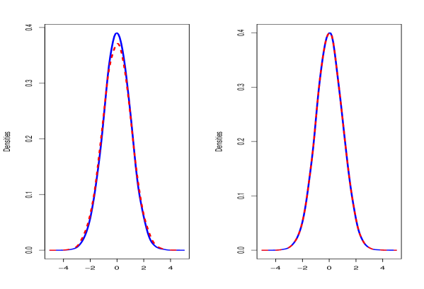
Figure 1: Curves of the densities $\widetilde{f}_{n}$ (dashed line) and $\widehat{f}_{n}$ (solid line) in univariate case for $c_{0}=1$ and for sample sizes $n=50$ (left side) and $n=100$ (right side). All the values of $\widetilde{f}_{n}$ and $\widehat{f}_{n}$ are calculated from $300$ replicates of generated data.

$e$	$n$	$c_{0}$	Estimator $\widetilde{f}_{n}$			Estimator $\widehat{f}_{n}$
			Bias	Variance	MSE	Bias	Variance	MSE
$-1$	50	$0.25$	0.2380	0.0080	0.0647	0.1592	0.0062	0.0316
		0.5	0.2380	0.0080	0.0647	0.2185	0.0069	0.0547
		1	0.2380	0.0080	0.0647	0.2357	0.0071	0.0627
	100	$0.25$	-0.0019	0.0034	0.0034	-0.0038	0.0027	0.0027
		0.5	-0.0019	0.0034	0.0034	-0.0026	0.0034	0.0034
		1	-0.0019	0.0034	0.0034	0.0022	0.0030	0.0030
$0$	50	$0.25$	0.3843	0.0106	0.1583	0.1291	0.0111	0.0278
		0.5	0.3843	0.0106	0.1583	0.2391	0.0079	0.0646
		1	0.3843	0.0106	0.1583	0.2886	0.0104	0.0937
	100	$0.25$	0.0008	0.0054	0.0054	-0.0440	0.0044	0.0063
		0.5	0.0008	0.0054	0.0054	-0.0242	0.0053	0.0059
		1	0.0008	0.0054	0.0054	-0.0137	0.0050	0.0062
$1$	50	$0.25$	0.2391	0.0079	0.0651	0.1557	0.0579	0.0300
		0.5	0.2391	0.0079	0.0651	0.2122	0.0069	0.0520
		1	0.2391	0.0079	0.0651	0.2275	0.0071	0.0589
	100	$0.25$	-0.0007	0.0038	0.0038	-0.0042	0.0033	0.0033
		0.5	-0.0007	0.0038	0.0038	-0.0058	0.0034	0.0035
		1	-0.0007	0.0038	0.0038	-0.0063	0.0033	0.0034

Table 1: The table compares some values of the bias, variance and mean square error of the estimators $\widetilde{f}_{n}$ and $\widehat{f}_{n}$ when the data are generated from Model 5.1. All these values are based on $300$ simulations runs.

5.2 Trivariate case

We consider the model

$$Y=1+X_{1}+X_{2}^{2}+\sin(\pi X_{3})+\varepsilon,$$ (5.2)

where $\varepsilon\sim N(0,1)$ and $X_{1},X_{2},X_{3}\sim U[0,1]$. As in the univariate case, our study is based on $300$ simulation runs. We use the kernels $K_{1}(x)=(15/16)(1-x^{2})^{2}\mathds{1}(|x|\leq 1)$, $K_{0}(x_{1},x_{2},x_{3})=\prod_{j=1}^{3}K_{1}(x_{j})$ and consider $\mathcal{X}_{0}=[\delta,1-\delta]^{3}$, $\delta=0.001$. We use the bandwidths

$$b_{1}=\widetilde{b}_{1},\quad b_{0}=c_{0}\times\max\left\{\left(\frac{1}{n^{2}b_{1}^{3}}\right)^{\frac{1}{d+4}},\left(\frac{1}{n^{3}b_{1}^{7}}\right)^{\frac{1}{2d+4}}\right\}=c_{0}\left(\frac{1}{n^{2}b_{1}^{3}}\right)^{\frac{1}{7}},$$

where $d=3$, $c_{0}\in[0,1]$ and $\widetilde{b}_{1}$ is the average standard deviation on the generated errors.

FIGURE 2 HERE

Figure 2 compares the curves of $\widetilde{f}_{n}(e)$ and $\widehat{f}_{n}(e)$ for $c_{0}=1$ and sample sizes $n=100$ and $n=200$. We note a difference between the curves at the neighborhood of the inflexion point $e=0$. But this difference is less important for $n=200$. This augurs that for $e$ very close to $0$, the difference between $\widehat{f}_{n}(e)$ and $\widetilde{f}_{n}(e)$ should be negligible only when the size of the samples is large enough.

TABLE 2 HERE

In Table 2 we give some values of the bias, variance and mean square error of $\widetilde{f}_{n}(e)$ and $\widehat{f}_{n}(e)$ for $c_{0}=0.25$, $0.5$ and $1$. We see that the mean square error of $\widehat{f}_{n}(e)$ is greater than the one of $\widetilde{f}_{n}(e)$. Further, we observe that the performance of $\widehat{f}_{n}(e)$ should be sensitive to the choice of the constant $c_{0}$. For example, for $e=0$, $c_{0}=0.5$ and $c_{0}=1$, the mean square error of $\widehat{f}_{n}(e)$ is very high compared to the sum of the variance and the square of the bias.

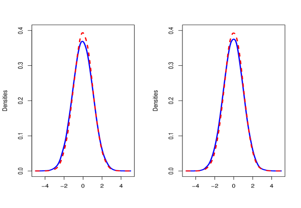
Figure 2: Curves of the densities $\widetilde{f}_{n}$ (dashed line) and $\widehat{f}_{n}$ (solid line) in trivariate case for $c_{0}=1$ and for sample sizes $n=100$ (left side) and $n=200$ (right side). The values are computed from $300$ simulation runs.

$e$	$n$	$c_{0}$	Estimator $\widetilde{f}_{n}$			Estimator $\widehat{f}_{n}$
			Bias	Variance	MSE	Bias	Variance	MSE
$-1$	100	$0.25$	-0.0013	0.0035	0.0036	-0.1250	0.0015	0.0539
		0.5	-0.0013	0.0035	0.0036	-0.0180	0.0027	0.0416
		1	-0.0013	0.0035	0.0036	0.0064	0.0027	0.0483
	200	$0.25$	0.0020	0.0019	0.0019	-0.1078	0.0011	0.0531
		0.5	0.0020	0.0019	0.0019	-0.0114	0.0014	0.0431
		1	0.0020	0.0019	0.0019	0.0017	0.0015	0.0525
$0$	100	$0.25$	-0.0049	0.0047	0.0047	-0.1858	0.0042	0.0329
		0.5	-0.0049	0.0047	0.0047	-0.0930	0.0045	0.1451
		1	-0.0049	0.0047	0.0047	-0.0377	0.0044	0.3318
	200	$0.25$	-0.0024	0.0030	0.0030	-0.1713	0.0028	0.0378
		0.5	-0.0024	0.0030	0.0030	-0.0764	0.0030	0.1817
		1	-0.0024	0.0030	0.0030	-0.0297	0.0026	0.3591
$1$	100	$0.25$	-0.0020	0.0031	0.0031	0.0341	0.0031	0.0419
		0.5	-0.0020	0.0031	0.0031	-0.0131	0.0025	0.0033
		1	-0.0020	0.0031	0.0031	-0.0010	0.0028	0.0416
	200	$0.25$	-0.0064	0.0019	0.0019	0.0239	0.0020	0.0325
		0.5	-0.0006	0.0019	0.0019	-0.0101	0.0016	0.0062
		1	-0.0006	0.0019	0.0019	-0.0126	0.0016	0.0477

Table 2: The table gives some values of the bias, variance and mean square error of $\widetilde{f}_{n}$ and $\widehat{f}_{n}$ when data are generated from Model 5.2. All values are based on $300$ replications of simulated data.

6 Conclusion

The aim of this paper was to investigate the nonparametric kernel estimation of the probability density function of the regression error using the estimated residuals. First, we evaluated the impact of the estimation of the regression function on the error density estimator. To this aim, the difference between the feasible density estimator based on the estimated residuals and the unfeasible one using the true errors was investigated. Second, the optimal choices of the first and second step bandwidths used for estimating the regression function and the error density were proposed. Further, we establish the asymptotic normality of the feasible estimator. The strategy used here to estimate the error density is based on a two-steps procedure which, in a first step, replaces the unobserved residuals terms by some nonparametric estimators $\widehat{\varepsilon}_{i}=Y_{i}-\widehat{m}_{n}(X_{i})$, where $\widehat{m}_{n}(X_{i})$ is a nonparametric estimator of $m(X_{i})$. In a second step, the estimated residuals $\widehat{\varepsilon}_{i}$ are used to estimate the error density $f(\cdot)$, as if they were the true $\varepsilon_{i}$’s. Though proceeding may remedy the curse of dimensionality for large sample sizes, a challenging issue was to evaluate the impact of the estimated residuals on the estimation of $f(\cdot)$, and to find the order of the optimal first-step bandwidth $b_{0}$ used for estimating the error terms. For the choice of $b_{0}$, our results show that the ideal bandwidth for $b_{0}$ should be smaller than the optimal bandwidth for the nonparametric kernel estimation of $m(\cdot)$. This means that the best estimator of $m(\cdot)$ needed for estimating $f(\cdot)$ should have a lower bias and a higher variance than the classical kernel regression estimator. With this ideal choice of $b_{0}$, we establish that for $d\leq 2$, the estimator $\widehat{f}_{n}(e)$ of $f(e)$ can attain the convergence rate $n^{-2/5}$, which corresponds to the optimal consistency rate achieved by the univariate kernel density estimator. For $d\geq 3$, the rate $n^{-2/5}$ is not reachable by our estimator $\widehat{f}_{n}(e)$. However, the rate we obtain for $\widehat{f}_{n}(e)$ is better than the optimal one achieved in the case of the kernel estimation of a multivariate density.

7 Proofs section

Intermediate Lemmas for Theorem 4.1

Lemma 7.1.

Define, for $x\in\mathcal{X}_{0}$,

$$\widehat{g}_{n}(x)=\frac{1}{nb_{0}^{d}}\sum_{i=1}^{n}K_{0}\left(\frac{X_{i}-x}{b_{0}}\right),\quad\overline{g}_{n}(x)=\mathbb{E}\left[\widehat{g}_{n}(x)\right].$$

Then under ${\rm(A_{1})-(A_{2})}$, ${\rm(A_{6})}$ and ${\rm(A_{8})}$, we have, when $b_{0}$ goes to $0$,

$$\sup_{x\in\mathcal{X}_{0}}\left|\overline{g}_{n}(x)-g(x)\right|=O\left(b_{0}^{2}\right),\quad\sup_{x\in\mathcal{X}_{0}}\left|\widehat{g}_{n}(x)-\overline{g}_{n}(x)\right|=O_{\mathbb{P}}\left(b_{0}^{4}+\frac{\ln n}{nb_{0}^{d}}\right)^{1/2},$$

and

$$\sup_{x\in\mathcal{X}_{0}}\left|\frac{1}{\widehat{g}_{n}(x)}-\frac{1}{g(x)}\right|=O_{\mathbb{P}}\left(b_{0}^{4}+\frac{\ln n}{nb_{0}^{d}}\right)^{1/2}.$$

Lemma 7.2.

Set

$$f_{in}(e)=\frac{\mathds{1}\left(X_{i}\in\mathcal{X}_{0}\right)}{b_{1}\mathbb{P}\left(X\in\mathcal{X}_{0}\right)}K_{1}\left(\frac{\varepsilon_{i}-e}{b_{1}}\right).$$

Then under ${\rm(A_{4})}$, ${\rm(A_{5})}$ and ${\rm(A_{7})}$, we have, for $b_{1}$ going to $0$, and for some constant $C>0$,

$$\mathbb{E}f_{in}(e) = f(e)+\frac{b_{1}^{2}}{2}f^{(2)}(e)\int v^{2}K_{1}(v)dv+o\left(b_{1}^{2}\right),$$

$$\hbox{\rm Var}\left(f_{in}(e)\right) = \frac{f(e)}{b_{1}\mathbb{P}\left(X\in\mathcal{X}_{0}\right)}\int K_{1}^{2}(v)dv+o\left(\frac{1}{b_{1}}\right),$$

$$\mathbb{E}\left|f_{in}(e)-\mathbb{E}f_{in}(e)\right|^{3} \leq \frac{Cf(e)}{b_{1}^{2}\mathbb{P}^{2}\left(X\in\mathcal{X}_{0}\right)}\int\left|K_{1}(v)\right|^{3}dv+o\left(\frac{1}{b_{1}^{2}}\right).$$

Lemma 7.3.

Define

$$S_{n} = \sum_{i=1}^{n}\mathds{1}\left(X_{i}\in\mathcal{X}_{0}\right)\left(\widehat{m}_{in}-m(X_{i})\right)K_{1}^{(1)}\left(\frac{\varepsilon_{i}-e}{b_{1}}\right),$$

$$T_{n} = \sum_{i=1}^{n}\mathds{1}\left(X_{i}\in\mathcal{X}_{0}\right)\left(\widehat{m}_{in}-m(X_{i})\right)^{2}K_{1}^{(2)}\left(\frac{\varepsilon_{i}-e}{b_{1}}\right),$$

$$R_{n} = \sum_{i=1}^{n}\mathds{1}\left(X_{i}\in\mathcal{X}_{0}\right)\left(\widehat{m}_{in}-m(X_{i})\right)^{3}\int_{0}^{1}(1-t)^{2}K_{1}^{(3)}\left(\frac{\varepsilon_{i}-t(\widehat{m}_{in}-m(X_{i}))-e}{b_{1}}\right)dt.$$

Then under ${\rm(A_{1})-(A_{9})}$, we have, for $b_{0}$ and $b_{1}$ small enough,

$$S_{n} = O_{\mathbb{P}}\left[b_{0}^{2}\left(nb_{1}^{2}+(nb_{1})^{1/2}\right)+\left(nb_{1}^{4}+\frac{b_{1}}{b_{0}^{d}}\right)^{1/2}\right],$$

$$T_{n} = O_{\mathbb{P}}\left[\left(nb_{1}^{3}+\left(nb_{1}\right)^{1/2}+\left(n^{2}b_{0}^{d}b_{1}^{3}\right)^{1/2}\right)\left(b_{0}^{4}+\frac{1}{nb_{0}^{d}}\right)\right],$$

$$R_{n} = O_{\mathbb{P}}\left[\left(nb_{1}^{3}+\left(n^{2}b_{0}^{d}b_{1}\right)^{1/2}\right)\left(b_{0}^{4}+\frac{1}{nb_{0}^{d}}\right)^{3/2}\right].$$

Lemma 7.4.

Under ${\rm(A_{5})}$ and ${\rm(A_{7})}$ we have, for some constant $C>0$, and for any $e$ in $\mathbb{R}$ and $p\in[0,2]$,

$$\left|\int K_{1}^{(1)}\left(\frac{e-e}{b_{1}}\right)^{2}e^{p}f(e)de\right|\leq Cb_{1}, \left|\int K_{1}^{(1)}\left(\frac{e-e}{b_{1}}\right)e^{p}f(e)de\right|\leq Cb_{1}^{2},$$ (7.1)

$$\left|\int K_{1}^{(2)}\left(\frac{e-e}{b_{1}}\right)^{2}e^{p}f(e)de\right|\leq Cb_{1}, \left|\int K_{1}^{(2)}\left(\frac{e-e}{b_{1}}\right)e^{p}f(e)de\right|\leq Cb_{1}^{3},$$ (7.2)

$$\left|\int K_{1}^{(3)}\left(\frac{e-e}{b_{1}}\right)^{2}e^{p}f(e)de\right|\leq Cb_{1}, \left|\int K_{1}^{(3)}\left(\frac{e-e}{b_{1}}\right)e^{p}f(e)de\right|\leq Cb_{1}^{3}.$$ (7.3)

Lemma 7.5.

Let

$$\beta_{in}=\frac{\mathds{1}\left(X_{i}\in\mathcal{X}_{0}\right)}{nb_{0}^{d}\widehat{g}_{in}}\sum_{j=1,j\neq i}^{n}\left(m(X_{j})-m(X_{i})\right)K_{0}\left(\frac{X_{j}-X_{i}}{b_{0}}\right),$$

where

$$\widehat{g}_{in}=\frac{1}{nb_{0}^{d}}\sum_{j=1\atop j\neq i}^{n}K_{0}\left(\frac{X_{j}-X_{i}}{b_{0}}\right).$$

Then, under ${\rm(A_{1})-(A_{9})}$, we have, when $b_{0}$ and $b_{1}$ go to $0$,

$$\sum_{i=1}^{n}\beta_{in}K_{1}^{(1)}\left(\frac{\varepsilon_{i}-e}{b_{1}}\right)=O_{\mathbb{P}}\left(b_{0}^{2}\right)\left(nb_{1}^{2}+(nb_{1})^{1/2}\right).$$

Lemma 7.6.

Let

$$\Sigma_{in}=\frac{\mathds{1}\left(X_{i}\in\mathcal{X}_{0}\right)}{nb_{0}^{d}\widehat{g}_{in}}\sum_{j=1,j\neq i}^{n}\varepsilon_{j}K_{0}\left(\frac{X_{j}-X_{i}}{b_{0}}\right).$$

Then, under ${\rm(A_{1})-(A_{9})}$, we have

$$\sum_{i=1}^{n}\Sigma_{in}K_{1}^{(1)}\left(\frac{\varepsilon_{i}-e}{b_{1}}\right)=O_{\mathbb{P}}\left(nb_{1}^{4}+\frac{b_{1}}{b_{0}^{d}}\right)^{1/2}.$$

Lemma 7.7.

Let $\mathbb{E}_{n}[\cdot]$ be the conditional mean given $X_{1},\ldots,X_{n}$. Then under ${\rm(A_{1})-(A_{9})}$, we have

$$\sup_{1\leq i\leq n}\mathbb{E}_{n}\biggl{[}\mathds{1}\left(X_{i}\in\mathcal{X}_{0}\right)(\widehat{m}_{in}-m(X_{i}))^{4}\biggr{]} = O_{\mathbb{P}}\left(b_{0}^{4}+\frac{1}{nb_{0}^{d}}\right)^{2},$$

$$\sup_{1\leq i\leq n}\mathbb{E}_{n}\biggl{[}\mathds{1}\left(X_{i}\in\mathcal{X}_{0}\right)(\widehat{m}_{in}-m(X_{i}))^{6}\biggr{]} = O_{\mathbb{P}}\left(b_{0}^{4}+\frac{1}{nb_{0}^{d}}\right)^{3}.$$

Lemma 7.8.

Assume that $(A_{4})$ and $(A_{6})$ hold. Then, for any $1\leq i\neq j\leq n$, and for any $e$ in $\mathbb{R}$,

$$\left(\widehat{m}_{in}-m(X_{i}),\varepsilon_{i}\right)\mbox{\it and }\left(\widehat{m}_{jn}-m(X_{j}),\varepsilon_{j}\right)$$

are independent given $X_{1},\ldots,X_{n}$, provided that $\|X_{i}-X_{j}\|\geq Cb_{0}$, for some constant $C>0$.

Lemma 7.9.

Let $\hbox{\rm Var}_{n}(\cdot)$ and $Cov_{n}(\cdot)$ be respectively the conditional variance and the conditional covariance given $X_{1},\ldots,X_{n}$, and set

$$\zeta_{in}=\mathds{1}\left(X_{i}\in\mathcal{X}_{0}\right)(\widehat{m}_{in}-m(X_{i}))^{2}K_{1}^{(2)}\left(\frac{\varepsilon_{i}-e}{b_{1}}\right).$$

Then under $(A_{1})-(A_{9})$, we have, for $n$ going to infinity,

$$\sum_{i=1}^{n}\hbox{\rm Var}_{n}\left(\zeta_{in}\right) = O_{\mathbb{P}}\left(nb_{1}\right)\left(b_{0}^{4}+\frac{1}{nb_{0}^{d}}\right)^{2},$$

$$\sum_{i=1}^{n}\sum_{j=1\atop j\neq i}^{n}\hbox{\rm Cov}_{n}\left(\zeta_{in},\zeta_{jn}\right) = O_{\mathbb{P}}\left(n^{2}b_{0}^{d}b_{1}^{7/2}\right)\left(b_{0}^{4}+\frac{1}{nb_{0}^{d}}\right)^{2}.$$

All these lemmas are proved in Appendix A.

Proof of Theorem 4.1

The proof of the theorem is based on the following equalities:

$$\widehat{f}_{n}(e)-\widetilde{f}_{n}(e) = O_{\mathbb{P}}\left[b_{0}^{2}+\left(\frac{1}{n}+\frac{1}{n^{2}b_{0}^{d}b_{1}^{3}}\right)^{1/2}\right]+O_{\mathbb{P}}\left[\frac{1}{(nb_{1}^{5})^{1/2}}+\left(\frac{b_{0}^{d}}{b_{1}^{3}}\right)^{1/2}\right]\left(b_{0}^{4}+\frac{1}{nb_{0}^{d}}\right)$$ (7.4)

$$+\;O_{\mathbb{P}}\left[\frac{1}{b_{1}}+\left(\frac{b_{0}^{d}}{b_{1}^{7}}\right)^{1/2}\right]\left(b_{0}^{4}+\frac{1}{nb_{0}^{d}}\right)^{3/2},$$

and

$$\widetilde{f}_{n}(e)-f(e)=O_{\mathbb{P}}\left(b_{1}^{4}+\frac{1}{nb_{1}}\right)^{1/2}.$$ (7.5)

Indeed, since $\widehat{f}_{n}(e)-f(e)=(\widetilde{f}_{n}(e)-f(e))+\widehat{f}_{n}(e)-\widetilde{f}_{n}(e)$, it then follows by (7.5) and (7.4) that

$$\widehat{f}_{n}(e)-f(e) = O_{\mathbb{P}}\left[b_{1}^{4}+\frac{1}{nb_{1}}+b_{0}^{4}+\frac{1}{n}+\frac{1}{n^{2}b_{0}^{d}b_{1}^{3}}+\left(\frac{1}{(nb_{1}^{5})^{1/2}}+\left(\frac{b_{0}^{d}}{b_{1}^{3}}\right)^{1/2}\right)^{2}\left(b_{0}^{4}+\frac{1}{nb_{0}^{d}}\right)^{2}\right]^{1/2}$$

$$+\;O_{\mathbb{P}}\left[\left(\frac{1}{b_{1}}+\left(\frac{b_{0}^{d}}{b_{1}^{7}}\right)^{1/2}\right)^{2}\left(b_{0}^{4}+\frac{1}{nb_{0}^{d}}\right)^{3}\right]^{1/2}.$$

This yields the result of the Theorem, since under ${\rm(A_{8})}$ and ${\rm(A_{9})}$, we have

$$\frac{1}{n}=O\left(\frac{1}{nb_{1}}\right),\quad\frac{1}{n^{2}b_{0}^{d}b_{1}^{3}}=O\left(\frac{b_{0}^{d}}{b_{1}^{3}}\right)\left(b_{0}^{4}+\frac{1}{nb_{0}^{d}}\right)^{2}.$$

Hence, it remains to prove equalities (7.4) and (7.5). For this, define $S_{n}$, $R_{n}$ and $T_{n}$ as in the statement of Lemma 7.3. Since $\widehat{\varepsilon}_{i}-\varepsilon_{i}=-\left(\widehat{m}_{in}-m(X_{i})\right)$ and that $K_{1}$ is three times continuously differentiable under ${\rm(A_{7})}$, the third-order Taylor expansion with integral remainder gives

$$\widehat{f}_{1n}(e)-\widetilde{f}_{n}(e) = \frac{1}{b_{1}\sum_{i=1}^{n}\mathds{1}(X_{i}\in\mathcal{X}_{0})}\sum_{i=1}^{n}\mathds{1}\left(X_{i}\in\mathcal{X}_{0}\right)\left[K_{1}\left(\frac{\widehat{\varepsilon}_{i}-e}{b_{1}}\right)-K_{1}\left(\frac{\varepsilon_{i}-e}{b_{1}}\right)\right]$$

$$= -\frac{1}{b_{1}\sum_{i=1}^{n}\mathds{1}(X_{i}\in\mathcal{X}_{0})}\left(\frac{S_{n}}{b_{1}}-\frac{T_{n}}{2b_{1}^{2}}+\frac{R_{n}}{2b_{1}^{3}}\right).$$

Therefore, since

$$\sum_{i=1}^{n}\mathds{1}\left(X_{i}\in\mathcal{X}_{0}\right)=n\left(\mathbb{P}\left(X\in\mathcal{X}_{0}\right)+o_{\mathbb{P}}(1)\right),$$

by the Law of large numbers, Lemma 7.3 then gives

$$\widehat{f}_{n}(e)-\widetilde{f}_{n}(e)=O_{\mathbb{P}}\left(\frac{1}{nb_{1}^{2}}\right)S_{n}+O_{\mathbb{P}}\left(\frac{1}{nb_{1}^{3}}\right)T_{n}+O_{\mathbb{P}}\left(\frac{1}{nb_{1}^{4}}\right)R_{n}$$

$$= O_{\mathbb{P}}\left[b_{0}^{2}\left(1+\frac{1}{(nb_{1}^{3})^{1/2}}\right)+\left(\frac{1}{n}+\frac{1}{n^{2}b_{0}^{d}b_{1}^{3}}\right)^{1/2}\right]$$

$$+\;O_{\mathbb{P}}\left[1+\frac{1}{(nb_{1}^{5})^{1/2}}+\left(\frac{b_{0}^{d}}{b_{1}^{3}}\right)^{1/2}\right]\left(b_{0}^{4}+\frac{1}{nb_{0}^{d}}\right)+O_{\mathbb{P}}\left[\frac{1}{b_{1}}+\left(\frac{b_{0}^{d}}{b_{1}^{7}}\right)^{1/2}\right]\left(b_{0}^{4}+\frac{1}{nb_{0}^{d}}\right)^{3/2}.$$

This yields (7.4), since under ${\rm(A_{8})}$ and ${\rm(A_{9})}$, we have $b_{0}\rightarrow 0$, $nb_{0}^{d+2}\rightarrow\infty$ and $nb_{1}^{3}\rightarrow\infty$, so that

$$b_{0}^{2}\left(1+\frac{1}{(nb_{1}^{3})^{1/2}}\right) \asymp O\left(b_{0}^{2}\right),\quad\left(b_{0}^{4}+\frac{1}{nb_{0}^{d}}\right)=O\left(b_{0}^{2}\right),$$

$$\left[1+\frac{1}{(nb_{1}^{5})^{1/2}}+\left(\frac{b_{0}^{d}}{b_{1}^{3}}\right)^{1/2}\right]\left(b_{0}^{4}+\frac{1}{nb_{0}^{d}}\right) = O\left(b_{0}^{2}\right)+\left[\frac{1}{(nb_{1}^{5})^{1/2}}+\left(\frac{b_{0}^{d}}{b_{1}^{3}}\right)^{1/2}\right]\left(b_{0}^{4}+\frac{1}{nb_{0}^{d}}\right).$$

For (7.5), note that

$$\mathbb{E}_{n}\left[\left(\widetilde{f}_{n}(e)-f(e)\right)^{2}\right]=\hbox{\rm Var}_{n}\left(\widetilde{f}_{n}(e)\right)+\biggl{(}\mathbb{E}_{n}\left[\widetilde{f}_{n}(e)\right]-f(e)\biggr{)}^{2},$$ (7.6)

with, using ${\rm(A_{4})}$,

$$\hbox{\rm Var}_{n}\left(\widetilde{f}_{n}(e)\right)=\frac{1}{\left(b_{1}\sum_{i=1}^{n}\mathds{1}\left(X_{i}\in\mathcal{X}_{0}\right)\right)^{2}}\sum_{i=1}^{n}\mathds{1}\left(X_{i}\in\mathcal{X}_{0}\right)\hbox{\rm Var}\left[K_{1}\left(\frac{\varepsilon-e}{b_{1}}\right)\right].$$

Therefore, since the Cauchy-Schwarz inequality gives

$$\hbox{\rm Var}\left[K_{1}\left(\frac{\varepsilon-e}{b_{1}}\right)\right]\leq\mathbb{E}\left[K_{1}^{2}\left(\frac{\varepsilon-e}{b_{1}}\right)\right]=b_{1}\int K_{1}^{2}(v)f(e+b_{1}v)dv,$$

this bound and the equality above yield, under ${\rm(A_{5})}$ and ${\rm(A_{7})}$,

$$\hbox{\rm Var}_{n}\left(\widetilde{f}_{n}(e)\right)\leq\frac{C}{b_{1}\sum_{i=1}^{n}\mathds{1}\left(X_{i}\in\mathcal{X}_{0}\right)}=O_{\mathbb{P}}\left(\frac{1}{nb_{1}}\right).$$ (7.7)

For the second term in (7.6), we have

$$\mathbb{E}_{n}\left[\widetilde{f}_{n}(e)\right]=\frac{1}{b_{1}\sum_{i=1}^{n}\mathds{1}\left(X_{i}\in\mathcal{X}_{0}\right)}\sum_{i=1}^{n}\mathds{1}\left(X_{i}\in\mathcal{X}_{0}\right)\mathbb{E}\left[K_{1}\left(\frac{\varepsilon-e}{b_{1}}\right)\right].$$ (7.8)

By ${\rm(A_{7})}$, $K_{1}$ is symmetric, has a compact support, with $\int\!vK_{1}(v)=0$ and $\int\!K_{1}(v)dv=1$. Therefore, since $f(\cdot)$ has bounded continuous second order derivatives under $(A_{5})$, this yields for some $\theta=\theta(e,b_{1}v)$,

$$\mathbb{E}\left[K_{1}\left(\frac{\varepsilon-e}{b_{1}}\right)\right]=b_{1}\int K_{1}(v)f(e+b_{1}v)dv$$ (7.9)

$$= b_{1}\int K_{1}(v)\left[f(e)+b_{1}vf^{(1)}(e)+\frac{b_{1}^{2}v^{2}}{2}f^{(2)}(e+\theta b_{1}v)\right]dv$$

$$= b_{1}f(e)+\frac{b_{1}^{3}}{2}\int v^{2}K_{1}(v)f^{(2)}(e+\theta b_{1}v)dv.$$

Hence this equality and (7.8) give

$$\mathbb{E}_{n}\left[\widetilde{f}_{n}(e)\right]=f(e)+\frac{b_{1}^{2}}{2}\int v^{2}K_{1}(v)f^{(2)}(e+\theta b_{1}v)dv,$$

so that

$$\biggl{(}\mathbb{E}_{n}\left[\widetilde{f}_{n}(e)\right]-f(e)\biggr{)}^{2}=O_{\mathbb{P}}\left(b_{1}^{4}\right).$$

Combining this result with (7.7) and (7.6), we obtain, by the Tchebychev inequality,

$$\widetilde{f}_{n}(e)-f(e)=O_{\mathbb{P}}\left(b_{1}^{4}+\frac{1}{nb_{1}}\right)^{1/2}.$$

This proves (7.5) and achieves the proof of the theorem. $\Box$

Proof of Theorem 4.2

Recall that

$$R_{n}(b_{0},b_{1})=b_{0}^{4}+\left[\frac{1}{(nb_{1}^{5})^{1/2}}+\left(\frac{b_{0}^{d}}{b_{1}^{3}}\right)^{1/2}\right]^{2}\left(b_{0}^{4}+\frac{1}{nb_{0}^{d}}\right)^{2}+\left[\frac{1}{b_{1}}+\left(\frac{b_{0}^{d}}{b_{1}^{7}}\right)^{1/2}\right]^{2}\left(b_{0}^{4}+\frac{1}{nb_{0}^{d}}\right)^{3},$$

and note that

$$\left(\frac{1}{n^{2}b_{1}^{3}}\right)^{\frac{1}{d+4}}=\max\left\{\left(\frac{1}{n^{2}b_{1}^{3}}\right)^{\frac{1}{d+4}},\left(\frac{1}{n^{3}b_{1}^{7}}\right)^{\frac{1}{2d+4}}\right\}$$

if and only if $n^{4-d}b_{1}^{d+16}\rightarrow\infty$. To find the order of $b_{0}^{*}$, we shall deal with the cases $nb_{0}^{d+4}\rightarrow\infty$ and $nb_{0}^{d+4}=O(1)$. First assume that $nb_{0}^{d+4}\rightarrow\infty$. More precisely, we suppose that $b_{0}$ is in $\left[(u_{n}/n)^{1/(d+4)},+\infty\right)$, where $u_{n}\rightarrow\infty$. Since $1/(nb_{0}^{d})=O(b_{0}^{4})$ for all these $b_{0}$, we have

$$\left(b_{0}^{4}+\frac{1}{nb_{0}^{d}}\right)^{2}\asymp\left(b_{0}^{4}\right)^{2},\quad\left(b_{0}^{4}+\frac{1}{nb_{0}^{d}}\right)^{3}\asymp\left(b_{0}^{4}\right)^{3}.$$

Hence the order of $b_{0}^{*}$ is computed by minimizing the function

$$b_{0}\rightarrow b_{0}^{4}+\left[\frac{1}{(nb_{1}^{5})^{1/2}}+\left(\frac{b_{0}^{d}}{b_{1}^{3}}\right)^{1/2}\right]^{2}\left(b_{0}^{4}\right)^{2}+\left[\frac{1}{b_{1}}+\left(\frac{b_{0}^{d}}{b_{1}^{7}}\right)^{1/2}\right]^{2}\left(b_{0}^{4}\right)^{3}.$$

Since this function is increasing with $b_{0}$, the minimum of $R_{n}(\cdot,b_{1})$ is achieved for $b_{0}^{**}=(u_{n}/n)^{1/(d+4)}$. We shall prove later on that this choice of $b_{0}^{**}$ is irrelevant compared to the one arising when $nb_{0}^{d+4}=O(1)$.

Consider now the case $nb_{0}^{d+4}=O(1)$ i.e $b_{0}^{4}=O\left(1/(nb_{0}^{d})\right)$. This gives

$$\left[\frac{1}{(nb_{1}^{5})^{1/2}}+\left(\frac{b_{0}^{d}}{b_{1}^{3}}\right)^{1/2}\right]^{2}\left(b_{0}^{4}+\frac{1}{nb_{0}^{d}}\right)^{2} \asymp \left(\frac{1}{nb_{1}^{5}}+\frac{b_{0}^{d}}{b_{1}^{3}}\right)\left(\frac{1}{n^{2}b_{0}^{2d}}\right),$$

$$\left[\frac{1}{b_{1}}+\left(\frac{b_{0}^{d}}{b_{1}^{7}}\right)^{1/2}\right]^{2}\left(b_{0}^{4}+\frac{1}{nb_{0}^{d}}\right)^{3} \asymp \left(\frac{1}{b_{1}^{2}}+\frac{b_{0}^{d}}{b_{1}^{7}}\right)\left(\frac{1}{n^{3}b_{0}^{3d}}\right).$$

Moreover if $nb_{0}^{d}b_{1}^{4}\rightarrow\infty$, we have, since $nb_{0}^{2d}\rightarrow\infty$ under ${\rm(A_{8})}$,

$$\left(\frac{1}{nb_{1}^{5}}+\frac{b_{0}^{d}}{b_{1}^{3}}\right)\left(\frac{1}{n^{2}b_{0}^{2d}}\right)\asymp\frac{b_{0}^{d}}{b_{1}^{3}}\left(\frac{1}{n^{2}b_{0}^{2d}}\right),\quad\left(\frac{1}{b_{1}^{2}}+\frac{b_{0}^{d}}{b_{1}^{7}}\right)\left(\frac{1}{n^{3}b_{0}^{3d}}\right)=O\left(\frac{b_{0}^{d}}{b_{1}^{3}}\right)\left(\frac{1}{n^{2}b_{0}^{2d}}\right).$$

Hence the order of $b_{0}^{*}$ is obtained by finding the minimum of the function $b_{0}^{4}+\left(1/n^{2}b_{0}^{d}b_{1}^{3}\right)$. The minimization of this function gives a solution $b_{0}$ such that

$$b_{0}\asymp\left(\frac{1}{n^{2}b_{1}^{3}}\right)^{\frac{1}{d+4}},\quad R_{n}(b_{0},b_{1})\asymp\left(\frac{1}{n^{2}b_{1}^{3}}\right)^{\frac{4}{d+4}}.$$

This value satisfies the constraints $nb_{0}^{d+4}=O(1)$ and $nb_{0}^{d}b_{1}^{4}\rightarrow\infty$ when $n^{4-d}b_{1}^{d+16}\rightarrow\infty$.

If now $nb_{0}^{d+4}=O(1)$ but $nb_{0}^{d}b_{1}^{4}=O(1)$, we have, since $nb_{0}^{2d}\rightarrow\infty$,

$$\frac{1}{nb_{1}^{5}}\left(\frac{1}{n^{2}b_{0}^{2d}}\right)=O\left(\frac{b_{0}^{d}}{b_{1}^{7}}\right)\left(\frac{1}{n^{3}b_{0}^{3d}}\right),\quad\frac{1}{b_{1}^{2}}\left(\frac{1}{n^{3}b_{0}^{3d}}\right)=O\left(\frac{b_{0}^{d}}{b_{1}^{3}}\right)\left(\frac{1}{n^{2}b_{0}^{2d}}\right)=O\left(\frac{b_{0}^{d}}{b_{1}^{7}}\right)\left(\frac{1}{n^{3}b_{0}^{3d}}\right).$$

In this case, $b_{0}^{*}$ is obtained by minimizing the function $b_{0}^{4}+\left(1/n^{3}b_{0}^{2d}b_{1}^{7}\right)$, for which the solution $b_{0}$ verifies

$$b_{0}\asymp\left(\frac{1}{n^{3}b_{1}^{7}}\right)^{\frac{1}{2d+4}},\quad R_{n}(b_{0},b_{1})\asymp\left(\frac{1}{n^{3}b_{1}^{7}}\right)^{\frac{4}{2d+4}}.$$

This solution fulfills the constraint $nb_{0}^{d}b_{1}^{4}=O(1)$ when $n^{4-d}b_{1}^{d+16}=O(1)$. Hence we can conclude that for $b_{0}^{4}=O\left(1/(nb_{0}^{d})\right)$, the bandwidth $b_{0}^{*}$ satisfies

$$b_{0}^{*}\asymp\max\left\{\left(\frac{1}{n^{2}b_{1}^{3}}\right)^{\frac{1}{d+4}},\left(\frac{1}{n^{3}b_{1}^{7}}\right)^{\frac{1}{2d+4}}\right\},$$

which leads to

$$R_{n}\left(b_{0}^{*},b_{1}\right)\asymp\max\left\{\left(\frac{1}{n^{2}b_{1}^{3}}\right)^{\frac{4}{d+4}},\left(\frac{1}{n^{3}b_{1}^{7}}\right)^{\frac{4}{2d+4}}\right\}.$$

We need now to compare the solution $b_{0}^{*}$ to the candidate $b_{0}^{**}=(u_{n}/n)^{1/(d+4)}$ obtained when $nb_{0}^{d+4}\rightarrow\infty$. For this, we must do a comparison between the orders of $R_{n}(b_{0}^{*},b_{1})$ and $R_{n}(b_{0}^{**},b_{1})$. Since $R_{n}(b_{0},b_{1})\geq b_{0}^{4}$ for all $b_{0}$, we have $R_{n}(b_{0}^{**},b_{1})\geq(u_{n}/n)^{4/(d+4)}$, so that

$$\frac{R_{n}(b_{0}^{*},b_{1})}{R_{n}(b_{0}^{**},b_{1})} \leq \left[\left(\frac{1}{n^{2}b_{1}^{3}}\right)^{\frac{1}{d+4}}+\left(\frac{1}{n^{3}b_{1}^{7}}\right)^{\frac{4}{2d+4}}\right]\left(\frac{n}{u_{n}}\right)^{\frac{4}{d+4}}$$

$$= o(1)+O\left(\frac{1}{u_{n}}\right)^{\frac{4}{d+4}}\left(\frac{1}{nb_{1}^{\frac{7(d+4)}{d+8}}}\right)^{\frac{4(d+8)}{(2d+4)(d+4)}}=o(1),$$

using the fact $n^{(d+8)}b_{1}^{7(d+4)}\rightarrow\infty$ by ${\rm(A_{9})}$ and that $u_{n}\rightarrow\infty$. This shows that $R_{n}(b_{0}^{*},b_{1})\leq R_{n}(b_{0}^{**},b_{1})$ for all $b_{1}$ and $n$ large enough. Hence the theorem is proved, since $b_{0}^{*}$ is the best candidate for the minimization of $R_{n}(\cdot,b_{1})$. $\Box$

Proof of Theorem 4.3

Recall that Theorem 4.2 gives

$$AMSE(b_{1})+R_{n}(b_{0}^{*},b_{1})\asymp r_{1}(b_{1})+r_{2}(b_{1})+r_{3}(b_{1})=F(b_{1}),$$

where

$$r_{1}(h) = h^{4}+\frac{1}{nh},\quad\arg\min r_{1}(h)\asymp n^{-1/5}=h_{1}^{*},\quad\min r_{1}(h)\asymp(h_{1}^{*})^{4}=n^{-4/5},$$

$$r_{2}(h) = h^{4}+\frac{1}{n^{\frac{8}{d+4}}h^{\frac{12}{d+4}}},\quad\arg\min r_{2}(h)\asymp n^{-\frac{2}{d+7}}=h_{2}^{*},\quad\min r_{2}(h)\asymp(h_{2}^{*})^{4}=n^{-\frac{8}{d+7}},$$

$$r_{3}(h) = h^{4}+\frac{1}{n^{\frac{12}{2d+4}}h^{\frac{28}{2d+4}}},\quad\arg\min r_{3}(h)\asymp n^{-\frac{3}{2d+11}}=h_{3}^{*},\quad\min r_{3}(h)\asymp(h_{3}^{*})^{4}=n^{-\frac{12}{2d+11}}.$$

Each $r_{j}(h)$ decreases on $\left[0,\arg\min r_{j}(h)\right]$ and increases on $\left(\arg\min r_{j}(h),\infty\right)$ and that $r_{j}(h)\asymp h^{4}$ on $\left(\arg\min r_{j}(h),\infty\right)$. Moreover $\min r_{2}(h)=o\left(r_{3}(h)\right)$ and $h_{2}^{*}=o\left(h_{3}^{*}\right)$ for all possible dimension $d$, so that $\min\{r_{2}(h)+r_{3}(h)\}\asymp(h_{3}^{*})^{4}=n^{-\frac{12}{2d+11}}$ and $\arg\min\{r_{2}(h)+r_{3}(h)\}\asymp h_{3}^{*}=n^{-\frac{3}{2d+11}}$.

Observe now that $\min\{r_{2}(h)+r_{3}(h)\}=O\left(\min r_{1}(h)\right)$ is equivalent to $n^{-\frac{12}{2d+11}}=O\left(n^{-4/5}\right)$ which holds if and only if $d\leq 2$. Hence assume that $d\leq 2$. Since $n^{-\frac{12}{2d+11}}=O\left(n^{-4/5}\right)$ also gives $\arg\min\{r_{2}(h)+r_{3}(h)\}\asymp h_{3}^{*}=O\left(h_{1}^{*}\right)$, we have

$$\min F(b_{1})\asymp n^{-4/5}\;\;{\rm and}\;\arg\min F(b_{1})\asymp n^{-1/5}.$$

The case $d>2$ is symmetric with

$$\min F(b_{1})\asymp n^{-\frac{12}{2d+11}}\;\;{\rm and}\;\arg\min F(b_{1})\asymp n^{-\frac{3}{2d+11}}.$$

This ends the proof of the theorem. $\Box$

Proof of Theorem 4.4

Observe that the Tchebychev inequality gives

$$\sum_{i=1}^{n}\mathds{1}\left(X_{i}\in\mathcal{X}_{0}\right)=n\mathbb{P}\left(X\in\mathcal{X}_{0}\right)\left[1+O_{\mathbb{P}}\left(\frac{1}{\sqrt{n}}\right)\right],$$

so that

$$\widetilde{f}_{n}(e)=\left[1+O_{\mathbb{P}}\left(\frac{1}{\sqrt{n}}\right)\right]f_{n}(e),$$

where

$$f_{n}(e)=\frac{1}{nb_{1}\mathbb{P}\left(X\in\mathcal{X}_{0}\right)}\sum_{i=1}^{n}\mathds{1}\left(X_{i}\in\mathcal{X}_{0}\right)K_{1}\left(\frac{\varepsilon_{i}-e}{b_{1}}\right).$$

Therefore

$$\widehat{f}_{n}(e)-\mathbb{E}f_{n}(e)=\left(f_{n}(e)-\mathbb{E}f_{n}(e)\right)+\left(\widehat{f}_{n}(e)-\widetilde{f}_{n}(e)\right)+O_{\mathbb{P}}\left(\frac{1}{\sqrt{n}}\right)f_{n}(e).$$ (7.10)

Let now $f_{in}(e)$ be as in the statement of Lemma 7.2, and note that $f_{n}(e)=(1/n)\sum_{i=1}^{n}f_{in}(e)$. The second and the third claims of Lemma 7.2 yield, since $nb_{1}$ diverges under ${\rm(A_{9})}$,

$$\frac{\sum_{i=1}^{n}\mathbb{E}\left|f_{in}(e)-\mathbb{E}f_{in}(e)\right|^{3}}{\left(\sum_{i=1}^{n}\hbox{\rm Var}f_{in}(e)\right)^{3/2}}\leq\frac{\frac{Cnf(e)}{\mathbb{P}\left(X\in\mathcal{X}_{0}\right)^{2}b_{1}^{2}}\displaystyle{\int}\left|K_{1}(v)\right|^{3}dv+o\left(\frac{n}{b_{1}^{2}}\right)}{\left(\frac{nf(e)}{\mathbb{P}\left(X\in\mathcal{X}_{0}\right)b_{1}}\displaystyle{\int}K_{1}^{2}(v)dv+o\left(\frac{n}{b_{1}}\right)\right)^{3/2}}=O(nb_{1})^{-1/2}=o(1).$$

Hence the Lyapounov Central Limit Theorem for triangular arrays (see e.g Billingsley 1968, Theorem 7.3) gives, since $nb_{1}$ diverges under ${\rm(A_{9})}$,

$$\frac{f_{n}(e)-\mathbb{E}f_{n}(e)}{\sqrt{\hbox{\rm Var}f_{n}(e)}}=\frac{f_{n}(e)-\mathbb{E}f_{n}(e)}{\sqrt{\frac{\hbox{\rm Var}f_{in}(e)}{n}}}\stackrel{{\scriptstyle d}}{{\rightarrow}}N\left(0,1\right).$$

This yields, using the second result of Lemma 7.2,

$$\sqrt{nb_{1}}\left(f_{n}(e)-\mathbb{E}f_{n}(e)\right)\stackrel{{\scriptstyle d}}{{\rightarrow}}N\left(0,\frac{f(e)}{\mathbb{P}\left(X\in\mathcal{X}_{0}\right)}\int K_{1}^{2}(v)dv\right).$$ (7.11)

Moreover, note that for $nb_{0}^{d}b_{1}^{3}\rightarrow\infty$ and $nb_{0}^{2d}\rightarrow\infty$, we have

$$\frac{1}{nb_{1}^{5}}\left(\frac{1}{nb_{0}^{d}}\right)^{2}+\left(\frac{1}{b_{1}^{2}}+\frac{b_{0}^{d}}{b_{1}^{7}}\right)\left(\frac{1}{nb_{0}^{d}}\right)^{3}=O\left(\frac{1}{n^{2}b_{0}^{d}b_{1}^{3}}+\frac{1}{n^{3}b_{0}^{2d}b_{1}^{7}}\right).$$

Therefore, since $b_{0}^{4}=O\left(1/(nb_{0}^{d})\right)$, $nb_{0}^{d}b_{1}^{3}\rightarrow\infty$ and $nb_{0}^{2d}\rightarrow\infty$ by $(\rm{A}_{10})$ and ${\rm(A_{8})}$, the equality above and (7.4) ensure that

$$\widehat{f}_{n}(e)-\widetilde{f}_{n}(e) = O_{\mathbb{P}}\left[b_{0}^{4}+\frac{1}{n}+\frac{1}{n^{2}b_{0}^{d}b_{1}^{3}}+\left(\frac{1}{nb_{1}^{5}}+\frac{b_{0}^{d}}{b_{1}^{3}}\right)\left(\frac{1}{nb_{0}^{d}}\right)^{2}+\left(\frac{1}{b_{1}^{2}}+\frac{b_{0}^{d}}{b_{1}^{7}}\right)\left(\frac{1}{nb_{0}^{d}}\right)^{3}\right]^{1/2}$$

$$= O_{\mathbb{P}}\left(b_{0}^{4}+\frac{1}{n}+\frac{1}{n^{2}b_{0}^{d}b_{1}^{3}}+\frac{1}{n^{3}b_{0}^{2d}b_{1}^{7}}\right)^{1/2}.$$

Hence for $b_{1}$ going to $0$, we have

$$\sqrt{nb_{1}}\left(\widehat{f}_{n}(e)-\widetilde{f}_{n}(e)\right)=O_{\mathbb{P}}\left[nb_{1}\left(b_{0}^{4}+\frac{1}{n}+\frac{1}{n^{2}b_{0}^{d}b_{1}^{3}}+\frac{1}{n^{3}b_{0}^{2d}b_{1}^{7}}\right)\right]^{1/2}=o_{\mathbb{P}}(1),$$

since $nb_{0}^{4}b_{1}=o(1)$ and that $nb_{0}^{d}b_{1}^{3}\rightarrow\infty$ under $(\rm{A}_{10})$. Combining the above result with (7.11) and (7.10), we obtain

$$\sqrt{nb_{1}}\left(\widehat{f}_{n}(e)-\mathbb{E}f_{n}(e)\right)\stackrel{{\scriptstyle d}}{{\rightarrow}}N\left(0,\frac{f(e)}{\mathbb{P}\left(X\in\mathcal{X}_{0}\right)}\int K_{1}^{2}(v)dv\right).$$

This ends the proof the Theorem, since the first result of Lemma 7.2 gives

$$\mathbb{E}f_{n}(e)=\mathbb{E}f_{1n}(e)=f(e)+\frac{b_{1}^{2}}{2}f^{(2)}(e)\int v^{2}K_{1}(v)dv+o\left(b_{1}^{2}\right):=\overline{f}_{n}(e).\Box$$

Appendix A: Proof of the intermediate results

Proof of Lemma 7.1

First note that by ${\rm(A_{6})}$, we have $\int\!zK_{0}(z)dz=0$ and $\int\!K_{0}(z)dz=1$. Therefore, since $K_{0}$ is continuous and has a compact support, ${\rm(A_{1})}$, ${\rm(A_{2})}$ and the second-order Taylor expansion yield, for $b_{0}$ small enough and any $x$ in $\mathcal{X}_{0}$,

$$\left|\overline{g}_{n}(x)-g(x)\right|=\left|\frac{1}{b_{0}^{d}}\int K_{0}\left(\frac{z-x}{b_{0}}\right)g(z)dz-g(x)\right|=\left|\int K_{0}(z)\left[g(x+b_{0}z)-g(x)\right]dz\right|$$

$$= \left|\int K_{0}(z)\left[b_{0}g^{(1)}(x)z+\frac{b_{0}^{2}}{2}zg^{(2)}(x+\theta b_{0}z)z^{\top}\right]dz\right|,\;\theta=\theta(x,b_{0}z)\in[0,1]$$

$$= \left|b_{0}g^{(1)}(x)\int zK_{0}(z)dz+\frac{b_{0}^{2}}{2}\int zg^{(2)}(x+\theta b_{0}z)z^{\top}K_{0}(z)dz\right|$$

$$= \frac{b_{0}^{2}}{2}\left|\int zg^{(2)}(x+\theta b_{0}z)z^{\top}K_{0}(z)dz\right|\leq Cb_{0}^{2}.$$

Therefore

$$\sup_{x\in\mathcal{X}_{0}}\left|\overline{g}_{n}(x)-g(x)\right|=O\left(b_{0}^{2}\right),$$

which gives the first result of the lemma. For the two last results of the lemma, it is sufficient to show that

$$\sup_{x\in\mathcal{X}_{0}}\left|\widehat{g}_{n}(x)-\overline{g}_{n}(x)\right|=O_{\mathbb{P}}\left(\frac{\ln n}{nb_{0}^{d}}\right)^{1/2},$$

since $\overline{g}_{n}(x)$ is asymptotically bounded away from $0$ over $\mathcal{X}_{0}$ and that $|\overline{g}_{n}(x)-g(x)|=O(b_{0}^{2})$ uniformly for $x$ in $\mathcal{X}_{0}$. This follows from Theorem 1 in Einmahl and Mason (2005). $\Box$

Proof of Lemma 7.2

For the first equality of the lemma, note that by ${\rm(A_{4})}$, ${\rm(A_{5})}$ and (7.9), we have

$$\mathbb{E}\left[f_{in}(e)\right]=\frac{1}{b_{1}}\mathbb{E}\left[K_{1}\left(\frac{\varepsilon-e}{b_{1}}\right)\right]=f(e)+\frac{b_{1}^{2}}{2}\int v^{2}K_{1}(v)f^{(2)}(e+\theta b_{1}v)dv.$$

Therefore the Lebesgue Dominated Convergence Theorem gives, for $b_{1}$ small enough,

$$\mathbb{E}\left[f_{in}(e)\right]-f(e)-\frac{b_{1}^{2}}{2}f^{(2)}(e)\int v^{2}K_{1}(v)dv$$

$$= \frac{b_{1}^{2}}{2}\int v^{2}K_{1}(v)\left[f^{(2)}\left(e+\theta b_{1}v\right)-f^{(2)}(e)\right]dv$$

$$= o\left(b_{1}^{2}\right).$$

This proves the first equality of the lemma. For the second and third results of the lemma, the proofs are straightforward. Hence they are omitted for the sake of brevity. $\Box$

Proof of Lemma 7.3

The order of $S_{n}$ follows from Lemmas 7.5 and 7.6. Indeed, since

$$\mathds{1}(X_{i}\in\mathcal{X}_{0})\left(\widehat{m}_{in}-m(X_{i})\right) = \frac{\mathds{1}(X_{i}\in\mathcal{X}_{0})}{nb_{0}^{d}\widehat{g}_{in}}\sum_{j=1,j\neq i}^{n}\left(m(X_{j})+\varepsilon_{j}-m(X_{i})\right)K_{0}\left(\frac{X_{j}-X_{i}}{b_{0}}\right)$$

$$= \beta_{in}+\Sigma_{in},$$

Lemmas 7.5 and 7.6 imply that

$$S_{n}=O_{\mathbb{P}}\left[b_{0}^{2}\left(nb_{1}^{2}+(nb_{1})^{1/2}\right)+\left(nb_{1}^{4}+\frac{b_{1}}{b_{0}^{d}}\right)^{1/2}\right],$$

which gives the desired result for $S_{n}$.

For the term $T_{n}$, the order is obtained by computing the conditional mean and the conditional variance given $X_{1},\ldots,X_{n}$. To this end, define for any $1\leq i\leq n$,

$$\mathbb{E}_{in}[\cdot]=\mathbb{E}_{n}\left[X_{1},\ldots,X_{n},\varepsilon_{k},k\neq i\right].$$

Therefore, since $(\widehat{m}_{in}-m(X_{i}))$ depends only upon $\left(X_{1},\ldots,X_{n},\varepsilon_{k},k\neq i\right)$, we have

$$\mathbb{E}_{n}[T_{n}] = \mathbb{E}_{n}\left[\sum_{i=1}^{n}\mathbb{E}_{in}\left[\mathds{1}\left(X_{i}\in\mathcal{X}_{0}\right)(\widehat{m}_{in}-m(X_{i}))^{2}K_{1}^{(2)}\left(\frac{\varepsilon_{i}-e}{b_{1}}\right)\right]\right]$$

$$= \mathbb{E}_{n}\left[\sum_{i=1}^{n}\mathds{1}\left(X_{i}\in\mathcal{X}_{0}\right)(\widehat{m}_{in}-m(X_{i}))^{2}\mathbb{E}_{in}\left[K_{1}^{(2)}\left(\frac{\varepsilon_{i}-e}{b_{1}}\right)\right]\right],$$

with, using ${\rm(A_{4})}$ and Lemma 7.4-(7.2),

$$\left|\mathbb{E}_{in}\left[K_{1}^{(2)}\left(\frac{\varepsilon_{i}-e}{b_{1}}\right)\right]\right|=\left|\int K_{1}^{(2)}\left(\frac{e-e}{b_{1}}\right)f(e)de\right|\leq Cb_{1}^{3}.$$

Hence the equality above, the Cauchy-Schwarz inequality and Lemma 7.7 yield

$$\left|\mathbb{E}_{n}\left[T_{n}\right]\right| \leq Cb_{1}^{3}\sum_{i=1}^{n}\mathbb{E}_{n}\biggl{[}\mathds{1}\left(X_{i}\in\mathcal{X}_{0}\right)(\widehat{m}_{in}-m(X_{i}))^{2}\biggr{]}$$ (A.1)

$$\leq Cnb_{1}^{3}\left(\sup_{1\leq i\leq n}\mathbb{E}_{n}\biggl{[}\mathds{1}\left(X_{i}\in\mathcal{X}_{0}\right)(\widehat{m}_{in}-m(X_{i}))^{4}\biggr{]}\right)^{1/2}$$

$$\leq O_{\mathbb{P}}\left(nb_{1}^{3}\right)\left(b_{0}^{4}+\frac{1}{nb_{0}^{d}}\right).$$

For the conditional variance of $T_{n}$, Lemma 7.9 gives

$$\hbox{\rm Var}_{n}(T_{n}) = \sum_{i=1}^{n}\hbox{\rm Var}_{n}\left(\zeta_{in}\right)+\sum_{i=1}^{n}\sum_{j=1\atop j\neq i}^{n}\hbox{\rm Cov}_{n}\left(\zeta_{in},\zeta_{jn}\right)$$

$$= O_{\mathbb{P}}\left(nb_{1}\right)\left(b_{0}^{4}+\frac{b_{1}}{nb_{0}^{d}}\right)^{2}+O_{\mathbb{P}}\left(n^{2}b_{0}^{d}b_{1}^{7/2}\right)\left(b_{0}^{4}+\frac{1}{nb_{0}^{d}}\right)^{2}.$$

Therefore, since $b_{1}$ goes to $0$, the order above and (A.1) yield, applying the Tchebychev inequality,

$$T_{n} = O_{\mathbb{P}}\left[\left(nb_{1}^{3}\right)\left(b_{0}^{4}+\frac{1}{nb_{0}^{d}}\right)+\left(nb_{1}\right)^{1/2}\left(b_{0}^{4}+\frac{b_{1}}{nb_{0}^{d}}\right)+\left(n^{2}b_{0}^{d}b_{1}^{7/2}\right)^{1/2}\left(b_{0}^{4}+\frac{1}{nb_{0}^{d}}\right)\right]$$

$$= O_{\mathbb{P}}\left[\left(nb_{1}^{3}+\left(nb_{1}\right)^{1/2}+\left(n^{2}b_{0}^{d}b_{1}^{3}\right)^{1/2}\right)\left(b_{0}^{4}+\frac{1}{nb_{0}^{d}}\right)\right].$$

which gives the result for $T_{n}$.

We now compute the order of $R_{n}$. For this, define

$$I_{in} = \int_{0}^{1}(1-t)^{2}K_{1}^{(3)}\left(\frac{\varepsilon_{i}-t(\widehat{m}_{in}-m(X_{i}))-e}{b_{1}}\right)dt,$$

$$R_{in} = \mathds{1}\left(X_{i}\in\mathcal{X}_{0}\right)\left(\widehat{m}_{in}-m(X_{i})\right)^{3}I_{in},$$

and note that $R_{n}=\sum_{i=1}^{n}R_{in}$. The order of $R_{n}$ is computed in a similar way as for $T_{n}$. Write

$$\mathbb{E}_{n}[R_{n}] = \mathbb{E}_{n}\left[\sum_{i=1}^{n}\mathbb{E}_{in}\left[R_{in}\right]\right]$$

$$= \mathbb{E}_{n}\left[\sum_{i=1}^{n}\mathds{1}\left(X_{i}\in\mathcal{X}_{0}\right)(\widehat{m}_{in}-m(X_{i}))^{3}\mathbb{E}_{in}\left[I_{in}\right]\right],$$

with, using ${\rm(A_{4})}$ and Lemma 7.4-(7.3),

$$\left|\mathbb{E}_{in}\left[I_{in}\right]\right| = \left|\int_{0}^{1}(1-t)^{2}\left[\int K_{1}^{(3)}\left(\frac{e-t(\widehat{m}_{in}-m(X_{i}))-e}{b_{1}}\right)f(e)de\right]dt\right|$$

$$\leq Cb_{1}^{3}.$$

Therefore the Holder inequality and Lemma 7.7 yield

$$\left|\mathbb{E}_{n}\left[R_{n}\right]\right| \leq Cb_{1}^{3}\sum_{i=1}^{n}\mathbb{E}_{n}\left[\left|\mathds{1}\left(X_{i}\in\mathcal{X}_{0}\right)\left(\widehat{m}_{in}-m(X_{i})\right)\right|^{3}\right]$$ (A.2)

$$\leq Cb_{1}^{3}\sum_{i=1}^{n}\mathbb{E}_{n}^{3/4}\left[\mathds{1}\left(X_{i}\in\mathcal{X}_{0}\right)\left(\widehat{m}_{in}-m(X_{i})\right)^{4}\right]$$

$$\leq O_{\mathbb{P}}\left(nb_{1}^{3}\right)\left(b_{0}^{4}+\frac{1}{nb_{0}^{d}}\right)^{3/2}.$$

For the conditional covariance of $R_{n}$, Lemma 7.8 ensures that

$$\hbox{\rm Var}_{n}\left(R_{n}\right)=\sum_{i=1}^{n}\hbox{\rm Var}_{n}\left(R_{in}\right)+\sum_{i=1}^{n}\sum_{j=1\atop j\neq i}^{n}\biggl{(}\|X_{i}-X_{j}\|\leq Cb_{0}\biggr{)}\hbox{\rm Cov}_{n}\left(R_{in},R_{jn}\right).$$ (A.3)

Considering the first term above, write

$$\hbox{\rm Var}_{n}\left(R_{in}\right)\leq\mathbb{E}_{n}\left[R_{in}^{2}\right]\leq\mathbb{E}_{n}\biggl{[}\mathds{1}\left(X_{i}\in\mathcal{X}_{0}\right)(\widehat{m}_{in}-m(X_{i}))^{6}\mathbb{E}_{in}\left[I_{in}^{2}\right]\biggr{]},$$

with, using ${\rm(A_{4})}$, the Cauchy-Schwarz inequality and Lemma 7.4-(7.3),

$$\mathbb{E}_{in}\left[I_{in}^{2}\right] \leq C\mathbb{E}_{in}\left[\int_{0}^{1}K_{1}^{(3)}\left(\frac{\varepsilon_{i}-t(\widehat{m}_{in}-m(X_{i}))-e}{b_{1}}\right)^{2}dt\right]$$

$$\leq C\int_{0}^{1}\left[\int K_{1}^{(3)}\left(\frac{e-t(\widehat{m}_{in}-m(X_{i}))-e}{b_{1}}\right)^{2}f(e)de\right]dt$$

$$\leq Cb_{1}.$$

Therefore

$$\hbox{\rm Var}_{n}\left(R_{in}\right)\leq Cb_{1}\mathbb{E}_{n}\left[\mathds{1}\left(X_{i}\in\mathcal{X}_{0}\right)(\widehat{m}_{in}-m(X_{i}))^{6}\right],$$

uniformly in $i$. Hence Lemma 7.7 imply that

$$\sum_{i=1}^{n}\hbox{\rm Var}_{n}\left(R_{in}\right) \leq Cnb_{1}\sup_{1\leq i\leq n}\mathbb{E}_{n}\left[\mathds{1}\left(X_{i}\in\mathcal{X}_{0}\right)(\widehat{m}_{in}-m(X_{i}))^{6}\right]$$ (A.4)

$$\leq O_{\mathbb{P}}\left(nb_{1}\right)\left(b_{0}^{4}+\frac{1}{nb_{0}^{d}}\right)^{3}.$$

For the second term in (A.3), we have

$$\left|\hbox{\rm Cov}_{n}\left(R_{in},R_{jn}\right)\right| \leq \left(\hbox{\rm Var}_{n}\left(R_{in}\right)\hbox{\rm Var}_{n}\left(R_{jn}\right)\right)^{1/2}$$

$$\leq Cb_{1}\sup_{1\leq i\leq n}\mathbb{E}_{n}\left[\mathds{1}\left(X_{i}\in\mathcal{X}_{0}\right)(\widehat{m}_{in}-m(X_{i}))^{6}\right].$$

Hence from Lemma 7.7 and the Tchebychev inequality, we deduce

$$\sum_{i=1}^{n}\sum_{j=1\atop j\neq i}^{n}\biggl{(}\|X_{i}-X_{j}\|\leq Cb_{0}\biggr{)}\left|\hbox{\rm Cov}_{n}\left(R_{in},R_{jn}\right)\right|$$

$$\leq O_{\mathbb{P}}\left(b_{1}\right)\left(b_{0}^{4}+\frac{1}{nb_{0}^{d}}\right)^{3}\sum_{i=1}^{n}\sum_{j=1\atop j\neq i}^{n}\biggl{(}\|X_{i}-X_{j}\|\leq Cb_{0}\biggr{)}$$

$$\leq O_{\mathbb{P}}\left(b_{1}\right)\left(b_{0}^{4}+\frac{1}{nb_{0}^{d}}\right)^{3}\left(n^{2}b_{0}^{d}\right).$$

This order, (A.4) and (A.3) give, since $nb_{0}^{d}$ diverges under ${\rm(A_{8})}$,

$$\hbox{\rm Var}\left(R_{n}\right)=O_{\mathbb{P}}\left(b_{0}^{4}+\frac{1}{nb_{0}^{d}}\right)^{3}\left(n^{2}b_{0}^{d}b_{1}\right).$$

Finally, with the help of this result and (A.2) we arrive at

$$R_{n} = O_{\mathbb{P}}\left[\left(nb_{1}^{3}\right)\left(b_{0}^{4}+\frac{1}{nb_{0}^{d}}\right)^{3/2}+\left(n^{2}b_{0}^{d}b_{1}\right)^{1/2}\left(b_{0}^{4}+\frac{1}{nb_{0}^{d}}\right)^{3/2}\right]$$

$$= O_{\mathbb{P}}\left[\left(nb_{1}^{3}+\left(n^{2}b_{0}^{d}b_{1}\right)^{1/2}\right)\left(b_{0}^{4}+\frac{1}{nb_{0}^{d}}\right)^{3/2}\right].\Box$$

Proof of Lemma 7.4

Set $h_{p}(e)=e^{p}f(e)$, $p\in[0,2]$. For the first inequality of (7.1), note that under ${\rm(A_{5})}$ and ${\rm(A_{7})}$, the change of variable $e=e+b_{1}v$ give, for any integer $\ell\in[1,3]$,

$$\left|\int K_{1}^{(\ell)}\left(\frac{e-e}{b_{1}}\right)^{2}e^{p}f(e)de\right| = \left|b_{1}\int K_{1}^{(\ell)}(v)^{2}h_{p}(e+b_{1}v)dv\right|$$ (A.5)

$$\leq b_{1}\sup_{t\in\mathbb{R}}|h_{p}(t)|\int|K_{1}^{(\ell)}(v)^{2}|dv$$

$$\leq Cb_{1},$$

which yields the first inequality in (7.1). For the second inequality in (7.1), observe that $f(\cdot)$ has a bounded continuous derivative under ${\rm(A_{5})}$, and that $\int\!K_{1}^{(\ell)}(v)dv=0$ by ${\rm(A_{7})}$. Therefore, since $h_{p}(\cdot)$ has bounded second order derivatives under ${\rm(A_{6})}$, the Taylor inequality yields

$$\left|\int K_{1}^{(\ell)}\left(\frac{e-e}{b_{1}}\right)e^{p}f(e)de\right| = b_{1}\left|\int K_{1}^{(\ell)}(v)\left[h_{p}(e+b_{1}v)-h_{p}(e)\right]\right|dv$$

$$\leq b_{1}^{2}\sup_{t\in\mathbb{R}}|h_{p}^{(1)}(t)|\int|vK_{1}^{(\ell)}(v)|dv\leq Cb_{1}^{2}.$$

which proves (7.1). The first inequalities of (7.2) and (7.3) are given by (A.5). The second bounds in (7.2) and (7.3) are proved simultaneously. For this, note that for any integer $\ell\in[2,3]$,

$$\int K_{1}^{(\ell)}\left(\frac{e-e}{b_{1}}\right)h_{p}(e)de=b_{1}\int K_{1}^{(\ell)}(v)h_{p}(e+b_{1}v)dv.$$

Under ${\rm(A_{7})}$, $K_{1}(\cdot)$ is symmetric, has a compact support and two continuous derivatives, with $\int\!K_{1}^{(\ell)}(v)dv=0$ and $\int\!vK_{1}^{(\ell)}(v)dv=0$. Hence the second order Taylor expansion applied to $h_{p}(\cdot)$ gives, for some $\theta=\theta(e,b_{1}v)\in[0,1]$,

$$\left|\int K_{1}^{(\ell)}\left(\frac{e-e}{b_{1}}\right)h_{p}(e)de\right|=\left|b_{1}\int K_{1}^{(\ell)}(v)\left[h_{p}(e+b_{1}v)-h_{p}(e)\right]dv\right|$$

$$= \left|b_{1}\int K_{1}^{(\ell)}(v)\left[b_{1}vh_{p}^{(1)}(e)+\frac{b_{1}^{2}v^{2}}{2}h_{p}^{(2)}(e+\theta b_{1}v)\right]dv\right|$$

$$= \left|\frac{b_{1}^{3}}{2}\int v^{2}K_{1}^{(\ell)}(v)h_{p}^{(2)}(e+\theta b_{1}v)dv\right|$$

$$\leq \frac{b_{1}^{3}}{2}\sup_{t\in\mathbb{R}}|h_{p}^{(2)}(t)|\int\left|v^{2}K_{1}^{(\ell)}(v)\right|dv\leq Cb_{1}^{3},$$

which completes the proof of the lemma. $\Box$

Proof of Lemma 7.5

By ${\rm(A_{4})}$ and Lemma 7.4-(7.1) we have

$$\left|\mathbb{E}_{n}\left[\sum_{i=1}^{n}\beta_{in}K_{1}^{(1)}\left(\frac{\varepsilon_{i}-e}{b_{1}}\right)\right]\right| = \left|\mathbb{E}\left[K_{1}^{(1)}\left(\frac{\varepsilon-e}{b_{1}}\right)\right]\sum_{i=1}^{n}\beta_{in}\right|\leq Cnb_{1}^{2}\max_{1\leq i\leq n}\left|\beta_{in}\right|,$$

$$\hbox{\rm Var}_{n}\left[\sum_{i=1}^{n}\beta_{in}K_{1}^{(1)}\left(\frac{\varepsilon_{i}-e}{b_{1}}\right)\right] \leq \sum_{i=1}^{n}\beta_{in}^{2}\mathbb{E}\left[K_{1}^{(1)}\left(\frac{\varepsilon-e}{b_{1}}\right)^{2}\right]\leq Cnb_{1}\max_{1\leq i\leq n}\left|\beta_{in}\right|^{2}.$$

Hence the Tchebychev inequality gives

$$\sum_{i=1}^{n}\beta_{in}K_{1}^{(1)}\left(\frac{\varepsilon_{i}-e}{b_{1}}\right)=O_{\mathbb{P}}\left(nb_{1}^{2}+(nb_{1})^{1/2}\right)\max_{1\leq i\leq n}\left|\beta_{in}\right|,$$

so that the lemma follows if we can prove that

$$\sup_{1\leq i\leq n}\left|\beta_{in}\right|=O_{\mathbb{P}}\left(b_{0}^{2}\right),$$ (A.6)

as established now. For this, define

$$\zeta_{j}(x)=\mathds{1}\left(x\in\mathcal{X}_{0}\right)\left(m(X_{j})-m(x)\right)K_{0}\left(\frac{X_{j}-x}{b_{0}}\right),\;\;\nu_{in}(x)=\frac{1}{(n-1)b_{0}^{d}}\sum_{j=1,j\neq i}^{n}\left(\zeta_{j}(x)-\mathbb{E}[\zeta_{j}(x)]\right),$$

and $\overline{\nu}_{n}(x)=\mathbb{E}[\zeta_{j}(x)]/b_{0}^{d}$, so that

$$\beta_{in}=\frac{n-1}{n}\frac{\nu_{in}(X_{i})+\overline{\nu}_{n}(X_{i})}{\widehat{g}_{in}}\;.$$

For $\max_{1\leq i\leq n}|\overline{\nu}_{n}(X_{i})|$, first observe that a second-order Taylor expansion applied successively to $g(\cdot)$ and $m(\cdot)$ give, for $b_{0}$ small enough, and for any $x$, $z$ in $\mathcal{X}$,

$$\left[m(x+b_{0}z)-m(x)\right]g(x+b_{0}z)$$

$$= \left[b_{0}m^{(1)}(x)z+\frac{b_{0}^{2}}{2}zm^{(2)}(x+\zeta_{1}b_{0}z)z^{\top}\right]\left[g(x)+b_{0}g^{(1)}(x)z+\frac{b_{0}^{2}}{2}zg^{(2)}(x+\zeta_{2}b_{0}z)z^{\top}\right],$$

for some $\zeta_{1}=\zeta_{1}(x,b_{0}z)$ and $\zeta_{2}=\zeta_{2}(x,b_{0}z)$ in $[0,1]$. Therefore, since $\int\!zK(z)dz=0$ under ${\rm(A_{6})}$, it follows that, by ${\rm(A_{1})}$, ${\rm(A_{2})}$ and ${\rm(A_{3})}$,

$$\max_{1\leq i\leq n}|\overline{\nu}_{n}(X_{i})| \leq \sup_{x\in\mathcal{X}_{0}}|\overline{\nu}_{n}(x)|=\sup_{x\in\mathcal{X}_{0}}\left|\int\left(m(x+b_{0}z)-m(x)\right)K_{0}(z)g(x+b_{0}z)dz\right|$$ (A.7)

$$\leq Cb_{0}^{2}.$$

Consider now the term $\max_{1\leq i\leq n}|\nu_{in}(X_{i})|$. Using the Bernstein inequality (see e.g. Serfling (2002)), we have for any $t>0$,

$$\mathbb{P}\left(\max_{1\leq i\leq n}|\nu_{in}(X_{i})|\geq t\right) \leq \sum_{i=1}^{n}\mathbb{P}\left(|\nu_{in}(X_{i})|\geq t\right)\leq\sum_{i=1}^{n}\int\mathbb{P}\left(|\nu_{in}(x)|\geq t\left|X_{i}=x\right.\right)g(x)dx$$

$$\leq 2n\exp\left(-\frac{(n-1)t^{2}}{2\sup_{x\in\mathcal{X}_{0}}\hbox{\rm Var}(\zeta_{j}(x)/b_{0}^{d})+\frac{4M}{3b_{0}^{d}}t}\right),$$

where $M$ is such that $\sup_{x\in\mathcal{X}_{0}}|\zeta_{j}(x)|\leq M$. Hence ${\rm(A_{2})}$, ${\rm(A_{3})}$, ${\rm(A_{6})}$ and the standard Taylor expansion yield, for $b_{0}$ small enough,

$$\sup_{x\in\mathcal{X}_{0}}|\zeta_{j}(x)|\leq Cb_{0},\;\;\;\sup_{x\in\mathcal{X}_{0}}\hbox{\rm Var}(\zeta_{j}(x)/b_{0}^{d})\leq\frac{1}{b_{0}^{d}}\sup_{x\in\mathcal{X}_{0}}\int\left(m(x+b_{0}z)-m(x)\right)^{2}K_{0}^{2}(z)g(x+b_{0}z)dz\leq\frac{Cb_{0}^{2}}{b_{0}^{d}}\;,$$

so that, for any $t\geq 0$,

$$\mathbb{P}\left(\max_{1\leq i\leq n}|\nu_{in}(X_{i})|\geq t\right)\leq 2n\exp\left(-\frac{(n-1)b_{0}^{d}t^{2}/b_{0}^{2}}{C+Ct/b_{0}}\right).$$

This gives

$$\mathbb{P}\left(\max_{1\leq i\leq n}|\nu_{in}(X_{i})|\geq\left(\frac{b_{0}^{2}\ln n}{(n-1)b_{0}^{d}}\right)^{1/2}t\right)\leq 2n\exp\left(-\frac{t^{2}\ln n}{C+Ct\left(\frac{\ln n}{(n-1)b_{0}^{d}}\right)^{1/2}}\right)=o(1),$$

provided that $t$ is large enough and under ${\rm(A_{8})}$. It then follows that

$$\max_{1\leq i\leq n}|\nu_{in}(X_{i})|=O_{\mathbb{P}}\left(\frac{b_{0}^{2}\ln n}{nb_{0}^{d}}\right)^{1/2}.$$

This bound, (A.7) and Lemma 7.1 show that (A.6) is proved, since $b_{0}^{2}\ln n/(nb_{0}^{d})=O\left(b_{0}^{4}\right)$ under ${\rm(A_{8})}$, and that

$$\beta_{in}=\frac{n-1}{n}\frac{\nu_{in}(X_{i})+\overline{\nu}_{n}(X_{i})}{\widehat{g}_{in}}\;.\Box$$

Proof of Lemma 7.6

Note that ${\rm(A_{4})}$ gives that $\Sigma_{in}$ is independent of $\varepsilon_{i}$, and that $\mathbb{E}_{n}[\Sigma_{in}]=0$. This yields

$$\mathbb{E}_{n}\left[\sum_{i=1}^{n}\Sigma_{in}K_{1}^{(1)}\left(\frac{\varepsilon_{i}-e}{b_{1}}\right)\right]=0.$$ (A.8)

Moreover, write

$$\hbox{\rm Var}_{n}\left[\sum_{i=1}^{n}\Sigma_{in}K_{1}^{(1)}\left(\frac{\varepsilon_{i}-e}{b_{1}}\right)\right]$$

$$= \sum_{i=1}^{n}\hbox{\rm Var}_{n}\left[\Sigma_{in}K_{1}^{(1)}\left(\frac{\varepsilon_{i}-e}{b_{1}}\right)\right]+\sum_{i=1}^{n}\sum_{j=1\atop j\neq i}^{n}\hbox{\rm Cov}_{n}\left[\Sigma_{in}K_{1}^{(1)}\left(\frac{\varepsilon_{i}-e}{b_{1}}\right),\Sigma_{jn}K_{1}^{(1)}\left(\frac{\varepsilon_{j}-e}{b_{1}}\right)\right].$$

For the sum of variances in above, Lemma 7.4-(7.1) and ${\rm(A_{4})}$ give

$$\sum_{i=1}^{n}\hbox{\rm Var}_{n}\left[\Sigma_{in}K_{1}^{(1)}\left(\frac{\varepsilon_{i}-e}{b_{1}}\right)\right] \leq \sum_{i=1}^{n}\mathbb{E}_{n}\left[\Sigma_{in}^{2}\right]\mathbb{E}\left[K_{1}^{(1)}\left(\frac{\varepsilon_{i}-e}{b_{1}}\right)^{2}\right]$$ (A.10)

$$\leq \frac{Cb_{1}\sigma^{2}}{(nb_{0}^{d})^{2}}\sum_{i=1}^{n}\sum_{j=1\atop j\neq i}^{n}\frac{\mathds{1}(X_{i}\in\mathcal{X}_{0})}{\widehat{g}_{in}^{2}}K_{0}^{2}\left(\frac{X_{j}-X_{i}}{b_{0}}\right)$$

$$\leq \frac{Cb_{1}\sigma^{2}}{nb_{0}^{d}}\sum_{i=1}^{n}\frac{\mathds{1}(X_{i}\in\mathcal{X}_{0})\widetilde{g}_{in}}{\widehat{g}_{in}^{2}}\;,$$

where $\sigma^{2}=\mathbb{E}[\varepsilon^{2}]$ and

$$\widetilde{g}_{in}=\frac{1}{nb_{0}^{d}}\sum_{j=1,j\neq i}^{n}K_{0}^{2}\left(\frac{X_{j}-X_{i}}{b_{0}}\right).$$

For the sum of conditional covariances in (LABEL:VarSigm), note that

$$\sum_{i=1}^{n}\sum_{j=1\atop j\neq i}^{n}\hbox{\rm Cov}_{n}\left[\Sigma_{in}K_{1}^{(1)}\left(\frac{\varepsilon_{i}-e}{b_{1}}\right),\Sigma_{jn}K_{1}^{(1)}\left(\frac{\varepsilon_{j}-e}{b_{1}}\right)\right]$$

$$= \sum_{i=1}^{n}\sum_{j=1\atop j\neq i}^{n}\mathbb{E}_{n}\left[\Sigma_{in}\Sigma_{jn}K_{1}^{(1)}\left(\frac{\varepsilon_{i}-e}{b_{1}}\right)K_{1}^{(1)}\left(\frac{\varepsilon_{j}-e}{b_{1}}\right)\right]$$

$$= \sum_{i=1}^{n}\sum_{j=1\atop j\neq i}^{n}\frac{\mathds{1}(X_{i}\in\mathcal{X}_{0})\mathds{1}(X_{j}\in\mathcal{X}_{0})}{(nb_{0}^{d})^{2}\widehat{g}_{in}\widehat{g}_{jn}}\sum_{k=1\atop k\neq i}^{n}\sum_{\ell=1\atop\ell\neq j}^{n}K_{0}\left(\frac{X_{k}-X_{i}}{b_{0}}\right)K_{0}\left(\frac{X_{\ell}-X_{j}}{b_{0}}\right)\mathbb{E}\left[\xi_{ki}\xi_{\ell j}\right],$$

where

$$\xi_{ki}=\varepsilon_{k}K_{1}^{(1)}\left(\frac{\varepsilon_{i}-e}{b_{1}}\right).$$

Further, under ${\rm(A_{4})}$, it is seen that for $k\neq\ell$, $\mathbb{E}[\xi_{ki}\xi_{\ell j}]=0$ when $\hbox{\rm Card}\{i,j,k,\ell\}\geq 3$. Hence the symmetry of $K_{0}(\cdot)$ assumed in (A7) imply that

$$\sum_{i=1}^{n}\sum_{j=1\atop j\neq i}^{n}\hbox{\rm Cov}_{n}\left[\Sigma_{in}K_{1}^{(1)}\left(\frac{\varepsilon_{i}-e}{b_{1}}\right),\Sigma_{jn}K_{1}^{(1)}\left(\frac{\varepsilon_{j}-e}{b_{1}}\right)\right]$$

$$= \sum_{i=1}^{n}\sum_{j=1\atop j\neq i}^{n}\frac{\mathds{1}(X_{i}\in\mathcal{X}_{0})\mathds{1}(X_{j}\in\mathcal{X}_{0})}{(nb_{0}^{d})^{2}\widehat{g}_{in}\widehat{g}_{jn}}K_{0}^{2}\left(\frac{X_{j}-X_{i}}{b_{0}}\right)\mathbb{E}^{2}\left[\varepsilon K_{1}^{(1)}\left(\frac{\varepsilon-e}{b_{1}}\right)\right]$$

$$+\sum_{i=1}^{n}\sum_{j=1\atop j\neq i}^{n}\frac{\mathds{1}(X_{i}\in\mathcal{X}_{0})\mathds{1}(X_{j}\in\mathcal{X}_{0})}{(nb_{0}^{d})^{2}\widehat{g}_{in}\widehat{g}_{jn}}\sum_{k=1\atop k\neq i,j}^{n}K_{0}\left(\frac{X_{k}-X_{i}}{b_{0}}\right)K_{0}\left(\frac{X_{k}-X_{j}}{b_{0}}\right)\mathbb{E}[\varepsilon^{2}]\mathbb{E}^{2}\left[K_{1}^{(1)}\left(\frac{\varepsilon-e}{b_{1}}\right)\right].$$

Therefore, since

$$\sup_{1\leq i\leq n}\left(\frac{\mathds{1}\left(X_{i}\in\mathcal{X}_{0}\right)}{|\widehat{g}_{in}|}\right)=O_{\mathbb{P}}(1),$$

by Lemma 7.1, then Lemma 7.4-(7.1) gives

$$\left|\sum_{i=1}^{n}\sum_{j=1\atop j\neq i}^{n}\hbox{\rm Cov}_{n}\left[\Sigma_{in}K_{1}^{(1)}\left(\frac{\varepsilon_{i}-e}{b_{1}}\right),\Sigma_{jn}K_{1}^{(1)}\left(\frac{\varepsilon_{j}-e}{b_{1}}\right)\right]\right|$$ (A.11)

$$= O_{\mathbb{P}}\left(\frac{b_{1}^{4}}{nb_{0}^{d}}\right)\sum_{i=1}^{n}\mathds{1}(X_{i}\in\mathcal{X}_{0})\widetilde{g}_{in}+O_{\mathbb{P}}(b_{1}^{4})\sum_{i=1}^{n}\mathds{1}(X_{i}\in\mathcal{X}_{0})\widetilde{\widetilde{g}}_{in},$$

where $\widetilde{g}_{in}$ is defined as in (A.10) and

$$\widetilde{\widetilde{g}}_{in}=\frac{1}{(nb_{0}^{d})^{2}}\sum_{j=1\atop j\neq i}^{n}\sum_{k=1\atop k\neq j,i}^{n}K_{0}\left(\frac{X_{k}-X_{i}}{b_{0}}\right)K_{0}\left(\frac{X_{k}-X_{j}}{b_{0}}\right).$$

In a completely similar way as done for Lemma 7.1, it can be shown that $\widetilde{g}_{in}=O_{\mathbb{P}}(1)$ uniformly in $i$ and for $n$ large enough. Therefore

$$\sum_{i=1}^{n}\mathds{1}(X_{i}\in\mathcal{X}_{0})\widetilde{g}_{in}=O_{\mathbb{P}}(n).$$ (A.12)

For the second term in (A.11), the changes of variables $x_{1}=x_{3}+b_{0}z_{1}$ and $x_{2}=x_{3}+b_{0}z_{2}$ give

$$\mathbb{E}\left[\sum_{i=1}^{n}\mathds{1}\left(X_{i}\in\mathcal{X}_{0}\right)\widetilde{\widetilde{g}}_{in}\right] \leq \frac{Cn^{3}}{(nb_{0}^{d})^{2}}\mathbb{E}\left[K_{0}\left(\frac{X_{3}-X_{1}}{b_{0}}\right)K_{0}\left(\frac{X_{3}-X_{2}}{b_{0}}\right)\right]$$

$$= \frac{Cn^{3}}{(nb_{0}^{d})^{2}}\int_{\mathcal{X}_{0}^{3}}K_{0}\left(\frac{x_{3}-x_{1}}{b_{0}}\right)K_{0}\left(\frac{x_{3}-x_{2}}{b_{0}}\right)\prod_{k=1}^{3}g(x_{k})dx_{k}$$

$$\leq \frac{Cn^{3}b_{0}^{2d}}{(nb_{0}^{d})^{2}}=Cn,$$

so that

$$\sum_{i=1}^{n}\mathds{1}(X_{i}\in\mathcal{X}_{0})\widetilde{\widetilde{g}}_{in}=O_{\mathbb{P}}(n).$$

Hence from (LABEL:VarSigm)-(A.12), we deduce

$$\hbox{\rm Var}_{n}\left[\sum_{i=1}^{n}\Sigma_{in}K_{1}^{(1)}\left(\frac{\varepsilon_{i}-e}{b_{1}}\right)\right]$$

$$= O_{\mathbb{P}}\left(\frac{b_{1}}{nb_{0}^{d}}\right)\sum_{i=1}^{n}\mathds{1}(X_{i}\in\mathcal{X}_{0})\widetilde{g}_{in}+O_{\mathbb{P}}\left(\frac{b_{1}^{4}}{nb_{0}^{d}}\right)\sum_{i=1}^{n}\mathds{1}(X_{i}\in\mathcal{X}_{0})\widetilde{g}_{in}+O_{\mathbb{P}}(b_{1}^{4})\sum_{i=1}^{n}\mathds{1}(X_{i}\in\mathcal{X}_{0})\widetilde{\widetilde{g}}_{in}$$

$$= O_{\mathbb{P}}\left(\frac{b_{1}}{b_{0}^{d}}+\frac{b_{1}^{4}}{b_{0}^{d}}+nb_{1}^{4}\right)=O_{\mathbb{P}}\left(\frac{b_{1}}{b_{0}^{d}}+nb_{1}^{4}\right).$$

Finally, this order, (A.8) and the Tchebychev inequality ensure that

$$\sum_{i=1}^{n}\Sigma_{in}K_{1}^{(1)}\left(\frac{\varepsilon_{i}-e}{b_{1}}\right)=O_{\mathbb{P}}\left(\frac{b_{1}}{b_{0}^{d}}+nb_{1}^{4}\right)^{1/2}.\Box$$

Proof of Lemma 7.7

Define

$$g_{in}=\frac{1}{nb_{0}^{d}}\sum_{j=1,j\neq i}^{n}K_{0}^{4}\left(\frac{X_{j}-X_{i}}{b_{0}}\right),\quad\widetilde{g}_{in}=\frac{1}{nb_{0}^{d}}\sum_{j=1,j\neq i}^{n}K_{0}^{2}\left(\frac{X_{j}-X_{i}}{b_{0}}\right).$$

The proof of the lemma is based on the following bound:

$$\mathbb{E}_{n}\biggl{[}\mathds{1}\left(X_{i}\in\mathcal{X}_{0}\right)\left(\widehat{m}_{in}-m(X_{i})\right)^{k}\biggr{]}\leq C\left[\beta_{in}^{k}+\frac{\mathds{1}\left(X_{i}\in\mathcal{X}_{0}\right)\widetilde{g}_{in}^{k/2}}{(nb_{0}^{d})^{(k/2)}\widehat{g}_{in}^{k}}\right],\quad k\in\{4,6\}.$$ (A.13)

Indeed, taking successively $k=4$ and $k=6$ in (A.13), we have, by (A.6), Lemma 7.1 and ${\rm(A_{8})}$,

$$\sup_{1\leq i\leq n}\mathbb{E}_{n}\biggl{[}\mathds{1}\left(X_{i}\in\mathcal{X}_{0}\right)\left(\widehat{m}_{in}-m(X_{i})\right)^{4}\biggr{]} = O_{\mathbb{P}}\left(b_{0}^{8}+\frac{1}{(nb_{0}^{d})^{2}}\right)=O_{\mathbb{P}}\left(b_{0}^{4}+\frac{1}{nb_{0}^{d}}\right)^{2},$$

$$\sup_{1\leq i\leq n}\mathbb{E}_{n}\biggl{[}\mathds{1}\left(X_{i}\in\mathcal{X}_{0}\right)\left(\widehat{m}_{in}-m(X_{i})\right)^{6}\biggr{]} = O_{\mathbb{P}}\left(b_{0}^{12}+\frac{1}{(nb_{0}^{d})^{3}}\right)=O_{\mathbb{P}}\left(b_{0}^{4}+\frac{1}{nb_{0}^{d}}\right)^{3},$$

which gives the desired results of the lemma. Hence it remains to prove (A.13). For this, define $\beta_{in}$ and $\Sigma_{in}$ respectively as in the statement of Lemmas 7.5 and 7.6. Since $\mathds{1}(X_{i}\in\mathcal{X}_{0})\left(\widehat{m}_{in}-m(X_{i})\right)=\beta_{in}+\Sigma_{in}$, and that $\beta_{in}$ depends only upon $\left(X_{1},\ldots,X_{n}\right)$, this gives, for $k\in\{4,6\}$

$$\mathbb{E}_{n}\biggl{[}\mathds{1}(X_{i}\in\mathcal{X}_{0})\left(\widehat{m}_{in}-m(X_{i})\right)^{k}\biggr{]}\leq C\beta_{in}^{k}+C\mathbb{E}_{n}\left[\Sigma_{in}^{k}\right].$$ (A.14)

The order of the second term of bound (A.14) is computed by applying Theorem 2 in Whittle (1960) or the Marcinkiewicz-Zygmund inequality (see e.g Chow and Teicher, 2003, p. 386). These inequalities show that for linear form $L=\sum_{j=1}^{n}a_{j}\zeta_{j}$ with independent mean-zero random variables $\zeta_{1},\ldots,\zeta_{n}$, it holds that, for any $k\geq 1$,

$$\mathbb{E}\left|L^{k}\right|\leq C(k)\left[\sum_{j=1}^{n}a_{j}^{2}\mathbb{E}^{2/k}\left|\zeta_{j}^{k}\right|\right]^{k/2},$$

where $C(k)$ is a positive real depending only on $k$. Now, observe that for any $i\in[1,n]$,

$$\Sigma_{in}=\sum_{j=1,j\neq i}^{n}\sigma_{jin},\quad\sigma_{jin}=\frac{\mathds{1}\left(X_{i}\in\mathcal{X}_{0}\right)}{nb_{0}^{d}\widehat{g}_{in}}\varepsilon_{j}K_{0}\left(\frac{X_{j}-X_{i}}{b_{0}}\right).$$

Since under ${\rm(A_{4})}$, the $\sigma_{jin}$’s, $j\in[1,n]$, are centered independent variables given $X_{1},\ldots,X_{n}$, this yields, for any $k\in\{4,6\}$,

$$\mathbb{E}_{n}\left[\Sigma_{in}^{k}\right]\leq C\mathbb{E}\left[\varepsilon^{k}\right]\left[\frac{\mathds{1}\left(X_{i}\in\mathcal{X}_{0}\right)}{(nb_{0}^{d})^{2}\widehat{g}_{in}^{2}}\sum_{j=1}^{n}K_{0}^{2}\left(\frac{X_{j}-X_{i}}{b_{0}}\right)\right]^{k/2}\leq\frac{C\mathds{1}\left(X_{i}\in\mathcal{X}_{0}\right)\widetilde{g}_{in}^{k/2}}{(nb_{0}^{d})^{(k/2)}\widehat{g}_{in}^{k}}\;.$$

Hence this bound and (A.14) give

$$\mathbb{E}_{n}\biggl{[}\mathds{1}(X_{i}\in\mathcal{X}_{0})\left(\widehat{m}_{in}-m(X_{i})\right)^{k}\biggr{]}\leq C\left[\beta_{in}^{k}+\frac{\mathds{1}\left(X_{i}\in\mathcal{X}_{0}\right)\widetilde{g}_{in}^{k/2}}{(nb_{0}^{d})^{(k/2)}\widehat{g}_{in}^{k}}\right],$$

which proves (A.13) and then completes the proof of the lemma. $\Box$

Proof of Lemma 7.8

Since $K_{0}(\cdot)$ has a compact support under ${\rm(A_{6})}$, there is a $C>0$ such that $\|X_{i}-X_{j}\|\geq Cb_{0}$ implies that for any integer number $k$ of $[1,n]$, $K_{0}((X_{k}-X_{i})/b_{0})=0$ if $K_{0}((X_{j}-X_{k})/b_{0})\neq 0$. Let $D_{j}\subset[1,n]$ be such that an integer number $k$ of $[1,n]$ is in $D_{j}$ if and only if $K_{0}((X_{j}-X_{k})/b_{0})\neq 0$. Abbreviate $\mathbb{P}(\cdot|X_{1},\ldots,X_{n})$ into $\mathbb{P}_{n}$ and assume that $\|X_{i}-X_{j}\|\geq Cb_{0}$ so that $D_{i}$ and $D_{j}$ have an empty intersection. Note also that taking $C$ large enough ensures that $i$ is not in $D_{j}$ and $j$ is not in $D_{i}$. It then follows, under ${\rm(A_{4})}$ and since $D_{i}$ and $D_{j}$ only depend upon $X_{1},\ldots,X_{n}$,

$$\mathbb{P}_{n}\biggl{(}\left(\widehat{m}_{in}-m(X_{i}),\varepsilon_{i}\right)\in A\mbox{ \rm and }\left(\widehat{m}_{jn}-m(X_{j}),\varepsilon_{j}\right)\in B\biggr{)}$$

$$= \mathbb{P}_{n}\left(\left(\frac{\sum_{k\in D_{i}\setminus\{i\}}\left(m(X_{k})-m(X_{i})+\varepsilon_{k}\right)K_{0}\left((X_{k}-X_{i})/b_{0}\right)}{\sum_{k\in D_{i}\setminus\{i\}}K_{0}\left((X_{k}-X_{i})/b_{0}\right)},\varepsilon_{i}\right)\in A\right.$$

$$\;\;\;\;\;\;\;\;\;\;\;\;\;\;\;\;\;\;\;\;\left.\mbox{ \rm and}\left(\frac{\sum_{\ell\in D_{j}\setminus\{j\}}\left(m(X_{\ell})-m(X_{j})+\varepsilon_{\ell}\right)K_{0}\left((X_{\ell}-X_{j})/b_{0}\right)}{\sum_{\ell\in D_{j}\setminus\{j\}}K_{0}\left((X_{\ell}-X_{j})/b_{0}\right)},\varepsilon_{j}\right)\in B\right)$$

$$= \mathbb{P}_{n}\left(\left(\frac{\sum_{k\in D_{i}\setminus\{i\}}\left(m(X_{k})-m(X_{i})+\varepsilon_{k}\right)K_{0}\left((X_{k}-X_{i})/b_{0}\right)}{\sum_{k\in D_{i}\setminus\{i\}}K_{0}\left((X_{k}-X_{i})/b_{0}\right)},\varepsilon_{i}\right)\in A\right)$$

$$\;\;\;\;\;\;\;\;\;\;\;\;\;\;\;\;\;\;\;\;\times\;\mathbb{P}_{n}\left(\left(\frac{\sum_{\ell\in D_{j}\setminus\{j\}}\left(m(X_{\ell})-m(X_{j})+\varepsilon_{\ell}\right)K_{0}\left((X_{\ell}-X_{j})/b_{0}\right)}{\sum_{\ell\in D_{j}\setminus\{j\}}K_{0}\left((X_{\ell}-X_{j})/b_{0}\right)},\varepsilon_{j}\right)\in B\right)$$

$$= \mathbb{P}_{n}\left(\left(\widehat{m}_{in}-m(X_{i}),\varepsilon_{i}\right)\in A\right)\times\mathbb{P}_{n}\left(\left(\widehat{m}_{jn}-m(X_{j}),\varepsilon_{j}\right)\in B\right).$$

This gives the result of Lemma 7.8, since both $\left(\widehat{m}_{in}-m(X_{i}),\varepsilon_{i}\right)$ and $\left(\widehat{m}_{jn}-m(X_{j}),\varepsilon_{j}\right)$ are independent given $X_{1},\ldots,X_{n}$. $\Box$

Proof of Lemma 7.9

Since $\widehat{m}_{in}-m(X_{i})$ depends only upon $\left(X_{1},\ldots,X_{n},\varepsilon_{k},k\neq i\right)$, we have

$$\sum_{i=1}^{n}\hbox{\rm Var}_{n}\left(\zeta_{in}\right)\leq\sum_{i=1}^{n}\mathbb{E}_{n}\left[\zeta_{in}^{2}\right]=\sum_{i=1}^{n}\mathbb{E}_{n}\left[\mathds{1}\left(X_{i}\in\mathcal{X}_{0}\right)\left(\widehat{m}_{in}-m(X_{i})\right)^{4}\mathbb{E}_{in}\left[K_{1}^{(2)}\left(\frac{\varepsilon_{i}-e}{b_{1}}\right)^{2}\right]\right],$$

with, using Lemma 7.4-(7.2),

$$\mathbb{E}_{in}\left[K_{1}^{(2)}\left(\frac{\varepsilon_{i}-e}{b_{1}}\right)^{2}\right]=\int K_{1}^{(2)}\left(\frac{e-e}{b_{1}}\right)^{2}f(e)de\leq Cb_{1}.$$

Therefore these bounds and Lemma 7.7 give

$$\sum_{i=1}^{n}\hbox{\rm Var}_{n}\left(\zeta_{in}\right) \leq Cb_{1}\sum_{i=1}^{n}\mathbb{E}_{n}\biggl{[}\mathds{1}\left(X_{i}\in\mathcal{X}_{0}\right)(\widehat{m}_{in}-m(X_{i}))^{4}\biggr{]}$$

$$\leq Cnb_{1}\sup_{1\leq i\leq n}\mathbb{E}_{n}\biggl{[}\mathds{1}\left(X_{i}\in\mathcal{X}_{0}\right)(\widehat{m}_{in}-m(X_{i}))^{4}\biggr{]}$$

$$\leq O_{\mathbb{P}}\left(nb_{1}\right)\left(b_{0}^{4}+\frac{1}{nb_{0}^{d}}\right)^{2}.$$

which yields the desired result for the conditional variance.

We now prepare to compute the order of the conditional covariance. Observe that Lemma 7.8 gives

$$\sum_{i=1}^{n}\sum_{j=1\atop j\neq i}^{n}\hbox{\rm Cov}_{n}\left(\zeta_{in},\zeta_{jn}\right)=\sum_{i=1}^{n}\sum_{j=1\atop j\neq i}^{n}\mathds{1}\biggl{(}\left\|X_{i}-X_{j}\right\|<Cb_{0}\biggr{)}\biggl{(}\mathbb{E}_{n}\left[\zeta_{in}\zeta_{jn}\right]-\mathbb{E}_{n}\left[\zeta_{in}\right]\mathbb{E}_{n}\left[\zeta_{jn}\right]\biggr{)}.$$

The order of the term above is derived from the following equalities:

$$\sum_{i=1}^{n}\sum_{j=1\atop j\neq i}^{n}\mathds{1}\biggl{(}\left\|X_{i}-X_{j}\right\|<Cb_{0}\biggr{)}\mathbb{E}_{n}\left[\zeta_{in}\right]\mathbb{E}_{n}\left[\zeta_{jn}\right] = O_{\mathbb{P}}\left(n^{2}b_{0}^{d}b_{1}^{6}\right)\left(b_{0}^{4}+\frac{1}{nb_{0}^{d}}\right)^{2},$$ (A.15)

$$\sum_{i=1}^{n}\sum_{j=1\atop j\neq i}^{n}\mathds{1}\biggl{(}\left\|X_{i}-X_{j}\right\|<Cb_{0}\biggr{)}\mathbb{E}_{n}\left[\zeta_{in}\zeta_{jn}\right] = O_{\mathbb{P}}\left(n^{2}b_{0}^{d}b_{1}^{7/2}\right)\left(b_{0}^{4}+\frac{1}{nb_{0}^{d}}\right)^{2}.$$ (A.16)

Indeed, since $b_{1}$ goes to $0$ under ${\rm(A_{9})}$, (A.15) and (A.16) yield

$$\sum_{i=1}^{n}\sum_{j=1\atop j\neq i}^{n}\hbox{\rm Cov}_{n}\left(\zeta_{in},\zeta_{jn}\right) = O_{\mathbb{P}}\left[\left(n^{2}b_{0}^{d}b_{1}^{6}\right)\left(b_{0}^{4}+\frac{1}{nb_{0}^{d}}\right)^{2}+\left(n^{2}b_{0}^{d}b_{1}^{7/2}\right)\left(b_{0}^{4}+\frac{1}{nb_{0}^{d}}\right)^{2}\right]$$

$$= O_{\mathbb{P}}\left(n^{2}b_{0}^{d}b_{1}^{7/2}\right)\left(b_{0}^{4}+\frac{1}{nb_{0}^{d}}\right)^{2},$$

which gives the result for the conditional covariance. Hence, it remains to prove (A.15) and (A.16). For (A.15), note that by ${\rm(A_{4})}$ and Lemma 7.4-(7.2), we have

$$\left|\mathbb{E}_{n}\left[\zeta_{in}\right]\right| = \left|\mathbb{E}_{n}\left[\mathds{1}\left(X_{i}\in\mathcal{X}_{0}\right)(\widehat{m}_{in}-m(X_{i}))^{2}\mathbb{E}_{in}\left[K_{1}^{(2)}\left(\frac{\varepsilon_{i}-e}{b_{1}}\right)\right]\right]\right|$$

$$\leq Cb_{1}^{3}\biggl{(}\mathbb{E}_{n}\biggl{[}\mathds{1}\left(X_{i}\in\mathcal{X}_{0}\right)(\widehat{m}_{in}-m(X_{i}))^{4}\biggr{]}\biggr{)}^{1/2}.$$

Hence from this bound and Lemma 7.7 we deduce

$$\sup_{1\leq i,j\leq n}\left|\mathbb{E}_{n}\left[\zeta_{in}\right]\mathbb{E}_{n}\left[\zeta_{jn}\right]\right| \leq Cb_{1}^{6}\sup_{1\leq i\leq n}\mathbb{E}_{n}\biggl{[}\mathds{1}\left(X_{i}\in\mathcal{X}_{0}\right)(\widehat{m}_{in}-m(X_{i}))^{4}\biggr{]}$$

$$\leq O_{\mathbb{P}}\left(b_{1}^{6}\right)\left(b_{0}^{4}+\frac{1}{nb_{0}^{d}}\right)^{2}.$$

Therefore, since

$$\sum_{i=1}^{n}\sum_{j=1\atop j\neq i}^{n}\mathds{1}\biggl{(}\|X_{i}-X_{j}\|<Cb_{0}\biggr{)}=O_{\mathbb{P}}(n^{2}b_{0}^{d}),$$ (A.17)

by the Tchebychev inequality gives, it then follows that

$$\sum_{i=1}^{n}\sum_{j=1\atop j\neq i}^{n}\mathds{1}\biggl{(}\|X_{i}-X_{j}\|<Cb_{0}\biggr{)}\mathbb{E}_{n}\left[\zeta_{in}\right]\mathbb{E}_{n}\left[\zeta_{jn}\right]=O_{\mathbb{P}}\left(n^{2}b_{0}^{d}b_{1}^{6}\right)\left(b_{0}^{4}+\frac{1}{nb_{0}^{d}}\right)^{2},$$

which proves (A.15). For (A.16), set $Z_{in}=\mathds{1}\left(X_{i}\in\mathcal{X}_{0}\right)\left(\widehat{m}_{in}-m(X_{i})\right)^{2}$, and note that for $i\neq j$, we have

$$\mathbb{E}_{n}\left[\zeta_{in}\zeta_{jn}\right]=\mathbb{E}_{n}\left[Z_{in}K_{1}^{(2)}\left(\frac{\varepsilon_{j}-e}{b_{1}}\right)\mathbb{E}_{in}\left[Z_{jn}K_{1}^{(2)}\left(\frac{\varepsilon_{i}-e}{b_{1}}\right)\right]\right],$$ (A.18)

where

$$\mathbb{E}_{in}\left[Z_{jn}K_{1}^{(2)}\left(\frac{\varepsilon_{i}-e}{b_{1}}\right)\right]$$

$$= \beta_{jn}^{2}\mathbb{E}_{in}\left[K_{1}^{(2)}\left(\frac{\varepsilon_{i}-e}{b_{1}}\right)\right]+2\beta_{jn}\mathbb{E}_{in}\left[\Sigma_{jn}K_{1}^{(2)}\left(\frac{\varepsilon_{i}-e}{b_{1}}\right)\right]+\mathbb{E}_{in}\left[\Sigma_{jn}^{2}K_{1}^{(2)}\left(\frac{\varepsilon_{i}-e}{b_{1}}\right)\right].$$

The first term of (LABEL:Covzeta3) is treated by using Lemma 7.4-(7.2). This gives

$$\left|\beta_{jn}^{2}\mathbb{E}_{in}\left[K_{1}^{(2)}\left(\frac{\varepsilon_{i}-e}{b_{1}}\right)\right]\right|\leq Cb_{1}^{3}\beta_{jn}^{2}.$$ (A.20)

Since under ${\rm(A_{4})}$, the $\varepsilon_{j}$’s are independent centered variables, and are independent of the $X_{j}$’s, the second term of (LABEL:Covzeta3) equals

$$2\beta_{jn}\frac{\mathds{1}\left(X_{j}\in\mathcal{X}_{0}\right)}{nb_{0}^{d}\widehat{g}_{jn}}\sum_{k=1,k\neq j}^{n}K_{0}\left(\frac{X_{k}-X_{j}}{b_{0}}\right)\mathbb{E}_{in}\left[\varepsilon_{k}K_{1}^{(2)}\left(\frac{\varepsilon_{i}-e}{b_{1}}\right)\right]$$

$$= 2\beta_{jn}\frac{\mathds{1}\left(X_{j}\in\mathcal{X}_{0}\right)}{nb_{0}^{d}\widehat{g}_{jn}}K_{0}\left(\frac{X_{i}-X_{j}}{b_{0}}\right)\mathbb{E}_{in}\left[\varepsilon_{i}K_{1}^{(2)}\left(\frac{\varepsilon_{i}-e}{b_{1}}\right)\right].$$

Therefore, since $K_{0}$ is bounded under ${\rm(A_{6})}$, the equality above and Lemma 7.4-(7.2) imply that

$$\left|2\beta_{jn}\mathbb{E}_{in}\left[\Sigma_{jn}K_{1}^{(2)}\left(\frac{\varepsilon_{i}-e}{b_{1}}\right)\right]\right|\leq Cb_{1}^{3}\left|\beta_{jn}\right|\frac{\mathds{1}\left(X_{j}\in\mathcal{X}_{0}\right)}{nb_{0}^{d}\widehat{g}_{jn}}.$$ (A.21)

For the last term of (LABEL:Covzeta3), we have

$$\mathbb{E}_{in}\left[\Sigma_{jn}^{2}(x)K_{1}^{(2)}\left(\frac{\varepsilon_{i}-e}{b_{1}}\right)\right]$$

$$= \frac{1}{(nb_{0}^{d}\widehat{g}_{jn})^{2}}\sum_{k=1\atop k\neq j}^{n}\sum_{\ell=1\atop\ell\neq j}^{n}K_{0}\left(\frac{X_{k}-X_{j}}{b_{0}}\right)K_{0}\left(\frac{X_{\ell}-X_{j}}{b_{0}}\right)\mathbb{E}_{in}\left[\varepsilon_{k}\varepsilon_{\ell}K_{1}^{(2)}\left(\frac{\varepsilon_{i}-e}{b_{1}}\right)\right]$$

$$= \frac{1}{(nb_{0}^{d}\widehat{g}_{jn})^{2}}\sum_{k=1,k\neq j}^{n}K_{0}^{2}\left(\frac{X_{k}-X_{j}}{b_{0}}\right)\mathbb{E}_{in}\left[\varepsilon_{k}^{2}K_{1}^{(2)}\left(\frac{\varepsilon_{i}-e}{b_{1}}\right)\right],$$

with, using Lemma 7.4-(7.2),

$$\left|\mathbb{E}_{in}\left[\varepsilon_{k}^{2}K_{1}^{(2)}\left(\frac{\varepsilon_{i}-e}{b_{1}}\right)\right]\right|$$

$$\leq \max\left\{\sup_{e\in\mathbb{R}}\left|\mathbb{E}_{in}\left[\varepsilon^{2}K_{1}^{(2)}\left(\frac{\varepsilon-e}{b_{1}}\right)\right]\right|,\;\mathbb{E}[\varepsilon^{2}]\sup_{e\in\mathbb{R}}\left|\mathbb{E}_{in}\left[K_{1}^{(2)}\left(\frac{\varepsilon-e}{b_{1}}\right)\right]\right|\right\}$$

$$\leq Cb_{1}^{3}.$$

Therefore

$$\left|\mathbb{E}_{in}\left[\Sigma_{jn}^{2}K_{1}^{(2)}\left(\frac{\varepsilon_{i}-e}{b_{1}}\right)\right]\right|\leq\frac{Cb_{1}^{3}}{(nb_{0}^{d}\widehat{g}_{jn})^{2}}\sum_{k=1,k\neq j}^{n}K_{0}^{2}\left(\frac{X_{k}-X_{j}}{b_{0}}\right).$$

Substituting this bound, (A.21) and (A.20) in (LABEL:Covzeta3), we obtain

$$\left|\mathbb{E}_{in}\left[Z_{jn}K_{1}^{(2)}\left(\frac{\varepsilon_{i}-e}{b_{1}}\right)\right]\right|\leq Cb_{1}^{3}M_{n},$$

where

$$M_{n}=\sup_{1\leq j\leq n}\left[\beta_{jn}^{2}+\left|\beta_{jn}\right|\frac{\mathds{1}\left(X_{j}\in\mathcal{X}_{0}\right)}{nb_{0}^{d}\widehat{g}_{jn}}+\frac{1}{(nb_{0}^{d}\widehat{g}_{jn})^{2}}\sum_{k=1,k\neq j}^{n}K_{0}^{2}\left(\frac{X_{k}-X_{j}}{b_{0}}\right)\right].$$

Hence from (A.18), the Cauchy-Schwarz inequality, Lemma 7.7 and Lemma 7.4-(7.2), we deduce

$$\sum_{i=1}^{n}\sum_{j=1\atop j\neq i}^{n}\mathds{1}\biggl{(}\|X_{i}-X_{j}\|<Cb_{0}\biggr{)}\left|\mathbb{E}_{n}\left[\zeta_{in}\zeta_{jn}\right]\right|$$

$$\leq CM_{n}b_{1}^{3}\sum_{i=1}^{n}\sum_{j=1\atop j\neq i}^{n}\mathds{1}\biggl{(}\|X_{i}-X_{j}\|<Cb_{0}\biggr{)}\mathbb{E}_{n}\left|Z_{in}K_{1}^{(2)}\left(\frac{\varepsilon_{j}-e}{b_{1}}\right)\right|$$

$$\leq CM_{n}b_{1}^{3}\sum_{i=1}^{n}\sum_{j=1\atop j\neq i}^{n}\mathds{1}\biggl{(}\|X_{i}-X_{j}\|<Cb_{0}\biggr{)}\mathbb{E}_{n}^{1/2}\left[Z_{in}^{2}\right]\mathbb{E}_{n}^{1/2}\left[K_{1}^{(2)}\left(\frac{\varepsilon_{j}-e}{b_{1}}\right)^{2}\right]$$

$$\leq M_{n}b_{1}^{3}O_{\mathbb{P}}\left(b_{0}^{4}+\frac{1}{nb_{0}^{d}}\right)(b_{1})^{1/2}\sum_{i=1}^{n}\sum_{j=1\atop j\neq i}^{n}\biggl{(}\mathds{1}\left(\|X_{i}-X_{j}\|\leq Cb_{0}\right)\biggr{)}.$$

Further, using (A.6) and Lemma 7.1, it can be shown that

$$M_{n}=O_{\mathbb{P}}\left(b_{0}^{4}+\frac{b_{0}^{2}}{nb_{0}^{d}}+\frac{1}{nb_{0}^{d}}\right)=O_{\mathbb{P}}\left(b_{0}^{4}+\frac{1}{nb_{0}^{d}}\right).$$

Therefore, substituting this order in the inequality above, and using (A.17), we arrive at

$$\sum_{i=1}^{n}\sum_{j=1\atop j\neq i}^{n}\mathds{1}\biggl{(}\|X_{i}-X_{j}\|<Cb_{0}\biggr{)}\mathbb{E}_{n}\left[\zeta_{in}\zeta_{jn}\right]=O_{\mathbb{P}}\left(n^{2}b_{0}^{d}b_{1}^{7/2}\right)\left(b_{0}^{4}+\frac{1}{nb_{0}^{d}}\right)^{2},$$

which proves (A.16) and completes the proof of the lemma. $\Box$

References

- [1] Ahmad, I. & Li, Q. (1997). Testing symmetry of an unknown density function by kernel method. Nonparam. Statistics. 7, 279–293.
- [2] Akritas, M. G. & Van Keilegom, I. (2001). Non-parametric estimation of the residual distribution. Scandinavian Journal of Statistics. 28, 549–567.
- [3] Billingsley, P. (1968). Convergence of Probability Measures. Wiley.
- [4] Bosq, D., Lecoutre, J.P. (1987). Théorie de l’estimation fonctionnelle. Economica.
- [5] Cheng, F. (2005). Asymptotic distributions of error density and distribution function estimators in nonparametric regression. Journal of Statistical Planning and Inference 128, 327–349.
- [6] Cheng, F., Sun, S. (2008). A goodness-of-fit test of the errors in nonlinear autoregressive time series models. Statistics and Probability Letters 78, 50–59.
- [7] Chow, Y., S. & Teicher, H. (2003). Probability Theory: Independence, Interchangeability, Martingales. Springer, 3rd ed.
- [8] Dette, H., Kusi-Appiah, S., Neumeyer, N., (2002). Testing symmetry in nonparametric regression models. Nonparam. Statistics. 14(5), 477–494.
- [9] Efromovich, S. (2005). Estimation of the density of the regression errors. Annals of Statistics. 33, n°5, 2194–2227.
- [10] Einmahl, U. & Mason, D. M. (2005). Uniform in bandwidth consistency of Kernel-type functions estimators. Annals of Statistics. 33, 1380–1403.
- [11] Escanciano, J., C. and Jacho-Chavez, D. (2010). -uniformly consistent density estimation in nonparametric regression models (submitted).
- [12] Fu, K., Yang, X. (2008). Asymptotics of kernel error density estimators in nonlinear autoregressive models. J. Math. Chem. 44, 831–838.
- [13] Loynes, R.M., (1980). The empirical distribution function of residuals from generalised regression. Annals of Statistics 8, 285–298.
- [14] Müller, U. U., Schick, A. et Wefelmeyer, W. (2004). Estimating linear functionals of the error distribution in nonparametric regression. J. Statist. Plann. Inference. 119, 75–93.
- [15] Nadaraya, E., A. (1964). On a regression estimate. Teor. Verojatnost. i Primenen. 9, 157–159.
- [16] Nadaraya, E. A. (1989). Nonparametric estimation of probability densities and regression curves. Kluwer Academic Publishers.
- [17] Neumeyer, N. and Dette, H. (2007). Testing for symmetric error distribution in nonparametric regression models. Statistica Sinica 17, 775–795.
- [18] Neumeyer, N. and Van Keilegom, I. (2010). Estimating the error distribution in nonparametric multiple regression with applications to model testing. J. Multiv. Analysis. 101, 1067–1078.
- [19] Pinsker, M.S. (1980). Optimal filtering of a square integrable signal in Gaussian white noise. Problems Inform. Transmission 16, 52–68.
- [20] Roussas, G. (1967). Nonparametric Estimation in Markov processes. Technical Repport 110, Univ. of Wisconsin, Madison.
- [21] Roussas, G. (1991). Estimation of transition distribution function and its quantiles in Markov processes: strong consistency and asymptotic normality. In: Nonparametric Functional Estimation and Related Topics, pp. 463-474. Kluwer, Dordrecht.
- [22] Scott, W., S. (1992). Multivariate density estimation. Wiley.
- [23] Serfling, R.J. (2002). Approximation Theorems of Mathematical Statistics. Paperback Edition, Wiley.
- [24] Van Keilegom, I. and Veraverbeke, N. (2002). Density and hazard estimation in censored regression models. Bernoulli, 8(5), 607–625.
- [25] Wand, M., P., Jones, M., C. (1995). Kernel Smoothing. Chapman & Hall/CRC.
- [26] Wang, L., Brown, L. D., Cai, T. T., Levine, M. (2008). Effect of mean on variance function estimation in nonparametric regression. Ann. Statist., 36, 646–664.
- [27] Watson, G., S. (1964). Smooth regression analysis. Sankhy, Ser. A 26, 359–372.
- [28] Whittle, P. (1960). Bounds for the moments of linear and quadratic forms in independent variables. Theory of Probability and its Applications, 5, 302–305.
- [29] Youndjé, E. (1996). Propriétés de convergence de l’estimateur à noyau de la densité conditionnelle. Revue Roumaine de Mathématiques Pures et Appliquées, 41, 535–566.