Numerical Analysis of Finite Dimensional Approximations of Kohn-Sham Models

Abstract

In this paper, we study finite dimensional approximations of Kohn-Sham models, which are widely used in electronic structure calculations. We prove the convergence of the finite dimensional approximations and derive the a priori error estimates for ground state energies and solutions. We also provide numerical simulations for several molecular systems that support our theory.

Keywords: convergence, density functional theory, error estimate, Kohn-Sham equation, nonlinear eigenvalue problem.

AMS subject classifications: 35Q55, 65N15, 65N25, 65N30, 81Q05.

1 Introduction

Density functional theory (DFT) is a theory of many-body systems and has become a primary tool for electronic structure calculations in atoms, molecules, and condensed matter [16, 18, 21, 23, 25, 26]. The most widely used is the Kohn-Sham model, in which a many-body problem of interacting electrons in a static external potential is reduced to a tractable problem of non-interacting electrons moving in an effective potential. The purpose of this paper is to analyze the finite dimensional approximations of Kohn-Sham models so as to provide a mathematical justification for both the directly minimizing energy functional method [24, 27] and the variational optimization method (i.e. solving the Kohn-Sham equation self-consistently) [23] and some understanding of several existing approximate methods in modern electronic structure calculations.

Throughout this paper, we restrict our mathematical analysis and numerical simulations to non-relativistic, spin-unpolarized models. In the pseudopotential setting, the ground state solutions of the Kohn-Sham model for a molecular system can be obtained by minimizing the Kohn-Sham energy functional

$$E(\{\phi_{i}\}) = \frac{1}{2}\sum_{i=1}^{N}\int_{\mathbb{R}^{3}}|\nabla\phi_{i}(x)|^{2}dx+\int_{\mathbb{R}^{3}}V_{loc}(x)\rho(x)dx+\sum_{i=1}^{N}\int_{\mathbb{R}^{3}}\phi_{i}(x)V_{nl}\phi_{i}(x)dx$$ (1.1)

$$+\frac{1}{2}\int_{\mathbb{R}^{3}}\int_{\mathbb{R}^{3}}\frac{\rho(x)\rho(y)}{|x-y|}dxdy+\int_{\mathbb{R}^{3}}\mathcal{E}(\rho(x))dx$$

with respect to wavefunctions $\{\phi_{i}\}_{i=1}^{N}$ under the orthogonality constraints

$$\int_{\mathbb{R}^{3}}\phi_{i}\phi_{j}=\delta_{ij},\quad 1\leq i,j\leq N,$$

where $N$ is the number of valence electrons in the system, $\rho=\sum_{i=1}^{N}|\phi_{i}(x)|^{2}$ is the electron density, $V_{loc}$ and $V_{nl}$ are the local and nonlocal pseudopotential operators respectively, that treat the core electrons and the nuclei as a unit and represent the interactions on the valence electrons [23], and $\mathcal{E}(\rho)$ denotes the exchange-correlation energy per unit volume in an electron gas with density $\rho$. The Euler-Lagrange equation corresponding to this minimization problem is the so-called Kohn-Sham equation: find $\lambda_{i}\in\mathbb{R},~{}\phi_{i}\in H^{1}(\mathbb{R}^{3})~{}(i=1,2,\cdots,N)$ such that

$$\left\{\begin{array}[]{rcl}\left(-\frac{1}{2}\Delta+V_{eff}(\{\phi_{i}\})\right)\phi_{i}&=&\lambda_{i}\phi_{i}\quad\mbox{in}~{}\mathbb{R}^{3},\quad i=1,2,\cdots,N,\\[4.30554pt] \displaystyle\int_{\mathbb{R}^{3}}\phi_{i}\phi_{j}&=&\delta_{ij},\end{array}\right.$$ (1.4)

where $V_{eff}(\{\phi_{i}\})$ is the effective potential relative to the last four terms in energy functional (1.1). This is a nonlinear integro-differential eigenvalue problem, and (1.4) is often called self-consistent field (SCF) equation as to emphasize the nonlinear feature encoded in $V_{eff}(\{\phi_{i}\})$. It is assumed in most of the simulations that the ground state solutions can be found by occupying the lowest eigenstates of Kohn-Sham equation (1.4). It is not known whether the assumption is true, but it seems to be most often the case in practice.

The main difficulties of numerical analysis for Kohn-Sham models lie in what we have to either handle the global minimization problems whose energy functionals may be nonconvex or deal with the nonlinear eigenvalue problems whose eigenvalues may not be nondegenerate. To our best knowledge, except for the very recent works of Cancès, Chakir, and Maday [6] and Suryanarayana et al [29], there is no any other numerical analysis for Kohn-Sham models in the literature. We see that the numerical analysis of Kohn-Sham models is crucial to understand the efficiency of the numerical methods widely used in electronic structure calculations. Under a coercivity assumption of the so-called second order optimality condition, [6] provided numerical analysis of plane wave approximations and showed that every ground state solution can be approximated by plane wave solutions, and [29] gave the convergence of ground state energy approximations based on finite element discretizations only. In this paper, we shall present a systematic analysis for a general finite dimensional discretization and prove that all the limit points of finite dimensional approximations are ground state solutions of the system, and every ground state solution can be approximated by finite dimensional solutions if the associated local isomorphism condition is satisfied. We provide not only convergence of ground state energy approximations but also convergence rates of both eigenvalue and eigenfunction approximations. We point out that the local isomorphism condition should be very mild and is indeed satisfied if the second order optimality condition is provided.

Besides the Kohn-Sham models, there is another approach in DFT that is not so popular and is called of orbital-free DFT [10, 31], in which approximate functionals in terms of electron density alone are used for the kinetic energy of the non-interacting system and only the lowest eigenvalue needs to be computed. There are several related works on its convergence analysis [8, 19, 32, 33] and a priori error estimates [5, 6, 9].

This paper is organized as follows. In the coming section, we give a brief overview of the Kohn-Sham models and some preparations. In Section 3, we derive the existence of a unique local discrete solution under some reasonable assumptions. In Section 4, we prove the convergence of finite dimensional approximations of the ground state solutions with quite weak assumptions and derive the error estimates of ground state energy, ground state eigenfunctions and eigenvalues. In Section 5, we present some numerical results that support our theory. Finally, we give some concluding remarks.

2 Preliminaries

Physically, the Kohn-Sham model is set over $\mathbb{R}^{3}$. But in a lot of computations, $\mathbb{R}^{3}$ may be replaced by some polyhedral bounded domain $\Omega\subset\mathbb{R}^{3}$, for example, a supercell for crystal or a large enough cuboid for finite system, which is reasonable since the solution of (1.4) always decays exponentially [1, 15, 28]. Thus we study numerical analysis of finite dimensional approximations of Kohn-Sham equation as follows:

$$\left\{\begin{array}[]{rcl}\left(-\frac{1}{2}\Delta+V_{eff}(\{\phi_{i}\})\right)\phi_{i}&=&\lambda_{i}\phi_{i}\quad\mbox{in}~{}\Omega,\quad i=1,2,\cdots,N,\\[4.30554pt] \displaystyle\int_{\Omega}\phi_{i}\phi_{j}&=&\delta_{ij},\quad i,j=1,2,\cdots,N\end{array}\right.$$ (2.3)

with the Dirichlet boundary condition $\phi_{i}=0$ on $\partial\Omega$ for finite systems and periodic boundary conditions for crystals, where $\Omega\subset\mathbb{R}^{3}$ is a polyhedral bounded domain.

We shall use the standard notation for Sobolev spaces $W^{s,p}(\Omega)$ and their associated norms and seminorms, see, e.g., [11]. For $p=2$, we denote $H^{s}(\Omega)=W^{s,2}(\Omega)$ and $H^{1}_{0}(\Omega)=\{v\in H^{1}(\Omega):v|_{\partial\Omega}=0\}$, where $v|_{\partial\Omega}=0$ is understood in the sense of trace, $\|\cdot\|_{s,\Omega}=\|\cdot\|_{s,2,\Omega}$, and $(\cdot,\cdot)$ is the standard $L^{2}$ inner product. The space $Y^{*}$, the dual of the Banach space $Y$, will also be used. For convenience, the symbol $\lesssim$ will be used in this paper. The notation $A\lesssim B$ means that $A\leq CB$ for some constant $C$ that is independent of the mesh parameters.

Given $c_{1}\in\mathbb{R}$ and $p,c_{2}\in[0,\infty)$, we define

$$\mathscr{P}(p,(c_{1},c_{2}))=~{}\big{\{}f:~{}\exists~{}a_{1},a_{2}\in\mathbb{R}\mbox{ such that }~{}~{}c_{1}t^{p}+a_{1}\leq f(t)\leq c_{2}t^{p}+a_{2}\quad\forall~{}t\geq 0\big{\}}.$$

For $\bbkappa\in\mathbb{R}^{N\times N}$, we denote its Frobenius norm by $|\bbkappa|$. We consider the functional space

$$\mathcal{H}\equiv(H_{0}^{1}(\Omega))^{N}=\{(\phi_{1},\phi_{2},\cdots,\phi_{N}):~{}\phi_{i}\in H_{0}^{1}(\Omega)~{}(i=1,2,\cdots,N)\},$$

which is a Hilbert space associated with the induced norm $\displaystyle\|\Phi\|_{1,\Omega}=\left(\sum_{i=1}^{N}(\|\phi_{i}\|_{0,\Omega}^{2}+\|\nabla\phi_{i}\|_{0,\Omega}^{2})\right)^{1/2}$ and inner product $\displaystyle(\nabla\Phi,\nabla\Psi)=\sum_{i=1}^{N}(\nabla\phi_{i},\nabla\psi_{i})$ for $\Phi=(\phi_{1},\phi_{2},\cdots,\phi_{N}),\Psi=(\psi_{1},\psi_{2},\cdots,\psi_{N})\in\mathcal{H}$.

For simplicity of notation, we will sometimes abuse the notation by

$$\|\Phi\|_{m,\omega}=\left(\sum_{i=1}^{N}\|\phi_{i}\|_{m,\omega}^{2}\right)^{1/2},\quad\|\Phi\|_{0,p,\omega}=\left(\sum_{i=1}^{N}\|\phi_{i}\|_{0,p,\omega}^{p}\right)^{1/p}$$

for subdomain $\omega\subset\Omega$ and $\Phi=(\phi_{1},\phi_{2},\cdots,\phi_{N})\in\mathcal{H}$. For any $\Phi=(\phi_{1},\phi_{2},\cdots,\phi_{N}),\Psi=(\psi_{1},\psi_{2},\cdots,\psi_{N})\in\mathcal{H}$, we define $\displaystyle\rho_{\Phi}=\sum_{i=1}^{N}|\phi_{i}|^{2}$ and

$$\Phi^{T}\Psi=\left(\int_{\Omega}\phi_{i}\psi_{j}\right)_{i,j=1}^{N}\in\mathbb{R}^{N\times N}.$$

In our discussion, we shall also use the following three spaces:

$$\mathcal{S}^{N\times N}=\{M\in\mathbb{R}^{N\times N}:M^{T}=M\},~{}~{}\mathcal{A}^{N\times N}=\{M\in\mathbb{R}^{N\times N}:M^{T}=-M\},$$

and

$$\mathbb{Q}=\{\Phi\in\mathcal{H}:\Phi^{T}\Phi=I^{N\times N}\}.$$

We may decompose $\mathcal{H}$ as a direct sum of three subspaces [12, 22]:

$$\mathcal{H}=\mathcal{S}_{\Phi}\oplus\mathcal{A}_{\Phi}\oplus\mathcal{T}_{\Phi}$$

for any $\Phi\in\mathbb{Q}$, where $\mathcal{S}_{\Phi}=\Phi\mathcal{S}^{N\times N}$, $\mathcal{A}_{\Phi}=\Phi\mathcal{A}^{N\times N}$, and $\mathcal{T}_{\Phi}=\left\{\Psi\in\mathcal{H}:\Psi^{T}\Phi=0\in\mathbb{R}^{N\times N}\right\}.$

2.1 Kohn-Sham models

In the most commonly setting of local density approximation (LDA) [23], the associated Kohn-Sham energy functional of (2.3) is expressed as

$$E(\Phi)=\int_{\Omega}\left(\sum_{i=1}^{N}\frac{1}{2}|\nabla\phi_{i}|^{2}+V_{loc}(x)\rho_{\Phi}+\sum_{i=1}^{N}\phi_{i}V_{nl}\phi_{i}+\mathcal{E}(\rho_{\Phi})\right)+\frac{1}{2}D(\rho_{\Phi},\rho_{\Phi})$$ (2.4)

for $\Phi=(\phi_{1},\phi_{2},\cdots,\phi_{N})\in\mathcal{H}$, where $V_{loc}$ is a smooth local pseudopotential, $V_{nl}$ is the nonlocal pseudopotential operator (see, e.g., [23]) given by

$$V_{nl}\phi=\sum_{j=1}^{M}(\phi,\zeta_{j})\zeta_{j}$$

with $\zeta_{j}\in L^{2}(\Omega)(j=1,2,\cdots,M)$, $D(\rho_{\Phi},\rho_{\Phi})$ denotes electron-electron coulomb energy with

$$D(f,g)=\int_{\Omega}f(g*r^{-1})=\int_{\Omega}\int_{\Omega}f(x)g(y)\frac{1}{|x-y|}dxdy,$$

and $\mathcal{E}(t)$ is some real function over $[0,\infty)$. We may assume that $V_{loc}\in L^{2}(\Omega)$. We see that the function $\mathcal{E}:[0,\infty)\rightarrow\mathbb{R}$ does not have a simple analytical expression. In applications, we shall use some approximations to $\mathcal{E}$, for which we shall make the assumption that $\mathcal{E}(t)\in\mathscr{P}(3,(c_{1},c_{2}))$ with $c_{1}\geq 0$ or $\mathcal{E}(t)\in\mathscr{P}(4/3,(c_{1},c_{2}))$ that is satisfied by most of the approximations.

First of all, we have

Proposition 2.1.

Functional (2.4) is invariant with respect to unitary transformations, i.e.,

$$E(\Phi)=E(\Phi U)\qquad\forall~{}\Phi\in\mathbb{Q}$$

for any matrix $U=(u_{ij})_{i,j=1}^{N}\in\mathcal{O}^{N\times N}$, where $\mathcal{O}^{N\times N}$ is the set of orthogonal matrices.

Using similar arguments in [8], we obtain that $E(\Psi)$ is bounded below over $\mathbb{Q}$. More precisely, we have

Proposition 2.2.

There exist constants $C>0$ and $b>0$ such that

$$E(\Psi)\geq C^{-1}\|\Psi\|^{2}_{1,\Omega}-b\quad\forall~{}\Psi\in\mathbb{Q}.$$ (2.5)

To prove the convergence of the numerical approximations, we need the lower semi-continuity of the energy functional in the weak topology of $\mathcal{H}$, whose proof can be referred to [8].

Proposition 2.3.

If $\Psi_{k}$ converge weakly to $\Psi$ in $\mathcal{H}$, then

$$E(\Psi)\leq\liminf_{k\rightarrow\infty}E(\Psi_{k}).$$

The ground state energy of the system is the global minimum of $E(\Psi)$ in the admissible class $\mathbb{Q}$ and we shall study the following minimization problem

$$\inf\left\{E(\Phi):\Phi\in\mathbb{Q}\right\}.$$ (2.6)

The existence of a minimizer of (2.6) can be found in [2, 20, 29] or by similar arguments to that in the proof of Theorem 4.1. We see from Proposition 2.1 that if $\Phi$ is a minimizer of (2.6), then $\Phi U\in\mathbb{Q}$ is also a minimizer for any $U\in\mathcal{O}^{N\times N}$. Note that the uniqueness of a minimizer of (2.6) is open even up to an orthogonal transform since the energy functional may not be convex for almost all systems of practical interest. Therefore, we need to define the set of ground state solutions as follows

$$\mathcal{G}=\left\{\Phi\in\mathbb{Q}:E(\Phi)=\min_{\Psi\in\mathbb{Q}}E(\Psi)\right\}.$$

We see that a minimizer $\Phi=(\phi_{1},\phi_{2},\cdots,\phi_{N})$ of (2.6) satisfies the associated Euler-Lagrange equation:

$$\left\{\begin{array}[]{rcl}(A_{\Phi}\phi_{i},v)&=&\displaystyle\big{(}\sum_{j=1}^{N}\lambda_{ij}\phi_{j},v\big{)}\quad\forall~{}v\in H_{0}^{1}(\Omega),\quad i=1,2,\cdots,N,\\[4.30554pt] \displaystyle\int_{\Omega}\phi_{i}\phi_{j}&=&\delta_{ij},\end{array}\right.$$ (2.9)

where $A_{\Phi}$ is the Kohn-Sham Hamiltonian operator given by

$$A_{\Phi}=-\frac{1}{2}\Delta+V_{loc}+V_{nl}+\int_{\Omega}\frac{\rho_{\Phi}(y)}{|\cdot-y|}dy+\mathcal{E}^{\prime}(\rho_{\Phi})$$ (2.10)

with the Lagrange multiplier

$$\Lambda=(\lambda_{ij})_{i,j=1}^{N}=\left(\int_{\Omega}\phi_{j}A_{\Phi}\phi_{i}\right)_{i,j=1}^{N}.$$ (2.11)

We define the set of ground state eigenpairs by

$$\Theta=\left\{(\Lambda,\Phi)\in\mathbb{R}^{N\times N}\times\mathbb{Q}:\Phi\in\mathcal{G}~{}\mbox{and}~{}(\Lambda,\Phi)\mbox{ solves \eqref{problem-eigen-compact-L}}\right\}.$$

Proposition 2.2 and (2.11) imply that the ground state solutions are uniformly bounded

$$\sup_{(\Lambda,\Phi)\in\Theta}(\|\Phi\|_{1,\Omega}+|\Lambda|)<C$$ (2.12)

for some constant $C$.

To obtain the a priori error estimates of the finite dimensional approximations, we shall represent Kohn-Sham equation in another setting. Define

$$Y=\mathbb{R}^{N\times N}\times\mathcal{H}$$

with the associated norm $\|(\Lambda,\Phi)\|_{Y}=|\Lambda|+\|\Phi\|_{1,\Omega}$ for each $(\Lambda,\Phi)\in Y$. We may rewrite (2.9) as a nonlinear problem as follows:

$$F((\Lambda,\Phi))=0\in Y^{*},$$ (2.13)

where $F:Y\rightarrow Y^{*}$ is given by

$$\langle F((\Lambda,\Phi)),(\bbchi,\Gamma)\rangle=\sum_{i=1}^{N}\big{(}A_{\Phi}\phi_{i}-\sum_{j=1}^{N}\lambda_{ij}\phi_{j},\gamma_{i}\big{)}+\sum_{i,j=1}^{N}\chi_{ij}\big{(}\int_{\Omega}\phi_{i}\phi_{j}-\delta_{ij}\big{)}$$ (2.14)

with $\Gamma=(\gamma_{1},\gamma_{2},\cdots,\gamma_{N})\in\mathcal{H}$ and $\bbchi=(\chi_{ij})_{i,j=1}^{N}\in\mathbb{R}^{N\times N}$.

The Fréchet derivative $F^{\prime}_{(\Lambda,\Phi)}$ of $F$ at $(\Lambda,\Phi):Y\rightarrow Y^{*}$ is defined as

$$\langle F^{\prime}_{(\Lambda,\Phi)}((\bbmu,\Psi)),(\bbchi,\Gamma)\rangle$$ (2.15)

$$= \langle\mathcal{L}^{\prime}_{\Phi}(\Lambda,\Phi)\Psi,\Gamma\rangle-\sum_{i,j=1}^{N}(\mu_{ij}\phi_{j},\gamma_{i})+\sum_{i,j=1}^{N}\chi_{ij}\int_{\Omega}(\psi_{i}\phi_{j}+\phi_{i}\psi_{j})~{}~{}\forall~{}(\bbmu,\Psi),(\bbchi,\Gamma)\in Y,$$

where

$$\langle\mathcal{L}^{\prime}_{\Phi}(\Lambda,\Phi)\Psi,\Gamma\rangle=\frac{1}{2}E^{\prime\prime}(\Phi)(\Psi,\Gamma)-\sum_{i,j=1}^{N}(\lambda_{ij}\psi_{j},\gamma_{i})$$ (2.16)

$$= \sum_{i=1}^{N}\big{(}\frac{1}{2}(\nabla\psi_{i},\nabla\gamma_{i})+(V_{loc}\psi_{i},\gamma_{i})+\sum_{j=1}^{M}(\zeta_{j},\psi_{i})(\zeta_{j},\gamma_{i})+(\mathcal{E}^{\prime}(\rho_{\Phi})\psi_{i},\gamma_{i})+D(\rho_{\Phi},\psi_{i}\gamma_{i})$$

$$-(\sum_{j=1}^{N}\lambda_{ij}\psi_{j},\gamma_{i})+\big{(}2\phi_{i}\mathcal{E}^{\prime\prime}(\rho_{\Phi})\sum_{j=1}^{N}\phi_{j}\psi_{j},\gamma_{i}\big{)}+\sum_{j=1}^{N}2D(\phi_{j}\psi_{j},\phi_{i}\gamma_{i})\big{)}$$

for $\Psi=(\psi_{1},\psi_{2},\cdots,\psi_{N})\in\mathcal{H}$ and $\bbmu=(\mu_{ij})_{i,j=1}^{N}\in\mathbb{R}^{N\times N}$.

2.2 Basic assumptions

The analysis of finite dimensional approximations will be carried out under certain assumptions, which are stated as follows

A1   $|\mathcal{E}^{\prime}(t)|+|t\mathcal{E}^{\prime\prime}(t)|\in\mathscr{P}(p_{1},(c_{1},c_{2}))$ for some $p_{1}\in[0,2]$.

A2   There exists a constant $\alpha\in(0,1]$ such that $|\mathcal{E}^{\prime\prime}(t)|+|t\mathcal{E}^{\prime\prime\prime}(t)|\lesssim 1+t^{\alpha-1}\quad\forall~{}t>0$.

A3   If $(\Lambda,\Phi)$ is a solution of (2.9), then $\mathcal{L}^{\prime}_{\Phi}(\Lambda,\Phi)$ is an isomorphism from $\mathcal{T}_{\Phi}$ to $\mathcal{T}_{\Phi}$, namely, there exists a positive constant $\gamma$ depending on $(\Lambda,\Phi)$ such that

$$\inf_{\Psi\in\mathcal{T}_{\Phi}}\sup_{\Gamma\in\mathcal{T}_{\Phi}}\frac{\langle\mathcal{L}^{\prime}_{\Phi}(\Lambda,\Phi)\Psi,\Gamma\rangle}{\|\Psi\|_{1,\Omega}\|\Gamma\|_{1,\Omega}}\geq\gamma.$$ (2.17)

We see that Assumption A2 implies Assumption A1 and the commonly used $X_{\alpha}$ and LDA exchange-correction energy satisfy Assumption A2 [5, 8]. We shall mention that the above assumptions are necessary for the a priori error estimate, but none of them will be used in our convergence analysis of finite dimensional approximations (in Section 4.1).

Remark 2.1.

It is open whether Assumption A3 holds for all Kohn-Sham models, though it may hold for semiconductors and “closed shell” atoms and molecules. We see that the following assumption

$$\langle\mathcal{L}^{\prime}_{\Phi}(\Lambda,\Phi)\Psi,\Psi\rangle\geq\gamma\|\Psi\|^{2}_{1,\Omega}\quad\forall~{}\Psi\in\mathcal{T}_{\Phi},$$ (2.18)

which implies (2.17), is employed in [6, 27]. Note that (2.18) is equivalent to (2.17) when $(\Lambda,\Phi)$ is the ground state solution of (2.9).

The following lemma will be used in our analysis of the local uniqueness of discrete solution.

Lemma 2.1.

Let $y_{1}=(\Lambda_{1},\Phi_{1})$ and $y_{2}=(\Lambda_{2},\Phi_{2})\in Y$ satisfy $\|y_{1}\|_{Y}+\|y_{2}\|_{Y}\leq\bar{C}$. If Assumption A1 is satisfied, then there exists a constant $C_{F}$ depending on $\bar{C}$ such that

$$\|F(y_{1})-F(y_{2})\|\leq C_{F}\|y_{1}-y_{2}\|_{Y}~{}~{}\forall~{}y_{1},y_{2}\in Y.$$ (2.19)

Moreover, if Assumption A2 is satisfied, then there is a constant $C^{\prime}_{F}$ such that

$$\|F^{\prime}_{y_{1}}-F^{\prime}_{y_{2}}\|\leq C^{\prime}_{F}(\|y_{1}-y_{2}\|^{\alpha}_{Y}+\|y_{1}-y_{2}\|^{2}_{Y})~{}~{}\forall~{}y_{1},y_{2}\in Y.$$ (2.20)

Proof.

To prove (2.19), it is sufficient to show that

$$\big{(}A_{\Phi_{1}}\Phi_{1}-A_{\Phi_{2}}\Phi_{2},\Gamma\big{)}\leq C\|\Phi_{1}-\Phi_{2}\|_{1,\Omega}\|\Gamma\|_{1,\Omega}\quad\forall~{}\Gamma\in\mathcal{H},$$ (2.21)

which together with (2.14) indeed implies (2.19). Using the Hölder inequality and the Sobolev inequality, we have for $i=1,2,\cdots,N$ that

$$\big{(}(-\frac{1}{2}\Delta+V_{loc})\phi_{1,i}-(-\frac{1}{2}\Delta+V_{loc})\phi_{2,i},v\big{)}$$

$$\leq \frac{1}{2}\|\phi_{1,i}-\phi_{2,i}\|_{1,\Omega}\|v\|_{1,\Omega}+\|V_{loc}\|_{0,\Omega}\|\phi_{1,i}-\phi_{2,i}\|_{0,3,\Omega}\|v\|_{0,6,\Omega}$$

$$\lesssim \|\phi_{1,i}-\phi_{2,i}\|_{1,\Omega}\|v\|_{1,\Omega}\quad\forall~{}v\in H_{0}^{1}(\Omega)$$

and hence

$$\big{(}(-\frac{1}{2}\Delta+V_{loc})\Phi_{1}-(-\frac{1}{2}\Delta+V_{loc})\Phi_{2},\Gamma\big{)}\lesssim\|\Phi_{1}-\Phi_{2}\|_{1,\Omega}\|\Gamma\|_{1,\Omega}\quad\forall~{}\Gamma\in\mathcal{H}.$$ (2.22)

Due to

$$\big{(}V_{nl}\Phi_{1}-V_{nl}\Phi_{2},\Gamma\big{)}=\sum_{i=1}^{N}\big{(}\sum_{j=1}^{M}(\zeta_{j},\phi_{1,i}-\phi_{2,i})\zeta_{j},\gamma_{i}\big{)},$$

we obtain

$$\big{(}V_{nl}\Phi_{1}-V_{nl}\Phi_{2},\Gamma\big{)}\lesssim\sum_{i=1}^{N}\|\phi_{1,i}-\phi_{2,i}\|_{0,\Omega}\|\gamma_{i}\|_{0,\Omega}~{}\lesssim~{}\|\Phi_{1}-\Phi_{2}\|_{1,\Omega}\|\Gamma\|_{1,\Omega}\quad\forall~{}\Gamma\in\mathcal{H}.$$ (2.23)

Obviously

$$(\mathcal{E}^{\prime}(\rho_{\Phi_{1}})\Phi_{1}-\mathcal{E}^{\prime}(\rho_{\Phi_{2}})\Phi_{2},\Gamma)\lesssim\|\Phi_{1}-\Phi_{2}\|_{1,\Omega}\|\Gamma\|_{1,\Omega}\quad\forall~{}\Gamma\in\mathcal{H}$$

when $p_{1}=0$ in Assumption A1. If Assumption A1 is satisfied for $p_{1}\in(0,2]$, then there exists $\delta_{i}\in[0,1]$ such that

$$(\mathcal{E}^{\prime}(\rho_{\Phi_{1}})\Phi_{1}-\mathcal{E}^{\prime}(\rho_{\Phi_{2}})\Phi_{2},\Gamma) = \sum_{i=1}^{N}\int_{\Omega}\big{(}\mathcal{E}^{\prime}(\rho_{\Phi_{1}})\phi_{1,i}-\mathcal{E}^{\prime}(\rho_{\Phi_{2}})\phi_{2,i}\big{)}\gamma_{i}$$ (2.24)

$$= \sum_{i=1}^{N}\int_{\Omega}(\mathcal{E}^{\prime}(\rho_{\xi})+2\xi_{i}^{2}\mathcal{E}^{\prime\prime}(\rho_{\xi}))(\phi_{1,i}-\phi_{2,i})\gamma_{i}$$

$$\leq \sum_{i=1}^{N}\|\mathcal{E}^{\prime}(\rho_{\xi})+2\xi_{i}^{2}\mathcal{E}^{\prime\prime}(\rho_{\xi})\|_{0,3/p_{1},\Omega}\|\phi_{1,i}-\phi_{2,i}\|_{0,6,\Omega}\|\gamma_{i}\|_{0,6/(5-2p_{1}),\Omega}$$

$$\lesssim \sum_{i=1}^{N}\|\rho_{\xi}\|_{0,3,\Omega}^{p_{1}}\|\phi_{1,i}-\phi_{2,i}\|_{1,\Omega}\|\gamma_{i}\|_{1,\Omega}\lesssim\|\Phi_{1}-\Phi_{2}\|_{1,\Omega}\|\Gamma\|_{1,\Omega},$$

where $\xi=(\xi_{1},\xi_{2},\cdots,\xi_{N})$ with $\xi_{i}=\delta_{i}\phi_{1,i}+(1-\delta_{i})\phi_{2,i}$, and the Hölder inequality, the Sobolev inequality, and the fact

$$\|\rho_{\xi}\|_{0,3,\Omega}\lesssim\|\rho_{\Phi_{1}}\|_{0,3,\Omega}+\|\rho_{\Phi_{2}}\|_{0,3,\Omega}\lesssim\|\Phi_{1}\|^{2}_{1,\Omega}+\|\Phi_{2}\|^{2}_{1,\Omega}\leq\bar{C}^{2}$$

are used.

For Coulomb term, we obtain from the Young’s inequality and the Hölder inequality that

$$\|r^{-1}*(\rho_{\Phi_{1}}-\rho_{\Phi_{2}})\|_{0,\infty,\Omega}\lesssim\|r^{-1}\|_{0,\tilde{\Omega}}\|\rho_{\Phi_{1}}-\rho_{\Phi_{2}}\|_{0,\Omega}\lesssim\|r^{-1}\|_{0,\tilde{\Omega}}\|\Phi_{1}-\Phi_{2}\|_{1,\Omega},$$

where $\tilde{\Omega}=\{x-y:x,y\in\Omega\}$. Since

$$\int_{\Omega}\big{(}(r^{-1}*\rho_{\Phi_{1}})\phi_{1,i}-(r^{-1}*\rho_{\Phi_{2}})\phi_{2,i}\big{)}v$$

$$= \int_{\Omega}(r^{-1}*\rho_{\Phi_{1}})(\phi_{1,i}-\phi_{2,i})v+\int_{\Omega}r^{-1}*(\rho_{\Phi_{1}}-\rho_{\Phi_{2}})\phi_{2,i}v$$

$$\leq \|r^{-1}*\rho_{\Phi_{1}}\|_{0,\infty,\Omega}\|\phi_{1,i}-\phi_{2,i}\|_{0,\Omega}\|v\|_{0,\Omega}+\|r^{-1}*(\rho_{\Phi_{1}}-\rho_{\Phi_{2}})\|_{0,\infty,\Omega}\|\phi_{2,i}\|_{0,\Omega}\|v\|_{0,\Omega}$$

$$\lesssim \|\phi_{1,i}-\phi_{2,i}\|_{1,\Omega}\|v\|_{1,\Omega}+\|\Phi_{1}-\Phi_{2}\|_{1,\Omega}\|v\|_{1,\Omega}\quad\forall~{}v\in H_{0}^{1}(\Omega)$$

holds for $i=1,2,\cdots,N$, we have

$$((r^{-1}*\rho_{\Phi_{1}})\Phi_{1}-(r^{-1}*\rho_{\Phi_{2}})\Phi_{2},\Gamma)\lesssim\|\Phi_{1}-\Phi_{2}\|_{1,\Omega}\|\Gamma\|_{1,\Omega}\quad\forall~{}\Gamma\in\mathcal{H}.$$ (2.25)

Taking (2.22), (2.23), (2.24), (2.25) and definition (2.10) into account, we then arrive at (2.21).

If Assumption A2 holds, then following [6, Lemma 4.5] we obtain for $\Psi=(\psi_{1},\psi_{2},\cdots,\psi_{N}),\Gamma=(\gamma_{1},\gamma_{2},\cdots,\gamma_{N})\in\mathcal{H}$ that

$$|(\mathcal{E}^{\prime}(\rho_{\Phi_{1}})\Psi,\Gamma)-(\mathcal{E}^{\prime}(\rho_{\Phi_{2}})\Psi,\Gamma)| = \int_{\Omega}\int_{0}^{1}2\mathcal{E}^{\prime\prime}(\rho_{\Phi(t)})(\sum_{i=1}^{N}\phi_{i}(t)(\phi_{1,i}-\phi_{2,i}))(\sum_{i=1}^{N}\psi_{i}\gamma_{i})dt$$

$$\lesssim \int_{\Omega}\int_{0}^{1}(1+\rho_{\Phi(t)}^{\alpha-1})\rho_{\Phi(t)}^{1/2}\rho_{\Phi_{1}-\Phi_{2}}^{1/2}\rho_{\Psi}^{1/2}\rho_{\Gamma}^{1/2}dt$$

and

$$\sum_{i=1}^{N}(\phi_{1,i}\mathcal{E}^{\prime\prime}(\rho_{\Phi_{1}})\sum_{j=1}^{N}\phi_{1,j}\psi_{j},\gamma_{i})-\sum_{i=1}^{N}(\phi_{2,i}\mathcal{E}^{\prime\prime}(\rho_{\Phi_{2}})\sum_{j=1}^{N}\phi_{2,j}\psi_{j},\gamma_{i})$$ (2.27)

$$= \int_{\Omega}\int_{0}^{1}\left[\mathcal{E}^{\prime\prime}(\rho_{\Phi(t)})\big{(}\sum_{i=1}^{N}\phi_{i}(t)\psi_{i}\big{)}\big{(}\sum_{i=1}^{N}(\phi_{1,i}-\phi_{2,i})\gamma_{i}\big{)}+\mathcal{E}^{\prime\prime}(\rho_{\Phi(t)})\big{(}\sum_{i=1}^{N}(\phi_{1,i}-\phi_{2,i})\psi_{i}\big{)}\big{(}\sum_{i=1}^{N}\phi_{i}(t)\gamma_{i}\big{)}\right.$$

$$+\left.\mathcal{E}^{\prime\prime\prime}(\rho_{\Phi(t)})\big{(}\sum_{i=1}^{N}\phi_{i}(t)(\phi_{1,i}-\phi_{2,i})\big{)}\big{(}\sum_{i=1}^{N}\phi_{i}(t)\psi_{i}\big{)}\big{(}\sum_{i=1}^{N}\phi_{i}(t)\gamma_{i}\big{)}\right]dt$$

$$\lesssim \int_{\Omega}\int_{0}^{1}(1+\rho_{\Phi(t)}^{\alpha-1})\rho_{\Phi(t)}^{1/2}\rho_{\Phi_{1}-\Phi_{2}}^{1/2}\rho_{\Psi}^{1/2}\rho_{\Gamma}^{1/2}dt,$$

where $\Phi(t)=\Phi_{1}+t(\Phi_{2}-\Phi_{1})$ with $t\in[0,1]$.

For all $0<\alpha\leq 1/2$, we have

$$\int_{0}^{1}\rho_{\Phi(t)}^{\alpha-1/2}dt=\int_{0}^{1}\big{(}\sum_{i=1}^{N}\phi_{1,i}^{2}+2t\sum_{i=1}^{N}\phi_{1,i}(\phi_{2,i}-\phi_{1,i})+t^{2}\sum_{i=1}^{N}(\phi_{2,i}-\phi_{1,i})^{2}\big{)}^{\alpha-1/2}dt$$

$$= \int_{0}^{1}\left(\sum_{i=1}^{N}\phi_{1,i}^{2}+\sum_{i=1}^{N}(\phi_{2,i}-\phi_{1,i})^{2}\big{(}t+\frac{\sum_{i=1}^{N}\phi_{1,i}(\phi_{2,i}-\phi_{1,i})}{\sum_{i=1}^{N}(\phi_{2,i}-\phi_{1,i})^{2}}\big{)}^{2}-\frac{\big{(}\sum_{i=1}^{N}\phi_{1,i}(\phi_{2,i}-\phi_{1,i})\big{)}^{2}}{\sum_{i=1}^{N}(\phi_{2,i}-\phi_{1,i})^{2}}\right)^{\alpha-1/2}dt$$

$$\leq \int_{0}^{1}|t+\frac{\sum_{i=1}^{N}\phi_{1,i}(\phi_{2,i}-\phi_{1,i})}{\sum_{i=1}^{N}(\phi_{2,i}-\phi_{1,i})^{2}}|^{2\alpha-1}\big{(}\sum_{i=1}^{N}(\phi_{2,i}-\phi_{1,i})^{2}\big{)}^{\alpha-1/2}dt\leq\frac{1}{\alpha 2^{2\alpha}}\rho_{\Phi_{1}-\Phi_{2}}^{\alpha-1/2},$$

which together with the fact that $0\leq\rho_{\Phi(t)}\leq 2(\rho_{\Phi_{1}}+t^{2}\rho_{\Phi_{1}-\Phi_{2}})$ implies that for all $0<\alpha\leq 1$

$$\int_{\Omega}\int_{0}^{1}(1+\rho_{\Phi(t)}^{\alpha-1})\rho_{\Phi(t)}^{1/2}\rho_{\Phi_{1}-\Phi_{2}}^{1/2}\rho_{\Psi}^{1/2}\rho_{\Gamma}^{1/2}dt\lesssim\int_{\Omega}(\rho_{\Phi_{1}-\Phi_{2}}^{\alpha/2}+\rho_{\Phi_{1}-\Phi_{2}})\rho_{\Psi}^{1/2}\rho_{\Gamma}^{1/2}$$ (2.28)

$$\lesssim \|\rho_{\Phi_{1}-\Phi_{2}}^{\alpha/2}\|_{0,6/\alpha,\Omega}\|\rho_{\Psi}^{1/2}\|_{0,12/(6-\alpha),\Omega}\|\rho_{\Gamma}^{1/2}\|_{0,12/(6-\alpha),\Omega}+\|\rho_{\Phi_{1}-\Phi_{2}}\|_{0,3,\Omega}\|\rho_{\Psi}^{1/2}\|_{0,3,\Omega}\|\rho_{\Gamma}^{1/2}\|_{0,3,\Omega}$$

$$\lesssim (\|\Phi_{1}-\Phi_{2}\|_{1,\Omega}^{\alpha}+\|\Phi_{1}-\Phi_{2}\|_{1,\Omega}^{2})\|\Psi\|_{1,\Omega}\|\Gamma\|_{1,\Omega}$$

Similar arguments to that in (2.25) yield that

$$\sum_{j=1}^{N}|D(\phi_{1,j}\psi_{j},\phi_{1,i}v)-D(\phi_{2,j}\psi_{j},\phi_{2,i}v)|$$ (2.29)

$$\leq \sum_{j=1}^{N}|D(\phi_{1,j}\psi_{j}-\phi_{2,j}\psi_{j},\phi_{1,i}v)|+\sum_{j=1}^{N}|D(\phi_{2,j}\psi_{j},\phi_{1,i}v-\phi_{2,i}v)|$$

$$\lesssim \sum_{j=1}^{N}\|\phi_{1,j}-\phi_{2,j}\|_{1,\Omega}\|\psi_{j}\|_{1,\Omega}\|v\|_{1,\Omega}+\sum_{j=1}^{N}\|\phi_{1,i}-\phi_{2,i}\|_{1,\Omega}\|\psi_{j}\|_{1,\Omega}\|v\|_{1,\Omega}$$

$$\lesssim \|\Phi_{1}-\Phi_{2}\|_{1,\Omega}\|\Psi\|_{1,\Omega}\|v\|_{1,\Omega}\quad\forall~{}\Psi\in\mathcal{H},~{}\forall~{}v\in H_{0}^{1}(\Omega).$$

Therefore, taking (2.15), (2.16), (2.2), (2.27), (2.28) and (2.29) into account, we get

$$\langle(F^{\prime}_{y_{1}}-F^{\prime}_{y_{2}})((\bbmu,\Psi)),(\bbchi,\Gamma)\rangle\lesssim(\|y_{1}-y_{2}\|^{\alpha}_{Y}+\|y_{1}-y_{2}\|^{2}_{Y})\|(\bbmu,\Psi)\|_{Y}\|(\bbchi,\Gamma)\|_{Y}\quad\forall~{}(\bbmu,\Psi),(\bbchi,\Gamma)\in Y,$$

which implies (2.20) and completes the proof.

∎

3 Finite dimensional approximations

For the sake of generality, we will not concentrate on any specific approximation, rather we shall study approximations in a class of finite dimensional subspaces $S_{n}\subset X~{}(n=1,2,\cdots)$ that satisfy

$$\lim_{n\to\infty}\inf_{\psi\in S_{n}}\|\psi-\phi\|_{1,\Omega}=0\quad\forall~{}\phi\in X,$$ (3.1)

where $X$ is some Banach space containing the eigenfunctions of (2.3), say, $H^{1}_{0}(\Omega)$ or $H^{1}_{\#}(\Omega)$.

Assumptions (3.1) is apparently very mild and satisfied by several typical finite dimensional subspaces used in practice, for instance, spaces spanned by plane wave bases [7], spaces spanned by wavelets [3, 13], and piecewise polynomial finite element spaces [11]. As a result, we may investigate all these kinds of finite dimensional approximation approaches in computational either physics or quantum chemistry in a unified framework. For convenience, here and hereafter we consider the case of $X=H^{1}_{0}(\Omega)$ only.

We see that finite dimensional subspaces

$$\mathcal{H}_{n}\equiv S_{n}^{N}\subset\mathcal{H}$$

satisfying

$$\lim_{n\to\infty}\inf_{\Psi\in\mathcal{H}_{n}}\|\Psi-\Phi\|_{1,\Omega}=0\quad\forall~{}\Phi\in\mathcal{H}.$$ (3.2)

We shall study the numerical analysis of the following minimization problem

$$\inf\{E(\Phi_{n}):\Phi_{n}\in\mathcal{H}_{n}\cap\mathbb{Q}\}.$$ (3.3)

The existence of a minimizer of (3.3) can be obtained by similar arguments to that in the proof of Theorem 4.1 (c.f., also, [6, 8]). However, the uniqueness is unknown even up to a unitary transform. Therefore we define the set of finite dimensional ground state solutions:

$$\mathcal{G}_{n}=\left\{\Phi_{n}\in\mathcal{H}_{n}\cap\mathbb{Q}:E(\Phi_{n})=\min_{\Psi\in\mathcal{H}_{n}\cap\mathbb{Q}}E(\Psi)\right\}.$$

Given $n\geq 1$, any minimizer $\Phi_{n}=(\phi_{1,n},\phi_{2,n},\cdots,\phi_{N,n})$ of (3.3) solves

$$\left\{\begin{array}[]{rcl}(A_{\Phi_{n}}\phi_{i,n},v)&=&\displaystyle\big{(}\sum_{j=1}^{N}\lambda_{ij,n}\phi_{j,n},v\big{)}\quad\forall~{}v\in S_{n},\quad i=1,2,\cdots,N,\\[4.30554pt] \displaystyle\int_{\Omega}\phi_{i,n}\phi_{j,n}&=&\delta_{ij}\end{array}\right.$$ (3.6)

with the Lagrange multiplier

$$\Lambda_{n}=(\lambda_{ij,n})_{i,j=1}^{N}=\left(\int_{\Omega}\phi_{j,n}A_{\Phi_{n}}\phi_{i,n}\right)_{i,j=1}^{N}.$$ (3.7)

Define the set of finite dimensional ground state eigenpairs

$$\Theta_{n}=\left\{(\Lambda_{n},\Phi_{n})\in\mathbb{R}^{N\times N}\times(\mathcal{H}_{n}\cap\mathbb{Q}):\Phi_{n}\in\mathcal{G}_{n}\mbox{ and }(\Lambda_{n},\Phi_{n})\mbox{ solves }\eqref{problem-eigen-dis}\right\}.$$

Proposition 2.2 and (3.7) imply that the finite dimensional approximations are uniformly bounded

$$\sup_{(\Lambda_{n},\Phi_{n})\in\Theta_{n},n\geq 1}(\|\Phi_{n}\|_{1,\Omega}+|\Lambda_{n}|)<C$$ (3.8)

for some constant $C$.

We then address the Galerkin discretization of (2.13). Let

$$Y_{n}=\mathbb{R}^{N\times N}\times\mathcal{H}_{n}$$

and $F_{n}:Y_{n}\rightarrow Y_{n}^{*}$ be an approximation of $F$ defined by

$$\langle F_{n}((\Lambda_{n},\Phi_{n})),(\bbchi_{n},\Gamma_{n})\rangle=\langle F((\Lambda_{n},\Phi_{n})),(\bbchi_{n},\Gamma_{n})\rangle\quad\forall~{}(\Lambda_{n},\Phi_{n}),(\bbchi_{n},\Gamma_{n})\in Y_{n}.$$

Then discrete problem (3.6) can be rewritten as

$$F_{n}((\Lambda_{n},\Phi_{n}))=0\in Y_{n}^{*}.$$ (3.9)

We also denote the derivative of $F_{n}$ at $(\Lambda_{n},\Phi_{n})\in Y_{n}$ by $F^{\prime}_{n,(\Lambda_{n},\Phi_{n})}:Y_{n}\rightarrow Y_{n}^{*}$ as follows:

$$\langle F^{\prime}_{n,(\Lambda_{n},\Phi_{n})}((\bbmu_{n},\Psi_{n})),(\bbchi_{n},\Gamma_{n})\rangle = \langle\mathcal{L}^{\prime}_{\Phi_{n}}(\Lambda_{n},\Phi_{n})\Psi_{n},\Gamma_{n}\rangle-\sum_{i,j=1}^{N}(\mu_{ij,n}\phi_{j,n},\gamma_{i,n})$$

$$+\sum_{i,j=1}^{N}\chi_{ij,n}\int_{\Omega}(\psi_{i,n}\phi_{j,n}+\phi_{i,n}\psi_{j,n}).$$

Given $(\Lambda,\Phi)\in\mathcal{S}^{N\times N}\times\mathbb{Q}$, we define

$$X_{\Phi}=\mathcal{S}^{N\times N}\times(\mathcal{S}_{\Phi}\oplus\mathcal{T}_{\Phi})\subset Y$$

with the induced norm $\|(\bbmu,\Psi)\|_{X_{\Phi}}=|\bbmu|+\|\Psi\|_{1,\Omega}$ for each $(\bbmu,\Psi)\in X_{\Phi}$ and

$$X_{\Phi,n}=\mathcal{S}^{N\times N}\times(\mathcal{H}_{n}\cap(\mathcal{S}_{\Phi}\oplus\mathcal{T}_{\Phi})).$$

We assume here and hereafter that $y_{0}\equiv(\Lambda_{0},\Phi_{0})$ is a solution of (2.9) satisfying (2.17), where $\Lambda_{0}=(\lambda_{0,ij})^{N}_{i,j=1}$ and $\Phi_{0}=(\phi_{0,1},\phi_{0,2},\cdots,\phi_{0,N})$. We shall derive the existence of a unique local discrete solution $y_{n}\in X_{\Phi_{0},n}$ of (3.6) in the neighborhood of $y_{0}$.

Lemma 3.1.

$F^{\prime}_{y_{0}}:X_{\Phi_{0}}\rightarrow X_{\Phi_{0}}^{*}$ is an isomorphism.

Proof.

It is sufficient to prove that equation

$$F^{\prime}_{y_{0}}((\bbmu,\Psi))=(\bbeta,g)$$ (3.10)

is uniquely solvable in $X_{\Phi_{0}}$ for every $(\bbeta,g)\in X_{\Phi_{0}}^{*}$. To this end we define the following bilinear forms $a_{\Phi_{0}}:\mathcal{H}\times\mathcal{H}\rightarrow\mathbb{R}$ and $b_{\Phi_{0}},c_{\Phi_{0}}:\mathcal{H}\times\mathbb{R}^{N\times N}\rightarrow\mathbb{R}$ by

$$a_{\Phi_{0}}(\Psi,\Gamma) = \langle\mathcal{L}^{\prime}_{\Phi_{0}}(\Lambda_{0},\Phi_{0})\Psi,\Gamma\rangle,$$

$$b_{\Phi_{0}}(\Psi,\bbchi) = \sum_{i,j=1}^{N}\chi_{ij}(\phi_{0,i},\psi_{j}),$$

$$c_{\Phi_{0}}(\Psi,\bbchi) = \sum_{i,j=1}^{N}\chi_{ij}\big{(}(\phi_{0,i},\psi_{j})+(\phi_{0,j},\psi_{i})\big{)}.$$

Using (2.15), we may rewrite (3.10) as follows: find $\bbmu\in\mathcal{S}^{N\times N}$ and $\Psi\in\mathcal{S}_{\Phi_{0}}\oplus\mathcal{T}_{\Phi_{0}}$ such that

$$\left\{\begin{array}[]{rcll}a_{\Phi_{0}}(\Psi,\Gamma)-b_{\Phi_{0}}(\Gamma,\bbmu)&=&(g,\Gamma)&\quad\forall~{}\Gamma\in\mathcal{S}_{\Phi_{0}}\oplus\mathcal{T}_{\Phi_{0}},\\[4.30554pt] c_{\Phi_{0}}(\Psi,\bbchi)&=&\displaystyle\sum_{i,j=1}^{N}\chi_{ij}\eta_{ij}&\quad\forall~{}\bbchi\in\mathcal{S}^{N\times N}.\end{array}\right.$$ (3.13)

For any given $\bbchi\in\mathcal{S}^{N\times N}$, we can choose $\Psi=\Phi_{0}\bbchi$, and thus

$$c_{\Phi_{0}}(\Psi,\bbchi)=2\sum_{i,j=1}^{N}|\chi_{ij}|^{2},$$ (3.14)

where $\Phi_{0}^{T}\Phi_{0}=I^{N\times N}$ is used. Note that a simple calculation leads to

$$\|\Psi\|_{1,\Omega}=\|\Phi_{0}\bbchi\|_{1,\Omega}\lesssim(\sum_{i,j=1}^{N}|\chi_{ij}|^{2})^{1/2}\|\Phi_{0}\|_{1,\Omega}.$$ (3.15)

By taking into account (2.5), (3.14) and (3.15), we obtain

$$\inf_{\chi\in\mathcal{S}^{N\times N}}\sup_{\Psi\in\mathcal{S}_{\Phi_{0}}}\frac{c_{\Phi_{0}}(\Psi,\bbchi)}{\|\Psi\|_{1,\Omega}(\sum_{i,j=1}^{N}|\chi_{ij}|^{2})^{1/2}}~{}\geq~{}\kappa_{c},$$ (3.16)

where $\kappa_{c}>0$ is independent of $\bbchi$. Hence, there exists a unique solution $\Psi_{S}\in\mathcal{S}_{\Phi_{0}}$ such that

$$c_{\Phi_{0}}(\Psi_{S},\bbchi)=\displaystyle\sum_{i,j=1}^{N}\chi_{ij}\eta_{ij}\quad\forall~{}\bbchi\in\mathcal{S}^{N\times N}.$$

Therefore (3.13) is equivalent to: find $\Psi_{0}\in\mathcal{T}_{\Phi_{0}}$ such that

$$a_{\Phi_{0}}(\Psi_{0},\Gamma)=(g,\Gamma)-a_{\Phi_{0}}(\Psi_{S},\Gamma)\quad\forall~{}\Gamma\in\mathcal{T}_{\Phi_{0}}.$$ (3.17)

The unique solvability of (3.17) is a direct consequence of (2.17).

Using similar arguments to that from (3.14) to (3.16), we get

$$\inf_{\chi\in\mathcal{S}^{N\times N}}\sup_{\Psi\in\mathcal{S}_{\Phi_{0}}}\frac{b_{\Phi_{0}}(\Psi,\bbchi)}{\|\Psi\|_{1,\Omega}(\sum_{i,j=1}^{N}|\chi_{ij}|^{2})^{1/2}}~{}\geq~{}\kappa_{b},$$

where $\kappa_{b}>0$ is independent of $\bbchi$. This implies that equation

$$b_{\Phi_{0}}(\Gamma,\bbmu)=a_{\Phi_{0}}(\Psi_{0}+\Psi_{S},\Gamma)-(g,\Gamma)\quad\forall~{}\Gamma\in\mathcal{S}_{\Phi_{0}}$$

has a unique solution $\bbmu_{S}\in\mathcal{S}^{N\times N}$.

We have proved that for any $(\bbeta,g)\in X_{\Phi_{0}}^{*}$ in (3.13), there exists a unique solution $(\bbmu_{S},\Psi_{0}+\Psi_{S})$. This indicates that $F^{\prime}_{y_{0}}$ is an isomorphism from $X_{\Phi_{0}}$ to $X_{\Phi_{0}}^{*}$ and completes the proof. ∎

Note that $F^{\prime}_{y_{0}}:X_{\Phi_{0}}\rightarrow X_{\Phi_{0}}^{*}$ being an isomorphism is equivalent to the following inf-sup condition

$$\inf_{y_{1}\in X_{\Phi_{0}}}\sup_{y_{2}\in X_{\Phi_{0}}}\frac{\langle F^{\prime}_{y_{0}}y_{1},y_{2}\rangle}{\|y_{1}\|_{X_{\Phi_{0}}}\|y_{2}\|_{X_{\Phi_{0}}}}=\beta>0$$ (3.18)

with the constant satisfying $\beta^{-1}=\|F^{\prime}_{y_{0}}\hskip-5.69046pt{}^{-1}\|$.

For any $\Phi\in\mathbb{Q}$, we define

$$\mathbb{Q}^{\Phi}=\{\Psi\in\mathbb{Q}:\|\Psi-\Phi\|_{0,\Omega}=\min_{U\in\mathcal{O}^{N\times N}}\|\Psi U-\Phi\|_{0,\Omega}\}.$$

In our analysis, we need the following lemma, whose proof is referred to [6].

Lemma 3.2.

If $\Phi\in\mathbb{Q}$, then $\Psi\in\mathbb{Q}^{\Phi}$ can be represented by

$$\Psi=\Phi+S(W)\Phi+W,$$

where $W\in\mathcal{T}_{\Phi}$ and $S(W)\in\mathcal{S}^{N\times N}$ satisfying

$$|\mathcal{S}(W)|=|(I^{N\times N}-W^{T}W)^{1/2}-I^{N\times N}|\leq\|W\|_{0,\Omega}^{2}\leq\|\Psi-\Phi\|_{0,\Omega}^{2}.$$ (3.19)

Before giving a discrete counterpart with Lemma 3.1, we also need to introduce two projections. First, we define the projection $\tilde{\Pi}_{n}:\mathbb{Q}\rightarrow\mathcal{H}_{n}\cap\mathbb{Q}$ such that

$$\|\tilde{\Pi}_{n}\Phi-\Phi\|_{1,\Omega}=\min_{\Psi\in\mathcal{H}_{n}\cap\mathbb{Q}}\|\Psi-\Phi\|_{1,\Omega}\quad\forall~{}\Phi\in\mathbb{Q}.$$

To project further into $X_{\Phi,n}$, we then define $\Pi_{n}:\mathcal{S}^{N\times N}\times\mathbb{Q}\rightarrow X_{\Phi,n}$ by

$$\Pi_{n}(\Lambda,\Phi)=(\Lambda,(\tilde{\Pi}_{n}\Phi)\tilde{U})\qquad\forall~{}(\Lambda,\Phi)\in\mathcal{S}^{N\times N}\times\mathbb{Q},$$

where

$$\tilde{U}=\arg\min_{U\in\mathcal{O}^{N\times N}}\|(\tilde{\Pi}_{n}\Phi)U-\Phi\|_{0,\Omega}.$$

From Lemma 3.2, we see that $\Pi_{n}:\mathcal{S}^{N\times N}\times\mathbb{Q}\rightarrow X_{\Phi,n}$ is well-defined.

Lemma 3.3.

If Assumption A2 is satisfied, then there exists $n_{0}>1$ such that $F^{\prime}_{n,\Pi_{n}y_{0}}:X_{\Phi_{0},n}\rightarrow X_{\Phi_{0},n}^{*}$ is an isomorphism for all $n\geq n_{0}$. Moreover, there is a constant $M>0$ such that

$$\|F^{\prime}_{n,\Pi_{n}y_{0}}\hskip-5.69046pt{}^{-1}\|\leq M\quad\forall~{}n\geq n_{0}.$$

Proof.

We first prove that

$$\lim_{n\rightarrow\infty}\|\Pi_{n}y-y\|_{X_{\Phi}}=0\qquad\forall~{}y\equiv(\Lambda,\Phi)\in\mathcal{S}^{N\times N}\times\mathbb{Q}.$$ (3.20)

Using the fact that $\Phi\in\mathbb{Q}$ and $(\tilde{\Pi}_{n}\Phi)\tilde{U}\in\mathbb{Q}^{\Phi}$, we have

$$|\tilde{U}-I|=\|(\tilde{\Pi}_{n}\Phi)\tilde{U}-\tilde{\Pi}_{n}\Phi\|_{0,\Omega}\leq\|(\tilde{\Pi}_{n}\Phi)\tilde{U}-\Phi\|_{0,\Omega}+\|\tilde{\Pi}_{n}\Phi-\Phi\|_{0,\Omega}\lesssim\|\tilde{\Pi}_{n}\Phi-\Phi\|_{1,\Omega},$$

which implies

$$\|(\tilde{\Pi}_{n}\Phi)\tilde{U}-\Phi\|_{1,\Omega} \leq \|\tilde{\Pi}_{n}\Phi-\Phi\|_{1,\Omega}+\|(\tilde{\Pi}_{n}\Phi)\tilde{U}-\tilde{\Pi}_{n}\Phi\|_{1,\Omega}$$ (3.21)

$$\leq \|\tilde{\Pi}_{n}\Phi-\Phi\|_{1,\Omega}+|\tilde{U}-I|\cdot\|\tilde{\Pi}_{n}\Phi\|_{1,\Omega}$$

$$\lesssim \|\tilde{\Pi}_{n}\Phi-\Phi\|_{1,\Omega}.$$

Let $\Phi^{n}\equiv(\phi_{1}^{n},\phi_{2}^{n},\cdots,\phi^{n}_{N})=\displaystyle\arg\min_{\Psi\in\mathcal{H}_{n}}\|\Psi-\Phi\|_{1,\Omega}$, we may estimate $\|\tilde{\Pi}_{n}\Phi-\Phi\|_{1,\Omega}$ as follows:

$$\|\tilde{\Pi}_{n}\Phi-\Phi\|_{1,\Omega} \leq \sum_{i=1}^{N}\|\frac{Q_{n}\phi^{n}_{i}}{\|Q_{n}\phi^{n}_{i}\|_{0,\Omega}}-\phi_{i}\|_{1,\Omega}$$

$$\leq \sum_{i=1}^{N}(\|Q_{n}\phi^{n}_{i}-\phi_{i}\|_{1,\Omega}+\|\frac{Q_{n}\phi^{n}_{i}}{\|Q_{n}\phi^{n}_{i}\|_{0,\Omega}}-Q_{n}\phi^{n}_{i}\|_{1,\Omega})$$

$$\leq \sum_{i=1}^{N}(1+\frac{\|Q_{n}\phi^{n}_{i}\|_{1,\Omega}}{\|Q_{n}\phi^{n}_{i}\|_{0,\Omega}})\|\phi_{i}-Q_{n}\phi^{n}_{i}\|_{1,\Omega},$$

where $Q_{n}$ is the Gram-Schmidt orthogonal operator:

$$Q_{n}\phi^{n}_{i}=\phi^{n}_{i}-\displaystyle\sum_{j=1}^{i-1}\frac{(Q_{n}\phi^{n}_{j},\phi^{n}_{i})}{(Q_{n}\phi^{n}_{j},Q_{n}\phi^{n}_{j})}Q_{n}\phi_{j}^{n}\quad\quad i=1,\cdots,N.$$

Note that

$$\|\phi_{i}-Q_{n}\phi^{n}_{i}\|_{1,\Omega} \leq \|\phi_{i}^{n}-\phi_{i}\|_{1,\Omega}+\sum_{j=1}^{i-1}\frac{\|Q_{n}\phi_{j}^{n}\|_{1,\Omega}}{\|Q_{n}\phi_{j}^{n}\|_{0,\Omega}^{2}}((Q_{n}\phi^{n}_{j},\phi^{n}_{i}-\phi_{i})+(Q_{n}\phi^{n}_{j}-\phi_{j},\phi_{i}))$$

$$\leq (1+\sum_{j=1}^{i-1}\frac{\|Q_{n}\phi_{j}^{n}\|_{1,\Omega}}{\|Q_{n}\phi_{j}^{n}\|_{0,\Omega}})\|\phi_{i}-\phi_{i}^{n}\|_{1,\Omega}+\sum_{j=1}^{i-1}\frac{\|Q_{n}\phi_{j}^{n}\|_{1,\Omega}}{\|Q_{n}\phi_{j}^{n}\|_{0,\Omega}^{2}}\|\phi_{j}-Q_{n}\phi^{n}_{j}\|_{1,\Omega},$$

we conclude

$$\|\tilde{\Pi}_{n}\Phi-\Phi\|_{1,\Omega}\lesssim\|\Phi^{n}-\Phi\|_{1,\Omega}=\inf_{\Psi\in\mathcal{H}_{n}}\|\Psi-\Phi\|_{1,\Omega}.$$ (3.22)

Using (3.21), (3.22) and the definition of $\Pi_{n}$, we arrive at

$$\|\Pi_{n}y-y\|_{X_{\Phi}}\lesssim\inf_{\Psi\in\mathcal{H}_{n}}\|\Psi-\Phi\|_{1,\Omega},$$ (3.23)

which together with (3.2) leads to (3.20).

We then show the invertibility of $F^{\prime}_{n,y_{0}}:X_{\Phi_{0},n}\rightarrow X_{\Phi_{0},n}^{*}$. We obtain from (3.18) that

$$\sup_{y_{2}\in X_{\Phi_{0}}}\frac{\langle F^{\prime}_{y_{0}}y_{1},y_{2}\rangle}{\|y_{1}\|_{X_{\Phi_{0}}}\|y_{2}\|_{X_{\Phi_{0}}}}\geq\beta\quad\forall~{}y_{1}\in X_{\Phi_{0},n}.$$

Let $P_{n}^{\Phi_{0}}:\mathcal{S}_{\Phi_{0}}\cap\mathcal{T}_{\Phi_{0}}\to\mathcal{H}_{n}\cap(\mathcal{S}_{\Phi_{0}}\cap\mathcal{T}_{\Phi_{0}})$ be a projection operator satisfying

$$\big{(}\nabla\Phi_{1},\nabla(\Phi_{2}-P_{n}^{\Phi_{0}}\Phi_{2})\big{)}=0\qquad\forall~{}\Phi_{1}\in\mathcal{H}_{n}\cap(\mathcal{S}_{\Phi_{0}}\cap\mathcal{T}_{\Phi_{0}}).$$

Set

$$\eta_{n}=\sup_{\Psi\in\mathcal{S}_{\Phi_{0}}\cap\mathcal{T}_{\Phi_{0}},\|\Psi\|_{1,\Omega}\leq 1}\|\Psi-P_{n}^{\Phi_{0}}\Psi\|_{0,\Omega},$$

we have (see, e.g., [34])

$$\|\Psi-P_{n}^{\Phi_{0}}\Psi\|_{0,\Omega}\lesssim\eta_{n}\|\Psi\|_{1,\Omega}\quad\forall~{}\Psi\in\mathcal{S}_{\Phi_{0}}\cap\mathcal{T}_{\Phi_{0}}\quad\textnormal{with}\quad\lim_{n\to\infty}\eta_{n}=0.$$ (3.24)

Let $P_{n}=(I,P_{n}^{\Phi_{0}})$, we obtain from definition (2.15) and (3.24) that

$$\langle F^{\prime}_{y_{0}}y_{1},P_{n}y_{2}\rangle = \langle F^{\prime}_{y_{0}}y_{1},y_{2}\rangle-\langle F^{\prime}_{y_{0}}y_{1},y_{2}-P_{n}y_{2}\rangle$$

$$= \langle F^{\prime}_{y_{0}}y_{1},y_{2}\rangle+\frac{1}{2}(\nabla\Phi_{1},\nabla(\Phi_{2}-P_{n}^{\Phi_{0}}\Phi_{2}))-\langle F^{\prime}_{y_{0}}y_{1},y_{2}-P_{n}y_{2}\rangle$$

$$\geq \langle F^{\prime}_{y_{0}}y_{1},y_{2}\rangle-c\|y_{1}\|_{X_{\Phi_{0}}}\|y_{2}-P_{n}y_{2}\|_{0,\Omega}$$

$$\geq \langle F^{\prime}_{y_{0}}y_{1},y_{2}\rangle-c\eta_{n}\|y_{1}\|_{X_{\Phi_{0}}}\|y_{2}\|_{X_{\Phi_{0}}},$$

which implies that there exists $\tilde{n}$ such that for all $n\geq\tilde{n}$, there holds

$$\sup_{y_{2}\in X_{\Phi_{0},n}}\frac{\langle F^{\prime}_{y_{0}}y_{1},y_{2}\rangle}{\|y_{1}\|_{X_{\Phi_{0}}}\|y_{2}\|_{X_{\Phi_{0}}}}\geq\frac{\beta}{2}\quad\forall~{}y_{1}\in X_{\Phi_{0},n},$$

or equivalently

$$\inf_{y_{1}\in X_{\Phi_{0},n}}\sup_{y_{2}\in X_{\Phi_{0},n}}\frac{\langle F^{\prime}_{y_{0}}y_{1},y_{2}\rangle}{\|y_{1}\|_{X_{\Phi_{0}}}\|y_{2}\|_{X_{\Phi_{0}}}}\geq\frac{\beta}{2}.$$

Thus $F^{\prime}_{n,y_{0}}$ is an isomorphism from $X_{\Phi_{0},n}$ to $X_{\Phi_{0},n}^{*}$ satisfying

$$\|F^{\prime}_{n,y_{0}}\hskip-5.69046pt{}^{-1}\|\leq 2\beta^{-1}\quad\forall~{}n\geq\tilde{n}.$$

Note that $F^{\prime}_{n}$ satisfies the following discrete Hölder condition

$$\|F^{\prime}_{n,y_{0}}-F^{\prime}_{n,\Pi_{n}y_{0}}\|\lesssim\|y_{0}-\Pi_{n}y_{0}\|^{\alpha}_{X_{\Phi_{0}}}+\|y_{0}-\Pi_{n}y_{0}\|^{2}_{X_{\Phi_{0}}}.$$

It follows from (3.20) that there exists $n_{0}>\tilde{n}$ such that the inf-sup constant of $F^{\prime}_{n,\Pi_{n}y_{0}}$ is uniformly away from zero for all $n\geq n_{0}$. This completes the proof. ∎

Theorem 3.1.

If Assumption A2 is satisfied, then there exist $\delta>0$, $n_{1}>n_{0}$ such that (3.6) has a unique local solution $y_{n}=(\Lambda_{n},\Phi_{n})\in X_{\Phi_{0},n}\cap B_{\delta}(y_{0})$ for all $n\geq n_{1}$.

Proof.

The idea is to construct a contractive mapping whose fixed point is $y_{n}$. We rewrite (3.9) as

$$F_{n}(y_{n})-F_{n}(\Pi_{n}y_{0})=-F_{n}(\Pi_{n}y_{0}).$$

Using (2.19), we have

$$\|F_{n}(\Pi_{n}y_{0})\|_{X_{\Phi_{0},n}^{*}} = \|F(\Pi_{n}y_{0})|_{X_{\Phi_{0},n}}-F(y_{0})|_{X_{\Phi_{0},n}}\|_{X_{\Phi_{0},n}^{*}}$$

$$\leq \|F(\Pi_{n}y_{0})-F(y_{0})\|_{X_{\Phi_{0}}^{*}}~{}\lesssim~{}\|y_{0}-\Pi_{n}y_{0}\|_{X_{\Phi_{0}}}.$$

From Lemma 3.3, we may define the map $\mathcal{N}:B_{R}(\Pi_{n}y_{0})\cap X_{\Phi_{0},n}\rightarrow X_{\Phi_{0},n}$ by

$$F^{\prime}_{n,\Pi_{n}y_{0}}(\mathcal{N}(x)-\Pi_{n}y_{0})=-F_{n}(\Pi_{n}y_{0})-(x-\Pi_{n}y_{0})\int_{0}^{1}\big{(}F^{\prime}_{n,\Pi_{n}y_{0}+t(x-\Pi_{n}y_{0})}-F^{\prime}_{n,\Pi_{n}y_{0}}\big{)}dt$$

when $n\geq n_{0}$.

We will show that $\mathcal{N}$ is a contraction from $B_{R}(\Pi_{n}y_{0})\cap X_{\Phi_{0},n}$ into $B_{R}(\Pi_{n}y_{0})\cap X_{\Phi_{0},n}$ if $R$ is chosen sufficiently small and $n$ is large enough.

First, we prove that $\mathcal{N}$ maps $B_{R}(\Pi_{n}y_{0})\cap X_{\Phi_{0},n}$ to $B_{R}(\Pi_{n}y_{0})\cap X_{\Phi_{0},n}$ for sufficiently small $R$. Note that $F^{\prime}_{n,\Pi_{n}y_{0}}$ is an isomorphism on $X_{\Phi_{0},n}$ if $n$ is sufficiently large. For each $x\in B_{R}(\Pi_{n}y_{0})$, we have $\mathcal{N}(x)-\Pi_{n}y_{0}\in X_{\Phi_{0},n}$ and

$$\|\mathcal{N}(x)-\Pi_{n}y_{0}\|_{X_{\Phi_{0}}}$$

$$\leq M\big{(}\|F_{n}(\Pi_{n}y_{0})\|_{X_{\Phi_{0},n}^{*}}+R\int_{0}^{1}\|F^{\prime}_{n,\Pi_{n}y_{0}+t(x-\Pi_{n}y_{0})}-F^{\prime}_{n,\Pi_{n}y_{0}}\|dt\big{)}$$

$$\leq CM\big{(}\|\Pi_{n}y_{0}-y_{0}\|_{X_{\Phi_{0}}}+R(R^{\alpha}+R^{2})\big{)}.$$

Since $CM(\|\Pi_{n}y_{0}-y_{0}\|_{X_{\Phi_{0}}}+R^{1+\alpha}+R^{3})$ can be estimated by $R$ when $R$ is sufficiently small and $n$ is sufficiently large, we have that $\mathcal{N}(x)\in B_{R}(\Pi_{n}y_{0})$. It is clear that $R$ can be chosen independently of $n$.

Next, we show that $\mathcal{N}$ is a contraction on $B_{R}(\Pi_{n}y_{0})\cap X_{\Phi_{0},n}$. If $x_{1},x_{2}\in B_{R}(\Pi_{n}y_{0})\cap X_{\Phi_{0},n}$, then

$$F^{\prime}_{n,\Pi_{n}y_{0}}(\mathcal{N}(x_{1})-\mathcal{N}(x_{2}))=(x_{1}-x_{2})\int_{0}^{1}\big{(}F^{\prime}_{n,\Pi_{n}y_{0}}-F^{\prime}_{n,x_{1}+t(x_{2}-x_{1})}\big{)}dt.$$

Thus, $\|\mathcal{N}(x_{1})-\mathcal{N}(x_{2})\|_{X_{\Phi_{0}}}$ can be estimated as

$$\|\mathcal{N}(x_{1})-\mathcal{N}(x_{2})\|_{X_{\Phi_{0}}}$$

$$\leq M\|x_{2}-x_{1}\|_{X_{\Phi_{0}}}\int_{0}^{1}\big{\|}F^{\prime}_{n,\Pi_{n}y_{0}}-F^{\prime}_{n,x_{1}+t(x_{2}-x_{1})}\big{\|}dt$$

$$\leq CM(R^{\alpha}+R^{2})\|x_{1}-x_{2}\|_{X_{\Phi_{0}}}.$$

We obtain for sufficiently small $R$ that $CM(R^{\alpha}+R^{2})<1$ and hence $\mathcal{N}$ is a contraction on $B_{R}(\Pi_{n}y_{0})$.

We are now able to use Banach’s Fixed Point Theorem to obtain the existence and uniqueness of a fixed point $y_{n}$ of map $\mathcal{N}:B_{R}(\Pi_{n}y_{0})\cap X_{\Phi_{0},n}\rightarrow B_{R}(\Pi_{n}y_{0})\cap X_{\Phi_{0},n}$, which is the solution of $F_{n}(y_{n})=0$. This completes the proof. ∎

4 Numerical analysis

In this section, we shall prove the convergence of finite dimensional approximations and derive various error estimates under different assumptions.

4.1 Convergence

The purpose of this subsection is to prove the convergence of the numerical ground state solutions, for which we need to introduce the following distances between two sets. We define the distance between two subsets $A,B\subset Y$ by

$$\mathcal{D}(A,B)=\sup_{(\Lambda,\Phi)\in A}\inf_{(\bbmu,\Psi)\in B}(|\Lambda-\bbmu|+\|\Phi-\Psi\|_{1,\Omega})$$

and the distance between two sets $M,N\subset\mathcal{H}$ by

$$d_{\mathcal{H}}(M,N)=\sup_{\Phi\in M}\inf_{\Psi\in N}\|\Phi-\Psi\|_{1,\Omega}.$$

Theorem 4.1.

There hold

$$\lim_{n\to\infty}\mathcal{D}(\Theta_{n},\Theta)=0,$$ (4.1)

$$\lim_{n\to\infty}E_{n}=\min_{\Psi\in\mathbb{Q}}E(\Psi),$$ (4.2)

where $E_{n}=E(\Phi_{n})$ for any $\Phi_{n}\in\mathcal{G}_{n}$.

Proof.

Let $(\Lambda_{n},\Phi_{n})\in\Theta_{n}$ for $n=1,2,\cdots$. Given any subsequence $\{\Phi_{n_{k}}\}$ of $\{\Phi_{n}\}$ with $1\leq n_{1}<n_{2}<\cdots<n_{k}<\cdots$, we obtain from the Banach-Alaoglu Theorem and (3.8) that there exist $\Phi\in\mathcal{H}$ and a weakly convergent subsequence $\{\Phi_{n_{k_{j}}}\}\subset\{\Phi_{n_{k}}\}$ such that

$$\Phi_{n_{k_{j}}}\rightharpoonup\Phi~{}~{}\mbox{in}~{}\mathcal{H}.$$ (4.3)

Next we shall prove $\Phi\in\mathcal{G}$ and

$$\lim_{j\to\infty}\|\Phi-\Phi_{n_{k_{j}}}\|_{1,\Omega}=0,$$ (4.4)

$$\lim_{j\to\infty}E(\Phi_{n_{k_{j}}})=\min_{\Psi\in\mathbb{Q}}E(\Psi).$$ (4.5)

From (4.3) and Proposition 2.3, we have

$$\liminf_{j\to\infty}E(\Phi_{n_{k_{j}}})\geq E(\Phi).$$ (4.6)

Note that (3.2) implies that $\{\Phi_{n_{k_{j}}}\}$ is a minimizing sequence for $E(\Psi)$ and the Rellich theorem shows that

$$\int_{\Omega}\phi_{i,{n_{k_{j}}}}\phi_{j,{n_{k_{j}}}}\rightarrow\int_{\Omega}\phi_{i}\phi_{j}\quad j\to\infty.$$

Therefore $\Phi\in\mathbb{Q}$ is a minimizer of $E(\Psi)$, which together with (4.6) leads to

$$\lim_{j\to\infty}E(\Phi_{n_{k_{j}}})=E(\Phi)=\min_{\Psi\in\mathbb{Q}}E(\Psi).$$ (4.7)

This further implies (4.5) and $\Phi\in\mathcal{G}$.

Since $H_{0}^{1}(\Omega)$ is compactly imbedded into $L^{p}(\Omega)$ for $p\in[2,6)$, we have that $\phi_{i,n_{k_{j}}}\to\phi_{i}$ strongly in $L^{p}(\Omega)$ as $j\rightarrow\infty$ for $i=1,2,\cdots,N$. This indicates that $\{\rho_{\Phi_{n_{k_{j}}}}\}$ converges to $\rho_{\Phi}$ strongly in $L^{q}(\Omega)$ for $q\in[1,3)$, from which we obtain that

$$\lim_{j\to\infty}\int_{\Omega}V_{loc}(x)(\rho_{\Phi_{n_{k_{j}}}}(x)-\rho_{\Phi}(x))dx=0,$$

$$\lim_{j\to\infty}\int_{\Omega}\big{(}\mathcal{E}(\rho_{\Phi_{n_{k_{j}}}})-\mathcal{E}(\rho_{\Phi}(x))\big{)}dx=0,$$

and

$$\lim_{j\to\infty}D(\rho_{\Phi_{n_{k_{j}}}},\rho_{\Phi_{n_{k_{j}}}})=D(\rho_{\Phi},\rho_{\Phi}).$$ (4.8)

Consequently, we can get from (4.7) to (4.8) that each term of $E(\cdot)$ converges and in particular

$$\lim_{j\to\infty}\sum_{i=1}^{N}\|\nabla\phi_{i,n_{k_{j}}}\|^{2}_{0,\Omega}=\sum_{i=1}^{N}\|\nabla\phi_{i}\|^{2}_{0,\Omega}.$$

Using (4.3) and the fact that $\mathcal{H}$ is a Hilbert space under norm $\displaystyle\left(\sum_{i=1}^{N}\|\nabla\phi_{i}\|^{2}_{0,\Omega}\right)^{1/2}$, we obtain (4.4). If $(\Lambda,\Phi)$ solves (2.9), then

$$\lim_{j\to\infty}|\Lambda-\Lambda_{n_{k_{j}}}|=0$$

is a direct consequence of (2.11), (3.7) and (4.4). Hence we arrive at (4.1). This completes the proof. ∎

Remark 4.1.

Theorem 4.1 states that all the limit points of finite dimensional approximations are ground state solutions. We note that [29] gave the convergence of ground state energy approximations only while we provide further convergence of approximations of both eigenvalues and eigenfunctions.

4.2 Error estimates for the energy approximation

We shall derive the quadratic convergence rate of ground state energy approximations, which is a generalization and improvement of [6, 29].

Theorem 4.2.

Let $E$ be the ground state energy of (2.6) and $E_{n}$ be the ground state energy of (3.3), namely, $E=E(\Phi)$ for all $\Phi\in\mathcal{G}$ and $E_{n}=E(\Phi_{n})$ for all $\Phi_{n}\in\mathcal{G}_{n}$. If Assumption A1 holds, then

$$|E-E_{n}|\lesssim d^{2}_{\mathcal{H}}(\mathcal{G},\mathcal{H}_{n}).$$ (4.9)

Proof.

We see from the definition of ground state energies $E$ and $E_{n}$ that

$$0\leq E_{n}-E\leq E(\Psi)-E\quad\forall~{}\Psi\in\mathcal{H}_{n}\cap\mathbb{Q}.$$

Following [6, 27], if Assumption A1 holds, we obtain from the Taylor expansion that for any $\Psi\in\mathbb{Q}$, there holds

$$E(\Psi)-E(\Phi)=(E^{\prime}(\Phi),\Psi-\Phi)+\frac{1}{2}\langle E^{\prime\prime}(\xi)(\Psi-\Phi),\Psi-\Phi\rangle,$$ (4.10)

where $\xi=\Phi+\delta(\Psi-\Phi)$ with $\delta\in[0,1]$. Since $\Phi$ is a ground state solution, we get from (2.9) that

$$(E^{\prime}(\Phi),\Psi-\Phi)=2(\Phi\Lambda,\Psi-\Phi)=2(\Phi UU^{T}\Lambda U,\Psi U-\Phi U),$$

where the orthogonal transform $U$ diagonalizes the Lagrange multiplier $\Lambda$ by

$$U^{T}\Lambda U={\rm diag}\{\tilde{\lambda}_{1},\cdots,\tilde{\lambda}_{N}\}.$$

Denote $\tilde{\Phi}=\Phi U$ and $\tilde{\Psi}=\Psi U$, we have

$$(E^{\prime}(\Phi),\Psi-\Phi) = 2\sum_{i=1}^{N}\tilde{\lambda}_{i}\int_{\Omega}\tilde{\phi}_{i}(\tilde{\psi}_{i}-\tilde{\phi}_{i})~{}\lesssim~{}\sum_{i=1}^{N}\|\tilde{\phi}_{i}-\tilde{\psi}_{i}\|^{2}_{0,\Omega}$$ (4.11)

$$\lesssim \|\tilde{\Phi}-\tilde{\Psi}\|^{2}_{1,\Omega}~{}=~{}\|\Phi-\Psi\|^{2}_{1,\Omega}.$$

It is observed by a simple calculation that

$$\langle E^{\prime\prime}(\xi)\Psi,\Gamma\rangle=2\sum_{i=1}^{N}(A_{\xi}\psi_{i},\gamma_{i})+4\sum_{i,j=1}^{N}D(\xi_{i}\psi_{i},\xi_{j}\gamma_{j})+4\sum_{i,j=1}^{N}\int_{\Omega}\mathcal{E}^{\prime\prime}(\rho_{\xi})\xi_{i}\psi_{i}\xi_{j}\gamma_{j}$$

and hence

$$\langle E^{\prime\prime}(\xi)(\Psi-\Phi),\Psi-\Phi\rangle\lesssim\|\Psi-\Phi\|^{2}_{1,\Omega},$$ (4.12)

where the hidden constant depends on the $\mathcal{H}$-norm of $\Psi$.

Taking (4.10), (4.11) and (4.12) into account, we have proved that for $\Phi\in\mathcal{G}$ there holds

$$E(\Psi)-E(\Phi)\lesssim\|\Phi-\Psi\|^{2}_{1,\Omega}\quad\forall~{}\Psi\in\mathcal{H}_{n}\cap\mathbb{Q},$$

which together with the definition of $\tilde{\Pi}_{n}$ and (3.22) implies that $\tilde{\Pi}_{n}\Phi\in\mathcal{H}_{n}\cap\mathbb{Q}$ and

$$0\leq E_{n}-E\leq E(\tilde{\Pi}_{n}\Phi)-E(\Phi)\lesssim\|\tilde{\Pi}_{n}\Phi-\Phi\|^{2}_{1,\Omega}\lesssim d^{2}_{\mathcal{H}}(\mathcal{G},\mathcal{H}_{n}),$$

where the hidden constant, by using (3.8), is only dependent on the problem. This completes the proof. ∎

4.3 Error estimates for ground state solutions

In this subsection, we shall derive the a priori error estimates for finite dimensional approximations of Kohn-Sham equations under Assumptions A2 and A3. Note that $y_{0}\equiv(\Lambda_{0},\Phi_{0})$ is a solution of (2.9) satisfying (2.17).

We define bilinear form $a^{\prime}(\Phi_{0};\cdot,\cdot)$ by

$$a^{\prime}(\Phi_{0};\Psi,\Gamma)=\langle\mathcal{L}_{\Phi_{0}}^{\prime}(\Lambda_{0},\Phi_{0})\Psi,\Gamma\rangle\quad\forall~{}\Psi,\Gamma\in\mathcal{H}.$$

Obviously, $a^{\prime}(\Phi_{0};\cdot,\cdot)$ is continuous on $\mathcal{H}\times\mathcal{H}$.

Now we shall introduce the following adjoint problem: for $f\in(L^{2}(\Omega))^{N}$, find $\Psi_{f}\in\mathcal{T}_{\Phi_{0}}$ such that

$$a^{\prime}(\Phi_{0};\Psi_{f},\Gamma)=(f,\Gamma)\quad\forall~{}\Gamma\in\mathcal{T}_{\Phi_{0}}.$$ (4.13)

Since $\mathcal{L}^{\prime}_{\Phi_{0}}(\Lambda_{0},\Phi_{0})$ is an isomorphism, (4.13) has a unique solution and

$$\|\Psi_{f}\|_{1,\Omega}\lesssim\|f\|_{0,\Omega}.$$ (4.14)

Let $K:((L^{2}(\Omega))^{N},(\cdot,\cdot))\to(\mathcal{T}_{\Phi_{0}},(\nabla\cdot,\nabla\cdot))$ be the operator satisfying

$$(\nabla Kw,\nabla v)=(w,v)\qquad\forall~{}w\in(L^{2}(\Omega))^{N},\forall~{}v\in\mathcal{T}_{\Phi_{0}}.$$ (4.15)

Then $K$ is compact. Set

$$\rho_{n}=\sup_{f\in(L^{2}(\Omega))^{N},\|f\|_{0,\Omega}\leq 1}\inf_{\Psi\in\mathcal{H}_{n}}\|\nabla\big{(}(\mathcal{L}_{\Phi_{0}}^{\prime}(\Lambda_{0},\Phi_{0}))^{-1}Kf-\Psi\big{)}\|_{0,\Omega},$$

we then have the following estimate (see, e.g., [4])

$$\|\nabla\big{(}(\mathcal{L}_{\Phi_{0}}^{\prime}(\Lambda_{0},\Phi_{0}))^{-1}Kf-P_{n}^{\prime}(\mathcal{L}_{\Phi_{0}}^{\prime}(\Lambda_{0},\Phi_{0}))^{-1}Kf\big{)}\|_{0,\Omega}\lesssim\rho_{n}\|f\|_{0,\Omega}\qquad\forall~{}f\in(L^{2}(\Omega))^{N}$$ (4.16)

with

$$\lim_{n\to\infty}\rho_{n}=0,$$

where $P_{n}^{\prime}:\mathcal{T}_{\Phi_{0}}\to\mathcal{T}_{\Phi_{0}}\cap\mathcal{H}_{n}$ is the projection operator satisfying

$$(\nabla(\Phi_{1}-P_{n}^{\prime}\Phi_{1}),\nabla\Phi_{2})=0\qquad\forall~{}\Phi_{2}\in\mathcal{T}_{\Phi_{0}}\cap\mathcal{H}_{n}.$$

Theorem 4.3.

If Assumptions A2 and A3 are satisfied, then there exists $\delta>0$ such that for sufficiently large $n$, (3.6) has a unique local solution $(\Lambda_{n},\Phi_{n})\in X_{\Phi_{0},n}\cap B_{\delta}(y_{0})$ satisfying

$$\|\Phi_{0}-\Phi_{n}\|_{1,\Omega}\lesssim d_{\mathcal{H}}(\mathcal{G},\mathcal{H}_{n})$$ (4.17)

and

$$\|\Phi_{0}-\Phi_{n}\|_{0,\Omega}+|\Lambda_{0}-\Lambda_{n}|\lesssim\rho_{n}\|\Phi_{0}-\Phi_{n}\|_{1,\Omega}$$ (4.18)

with $\rho_{n}\to 0$ as $n\to\infty.$

Proof.

We obtain from Theorem 3.1 that there exists $\delta>0$ such that for sufficiently large $n$, (3.6) has a unique local solution $y_{n}\equiv(\Lambda_{n},\Phi_{n})\in X_{\Phi_{0},n}\cap B_{\delta}(y_{0})$. Hence, we have

$$F_{n}(y_{n})-F_{n}(\Pi_{n}y_{0})=-F_{n}(\Pi_{n}y_{0}),$$

which leads to

$$F^{\prime}_{{n},\Pi_{n}y_{0}}(y_{n}-\Pi_{n}y_{0})=-F_{n}(\Pi_{n}y_{0})-(y_{n}-\Pi_{n}y_{0})\int_{0}^{1}\big{(}F^{\prime}_{{n},\Pi_{n}y_{0}+t(y_{n}-\Pi_{n}y_{0})}-F^{\prime}_{n,\Pi_{n}y_{0}}\big{)}dt.$$

Using the similar arguments in the proof of Theorem 3.1, we obtain from Lemma 3.3 that for sufficiently large $n$

$$\|y_{n}-\Pi_{n}y_{0}\|_{X_{\Phi_{0}}}\lesssim\|y_{0}-\Pi_{n}y_{0}\|_{X_{\Phi_{0}}}+\|y_{n}-\Pi_{n}y_{0}\|_{X_{\Phi_{0}}}(\|y_{n}-\Pi_{n}y_{0}\|_{X_{\Phi_{0}}}^{\alpha}+\|y_{n}-\Pi_{n}y_{0}\|_{X_{\Phi_{0}}}^{2}),$$

which together with (3.20) and the fact that $y_{n}\in B_{\delta}(y_{0})$ implies that for sufficiently large $n$

$$\|y_{n}-\Pi_{n}y_{0}\|_{X_{\Phi_{0}}}\lesssim\|y_{0}-\Pi_{n}y_{0}\|_{X_{\Phi_{0}}}.$$ (4.19)

Using (3.23) and (4.19), we conclude

$$\|y_{n}-y_{0}\|_{X_{\Phi_{0}}}\lesssim\|y_{n}-\Pi_{n}y_{0}\|_{X_{\Phi_{0}}}+\|y_{0}-\Pi_{n}y_{0}\|_{X_{\Phi_{0}}}\lesssim\inf_{\Psi\in\mathcal{H}_{n}}\|\Psi-\Phi_{0}\|_{1,\Omega},$$

which implies (4.17).

Since there exists $\delta_{i}\in[0,1]$ such that

$$(\mathcal{E}^{\prime}(\rho_{\Phi_{n}})\phi_{i,n}-\mathcal{E}^{\prime}(\rho_{\Phi_{0}})\phi_{0,i},\phi_{j,n}) = \int_{\Omega}(\mathcal{E}^{\prime}(\rho_{\xi})+2\xi_{i}^{2}\mathcal{E}^{\prime\prime}(\rho_{\xi}))(\phi_{i,n}-\phi_{0,i})\phi_{j,n},$$

where $\xi=(\xi_{1},\xi_{2},\cdots,\xi_{N})$ with $\xi_{i}=\delta_{i}\phi_{i,n}+(1-\delta_{i})\phi_{0,i}$, using Assumption A2 we get

$$(\mathcal{E}^{\prime}(\rho_{\Phi_{n}})\phi_{i,n}-\mathcal{E}^{\prime}(\rho_{\Phi_{0}})\phi_{0,i},\phi_{j,n})\lesssim\int_{\Omega}(\rho_{\xi}+\rho_{\xi}^{\alpha})(\phi_{i,n}-\phi_{0,i})\phi_{j,n}$$

$$\lesssim \|\rho_{\xi}^{\alpha}\|_{0,3/{\alpha},\Omega}\|\phi_{i,n}-\phi_{0,i}\|_{0,\Omega}\|\phi_{j,n}\|_{0,6/(3-2\alpha),\Omega}+\|\rho_{\xi}\|_{0,3,\Omega}\|\phi_{i,n}-\phi_{0,i}\|_{0,\Omega}\|\phi_{j,n}\|_{0,6,\Omega}$$

$$\lesssim \|\phi_{i,n}-\phi_{0,i}\|_{0,\Omega},$$

from which we have

$$\big{(}(\mathcal{E}^{\prime}(\rho_{\Phi_{n}})-\mathcal{E}^{\prime}(\rho_{\Phi_{0}}))\phi_{i,n},\phi_{j,n}\big{)}$$

$$= (\mathcal{E}^{\prime}(\rho_{\Phi_{n}})\phi_{i,n}-\mathcal{E}^{\prime}(\rho_{\Phi_{0}})\phi_{0,i},\phi_{j,n})+(\mathcal{E}^{\prime}(\rho_{\Phi_{0}})(\phi_{0,i}-\phi_{i,n}),\phi_{j,n})$$

$$\lesssim \|\phi_{i,n}-\phi_{0,i}\|_{0,\Omega}.$$

Note that

$$\lambda_{ij,n}-\lambda_{0,ij}=(A_{\Phi_{n}}\phi_{i,n},\phi_{j,n})-(A_{\Phi_{0}}\phi_{0,i},\phi_{0,j})$$

$$= (A_{\Phi_{0}}(\phi_{i,n}-\phi_{0,i}),\phi_{j,n}-\phi_{0,j})+\int_{\Omega}\sum_{k=1}^{n}\lambda_{0,ik}\phi_{0,k}(\phi_{j,n}-\phi_{0,j})$$

$$+\int_{\Omega}\sum_{k=1}^{n}\lambda_{0,jk}\phi_{0,k}(\phi_{i,n}-\phi_{0,i})+\int_{\Omega}(\mathcal{E}^{\prime}(\rho_{\Phi_{n}})-\mathcal{E}^{\prime}(\rho_{\Phi_{0}}))\phi_{i,n}\phi_{j,n}$$

$$+D(\phi_{i,n}\phi_{j,n},\rho_{\Phi_{n}}-\rho_{\Phi_{0}}).$$

Hence we conclude that

$$|\Lambda_{n}-\Lambda_{0}|\lesssim\|\Phi_{n}-\Phi_{0}\|^{2}_{1,\Omega}+\|\Phi_{n}-\Phi_{0}\|_{0,\Omega}.$$ (4.20)

By Lemma 3.2, we decompose $\Phi_{n}$ as

$$\Phi_{n}=\Phi_{0}+\mathcal{S}(W)\Phi_{0}+W,$$ (4.21)

where $W\in\mathcal{T}_{\Phi_{0}}$ and $\mathcal{S}(W)\in\mathcal{S}^{N\times N}$ satisfying

$$|\mathcal{S}(W)|\leq\|W\|_{0,\Omega}^{2}\leq\|\Phi_{0}-\Phi_{n}\|_{0,\Omega}^{2}.$$ (4.22)

Setting $\Psi=\Psi_{\Phi_{n}-\Phi_{0}}$ and applying the duality problem of (4.13), we obtain

$$\|\Phi_{n}-\Phi_{0}\|_{0,\Omega}^{2} = (\Phi_{n}-\Phi_{0},\Phi_{n}-\Phi_{0})$$

$$= (\Phi_{n}-\Phi_{0},\mathcal{S}(W)\Phi_{0})+(\Phi_{n}-\Phi_{0},W)$$

$$= (\Phi_{n}-\Phi_{0},\mathcal{S}(W)\Phi_{0})+a^{\prime}(\Phi_{0};\Psi,W),$$

which together with (4.21) leads to

$$\|\Phi_{n}-\Phi_{0}\|_{0,\Omega}^{2} = (\Phi_{n}-\Phi_{0},\mathcal{S}(W)\Phi_{0})-a^{\prime}(\Phi_{0};\Psi,\mathcal{S}(W)\Phi_{0})+a^{\prime}(\Phi_{0};\Psi,\Phi_{n}-\Phi_{0})$$

$$= (\Phi_{n}-\Phi_{0},\mathcal{S}(W)\Phi_{0})-a^{\prime}(\Phi_{0};\Psi,\mathcal{S}(W)\Phi_{0})+a^{\prime}(\Phi_{0};\Psi-P_{n}^{\prime}\Psi,\Phi_{n}-\Phi_{0})$$

$$+a^{\prime}(\Phi_{0};P_{n}^{\prime}\Psi,\Phi_{n}-\Phi_{0}).$$

Note that from (2.9) and (3.6), we have

$$2a^{\prime}(\Phi_{0};P_{n}^{\prime}\Psi,\Phi_{n}-\Phi_{0}) = E^{\prime\prime}(\Phi_{0})(P_{n}^{\prime}\Psi,\Phi_{n}-\Phi_{0})-E^{\prime}(\Phi_{n})(P_{n}^{\prime}\Psi)+E^{\prime}(\Phi_{0})(P_{n}^{\prime}\Psi)$$

$$+2\sum_{i,j=1}^{N}(\lambda_{ij,n}-\lambda_{0,ij})\int_{\Omega}\phi_{j,n}P_{n}^{\prime}\psi_{i}$$

while the fact that $\Psi\in\mathcal{T}_{\Phi_{0}}$ yields

$$\int_{\Omega}\phi_{j,n}P_{n}^{\prime}\psi_{i}=\int_{\Omega}(\phi_{j,n}-\phi_{0,j})\psi_{i}+\int_{\Omega}\phi_{j,n}(P_{n}^{\prime}\psi_{i}-\psi_{i}),$$

we then come to

$$\|\Phi_{n}-\Phi_{0}\|_{0,\Omega}^{2} = (\Phi_{n}-\Phi_{0},\mathcal{S}(W)\Phi_{0})-a^{\prime}(\Phi_{0};\Psi,\mathcal{S}(W)\Phi_{0})+a^{\prime}(\Phi_{0};\Psi-P_{n}^{\prime}\Psi,\Phi_{n}-\Phi_{0})$$

$$-\frac{1}{2}\big{(}E^{\prime}(\Phi_{n})(P_{n}^{\prime}\Psi)-E^{\prime}(\Phi_{0})(P_{n}^{\prime}\Psi)-E^{\prime\prime}(\Phi_{0})(P_{n}^{\prime}\Psi,\Phi_{n}-\Phi_{0})\big{)}$$

$$+\sum_{i,j=1}^{N}(\lambda_{ij,n}-\lambda_{0,ij})\big{(}\int_{\Omega}(\phi_{j,n}-\phi_{0,j})\psi_{i}+\int_{\Omega}\phi_{j,n}(P_{n}^{\prime}\psi_{i}-\psi_{i})\big{)}.$$

Using the Taylor expansion, we have that there exists $\delta\in[0,1]$ such that

$$E^{\prime}(\Phi_{n})(P_{n}^{\prime}\Psi)-E^{\prime}(\Phi_{0})(P_{n}^{\prime}\Psi)-E^{\prime\prime}(\Phi_{0})(P_{n}^{\prime}\Psi,\Phi_{n}-\Phi_{0})$$ (4.23)

$$= E^{\prime\prime}(\xi)(P_{n}^{\prime}\Psi,\Phi_{n}-\Phi_{0})-E^{\prime\prime}(\Phi_{0})(P_{n}^{\prime}\Psi,\Phi_{n}-\Phi_{0})$$

$$\lesssim (\|\Phi_{n}-\Phi_{0}\|_{1,\Omega}^{\alpha}+\|\Phi_{n}-\Phi_{0}\|_{1,\Omega}^{2})\|\Phi_{n}-\Phi_{0}\|_{0,\Omega}^{2},$$

where $\xi=\Phi_{0}+\delta(\Phi_{n}-\Phi_{0})$ and the last inequality is obtained by the similar arguments in the proof of (2.2) or Lemma 4.5 in [6] when $\Gamma_{1}=\Phi_{n}-\Phi_{0}$, $\Gamma_{2}=\Phi_{n}-\Phi_{0}$ and $\Gamma_{3}=P_{n}^{\prime}\Psi$, and using the fact

$$\|P_{n}^{\prime}\Psi\|_{1,\Omega}\lesssim\|\Psi\|_{1,\Omega}\lesssim\|\Phi_{n}-\Phi_{0}\|_{0,\Omega}.$$

Taking (4.14), (4.16), (4.22) and (4.23) into account, we obtain that

$$\|\Phi_{n}-\Phi_{0}\|_{0,\Omega} \lesssim \|\Phi_{n}-\Phi_{0}\|_{0,\Omega}^{2}+\rho_{n}\|\Phi_{n}-\Phi_{0}\|_{1,\Omega}+\|\Phi_{n}-\Phi_{0}\|_{1,\Omega}^{\alpha}\|\Phi_{n}-\Phi_{0}\|_{0,\Omega}$$

$$+ |\Lambda_{n}-\Lambda_{0}|(\|\Phi_{n}-\Phi_{0}\|_{0,\Omega}+\rho_{n}),$$

which together with (4.20) and Theorem 4.1 produces

$$\|\Phi_{n}-\Phi_{0}\|_{0,\Omega}\lesssim\rho_{n}\|\Phi_{n}-\Phi_{0}\|_{1,\Omega}$$

when $n\gg 1.$ This completes the proof. ∎

Remark 4.2.

Theorem 4.3 shows that under certain assumptions every ground state solution can be approximated with some convergent rate by finite dimensional solutions. We see that [6] provided numerical analysis of plane wave approximations only while our results apply to general finite dimensional discretizations and the analysis is systematic and carried out under very mild assumptions.

Remark 4.3.

If in addition, $V_{loc}\in H^{1}(\Omega)$, $\zeta_{j}\in H^{1}(\Omega)~{}(j=1,2,\cdots,M)$ and $\mathcal{E}\in C^{1}([0,\infty))\cap C^{3}((0,\infty))$, then for sufficiently large $n$, estimates (4.17) and (4.18) are also satisfied with $\tilde{\rho}_{n}\to 0$ as $n\to\infty$. Here

$$\tilde{\rho}_{n}=\sup_{f\in\mathcal{H},\|f\|_{1,\Omega}\leq 1}\inf_{\Psi\in\mathcal{H}_{n}}\|\nabla\big{(}(\mathcal{L}_{\Phi_{0}}^{\prime}(\Lambda_{0},\Phi_{0}))^{-1}Kf-\Psi\big{)}\|_{0,\Omega}$$

and $K:(\mathcal{H},(\nabla\cdot,\nabla\cdot))\to(\mathcal{T}_{\Phi_{0}},(\nabla\cdot,\nabla\cdot))$ satisfying (4.15).

Remark 4.4.

Let $y_{0}\equiv(\Lambda_{0},\Phi_{0})$ be the ground state solution of (2.9) satisfying (2.17). We assume that $\Omega$ is a convex bounded domain and $S_{n}$ is replaced by the standard finite element space $S_{0}^{h,k}(\Omega)$ of piecewise polynomials of degree $k~{}(k=1,2)$ of $H^{1}_{0}(\Omega)$ over a shape-regular mesh with size $h$. Let $(\Lambda_{h,k},\Phi_{h,k})\in X_{\Phi_{0},h}$ be the ground state solution of (3.6) and Assumption A2 hold. Then

$$|\Lambda_{0}-\Lambda_{h,1}|+\|\Phi_{0}-\Phi_{h,1}\|_{0,\Omega}+h\|\Phi_{0}-\Phi_{h,1}\|_{1,\Omega}\lesssim h^{2}$$

when $h\ll 1$. If in addition, $V_{loc}\in H^{1}(\Omega)$, $\zeta_{j}\in H^{1}(\Omega)~{}(j=1,2,\cdots,M)$ and $\mathcal{E}\in C^{1}([0,\infty))\cap C^{3}((0,\infty))$, then

$$|\Lambda_{0}-\Lambda_{h,2}|+h\|\Phi_{0}-\Phi_{h,2}\|_{0,\Omega}+h^{2}\|\Phi_{0}-\Phi_{h,2}\|_{1,\Omega}\lesssim h^{4}$$

when $h\ll 1$.

5 Numerical examples

In this section, we will report several numerical examples that support our theory. These numerical experiments were carried out on LSSC3 cluster in the State Key Laboratory of Scientific and Engineering Computing, Chinese Academy of Sciences. Our code is based on the PHG finite element toolbox developed in the State Key Laboratory of Scientific and Engineering Computing, Chinese Academy of Sciences.

In these examples, we solved Kohn-Sham equation (2.9). We chose our computational domain $\Omega$ as $[-10.0,10.0]^{3}$. In computation, we used the norm-conserving pseudopotential [30] obtained by fhi98PP software and applied the local density approximation (LDA) for the exchange-correction potential. We applied the standard linear and quadratic finite element discretizations over uniform tetrahedral triangulations. The finite dimensional nonlinear eigenvalue problems were then solved by self consistent field iterations. In each iteration, the Kohn-Sham Hamiltonian is constructed from a trial electron density, the electron density is then obtained from the low-lying eigenfunctions of the discretized Hamiltonian, the resulting electron density and the trial electron density are then mixed and form a new trial electron density. The loop continues until self-consistency of the electron density is reached.

We present numerical results for $N_{2}$, $C_{2}H_{4}$ and $SiH_{4}$ molecules. Since analytical solutions are not available, we use the numerical solutions on a very fine grid for references to calculate the approximation errors.

Let us first come to the ground state total energy approximations. The errors of total energy of $N_{2}$, $C_{2}H_{4}$ and $SiH_{4}$ are presented in Figures 5.1, 5.2 and 5.3, respectively. We can see that convergence rates for linear and quadratic finite elements are $h^{2}$ and $h^{4}$ respectively, which agrees well with the results predicted by Theorem 4.2. We then present the approximation errors of the first two eigenvalues for these three molecules, see Figures 5.4, 5.5 and 5.6. We may see that these results coincide well with our theory (see, e.g., Remark 4.4), too.

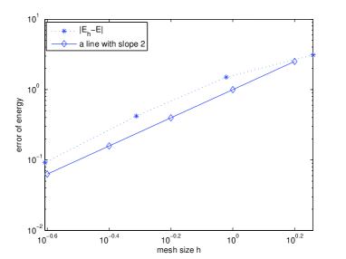
(a) Linear finite elements

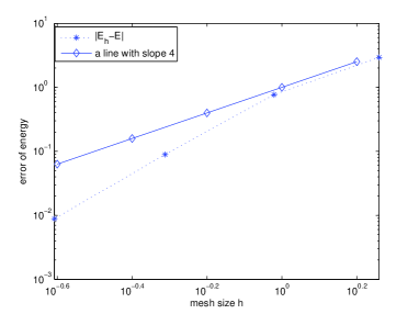
(b) Quadratic finite elements

Figure 5.1: $N_{2}$: errors of the ground state total energy

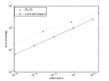
(a) Linear finite elements

(b) Quadratic finite elements

Figure 5.2: $C_{2}H_{4}$: errors of the ground state total energy

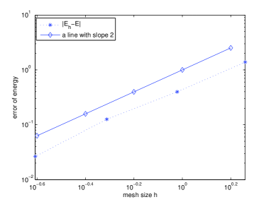
(a) Linear finite elements

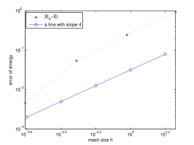
(b) Quadratic finite elements

Figure 5.3: $SiH_{4}$: errors of the ground state total energy

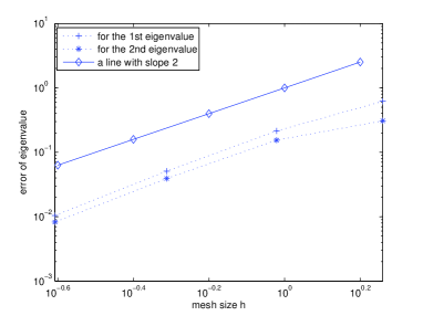
(a) Linear finite elements

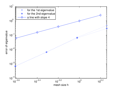
(b) Quadratic finite elements

Figure 5.4: $N_{2}$: errors of the first and second eigenvalues

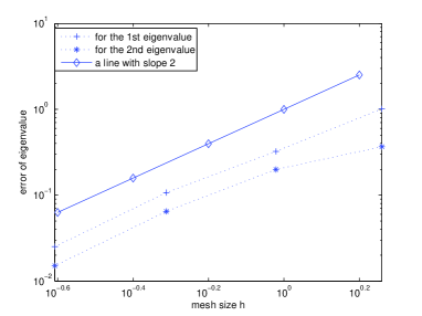
(a) Linear finite elements

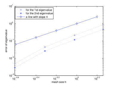
(b) Quadratic finite elements

Figure 5.5: $C_{2}H_{4}$: errors of the first and second eigenvalues

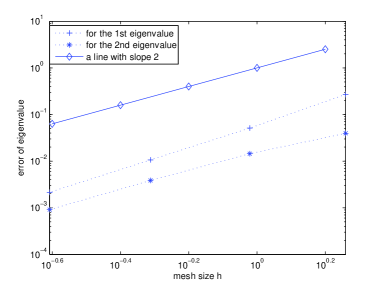
(a) Linear finite elements

(b) Quadratic finite elements

Figure 5.6: $SiH_{4}$: errors of the first and second eigenvalues

6 Concluding remarks

We have analyzed finite dimensional approximations of Kohn-Sham models. We have proved the convergence and shown the optimal a priori error estimates of finite dimensional approximations.

As we see, the ground state solutions oscillate near the nuclei [14, 17]. It is natural to apply adaptive finite element discretizations to carry out the electronic structure calculations. Indeed, it is our on-going work to study the convergence and complexity of adaptive finite element methods that will be addressed elsewhere.

Acknowledgements. The authors would like to thank Dr. Xiaoying Dai, Prof. Lihua Shen, and Dr. Dier Zhang for their stimulating discussions and fruitful cooperations on electronic structure computations that have motivated this work. The authors are grateful to Prof. Linbo Zhang and Dr. Tao Cui for their assistance on numerical computations and, to Mr. Zaikun Zhang for his discussions on the local uniqueness of the discrete solution.

References

• [1] S. Agmon, Lectures on the Exponential Decay of Solutions of Second-Order Elliptic Operators, Princeton University Press, Princeton, 1981.
• [2] A. Anantharaman and E. Cancès, Existence of minimizers for Kohn-Sham models in quantum chemistry, Ann. I. H. Poincaré-AN, 26 (2009), pp. 2425-2455.
• [3] T.A. Arias, Multiresolution analysis of electronic structure: Semicardinal and wavelet bases, Rev. Mod. Phys., 71 (1999), pp. 267-311.
• [4] G. Bao and A. Zhou, Analysis of finite dimensioanl approximations to a class of partial differential equaitons, Math. Meth. Appl. Sci., 27 (2004), pp. 2055-2066.
• [5] E. Cancès, R. Chakir, and Y. Maday, Numerical analysis of nonlinear eigenvalue problems, J. Sci. Comput., 45 (2010), pp. 90-117.
• [6] E. Cancès, R. Chakir, and Y. Maday, Numerical analysis of the planewave discretization of some orbital-free and Kohn-Sham models, arXiv:1003.1612, 2010.
• [7] C. Canuto, M.Y. Hussaini, A. Quarteroni, and T.A. Zang, Spectral Methods, Springer-Verlag, Berlin Heidelberg, 2007.
• [8] H. Chen, X. Gong, and A. Zhou, Numerical approximations of a nonlinear eigenvalue problem and applications to a density functional model, Math. Meth. Appl. Sci., 33 (2010), pp. 1723-1742.
• [9] H. Chen, L. He, and A. Zhou, Finite element approximations of nonlinear eigenvalue problems in quantum physics, Comput. Methods Appl. Mech. Engrg., 200 (2011), pp. 1846-1865.
• [10] H. Chen and A. Zhou, Orbital-free density functional theory for molecular structure calculations, Numer. Math. Theor. Meth. Appl., 1 (2008), pp. 1-28.
• [11] P.G. Ciarlet, The Finite Element Method for Elliptic Problems, North-Holland, 1978.
• [12] A. Edelman, T.A. Arias, and S.T. Smith, The geometry of algorithms with orthogonality constraints, SIAM J. Matrix Anal. Appl., 20 (1998), pp. 303-353.
• [13] L. Genovese, A. Neelov, S. Goedecker, T. Deutsch, S.A. Ghasemi, A. Willand, D. Caliste, O. Zilberberg, M. Rayson, A. Bergman, and R. Schneider, Daubechies wavelets as a basis set for density functional pseudopotential calculations, J. Chem. Phys., 129 (2008), pp. 014109-014112.
• [14] X. Gong, L. Shen, D. Zhang, and A. Zhou, Finite element approximations for Schrödinger equations with applications to electronic structure computations, J. Comput. Math., 26 (2008), pp. 310-323.
• [15] M. Hoffmann-Ostenhof, T. Hoffmann-Ostenhof, and T. Østergaard Sørensen, Electron wavefunctions and densities for atoms, Annales Henri Poincaré, 2 (2001), pp. 77-100.
• [16] P. Hohenberg and W. Kohn, Inhomogeneous Electron Gas, Phys. Rev. B, 136 (1964), pp. 864-871.
• [17] T. Kato, On the eigenfunctions of many-particle systems in quantum mechanics,Comm. Pure Appl. Math., 10 (1957), pp. 151-177.
• [18] W. Kohn and L.J. Sham, Self-consistent equations including exchange and correlation effects, Phys. Rev. A, 140 (1965), pp. 1133-1138.
• [19] B. Langwallner, C. Ortner, and E. Süli, Existence and convergence results for the Galerkin approximation of an electroniic density functional, $M^{3}AS$, doi: 10.1142/S021820251000491X.
• [20] C. Le Bris, Quelques problèmes mathématiques en chimie quanntique moléculaire, PhD thesis, Ècole Polytechnique, 1993.
• [21] C. Le Bris, ed., Handbook of Numerical Analysis, Vol. X. Special issue: Computational Chemistry, North-Holland, Amsterdam, 2003.
• [22] Y. Maday and G. Turinici, Error bars and quadratically convergent methods for the numerical simulation of the Hartree-Fock equations, Numer. Math., 94 (2000), pp. 739-770.
• [23] R.M. Martin, Electronic Structure: Basic Theory and Practical Method, Cambridge University Press, Cambridge, 2004.
• [24] M.C. Payne, M.P. Teter, D.C. Allan, T.A. Arias, and J.D. Joannopoulos, Iterative minimization techniques for ab-initio total-energy calculations: Molecular dynamics and conjugategradients, Rev. Mod. Phys., 64 (1992), pp. 1045-1097.
• [25] R.G. Parr and W.T. Yang, Density-Functional Theory of Atoms and Molecules, Clarendon Press, Oxford, 1994.
• [26] Y. Saad, J.R. Chelikowsky, and S.M. Shontz, Numerical methods for electronic structure calculations of materials, SIAM Review, 52 (2010), pp. 3-54.
• [27] R. Schneider, T. Rohwedder, A. Neelov, and J. Blauert, Direct minimization for calculating invariant subspaces in density functional computations of the electronic structure, J. Comput. Math., 27 (2009), pp. 360-387.
• [28] B. Simon, Schrödinger operators in the twentieth century, J. Math. Phys., 41 (2000), pp. 3523-3555.
• [29] P. Suryanarayana, V. Gavini, T. Blesgen, K. Bhattacharya, and M. Ortiz, Non-periodic finite-element formulation of Kohn-Sham density functional theory, J. Mech. Phys. Solid., 58 (2010), pp. 256-280.
• [30] N. Troullier and J.L. Martins, A straightforward method for generating soft transferable pseudopotentials, Solid State Comm., 74 (1990), pp. 613-616.
• [31] Y.A. Wang and E.A. Carter, Orbital-free kinetic-energy density functional theory, in: Theoretical Methods in Condensed Phase Chemistry (S. D. Schwartz, ed.), Kluwer, Dordrecht, 2000, pp. 117-184.
• [32] A. Zhou, An analysis of finite-dimensional approximations for the ground state solution of Bose-Einstein condensates, Nonlinearity, 17 (2004), pp. 541-550.
• [33] A. Zhou, Finite dimensional approximations for the electronic ground state solution of a molecular system, Math. Meth. Appl. Sci., 30 (2007), pp. 429-447.
• [34] A. Zhou, Multi-level adaptive corrections in finite dimensional approximations, J. Comput. Math., 28 (2010), pp. 45-54.