Existence and conditional energetic stability of three-dimensional fully localised solitary gravity-capillary water waves

Abstract

In this paper we show that the hydrodynamic problem for three-dimensional water waves with strong surface-tension effects admits a fully localised solitary wave which decays to the undisturbed state of the water in every horizontal direction. The proof is based upon the classical variational principle that a solitary wave of this type is a critical point of the energy, which is given in dimensionless coordinates by

$$\mathcal{E}(\eta,\phi)=\int_{{\mathbb{R}}^{2}}\left\{\frac{1}{2}\int_{0}^{1+\eta}(\phi_{x}^{2}+\phi_{y}^{2}+\phi_{z}^{2})\,\mathrm{d}y+\frac{1}{2}\eta^{2}+\beta[\sqrt{1+\eta_{x}^{2}+\eta_{z}^{2}}-1]\right\}\,\mathrm{d}x\,\mathrm{d}z,$$

subject to the constraint that the momentum

$$\mathcal{I}(\eta,\phi)=\int_{{\mathbb{R}}^{2}}\eta_{x}\phi|_{y=1+\eta}\,\mathrm{d}x\,\mathrm{d}z$$

is fixed; here $\{(x,y,z):x,z\in{\mathbb{R}},\ y\in(0,1+\eta(x,z))\}$ is the fluid domain, $\phi$ is the velocity potential and $\beta>1/3$ is the Bond number. These functionals are studied locally for $\eta$ in a neighbourhood of the origin in $H^{3}({\mathbb{R}}^{2})$.

We prove the existence of a minimiser of $\mathcal{E}$ subject to the constraint $\mathcal{I}=2\mu$, where $0<\mu\ll 1$. The existence of a small-amplitude solitary wave is thus assured, and since $\mathcal{E}$ and $\mathcal{I}$ are both conserved quantities a standard argument may be used to establish the stability of the set $D_{\mu}$ of minimisers as a whole. ‘Stability’ is however understood in a qualified sense due to the lack of a global well-posedness theory for three-dimensional water waves. We show that solutions to the evolutionary problem starting near $D_{\mu}$ remain close to $D_{\mu}$ in a suitably defined energy space over their interval of existence; they may however explode in finite time due to higher-order derivatives becoming unbounded.

1 Introduction

1.1 The hydrodynamic problem

The classical three-dimensional gravity-capillary water wave problem concerns the irrotational flow of a perfect fluid of unit density subject to the forces of gravity and surface tension. The fluid motion is described by the Euler equations in a domain bounded below by a rigid horizontal bottom $\{y=0\}$ and above by a free surface $\{y=h+\eta(x,z,t)\}$, where $h$ denotes the depth of the water in its undisturbed state and the function $\eta$ depends upon the two horizontal spatial directions $x$, $z$ and time $t$. In terms of an Eulerian velocity potential $\phi$, the mathematical problem is to solve Laplace’s equation

$$\phi_{xx}+\phi_{yy}+\phi_{zz}=0,\qquad\qquad 0<y<h+\eta$$

with boundary conditions

$$\phi_{y} = \parbox{284.52756pt}{$0$,}y=0,$$

$$\eta_{t} = \parbox{284.52756pt}{$\phi_{y}-\eta_{x}\phi_{x}-\eta_{z}\phi_{z}$,}y=h+\eta,$$

$$\phi_{t} = -\frac{1}{2}(\phi_{x}^{2}+\phi_{y}^{2}+\phi_{z}^{2})-g\eta$$

$$\parbox{284.52756pt}{$\displaystyle\qquad\mbox{}+\sigma\left[\frac{\eta_{x}}{\sqrt{1+\eta_{x}^{2}+\eta_{z}^{2}}}\right]_{x}+\sigma\left[\frac{\eta_{z}}{\sqrt{1+\eta_{x}^{2}+\eta_{z}^{2}}}\right]_{z}$,}y=h+\eta,$$

in which $g$ is the acceleration due to gravity and $\sigma>0$ is the coefficient of surface tension (see, for example, Stoker [28, §§1, 2.1]). Introducing the dimensionless variables

$$(x^{\prime},y^{\prime},z^{\prime})=\frac{1}{h}(x,y,z),\qquad t^{\prime}=\left(\frac{g}{h}\right)^{1/2},$$

$$\eta^{\prime}(x^{\prime},z^{\prime},t^{\prime})=\frac{1}{h}\eta(x,z,t),\qquad\phi^{\prime}(x^{\prime},y^{\prime},z^{\prime},t^{\prime})=\frac{1}{(gh)^{3/2}}\phi(x,y,z,t),$$

one obtains the equations

$$\phi_{xx}+\phi_{yy}+\phi_{zz}=0,\qquad\qquad 0<y<1+\eta$$ (1)

with boundary conditions

$$\phi_{y} = \parbox{284.52756pt}{$0$,}y=0,$$ (2)

$$\eta_{t} = \parbox{284.52756pt}{$\phi_{y}-\eta_{x}\phi_{x}-\eta_{z}\phi_{z}$,}y=1+\eta,$$ (3)

$$\phi_{t} = -\frac{1}{2}(\phi_{x}^{2}+\phi_{y}^{2}+\phi_{z}^{2})-\eta$$ (4)

$$\parbox{284.52756pt}{$\displaystyle\qquad\mbox{}+\beta\left[\frac{\eta_{x}}{\sqrt{1+\eta_{x}^{2}+\eta_{z}^{2}}}\right]_{x}+\beta\left[\frac{\eta_{z}}{\sqrt{1+\eta_{x}^{2}+\eta_{z}^{2}}}\right]_{z}$,}y=1+\eta,$$

where $\beta=\sigma/gh^{2}$ and the primes have been dropped for notational simplicity.

Steady waves are water waves which travel in a distinguished horizontal direction with constant speed and without change of shape; without loss of generality we assume that the waves propagate from right to left in the $x$-direction with speed $\nu$, so that $\eta(x,z,t)=\eta(x+\nu t,z)$ and $\phi(x,y,z,t)=\phi(x+\nu t,y,z)$. In this paper we study fully localised solitary waves, that is steady waves with the property that $\eta(x+\nu t,z)\rightarrow 0$ as $|(x+\nu t,z)|\rightarrow\infty$; in particular we consider the parameter regime $\beta>1/3$ corresponding to strong surface tension. Interest in this parameter regime stems from the celebrated Kadomtsev & Petviashvili (KP-I) equation (a model for long water waves with strong surface tension and a preferred direction of propagation), which admits a fully localised solitary-wave solution given by the explicit formula

$$u(x,z)=-8\frac{3-x^{2}+z^{2}}{(3+x^{2}+z^{2})^{2}}$$ (5)

in a frame of reference moving with the wave (see Ablowitz & Segur [1]); the variable $u$ is supposed to approximate the free surface of the water via the relationship

$$\eta(x,z)=\mu^{2}u\Bigg{(}\frac{\mu x}{2(\beta-1/3)^{1/2}},\mu^{2}z\Bigg{)}+O(\mu^{3}),$$ (6)

where $\mu$ is a small parameter associated with the weakly nonlinear scaling limit (see below).

Fully localised solitary-wave solutions to other models for three-dimensional surface-tension dominated flows have also been studied. Mathematical existence theories for generalised KP-I equations were given by Wang & Willem [29], de Bouard & Saut [15] and Pankov & Pflüger [25], and for the Benny-Luke equation (an isotropic version of the KP-I equation) by Pego & Quintero [27] (see Berger & Milewski [6] for numerical computations). The existence of a fully localised solitary-wave solution to (1)–(4) in this parameter regime was recently established rigorously by Groves & Sun [17] and computed numerically by Parau, Vanden-Broeck & Cooker [26] (see Figure 1). In the present paper we give an alternative, more natural existence theory. Groves & Sun work with Fourier-multiplier operators in $L^{p}$-based function spaces for $p>1$ (which require detailed analysis), and use a local reduction technique to reduce the problem to a single semilinear equation. On the other hand the present theory employs $L^{2}$-based function spaces and tackles the original hydrodynamic problem directly; furthermore, it yields information concerning the stability of the fully localised solitary wave.

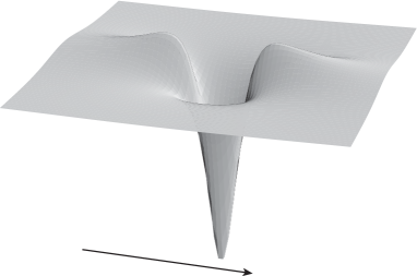
Figure 1: A fully localised solitary wave; the arrow shows the direction of wave propagation.

The conserved quantities

$$\mathcal{E}(\eta,\phi)=\int_{{\mathbb{R}}^{2}}\left\{\frac{1}{2}\int_{0}^{1+\eta}(\phi_{x}^{2}+\phi_{y}^{2}+\phi_{z}^{2})\,\mathrm{d}y+\frac{1}{2}\eta^{2}+\beta[\sqrt{1+\eta_{x}^{2}+\eta_{z}^{2}}-1]\right\}\,\mathrm{d}x\,\mathrm{d}z,$$

$$\mathcal{I}(\eta,\phi)=\int_{{\mathbb{R}}^{2}}\eta_{x}\phi|_{y=1+\eta}\,\mathrm{d}x\,\mathrm{d}z$$

of (1)–(4), which represent respectively the energy and momentum of a wave in the $x$-direction (see Benjamin & Olver [5]), are the key to our existence theory. A fully localised solitary wave is characterised as a critical point of the energy subject to the constraint of fixed momentum; it is therefore a critical point of the functional $\mathcal{E}-\nu\mathcal{I}$, where the Lagrange multiplier $\nu$ gives the speed of the wave. Furthermore, Benjamin [4] noted that constrained minimisers should be stable, and in this paper we construct an existence and stability theory for fully localised solitary waves using Benjamin’s principle.

1.2 Constrained minimisation and conditional energetic stability

The above formulation of the hydrodynamic problem has the disadvantage that it is posed in the a priori unknown domain $\{0<y<1+\eta(x,z,t)\}$. We overcome this difficulty using the Dirichlet-Neumann operator $G(\eta)$ introduced by Craig [12] and formally defined as follows. For fixed $\Phi=\Phi(x,z)$ solve the boundary-value problem

$$\parbox{170.71652pt}{$\phi_{xx}+\phi_{yy}+\phi_{zz}=0,$}0<y<1+\eta,$$

$$\parbox{170.71652pt}{$\phi=\Phi,$}y=1+\eta,$$

$$\parbox{170.71652pt}{$\phi_{y}=0,$}y=0$$

and define

$$G(\eta)\Phi = \sqrt{1+\eta_{x}^{2}+\eta_{z}^{2}}\left.\frac{\partial\phi}{\partial n}\right|_{y=1+\eta}$$

$$= \phi_{y}-\eta_{x}\phi_{x}-\eta_{z}\phi_{z}\Big{|}_{y=1+\eta}.$$

In terms of the variables $\eta$ and $\Phi$ the energy and momentum functionals are given by the convenient formulae

$$\mathcal{E}(\eta,\Phi)=\int_{{\mathbb{R}}^{2}}\left\{\frac{1}{2}\Phi G(\eta)\Phi+\frac{1}{2}\eta^{2}+\beta[\sqrt{1+\eta_{x}^{2}+\eta_{z}^{2}}-1]\right\}\,\mathrm{d}x\,\mathrm{d}z,$$ (7)

$$\mathcal{I}(\eta,\Phi)=\int_{{\mathbb{R}}^{2}}\eta_{x}\Phi\,\mathrm{d}x\,\mathrm{d}z,$$ (8)

and in this paper we study the problem of finding minimisers of $\mathcal{E}$ subject to the constraint

$$\mathcal{I}(\eta,\Phi)=2\mu,$$

where $\mu$ is a small positive number.

We begin our study in Section 2 by identifying function spaces in which equations (7), (8) define analytic functionals, using in particular the theory of analytic operators reported by Buffoni & Toland [10]. We take $\eta$ in a neighbourhood $U=B_{M}(0)$ of the origin in $H^{3}({\mathbb{R}}^{2})$, while the elements of the function space $H_{\star}^{1/2}({\mathbb{R}}^{2})$ for $\Phi$ are traces of potential functions in the fluid domain (see Section 2.1 for a precise definition). It follows from the following result, which is proved in Section 2.2, that $\mathcal{E}$ and $\mathcal{I}$ are smooth functionals $U\times H_{\star}^{1/2}({\mathbb{R}}^{2})\mapsto{\mathbb{R}}$.

Lemma 1.1

The mapping $W^{1,\infty}({\mathbb{R}}^{2})\rightarrow\mathcal{L}(H_{\star}^{1/2}({\mathbb{R}}^{2}),(H_{\star}^{1/2}({\mathbb{R}}^{2}))^{\prime})$ given by $\eta\mapsto(\Phi\mapsto G(\eta)\Phi)$ is analytic at the origin and $\Phi\rightarrow G(\eta)\Phi$ is an isomorphism $H_{\star}^{1/2}({\mathbb{R}}^{2})\rightarrow(H_{\star}^{1/2}({\mathbb{R}}^{2}))^{\prime}$ for each $\eta$ in a neighbourhood of the origin.

The above variational principle has been used by several authors in existence theories for three-dimensional steady water waves. Groves & Sun [17] obtained fully localised solitary waves as critical points of the functional $\mathcal{E}-\nu\mathcal{I}$, while Groves & Haragus [16] interpreted $\mathcal{E}-\nu\mathcal{I}$ as an action functional to derive a formulation of the hydrodynamic problem as an infinite-dimensional spatial Hamiltonian system with a rich solution set. Finally, Craig & Nicholls [13] developed an existence theory for doubly periodic steady waves as critical points of $\mathcal{E}$ on level sets of $\mathcal{I}$ (here the integrals over ${\mathbb{R}}^{2}$ are replaced with integrals over the periodic domain). These papers all use reduction methods to reduce the quasilinear problem under investigation to simpler semilinear or finite-dimensional problems.

In this paper we find constrained minimisers of $\mathcal{E}$ using a genuinely infinite-dimensional method. Our main existence result is stated in the following theorem (see Section 1.3 for an overview of the proof).

Theorem 1.2

• The set $D_{\mu}$ of minimisers of $\mathcal{E}$ over the set

  $$S_{\mu}=\{(\eta,\Phi)\in U\times H_{\star}^{1/2}({\mathbb{R}}^{2}):\mathcal{I}(\eta,\Phi)=2\mu\}$$

  is non-empty. The corresponding solitary waves are subcritical, that is their dimensionless speed is less than unity.

• Suppose that $\{(\eta_{n},\Phi_{n})\}\subset S_{\mu}$ is a minimising sequence for $\mathcal{E}$ with the property that

  $$\sup_{n\in{\mathbb{N}}}\|\eta_{n}\|_{3}<M.$$

  There exists a sequence $\{(x_{n},z_{n})\}\subset{\mathbb{R}}^{2}$ with the property that a subsequence of$\{\eta_{n}(x_{n}+\cdot,z_{n}+\cdot),\Phi_{n}(x_{n}+\cdot,z_{n}+\cdot)\}$ converges in $H^{r}({\mathbb{R}}^{2})\times H_{\star}^{1/2}({\mathbb{R}}^{2})$, $0\leq r<3$ to a function in $D_{\mu}$.

We discuss the stability of the set $D_{\mu}$ in Section 5. The usual informal interpretation of the statement that a set $X$ of solutions to an initial-value problem is ‘stable’ is that a solution which begins close to a solution in $X$ remains close to a solution in $X$ at all subsequent times. Implicit in this statement is the assumption that the initial-value problem is globally well-posed, that is every pair $(\eta_{0},\Phi_{0})$ in an appropriately chosen set is indeed the initial datum of a unique solution $t\mapsto(\eta(t),\Phi(t))$, $t\in[0,\infty)$. At present there is no global well-posedness theory for three-dimensional water waves, and we work instead under the following assumption (see Alazard, Burq & Zuly [3] for results of this kind).

(Well-posedness assumption) There exists a subset $S$ of $U\times H_{\star}^{1/2}({\mathbb{R}}^{2})$ with the following properties.

• The closure of $S\!\setminus\!D_{\mu}$ in $L^{2}({\mathbb{R}}^{2})$ has a non-empty intersection with $D_{\mu}$.

• For each $(\eta_{0},\Phi_{0})\in S$ there exists $T>0$ and a continuous function $t\mapsto(\eta(t),\Phi(t))\in U\times H_{\star}^{1/2}({\mathbb{R}}^{2})$, $t\in[0,T]$ such that $(\eta(0),\Phi(0))=(\eta_{0},\Phi_{0})$,

  $$\mathcal{E}(\eta(t),\Phi(t))=\mathcal{E}(\eta_{0},\Phi_{0}),\ \mathcal{I}(\eta(t),\Phi(t))=\mathcal{I}(\eta_{0},\Phi_{0}),\qquad t\in[0,T]$$

  and

  $$\sup_{t\in[0,T]}\|\eta(t)\|_{3}<M.$$

It is a general principle that the solution set of a constrained minimisation problem constitutes a stable set of solutions of the corresponding initial-value problem (e.g. see Cazenave & Lions [11] and de Bouard & Saut [14], Liu & Wang [21] for applications to generalised KP equations). Combining this general principle with our well-posedness assumption, we obtain the following stability result.

Theorem 1.3

Choose $r\in[0,3)$. For each $\varepsilon>0$ there exists $\delta>0$ such that

$$(\eta_{0},\Phi_{0})\in S,\ \mathrm{dist}((\eta_{0},\Phi_{0}),D_{\mu})<\delta\quad\Rightarrow\quad\mathrm{dist}((\eta(t),\Phi(t)),D_{\mu})<\varepsilon,$$

for $t\in[0,T]$, where ‘$\mathrm{dist}$’ denotes the distance in $H^{r}({\mathbb{R}}^{2})\times H_{\star}^{1/2}({\mathbb{R}}^{2})$.

This result is a statement of the conditional, energetic stability of the set $D_{\mu}$. Here energetic refers to the fact that the distance in the statement of stability is measured in the ‘energy space’ $H^{r}({\mathbb{R}}^{2})\times H_{\star}^{1/2}({\mathbb{R}}^{2})$, while conditional alludes to the well-posedness assumption. Note that the solution $t\mapsto(\eta(t),\Phi(t))$ may exist in a smaller space over the interval $[0,T]$, at each instant of which it remains close (in energy space) to a solution in $D_{\mu}$. Furthermore, Theorem 1.3 is a statement of the stability of the set of constrained minimisers $D_{\mu}$; establishing the uniqueness of the constrained minimiser would imply that $D_{\mu}$ consists of translations of a single solution, so that the statement that $D_{\mu}$ is stable is equivalent to classical orbital stability of this unique solution (Benjamin [4]). The phrase ‘conditional, energetic stability’ was introduced by Mielke [23] in his study of the stability of two-dimensional solitary water waves with strong surface tension using dynamical-systems methods and further developed in the context of variational methods for two-dimensional solitary waves by Buffoni [8, 9].

1.3 The minimisation problem

We tackle the problem of finding minimisers of $\mathcal{E}(\eta,\Phi)$ subject to the constraint $\mathcal{I}(\eta,\Phi)=2\mu$ in two steps.

1. Fix $\eta\neq 0$ and minimise $\mathcal{E}(\eta,\cdot)$ over $T_{\mu}=\{\Phi\in H^{1/2}_{\star}({\mathbb{R}}^{2}):\mathcal{I}(\eta,\Phi)=2\mu\}$. This problem (of minimising a quadratic functional over a linear manifold) admits a unique global minimiser $\Phi_{\eta}$.

2. Minimise $\mathcal{J}_{\mu}(\eta):=\mathcal{E}(\eta,\Phi_{\eta})$ over $\eta\in U\!\setminus\!\{0\}$. Because $\Phi_{\eta}$ minimises $\mathcal{E}(\eta,\cdot)$ over $T_{\mu}$ there exists a Lagrange multiplier $\lambda_{\eta}$ such that

   $$G(\eta)\Phi_{\eta}=\lambda_{\eta}\eta_{x},$$

   and straightforward calculations show that $\Phi_{\eta}=\lambda_{\eta}G(\eta)^{-1}\eta_{x}$, $\lambda_{\eta}=\mu/\mathcal{L}(\eta)$ and

   $$\mathcal{J}_{\mu}(\eta)=\mathcal{K}(\eta)+\frac{\mu^{2}}{\mathcal{L}(\eta)},$$ (9)

   where

   $$\mathcal{K}(\eta)=\int_{{\mathbb{R}}^{2}}\left\{\frac{1}{2}\eta^{2}+\beta\sqrt{1+\eta_{x}^{2}+\eta_{z}^{2}}-\beta\right\}\,\mathrm{d}x\,\mathrm{d}z,$$ (10)

   $$\mathcal{L}(\eta)=\frac{1}{2}\int_{{\mathbb{R}}^{2}}\eta_{x}G(\eta)^{-1}\eta_{x}\,\mathrm{d}x\,\mathrm{d}z.$$ (11)

   This computation also shows that the dimensionless speed of the solitary wave corresponding to a constrained minimiser of $\mathcal{E}(\eta,\Phi)$ is $\mu/\mathcal{L}(\eta)$.

The above two-step approach was introduced by Buffoni [7] in a corresponding theory for two-dimensional solitary waves. Buffoni used a conformal mapping to transform $\mathcal{K}$ and $\mathcal{L}$ into simpler functionals and hence greatly simplified the analysis necessary to show that $\mathcal{J}_{\mu}$ has a minimiser. Here we extend his method to our three-dimensional problem, working directly with the functionals as given above. In this respect we note that $\mathcal{K}$ is analytic at the origin in the Sobolev space $H^{r}({\mathbb{R}}^{2})$ for $r>2$, and it follows from the following result, which is proved in Section 2.2, that ${\mathcal{L}}$ is analytic at the origin in $H^{r}({\mathbb{R}}^{2})$ for $r>5/2$.

Lemma 1.4

Suppose that $s>1$. The operator $K(\cdot):H^{s+3/2}({\mathbb{R}}^{2})\rightarrow\mathcal{L}(H^{s+1}({\mathbb{R}}^{2}),H^{s}({\mathbb{R}}^{2}))$ given by the formula

$$K(\eta)=-\partial_{x}(G(\eta)^{-1}\partial_{x})$$

is analytic at the origin.

The above comments show that $\mathcal{J}_{\mu}$ is a smooth functional in a punctured neighbourhood of the origin in $H^{r}({\mathbb{R}}^{2})$ for $r>5/2$; we seek minimisers of $\mathcal{J}_{\mu}$ in the smaller space $H^{3}({\mathbb{R}}^{2})$, taking advantage of the fact that $H^{3}({\mathbb{R}}^{2})$ is locally compactly embedded in $H^{r}({\mathbb{R}}^{2})$ for $r\in[0,3)$. Our main result for $\mathcal{J}_{\mu}$, from which Theorem 1.2 is deduced in Section 5, is stated in the following theorem.

Theorem 1.5

There exists a neighbourhood $U=B_{M}(0)$ of the origin in $H^{3}({\mathbb{R}}^{2})$ with the following properties.

• The set of minimisers of $\mathcal{J}_{\mu}$ on $U\!\setminus\!\{0\}$ is non-empty.

• Suppose that $\{\eta_{n}\}$ is a minimising sequence for $\mathcal{J}_{\mu}$ over $U\!\setminus\!\{0\}$ which satisfies

  $$\sup_{n\in{\mathbb{N}}}\|\eta_{n}\|_{3}<M.$$

  There exists a sequence $\{(x_{n},z_{n})\}\subset{\mathbb{R}}^{2}$ with the property that a subsequence of$\{\eta_{n}(x_{n}+\cdot,z_{n}+\cdot)\}$ converges in $H^{r}({\mathbb{R}}^{2})$ for $r\in[0,3)$ to a critical point $\eta$ which minimises $\mathcal{J}_{\mu}$ on $U\!\setminus\!\{0\}$.

The theorem is proved by first reducing the first assertion to a special case of the second; in so doing one is immediately confronted by the unfavourable properties of the quadratic parts $\mathcal{K}_{2}$ and $\mathcal{L}_{2}$ of $\mathcal{K}$ and $\mathcal{L}$. The functionals are not coercive, in the sense that $(\mathcal{K}_{2})^{\frac{1}{2}}$ and $(\mathcal{L}_{2})^{\frac{1}{2}}$ are not bounded below by any constant multiple of the $H^{3}({\mathbb{R}}^{2})$-norm, and furthermore the functional

$$\mathcal{L}_{2}(\eta)=\frac{1}{2}\int_{{\mathbb{R}}^{2}}\frac{k_{1}^{2}}{|k|^{2}}|k|\coth|k||\hat{\eta}|^{2}\,\mathrm{d}k$$

is anisotropic and involves a Fourier multiplier which is not smooth at the origin. We proceed by introducing the penalised functional $\mathcal{J}_{\rho,\mu}:H^{3}({\mathbb{R}}^{2})\rightarrow{\mathbb{R}}\cup\{\infty\}$ defined by

$$\mathcal{J}_{\rho,\mu}(\eta)=\left\{\begin{array}[]{lll}\displaystyle\mathcal{K}(\eta)+\frac{\mu^{2}}{\mathcal{L}(\eta)}+\rho(\|\eta\|_{3}^{2}),&&u\in U\!\setminus\!\{0\},\\ \\ \infty,&&\eta\not\in U\!\setminus\!\{0\},\end{array}\right.$$

where $\rho:[0,M^{2})\rightarrow{\mathbb{R}}$ is a smooth, increasing ‘penalisation’ function which explodes to infinity as $t\uparrow M^{2}$ and vanishes for $0\leq t\leq\tilde{M}^{2}$; the number $\tilde{M}$ is chosen very close to $M$. This functional enjoys a degree of coercivity and has the advantage that a minimising sequence over $U\!\setminus\!\{0\}$ does not approach the boundary of $U$.

Minimising sequences $\{\eta_{n}\}$ for $\mathcal{J}_{\rho,\mu}$, which clearly satisfy $\sup\|\eta_{n}\|_{3}<M$, are studied in detail in Section 3 with the help of the concentration-compactness principle (Lions [19, 20]). The main difficulty here lies in discussing the consequences of ‘dichotomy’. On the one hand the functional ${\mathcal{L}}$ is nonlocal, so that a careful argument is required to show that $\eta_{n}$ splits into two parts in the usual fashion (see Lemma 3.10(iii) and Appendix D). On the other hand no a priori estimate is available to rule out ‘dichotomy’ at this stage; proceeding iteratively we find that minimising sequences can theoretically have profiles with infinitely many ‘lumps’. In particular we show that $\{\eta_{n}\}$ asymptotically lies in the region unaffected by the penalisation (Corollary 3.17) and construct a special minimising sequence $\{\tilde{\eta}_{n}\}$ for $\mathcal{J}_{\rho,\mu}$ which lies in a neighbourhood of the origin with radius $O(\mu^{\frac{1}{2}})$ in $H^{3}({\mathbb{R}}^{2})$ and satisfies $\|\mathcal{J}^{\prime}_{\mu}(\tilde{\eta}_{n})\|_{1}\rightarrow 0$ as $n\rightarrow\infty$ (Section 3.4). The fact that the construction is independent of the choice of $\tilde{M}$ allows us to conclude that $\{\tilde{\eta}_{n}\}$ is also a minimising sequence for $\mathcal{J}_{\mu}$ over $U\!\setminus\!\{0\}$.

The special minimising sequence $\{\tilde{\eta}_{n}\}$ is used in Section 4 to establish the strict sub-additivity property

$$c_{\mu_{1}+\mu_{2}}<c_{\mu_{1}}+c_{\mu_{2}},\qquad\mu_{1},\mu_{2}>0$$

of the infimum $c_{\mu}$ of $\mathcal{J}_{\mu}$ over $U\!\setminus\!\{0\}$. An argument given by Buffoni [7] shows how this property follows from the fact that the function

$$a\mapsto a^{-\frac{5}{2}}\mathcal{M}_{a^{2}\mu}(a\eta_{n}),\qquad a\in[1,2],$$ (12)

is decreasing and strictly negative, where $\{\eta_{n}\}$ is a minimising sequence for $\mathcal{J}_{\mu}$ over $U\!\setminus\!\{0\}$ and

$$\mathcal{M}_{\mu}(\eta):=\mathcal{J}_{\mu}(\eta)-\mathcal{K}_{2}(\eta)-\frac{\mu^{2}}{\mathcal{L}_{2}(\eta)}$$

is the ‘nonlinear’ part of $\mathcal{J}_{\mu}(\eta)$. The function (12) would clearly have the required property if $\mathcal{M}_{\mu}(\eta_{n})$ were homogeneous cubic and negative; we therefore proceed by approximating $\mathcal{M}_{\mu}(\eta_{n})$ with an expression of this kind.

Using the fact that every minimising sequence $\{\eta_{n}\}$ satisfies $\mathcal{L}_{2}(\eta_{n})$, $\mathcal{L}(\eta_{n})\geq c\mu$,$\mathcal{M}_{\mu}(\eta_{n})\leq-c\mu^{3}$, one finds that the ‘cubic’ part of $\mathcal{M}_{\mu}(\eta_{n})$ is $-(\mu/\mathcal{L}_{2}(\eta_{n}))^{2}\mathcal{L}_{3}(\eta_{n})$ and that $\mathcal{M}_{\mu}(\eta_{n})$ can be approximated by a cubic, negative expression provided that all other terms in $\mathcal{M}_{\mu}(\eta_{n})$ are $o(\mu^{3})$. The straightforward estimate $\|\eta_{n}\|_{3}^{2}=O(\mu)$ does not suffice for this purpose (the ‘quartic’ part of $\mathcal{M}_{\mu}(\eta_{n})$ would for example be merely $O(\mu^{2})$). Motivated by the expectation that a critical point of $\mathcal{J}_{\mu}$, and hence the minimising sequence $\{\tilde{\eta}_{n}\}$, should have the KP-I length scales, we prove that $|{\mskip-2.0mu}|{\mskip-2.0mu}|\tilde{\eta}_{n}|{\mskip-2.0mu}|{\mskip-2.0mu}|_{\alpha}^{2}=O(\mu)$ for each $\alpha<1$, where

$$|{\mskip-2.0mu}|{\mskip-2.0mu}|\eta|{\mskip-2.0mu}|{\mskip-2.0mu}|_{\alpha}^{2}:=\int_{{\mathbb{R}}^{2}}\left(1+\mu^{-6\alpha}|k|^{6}+\mu^{-4\alpha}\frac{k_{2}^{4}}{|k|^{4}}\right)|\hat{\eta}|^{2}\,\mathrm{d}k;$$

the third term in this expression takes account of the anisotropy and the non-smooth Fourier multiplier in the functional $\mathcal{L}_{2}$. The $L^{2}({\mathbb{R}}^{2})$-norm of each derivative of $\tilde{\eta}_{n}$ thus gains a factor of $\mu^{\alpha}$, and this fact allows one to obtain better estimates for the parts $\mathcal{K}_{k}$ and $\mathcal{L}_{k}$ of $\mathcal{K}$ and $\mathcal{L}$ which are homogeneous of degree $k$ and hence confirm that $\mathcal{M}_{\mu}(\tilde{\eta}_{n})=-(\mu/\mathcal{L}_{2}(\tilde{\eta}_{n}))^{2}\mathcal{L}_{3}(\tilde{\eta}_{n})+o(\mu^{3})$.

Theorem 1.5(ii) is established in Section 5. Its proof, which relies upon the strict-subadditivity of $c_{\mu}$ and estimates for general minimising sequences derived in Section 3, is now a straightforward application of the concentration-compactness principle.

2 The functional-analytic setting

2.1 The Neumann-Dirichlet operator

Our first task is to find suitable function spaces for the functionals $\mathcal{E}$ and $\mathcal{I}$ defined in equations (7), (8) and introduce rigorous definitions of the Dirichlet-Neumann operator $G(\eta)$ and its inverse. Since the functional $\mathcal{J}_{\mu}$ to be minimised involves $G(\eta)^{-1}$ (see equation (9)) we begin with the formal definition of this Neumann-Dirichlet operator $N(\eta)$: for fixed $\xi=\xi(x,z)$ solve the boundary-value problem

$$\parbox{170.71652pt}{$\phi_{xx}+\phi_{yy}+\phi_{zz}=0,$}0<y<1+\eta,$$ (13)

$$\parbox{170.71652pt}{$\phi_{y}-\eta_{x}\phi_{x}-\eta_{z}\phi_{z}=\xi,$}y=1+\eta,$$ (14)

$$\parbox{170.71652pt}{$\phi_{y}=0,$}y=0$$ (15)

and define

$$N(\eta)\xi=\phi|_{y=1+\eta}.$$

We study this boundary-value problem by transforming it to an equivalent problem in a fixed domain (cf. Nicholls & Reitich [24]). The change of variable

$$y^{\prime}=\frac{y}{1+\eta},\qquad u(x,y^{\prime},z)=\phi(x,y,z)$$

transforms the variable domain $\{0<y<1+\eta(x,z)\}$ into the slab $\Sigma=\{(x,y^{\prime},z)\in{\mathbb{R}}\times(0,1)\times{\mathbb{R}}\}$ and the boundary-value problem (13)–(15) into

$$\parbox{256.0748pt}{$u_{xx}+u_{yy}+u_{zz}=\partial_{x}F_{1}+\partial_{z}F_{2}+\partial_{y}F_{3},$}0<y<1,$$ (16)

$$\parbox{256.0748pt}{$u_{y}=F_{3}+\xi,$}y=1,$$ (17)

$$\parbox{256.0748pt}{$u_{y}=0,$}y=0,$$ (18)

where

$$F_{1} = -\eta u_{x}+y\eta_{x}u_{y},$$

$$F_{2} = -\eta u_{z}+y\eta_{z}u_{y},$$

$$F_{3} = \frac{\eta u_{y}}{1+\eta}+y\eta_{x}u_{x}+y\eta_{z}u_{z}-\frac{y^{2}}{1+\eta}\eta_{x}^{2}u_{y}-\frac{y^{2}}{1+\eta}\eta_{z}^{2}u_{y}$$

and we have again dropped the primes for notational simplicity; the Neumann-Dirichlet operator is given by

$$N(\eta)\xi=u|_{y=1}.$$

The next step is to develop a convenient theory for weak solutions of the boundary-value problem (16)–(18). The observation that solutions of this problem are unique only up to additive constants leads us to introduce the completion $H_{\star}^{1}(\Sigma)$ of

$$\SS(\Sigma,{\mathbb{R}})=\{u\in C^{\infty}(\bar{\Sigma}):|(x,z)|^{m}|\partial_{x}^{\alpha_{1}}\partial_{z}^{\alpha_{2}}u|\mbox{ is bounded for all }m,\alpha_{1},\alpha_{2}\in{\mathbb{N}}_{0}\}$$

with respect to the norm

$$\|u\|_{\star}^{2}:=\int_{\Sigma}(u_{x}^{2}+u_{y}^{2}+u_{z}^{2})\,\mathrm{d}y\,\mathrm{d}x\,\mathrm{d}z$$

as an appropriate function space for $u$. The corresponding space for the trace $u|_{y=1}$ is the completion $H_{\star}^{1/2}({\mathbb{R}}^{2})$ of the inner product space $X_{\star}^{1/2}({\mathbb{R}}^{2})$ constructed by equipping the Schwartz class $\SS({\mathbb{R}}^{2},{\mathbb{R}})$ with the norm

$$\|\eta\|_{\star,1/2}^{2}:=\int_{{\mathbb{R}}^{2}}(1+|k|^{2})^{-\frac{1}{2}}|k|^{2}|\hat{\eta}|^{2}\,\mathrm{d}k,$$

where $\hat{\eta}$ denotes the Fourier transform of $\eta$; its dual $(H_{\star}^{1/2}({\mathbb{R}}^{2}))^{\prime}$ is the space

$$(X_{\star}^{1/2}({\mathbb{R}}^{2}))^{\prime}=\Big{\{}u\in\SS^{\prime}({\mathbb{R}}^{2},{\mathbb{R}}):\sup\{|(u,\eta)|:\eta\in X_{\star}^{1/2}({\mathbb{R}}^{2}),\,\|\eta\|_{\star,1/2}<1\}<\infty\Big{\}},$$

where $\SS^{\prime}({\mathbb{R}}^{2},{\mathbb{R}})$ is the class of two-dimensional, real-valued, tempered distributions. A more convenient description of $(H_{\star}^{1/2}({\mathbb{R}}^{2}))^{\prime}$ is however available.

Proposition 2.1

Let $H_{\star}^{-1/2}({\mathbb{R}}^{2})$ be the completion of the inner product space $X_{\star}^{-1/2}({\mathbb{R}}^{2})$ constructed by equipping $\bar{\SS}({\mathbb{R}}^{2},{\mathbb{R}})$ with the norm

$$\|\eta\|_{\star,-1/2}^{2}:=\int_{{\mathbb{R}}^{2}}(1+|k|^{2})^{\frac{1}{2}}|k|^{-2}|\hat{\eta}|^{2}\,\mathrm{d}k,$$

where $\bar{\SS}({\mathbb{R}}^{2},{\mathbb{R}})$ is the subclass of $\SS({\mathbb{R}}^{2},{\mathbb{R}})$ consisting of functions with zero mean. The space $H_{\star}^{-1/2}({\mathbb{R}}^{2})$ can be identified with $(H_{\star}^{1/2}({\mathbb{R}}^{2}))^{\prime}$.

Proof. In the usual manner we identify $u\in X_{\star}^{-1/2}({\mathbb{R}}^{2})$ with the distribution

$$(u,\eta)=\int_{{\mathbb{R}}^{2}}u\eta\,\mathrm{d}x\,\mathrm{d}z,$$

which belongs to $(H_{\star}^{1/2}({\mathbb{R}}^{2}))^{\prime}$ and satisfies $\|u\|_{(H_{\star}^{1/2}({\mathbb{R}}^{2}))^{\prime}}=\|u\|_{\star,-1/2}$; it follows that $H_{\star}^{-1/2}({\mathbb{R}}^{2})$ is a subspace of $(H_{\star}^{1/2}({\mathbb{R}}^{2}))^{\prime}$.

We now demonstrate that $\eta=0$ is the only function $\eta\in X_{\star}^{1/2}({\mathbb{R}}^{2})$ with the property that $(u,\eta)=0$ for all $u\in X_{\star}^{-1/2}({\mathbb{R}}^{2})$; this fact implies that $X_{\star}^{-1/2}({\mathbb{R}}^{2})$ is dense in $(X_{\star}^{1/2}({\mathbb{R}}^{2}))^{\prime}=(H_{\star}^{1/2}({\mathbb{R}}^{2}))^{\prime}$ and yields the required result. To this end, we note that the stated property of $\eta$ asserts in particular that $(\eta_{0},\eta)=0$, where $\eta_{0}\in X_{\star}^{-1/2}({\mathbb{R}}^{2})$ is given by the formula $\hat{\eta}_{0}=(1+|k|^{2})^{-\frac{1}{2}}|k|^{2}\hat{\eta}$, and the only solution of the equation

$$0=(\eta_{0},\eta)=\int_{{\mathbb{R}}^{2}}(1+|k|^{2})^{-\frac{1}{2}}|k|^{2}|\hat{\eta}|^{2}\,\mathrm{d}k$$

is indeed $\eta=0$. (The Fourier transform maps $\bar{\SS}({\mathbb{R}}^{2},{\mathbb{R}})$ bijectively onto the subclass

$$\SS_{0}({\mathbb{R}}^{2},{\mathbb{C}})=\{\eta\in\SS({\mathbb{R}}^{2},{\mathbb{C}}):\eta(0)=0,\ \eta(-k)=\overline{\eta(k)}\mbox{ for all }k\in{\mathbb{R}}^{2}\}$$

of $\SS({\mathbb{R}}^{2},{\mathbb{C}})$.) $\Box$

The following proposition, which is proved by elementary estimates, confirms the required relationship between $H_{\star}^{1}(\Sigma)$ and $H_{\star}^{1/2}({\mathbb{R}}^{2})$.

Proposition 2.2

The trace map $u\mapsto u|_{y=1}$ defines a continuous operator $H_{\star}^{1}(\Sigma)\rightarrow H_{\star}^{1/2}({\mathbb{R}}^{2})$ and has a continuous right inverse $H_{\star}^{1/2}({\mathbb{R}}^{2})\rightarrow H_{\star}^{1}(\Sigma)$.

Finally, let us take $\eta\in B_{1/2}(0)\subset W^{1,\infty}({\mathbb{R}}^{2})$, so that the estimates

$$\|F_{j}\|_{0}\leq c\|\eta\|_{1,\infty}^{2}\|u\|_{\star},\qquad j=1,2,3$$ (19)

imply $F_{1}$, $F_{2}$, $F_{3}\in L^{2}(\Sigma)$. It is then a straightforward matter to define and prove the existence of a unique weak solution to (16)–(18).

Definition 2.3

Suppose that $\xi\in H_{\star}^{-1/2}({\mathbb{R}}^{2})$ and $\eta\in B_{M}(0)\subset W^{1,\infty}({\mathbb{R}}^{2})$. A weak solution of (16)–(18) is a function $u\in H_{\star}^{1}(\Sigma)$ which satisfies

$$\int_{\Sigma}(u_{x}w_{x}+u_{y}w_{y}+u_{z}w_{z})\,\mathrm{d}x\,\mathrm{d}y\,\mathrm{d}z$$

$$=\int_{\Sigma}(F_{1}w_{x}+F_{2}w_{z}+F_{3}w_{y})\,\mathrm{d}x\,\mathrm{d}y\,\mathrm{d}z+\int_{{\mathbb{R}}^{2}}\xi w|_{y=1}\,\mathrm{d}x\,\mathrm{d}z$$

for all $w\in H_{\star}^{1}(\Sigma)$.

Lemma 2.4

For each $\xi\in H_{\star}^{-1/2}({\mathbb{R}}^{2})$ and $\eta\in B_{1/2}(0)\subset W^{1,\infty}({\mathbb{R}}^{2})$ the boundary-value problem (16)–(18) has a unique weak solution $u\in H_{\star}^{1}(\Sigma)$.

Proof. The existence of a unique weak solution $u\in H_{\star}^{1}(\Sigma)$ of (16)–(18) follows from the estimates (19),

$$\int_{{\mathbb{R}}^{2}}\xi u|_{y=1}\,\mathrm{d}x\,\mathrm{d}z\ \leq\ \|\xi\|_{\star,-1/2}\|u|_{y=1}\|_{\star,1/2}\ \leq\ c\|\xi\|_{\star,-1/2}\|u\|_{\star}$$

and the Lax-Milgram lemma. $\Box$

We conclude with a rigorous definition of the Neumann-Dirichlet operator.

Definition 2.5

The Neumann-Dirichlet operator for the boundary-value problem (16)–(18) is the bounded linear operator $N(\eta):H_{\star}^{-1/2}({\mathbb{R}}^{2})\rightarrow H_{\star}^{1/2}({\mathbb{R}}^{2})$ defined by

$$N(\eta)\xi=u|_{y=1},$$

where $u\in H_{\star}^{1}(\Sigma)$ is the unique weak solution of (16)–(18).

Remark 2.6

Observe that

$$\int_{{\mathbb{R}}^{2}}\xi N(\eta)\xi\,\mathrm{d}x\,\mathrm{d}z$$

$$= \int_{{\mathbb{R}}^{2}}(\phi_{y}-\eta_{x}\phi_{x}-\eta_{z}\phi_{z})\phi|_{y=\eta}\,\mathrm{d}x\,\mathrm{d}z$$

$$= \int_{\{y=1+\eta\}}\phi\frac{\partial\phi}{\partial n}\,\mathrm{d}x\,\mathrm{d}z$$

$$= \int_{\{0<y<1+\eta\}}\Big{(}\phi_{x}^{2}+\phi_{y}^{2}+\phi_{z}^{2}\Big{)}\,\mathrm{d}x\,\mathrm{d}y\,\mathrm{d}z$$

$$= \int_{\Sigma}\left(\!\left(u_{x}-\frac{y\eta_{x}u_{y}}{1+\eta}\right)^{\!\!2}+\frac{u_{y}^{2}}{(1+\eta)^{2}}+\left(u_{z}-\frac{y\eta_{z}u_{y}}{1+\eta}\right)^{\!\!2}\right)(1+\eta)\,\mathrm{d}x\,\mathrm{d}y\,\mathrm{d}z.$$

2.2 Analyticity of the Neumann-Dirichlet operator

In this section we establish that $N(\eta)$ is an analytic function of $\eta$ in the above function spaces and examine some consequences of this fact. Let us begin by recording the definition of analyticity given by Buffoni & Toland [10, Definition 4.3.1] together with a useful fact concerning multiplication of multilinear operators.

Definition 2.7

Let $X$ and $Y$ be Banach spaces, $U$ be a non-empty, open subset of $X$ and $\mathcal{L}_{\mathrm{s}}^{k}(X,Y)$ be the space of bounded, $k$-linear symmetric operators $X^{k}\rightarrow Y$ with norm

$$|{\mskip-2.0mu}|{\mskip-2.0mu}|m|{\mskip-2.0mu}|{\mskip-2.0mu}|:=\inf\{c:\|m(\{f\}^{(k)})\|_{Y}\leq c\|f\|_{X}^{k}\mbox{ \rm{for all} }f\in X\}.$$

A function $F:U\rightarrow Y$ is analytic at a point $x_{0}\in U$ if there exist real numbers $\delta,r>0$ and a sequence $\{m_{k}\}$, where $m_{k}\in\mathcal{L}_{\mathrm{s}}^{k}(X,Y)$, $k=0,1,2,\ldots$, with the properties that

$$F(x)=\sum_{k=0}^{\infty}m_{k}(\{x-x_{0}\}^{(k)}),\qquad x\in B_{\delta}(x_{0})$$

and

$$\sup_{k\geq 0}r^{k}|{\mskip-2.0mu}|{\mskip-2.0mu}|m_{k}|{\mskip-2.0mu}|{\mskip-2.0mu}|<\infty.$$

Remark 2.8

Let $X$, $Y_{1}$ and $Y_{2}$ be Banach spaces. Suppose that $m_{1}\in\mathcal{L}_{\mathrm{s}}^{k_{1}}(X,Y_{1})$, $m_{2}\in\mathcal{L}_{\mathrm{s}}^{k_{2}}(X,Y_{1})$ and that the operation of pointwise multiplication defines a bounded bilinear operator $Y_{1}\times Y_{2}\rightarrow Y$. There exists a unique $m_{3}\in\mathcal{L}_{\mathrm{s}}^{k_{1}+k_{2}}(X,Y)$ with the property that

$$m_{1}(\{f\}^{(k_{1})})m_{2}(\{f\}^{(k_{2})})=m_{3}(\{f\}^{(k_{1}+k_{2})}).$$

Our first task is to establish the following theorem.

Theorem 2.9

The mapping $W^{1,\infty}({\mathbb{R}}^{2})\rightarrow\mathcal{L}(H_{\star}^{-1/2}({\mathbb{R}}^{2}),H_{\star}^{1/2}({\mathbb{R}}^{2}))$ given by $\eta\mapsto(\xi\mapsto u|_{y=1})$, where $u\in H_{\star}^{1}(\Sigma)$ is the unique weak solution of (16)–(18), is analytic at the origin.

We prove Theorem 2.9 using a modification of a method due to Nicholls & Reitich [24]. Let us seek a solution of (16)–(18) of the form

$$u(x,y,z)=\sum_{n=0}^{\infty}u^{n}(x,y,z),$$ (20)

where $u^{n}$ is a function of $\eta$ and $\xi$ which is homogeneous of degree $n$ in $\eta$ and linear in $\xi$. Substituting this Ansatz into the equations, one finds that

$$\parbox{170.71652pt}{$u_{xx}^{0}+u_{yy}^{0}+u_{zz}^{0}=0,$}0<y<1,$$ (21)

$$\parbox{170.71652pt}{$u_{y}^{0}=\xi,$}y=1,$$ (22)

$$\parbox{170.71652pt}{$u_{y}^{0}=0,$}y=0$$ (23)

and

$$\parbox{256.0748pt}{$u_{xx}^{n}+u_{yy}^{n}+u_{zz}^{n}=\partial_{x}F_{1}^{n}+\partial_{z}F_{2}^{n}+\partial_{y}F_{3}^{n},$}0<y<1,$$ (24)

$$\parbox{256.0748pt}{$u_{y}^{n}=F_{3}^{n},$}y=1,$$ (25)

$$\parbox{256.0748pt}{$u_{y}^{n}=0,$}y=0$$ (26)

for $n=1,2,3,\ldots$, where

$$F_{1}^{n} = -\eta u_{x}^{n-1}+y\eta_{x}u_{y}^{n-1},$$ (27)

$$F_{2}^{n} = -\eta u_{z}^{n-1}+y\eta_{z}u_{y}^{n-1},$$ (28)

$$F_{3}^{n} = \eta\sum_{\ell=0}^{n-1}(-\eta)^{\ell}u_{y}^{n-1-\ell}+y\eta_{x}u_{x}^{n-1}+y\eta_{z}u_{z}^{n-1}-y^{2}(\eta_{x}^{2}+\eta_{z}^{2})\sum_{\ell=0}^{n-2}(-\eta)^{\ell}u_{y}^{n-2-\ell}.$$ (29)

Definition 2.10

• Suppose that $\xi\in H_{\star}^{-1/2}({\mathbb{R}}^{2})$. A weak solution of (21)–(23) is a function $u^{0}\in H_{\star}^{1}(\Sigma)$ which satisfies

  $$\int_{\Sigma}(u_{x}^{0}w_{x}+u_{y}^{0}w_{y}+u_{z}^{0}w_{z})\,\mathrm{d}x\,\mathrm{d}y\,\mathrm{d}z=\int_{S}\xi w|_{y=1}\,\mathrm{d}x\,\mathrm{d}z$$ (30)

  for all $w\in H_{\star}^{1}(\Sigma)$. (The existence and uniqueness of a weak solution $u^{0}$, which satisfies the estimate

  $$\|u^{0}\|_{\star}\leq C_{1}\|\xi\|_{\star,-1/2},$$ (31)

  follows from the Lax-Milgram lemma.)

• Suppose that $F_{1}^{n}$, $F_{2}^{n}$, $F_{3}^{n}\in L^{2}(\Sigma)$. A weak solution of (24)–(26) is a function $u^{n}\in H_{\star}^{1}(\Sigma)$ which satisfies

  $$\int_{\Sigma}(u_{x}^{n}w_{x}+u_{y}^{n}w_{y}+u_{z}^{n}w_{z})\,\mathrm{d}x\,\mathrm{d}y\,\mathrm{d}z=\int_{\Sigma}(F_{1}^{n}w_{x}+F_{2}^{n}w_{z}+F_{3}^{n}w_{y})\,\mathrm{d}x\,\mathrm{d}y\,\mathrm{d}z$$ (32)

  for all $w\in H_{\star}^{1}(\Sigma)$. (The existence and uniqueness of a weak solution $u^{n}$, which satisfies the estimate

  $$\|u^{n}\|_{\star}\leq C_{2}(\|F_{1}^{n}\|_{0}+\|F_{2}^{n}\|_{0}+\|F_{3}^{n}\|_{0}),$$ (33)

  follows from the Lax-Milgram lemma.)

The next step is to compute the weak solutions $u^{0}$ and $u^{n}$, $n=1,2,\ldots$ of the boundary-value problems (21)–(23) and (24)–(26) inductively. In this fashion we obtain a sequence $\{m^{n}\}_{n=0}^{\infty}$ of $n$-linear symmetric operators such that

$$u^{n}=m^{n}(\{\eta\}^{(n)}).$$

Lemma 2.11

Suppose there exist $m^{k}\in\mathcal{L}_{\mathrm{s}}^{k}(W^{1,\infty}({\mathbb{R}}^{2}),H_{\star}^{1}(\Sigma))$ and constants $C_{1}>0$, $B_{1}>2$ such that

$$u^{k}=m^{k}(\{\eta\}^{(k)}),\qquad|{\mskip-2.0mu}|{\mskip-2.0mu}|m_{j}^{k}|{\mskip-2.0mu}|{\mskip-2.0mu}|\leq C_{1}B_{1}^{k}\|\xi\|_{\star,-1/2}$$

for $k=0,\ldots,n-1$.

There exist $\tilde{m}_{1}^{n}$, $\tilde{m}_{2}^{n}$, $\tilde{m}_{3}^{n}\in\mathcal{L}_{\mathrm{s}}^{n}(W^{1,\infty}({\mathbb{R}}^{2}),L^{2}(\Sigma))$ and a constant $C_{3}>0$ such that

$$F_{j}^{n}=\tilde{m}_{j}^{n}(\{\eta\}^{(n)}),\quad|{\mskip-2.0mu}|{\mskip-2.0mu}|\tilde{m}_{j}^{n}|{\mskip-2.0mu}|{\mskip-2.0mu}|\leq C_{1}C_{3}B_{1}^{n-1}\|\xi\|_{\star,-1/2},\qquad j=1,2,3.$$

Proof. The existence of $\tilde{m}_{1}^{n}$, $\tilde{m}_{2}^{n}$, $\tilde{m}_{3}^{n}$ follows from the formulae (27)–(29) defining $F_{1}^{n}$, $F_{2}^{n}$, $F_{3}^{n}$ and Remark 2.8.

Observe that

$$\|F_{1}^{n}\|_{0}\ \leq\ \|\eta\|_{1,\infty}(\|u_{x}^{n-1}\|_{0}+\|u_{y}^{n-1}\|_{0})\ \leq\ 2C_{1}B_{1}^{n-1}\|\xi\|_{\star,-1/2}\|\eta\|_{1,\infty}^{n},$$

$$\|F_{2}^{n}\|_{0}\ \leq\ \|\eta\|_{1,\infty}(\|u_{z}^{n-1}\|_{0}+\|u_{y}^{n-1}\|_{0})\ \leq\ 2C_{1}B_{1}^{n-1}\|\xi\|_{\star,-1/2}\|\eta\|_{1,\infty}^{n}.$$

A similar calculation yields

$$\|F_{3}^{n}\|_{0} \leq 2C_{1}B_{1}^{n-1}\|\xi\|_{\star,-1/2}\|\eta\|_{1,\infty}^{n}$$

$$\qquad\mbox{}+C_{1}\|\xi\|_{\star,-1/2}\|\eta\|_{1,\infty}^{n}\sum_{\ell=0}^{n-1}B_{1}^{n-1-\ell}+2C_{1}\|\xi\|_{\star,-1/2}\|\eta\|_{1,\infty}^{n}\sum_{\ell=0}^{n-2}B_{1}^{n-2-\ell},$$

and estimating

$$\sum_{\ell=0}^{n-1}B_{1}^{n-1-\ell}\ =\ B_{1}^{n-1}\sum_{\ell=0}^{n-1}B_{1}^{-\ell}\ <\ B_{1}^{n-1}\sum_{\ell=0}^{n-1}\left(\frac{1}{2}\right)^{\!\!\ell}\ <\ B_{1}^{n-1}\sum_{\ell=0}^{\infty}\left(\frac{1}{2}\right)^{\!\!\ell}\ =\ 2B_{1}^{n-1},$$

$$\sum_{\ell=0}^{n-2}B_{1}^{n-2-\ell}\ <\ 2B_{1}^{n-2}\ <\ B_{1}^{n-1},$$

we find that

$$\|F_{3}^{n}\|_{0}\leq 6C_{1}B_{1}^{n-1}\|\xi\|_{\star,-1/2}\|\eta\|_{1,\infty}^{n}.$$

Theorem 2.12

There exist $m^{n}\in\mathcal{L}_{\mathrm{s}}^{n}(W^{1,\infty}({\mathbb{R}}^{2}),H_{\star}^{1}(\Sigma))$ and constants $C_{1}>0$, $B>1$ with the properties that

$$u^{n}=m^{n}(\{\eta\}^{(n)}),\qquad|{\mskip-2.0mu}|{\mskip-2.0mu}|m^{n}|{\mskip-2.0mu}|{\mskip-2.0mu}|\leq C_{1}B_{1}^{n}\|\xi\|_{\star,-1/2}$$

for $n=0,1,2,\ldots$.

Proof. This result is obtained by mathematical induction. The base step ($n=0$) follows from estimate (31). Suppose the result is true for all $k<n$. The existence of $m^{n}$ follows from Lemma 2.11 and the fact that $u^{n}\in H_{\star}^{1}(\Sigma)$ is a bounded linear function of $F_{1}^{n}$, $F_{2}^{n}$, $F_{3}^{n}\in L^{2}(\Sigma)$; using the estimate (33), one finds that

$$\|u\|_{\star}\ \leq\ 3C_{2}C_{1}C_{3}B_{1}^{n-1}\|\xi\|_{\star,-1/2}\|\eta\|_{1,\infty}^{n}\ \leq\ C_{1}B_{1}^{n}\|\xi\|_{\star,-1/2}\|\eta\|_{1,\infty}^{n},$$

upon choosing $B_{1}>3C_{2}C_{3}$. $\Box$

Corollary 2.13

The mapping $W^{1,\infty}({\mathbb{R}}^{2})\rightarrow\mathcal{L}(H_{\star}^{-1/2}({\mathbb{R}}^{2}),H_{\star}^{1}(\Sigma))$ given by $\eta\mapsto(\xi\mapsto u)$, where $u\in H_{\star}^{1}(\Sigma)$ is the unique weak solution of (16)–(18), is analytic at the origin.

Proof. According to Definition 2.7 the mapping $W^{1,\infty}({\mathbb{R}}^{2})\rightarrow\mathcal{L}(H_{\star}^{-1/2}({\mathbb{R}}^{2}),H_{\star}^{1}(\Sigma))$ given by $\eta\mapsto(\xi\mapsto u)$, where $u$ is defined by (20), (21)–(23) and (24)–(26), is analytic at the origin.

It remains to verify that $u$ is a weak solution of (16)–(18). The facts that

$$\sum_{n=0}^{N}u_{x}^{n}\rightarrow u_{x},\quad\sum_{n=0}^{N}u_{y}^{n}\rightarrow u_{y},\quad\sum_{n=0}^{N}u_{z}^{n}\rightarrow u_{z}$$

in $L^{2}(\Sigma)$ and hence that

$$\sum_{n=1}^{N}F_{j}^{n}\rightarrow F_{j},\quad j=1,2,3$$

in $L^{2}(\Sigma)$ imply that

$$\int_{\Sigma}\left\{\left(\textstyle\sum_{n=0}^{N}u_{x}^{n}\right)w_{x}+\left(\textstyle\sum_{n=0}^{N}u_{y}^{n}\right)w_{y}+\left(\textstyle\sum_{n=0}^{N}u_{z}^{n}\right)w_{z}\right\}\,\mathrm{d}x\,\mathrm{d}y\,\mathrm{d}z$$

$$\rightarrow\int_{\Sigma}(u_{x}w_{x}+u_{y}w_{y}+u_{z}w_{2})\,\mathrm{d}x\,\mathrm{d}y\,\mathrm{d}z\hskip 71.13188pt$$

and

$$\int_{\Sigma}\left\{\left(\textstyle\sum_{n=1}^{N}F_{1}^{n}\right)w_{x}+\left(\textstyle\sum_{n=1}^{N}F_{2}^{n}\right)w_{y}+\left(\textstyle\sum_{n=1}^{N}F_{3}^{n}\right)w_{z}\right\}\,\mathrm{d}x\,\mathrm{d}y\,\mathrm{d}z$$

$$\rightarrow\int_{\Sigma}(F_{1}w_{x}+F_{2}w_{y}+F_{3}w_{2})\,\mathrm{d}x\,\mathrm{d}y\,\mathrm{d}z\hskip 71.13188pt$$

for each $w\in H_{\star}^{1}(\Sigma)$. It follows from these results, equations (30), (32) and the uniqueness of limits that $u$ is a weak solution of (16)–(18). $\Box$

Theorem 2.9 is a direct consequence of the above corollary. Using this result and the continuity of the trace operator $H_{\star}^{1}(\Sigma)\rightarrow H_{\star}^{1/2}({\mathbb{R}}^{2})$, we find that the Neumann-Dirichlet operator $W^{1,\infty}({\mathbb{R}}^{2})\rightarrow\mathcal{L}(H_{\star}^{-1/2}({\mathbb{R}}^{2}),H_{\star}^{1/2}({\mathbb{R}}^{2}))$ given by $\eta\mapsto(\xi\mapsto u|_{y=1})$ is analytic at the origin; its series representation is given by

$$N(\eta)=\sum_{n=0}^{\infty}N^{n}(\eta),$$

where $N^{n}(\eta)\xi=u^{n}|_{y=1}$.

The next step is to show that the Neumann-Dirichlet operator is invertible and that its inverse is also an analytic function of $\eta$ at the origin in $W^{1,\infty}({\mathbb{R}}^{2})$.

Proposition 2.14

The operator $N(0):H_{\star}^{-1/2}({\mathbb{R}}^{2})\rightarrow H_{\star}^{1/2}({\mathbb{R}}^{2})$ is an isomorphism and the norm

$$\xi\mapsto\left(\int_{{\mathbb{R}}^{2}}\xi N(0)\xi\,\mathrm{d}x\,\mathrm{d}z\right)^{\!\!\frac{1}{2}}$$

is equivalent to the usual norm on $H_{\star}^{-1/2}({\mathbb{R}}^{2})$.

Proof. Observe that $N(0)$ admits the representation

$$N(0)\xi=\mathcal{F}^{-1}\left[\frac{\coth|k|}{|k|}\hat{\xi}\right]$$

as a Fourier-multiplier operator. Using the estimate

$$c(1+|k|^{2})^{\frac{1}{2}}\ \leq\ |k|\coth|k|\ \leq\ c(1+|k|^{2})^{\frac{1}{2}}$$

one finds that

$$c\|\xi\|_{\star,-1/2}^{2}\ \leq\ \int_{{\mathbb{R}}^{2}}\xi N(0)\xi\,\mathrm{d}x\,\mathrm{d}z\leq c\|\xi\|_{\star,-1/2}^{2},$$ (34)

which establishes the second assertion; the first assertion follows from the first inequality in the above estimate. $\Box$

Corollary 2.15

The estimate

$$c\|\xi\|_{\star,-1/2}^{2}\ \leq\ \int_{{\mathbb{R}}^{2}}\xi N(\eta)\xi\,\mathrm{d}x\,\mathrm{d}z\leq c\|\xi\|_{\star,-1/2}^{2}$$

holds for each $\eta\in B_{M}(0)\subset W^{1,\infty}({\mathbb{R}}^{2})$. In particular, the operator $N(\eta):H_{\star}^{-1/2}({\mathbb{R}}^{2})\rightarrow H_{\star}^{1/2}({\mathbb{R}}^{2})$ is an isomorphism and the norm

$$\xi\mapsto\left(\int_{{\mathbb{R}}^{2}}\xi N(\eta)\xi\,\mathrm{d}x\,\mathrm{d}z\right)^{\!\!\frac{1}{2}}$$

is equivalent to the usual norm on $H_{\star}^{-1/2}({\mathbb{R}}^{2})$.

Proof. It follows from the analyticity of $N(\cdot):W^{1,\infty}({\mathbb{R}}^{2})\rightarrow\mathcal{L}(H_{\star}^{-1/2}({\mathbb{R}}^{2}),H_{\star}^{1/2}({\mathbb{R}}^{2}))$ at the origin that

$$\|N(\eta)-N(0)\|_{\mathcal{L}(H_{\star}^{-1/2}({\mathbb{R}}^{2}),H_{\star}^{1/2}({\mathbb{R}}^{2}))}\ \leq\ c\|\eta\|_{1,\infty}\ \leq\ cM$$

and hence that

$$\left|\int_{{\mathbb{R}}^{2}}\xi N(\eta)\xi\,\mathrm{d}x\,\mathrm{d}z-\int_{{\mathbb{R}}^{2}}\xi N(0)\xi\,\mathrm{d}x\,\mathrm{d}z\right|\leq cM\|\xi\|_{\star,-1/2}^{2}.$$

The result is obtained by choosing $M$ sufficiently small and combining the above estimate with (34). $\Box$

Definition 2.16

The Dirichlet-Neumann operator for the boundary-value problem (16)–(18) is the bounded linear operator $G(\eta):H_{\star}^{1/2}({\mathbb{R}}^{2})\rightarrow H_{\star}^{-1/2}({\mathbb{R}}^{2})$ defined by $G(\eta)\Phi=N(\eta)^{-1}\Phi$.

Lemma 2.17

The Dirichlet-Neumann operator $G(\cdot):W^{1,\infty}({\mathbb{R}}^{2})\rightarrow\mathcal{L}(H_{\star}^{1/2}({\mathbb{R}}^{2}),H_{\star}^{-1/2}({\mathbb{R}}^{2}))$ is analytic at the origin and the estimate

$$c\|\Phi\|_{\star,1/2}^{2}\ \leq\ \int_{{\mathbb{R}}^{2}}\Phi G(\eta)\Phi\,\mathrm{d}x\,\mathrm{d}z\leq c\|\Phi\|_{\star,1/2}^{2}$$

holds for each $\eta\in B_{M}(0)\subset W^{1,\infty}({\mathbb{R}}^{2})$.

Proof. Define $F_{1}:\mathcal{L}(H_{\star}^{1/2}({\mathbb{R}}^{2}),H_{\star}^{-1/2}({\mathbb{R}}^{2}))\times B_{M}(0)\rightarrow\mathcal{L}(H_{\star}^{1/2}({\mathbb{R}}^{2}),H_{\star}^{1/2}({\mathbb{R}}^{2}))$ and $F_{2}:\mathcal{L}(H_{\star}^{1/2}({\mathbb{R}}^{2}),H_{\star}^{-1/2}({\mathbb{R}}^{2}))\times B_{M}(0)\rightarrow\mathcal{L}(H_{\star}^{-1/2}({\mathbb{R}}^{2}),H_{\star}^{-1/2}({\mathbb{R}}^{2}))$ by the formulae

$$F_{1}(A,\eta)=N(\eta)A-I_{1},\qquad F_{2}(A,\eta)=AN(\eta)-I_{2},$$

where $I_{1}$ and $I_{2}$ are the identity operators on respectively $H_{\star}^{1/2}({\mathbb{R}}^{2})$ and $H_{\star}^{-1/2}({\mathbb{R}}^{2})$. It follows from the implicit function theorem that the equations

$$F_{1}(A,\eta)=0,\qquad F_{2}(A,\eta)=0$$

have unique solutions $A_{1}=A_{1}(\eta)$, $A_{2}=A_{2}(\eta)$ which are analytic at the origin; by uniqueness we deduce that $A_{1}(\eta)=A_{2}(\eta)=G(\eta)$.

The inequality is obtained by writing $\xi=G(\eta)\Phi$ in the inequality given in Corollary 2.15. $\Box$

2.3 The operator $K$

Observe that the formula (11) defining $\mathcal{L}$ may be written as

$$\mathcal{L}(\eta)=\frac{1}{2}\int_{{\mathbb{R}}^{2}}\eta K(\eta)\eta\,\mathrm{d}x\,\mathrm{d}z,$$ (35)

where

$$K(\eta)=-\partial_{x}(N(\eta)\partial_{x}),$$

and we now study this operator in detail. Our first result is obtained from the material presented in Section 2.2.

Corollary 2.18

The operator $K(\cdot):W^{1,\infty}({\mathbb{R}}^{2})\rightarrow\mathcal{L}(H^{1/2}({\mathbb{R}}^{2}),H^{-1/2}({\mathbb{R}}^{2}))$ is analytic at the origin.

Proof. This result follows from the definition of $K$ and the continuity of the operators $\partial_{x}:H^{1/2}({\mathbb{R}}^{2})\rightarrow H_{\star}^{-1/2}({\mathbb{R}}^{2})$ and $\partial_{x}:H_{\star}^{1/2}({\mathbb{R}}^{2})\rightarrow H^{-1/2}({\mathbb{R}}^{2})$. $\Box$

In the remainder of this section we establish the following result concerning the analyticity of $K$ in the Sobolev spaces

$$H^{r}({\mathbb{R}}^{2})=\left\{\eta\in(\SS({\mathbb{R}}^{2},{\mathbb{R}}))^{\prime}:\|\eta\|_{r}^{2}:=\int_{{\mathbb{R}}^{2}}(1+|k|^{2})^{r}|\hat{\eta}(k)|^{2}\,\mathrm{d}k<\infty\right\}.$$

Theorem 2.19

Suppose that $s>1$. The operator $K(\cdot):H^{s+3/2}({\mathbb{R}}^{2})\rightarrow\mathcal{L}(H^{s+1}({\mathbb{R}}^{2}),H^{s}({\mathbb{R}}^{2}))$ is analytic at the origin.

The first step in the proof of this theorem is to establish additional regularity of the weak solutions $u^{0}$ and $u^{n}$, $n=1,2,\ldots$ of the boundary-value problems (21)–(23) and (24)–(26). This task is accomplished in the Propositions 2.20 and 2.21 below; the proof of the latter is given in Appendix A. We work in the function spaces $(H^{r}(\Sigma),\|\cdot\|_{r})$; for $r\notin{\mathbb{N}}_{0}$ the space is defined by interpolation in the sense of Lions & Magenes [18] (see also Adams & Fournier [2, §7.57]).

Proposition 2.20

For each $r\geq 0$ the weak solution to the boundary-value problem (21)–(23) with $\xi=\zeta_{x}$ satisfies

$$\|u_{x}^{0}\|_{r}\,\|u_{y}^{0}\|_{r},\,\|u_{z}^{0}\|_{r}\leq C_{4}\|\zeta\|_{r+1/2}.$$

Proof. The Fourier transform of the weak solution $u^{0}$ of (21)–(23) is given by

$$\hat{u}^{0}=\frac{\cosh|k|y}{|k|\sinh|k|}\hat{\xi}.$$

Using this formula with $\xi=\zeta_{x}$, we find that

$$\hat{u}_{y}^{0}=\frac{\mathrm{i}k_{1}\sinh|k|y}{\sinh|k|}\hat{\zeta},\quad\hat{u}_{x}^{0}=\frac{-k_{1}^{2}\cosh|k|y}{|k|\sinh|k|}\hat{\zeta},\quad\hat{u}_{z}^{0}=\frac{-k_{1}k_{2}\cosh|k|y}{|k|\sinh|k|}\hat{\zeta},$$ (36)

whereby

$$\Big{|}\mathcal{F}[\partial_{x}^{\alpha_{1}}\partial_{y}^{\alpha_{2}}\partial_{z}^{\alpha_{3}}\left\{\begin{array}[]{c}u_{y}^{0}\\ u_{x}^{0}\\ u_{z}^{0}\end{array}\right\}\Big{|}\leq\frac{|k|^{\alpha_{1}+\alpha_{2}+\alpha_{3}+1}}{\sinh|k|}\left\{\begin{array}[]{c}\sinh|k|y\\ \cosh|k|y\end{array}\right\}|\hat{\zeta}|,$$

where we have estimated $|k_{1}|,|k_{2}|\leq|k|$. It follows that

$$\left\|\mathcal{F}[\partial_{x}^{\alpha_{1}}\partial_{y}^{\alpha_{2}}\partial_{z}^{\alpha_{3}}\left\{\begin{array}[]{c}u_{y}^{0}\\ u_{x}^{0}\\ u_{z}^{0}\end{array}\right\}\right\|_{0}^{2} = \int_{\Sigma}\Big{|}\mathcal{F}[\partial_{x}^{\alpha_{1}}\partial_{y}^{\alpha_{2}}\partial_{z}^{\alpha_{3}}\left\{\begin{array}[]{c}u_{y}^{0}\\ u_{x}^{0}\\ u_{z}^{0}\end{array}\right\}\Big{|}^{2}\,\mathrm{d}y\,\mathrm{d}x\,\mathrm{d}z$$

$$= \int_{{\mathbb{R}}^{2}}\frac{|k|^{2(\alpha_{1}+\alpha_{2}+\alpha_{3}+1)}}{\sinh^{2}|k|}\left\{\pm\frac{1}{2}+\frac{\sinh 2|k|}{4|k|}\right\}|\hat{\zeta}|^{2}\,\mathrm{d}x\,\mathrm{d}z$$

$$\leq \int_{{\mathbb{R}}^{2}}(1+|k|^{2})^{\alpha_{1}+\alpha_{2}+\alpha_{3}+1/2}|\hat{\zeta}|^{2}\,\mathrm{d}x\,\mathrm{d}z$$

$$= c\|\zeta\|_{\alpha_{1}+\alpha_{2}+\alpha_{3}+1/2}^{2},$$

in which the estimates

$$\frac{|k|^{2}}{\sinh^{2}|k|}\left(-\frac{1}{2}+\frac{\sinh 2|k|}{4|k|}\right)\leq c|k|,\qquad\frac{|k|^{2}}{\sinh^{2}|k|}\left(\frac{1}{2}+\frac{\sinh 2|k|}{4|k|}\right)\leq c(1+|k|^{2})^{\frac{1}{2}}$$

have been used.

The above calculations show that

$$\left\|\left\{\begin{array}[]{c}u_{y}^{0}\\ u_{x}^{0}\\ u_{z}^{0}\end{array}\right\}\right\|_{n}^{2}\ =\!\!\!\!\sum_{0\leq\alpha_{1}+\alpha_{2}+\alpha_{3}\leq n}\left\|\partial_{x}^{\alpha_{1}}\partial_{y}^{\alpha_{2}}\partial_{z}^{\alpha_{3}}\left\{\begin{array}[]{c}u_{y}^{0}\\ u_{x}^{0}\\ u_{z}^{0}\end{array}\right\}\right\|_{n}^{2}\ \leq\ c\!\!\!\!\sum_{0\leq\alpha_{1}+\alpha_{2}+\alpha_{3}\leq n}\|\zeta\|_{n+1/2}^{2}$$

for $n\in{\mathbb{N}}_{0}$, and it follows by interpolation that

$$\left\|\left\{\begin{array}[]{c}u_{y}^{0}\\ u_{x}^{0}\\ u_{z}^{0}\end{array}\right\}\right\|_{r}\leq c\|\zeta\|_{r+1/2},\qquad r\geq 0.$$

Proposition 2.21

Suppose that $F_{1}^{n}$, $F_{2}^{n}$, $F_{3}^{n}\in H^{r}(\Sigma)$ for $r\geq 0$. The weak solution to the boundary-value problem (24)–(26) satisfies

$$\|u^{n}_{x}\|_{r},\,\|u^{n}_{y}\|_{r},\,\|u^{n}_{z}\|_{r}\leq C_{5}(\|F_{1}^{n}\|_{r}+\|F_{2}^{n}\|_{r}+\|F_{3}^{n}\|_{r}).$$

Lemma 2.22

Suppose that $s>1$ and there exist $m_{1}^{k}$, $m_{2}^{k}$, $m_{3}^{k}\in\mathcal{L}_{\mathrm{s}}^{k}(H^{s+3/2}({\mathbb{R}}^{2}),H^{s+1/2}(\Sigma))$ and constants $C_{4}>0$, $B_{2}>2$ such that

$$u_{x}^{k}=m_{1}^{k}(\{\eta\}^{(k)}),\quad u_{y}^{k}=m_{2}^{k}(\{\eta\}^{(k)}),\quad u_{z}^{k}=m_{3}^{k}(\{\eta\}^{(k)})$$

and

$$|{\mskip-2.0mu}|{\mskip-2.0mu}|m_{j}^{k}|{\mskip-2.0mu}|{\mskip-2.0mu}|\leq C_{4}B_{2}^{k}\|\zeta\|_{s+1},\qquad j=1,2,3$$

for $k=0,\ldots,n-1$.

There exist $m_{1}^{n}$, $m_{2}^{n}$, $m_{3}^{n}\in\mathcal{L}_{\mathrm{s}}^{n}(H^{s+3/2}({\mathbb{R}}^{2}),H^{s+1/2}(\Sigma))$ and a constant $C_{6}>0$ such that

$$F_{j}^{n}=m_{j}^{n}(\{\eta\}^{(n)}),\quad|{\mskip-2.0mu}|{\mskip-2.0mu}|m_{j}^{n}|{\mskip-2.0mu}|{\mskip-2.0mu}|\leq C_{4}C_{6}B_{2}^{n-1}\|\zeta\|_{s+1},\qquad j=1,2,3.$$

Proof. This result is proved inductively in the same way as Theorem 2.12. The base step follows from Proposition 2.20, while the inductive step is treated according to the strategy of Lemma 2.11. Using the inequalities

$$\|w_{1}w_{2}\|_{s+1/2}\leq c_{s}\|w_{1}\|_{s+1/2}\|w_{2}\|_{s+1/2},\qquad s>1$$

and

$$\|w\|_{H^{r}(\Sigma)}\leq\|w\|_{H^{r}({\mathbb{R}}^{2})},\qquad w=w(x,z),\qquad r\geq 0,$$

one finds that

$$\|F_{1}^{n}\|_{s+1/2} \leq c_{s}\|\eta\|_{s+1/2}\|u_{x}^{n-1}\|_{s+1/2}+c_{s}^{2}\|y\|_{s+1/2}\|\eta_{x}\|_{s+1/2}\|u_{y}^{n-1}\|_{s+1/2}$$

$$\leq C_{4}\|\zeta\|_{s+1}(c_{s}+c_{s}^{2}\|y\|_{s+1/2})B_{2}^{n-1}\|\eta\|_{s+3/2}^{n}$$

and similarly

$$\|F_{2}^{n}\|_{s+1/2} \leq C_{4}\|\zeta\|_{s+1}(c_{s}+c_{s}^{2}\|y\|_{s+1/2})B_{2}^{n-1}\|\eta\|_{s+3/2}^{n},$$

$$\|F_{3}^{n}\|_{s+1/2} \leq 2C_{4}c_{s}^{2}\|y\|_{s+1/2}\|\zeta\|_{s+1}B_{2}^{n-1}\|\eta\|_{s+3/2}^{n}+C_{4}c_{s}\|\zeta\|_{s+1}\|\eta\|_{s+3/2}^{n}\sum_{\ell=0}^{n-1}c_{s}^{\ell}B_{2}^{n-1-\ell}$$

$$\qquad\mbox{}+2C_{4}c_{s}^{4}\|y\|_{s+1/2}^{2}\|\zeta\|_{s+1}\|\eta\|_{s+3/2}^{n}\sum_{\ell=0}^{n-2}c_{s}^{\ell}B_{2}^{n-2-\ell};$$

the inductive step is completed by choosing $B_{2}>\max\{2c_{s},6C_{5}(c_{s}+c_{s}^{2}\|y\|_{s+1/2}+c_{s}^{4}\|y\|_{s+1/2}^{2})\}$ and using Proposition 2.21. $\Box$

Corollary 2.23

For each $s>1$ the mappings $H^{s+3/2}({\mathbb{R}}^{2})\rightarrow\mathcal{L}(H^{s+1}({\mathbb{R}}^{2}),H^{s+1/2}(\Sigma))$ given by $\eta\mapsto(\zeta\mapsto u_{x})$, $\eta\mapsto(\zeta\mapsto u_{y})$ and $\eta\mapsto(\zeta\mapsto u_{z})$, where $u$ is the weak solution of (16)–(18) with $\xi=\zeta_{x}$, are analytic at the origin.

Theorem 2.19 follows from the above corollary, the definition $K:\eta\mapsto(\zeta\mapsto-u_{x}|_{y=1})$ and the continuity of the trace operator $H^{s+1/2}(\Sigma)\rightarrow H^{s}({\mathbb{R}}^{2})$ for $s>1$. We write

$$K(\eta)=\sum_{n=0}^{\infty}K^{n}(\eta),$$

where $K^{n}(\eta)\zeta=-u_{x}^{n}|_{y=1}$ and observe that

$$K^{0}\zeta=\mathcal{F}^{-1}\left[\frac{k_{1}^{2}}{|k|^{2}}|k|\coth|k|\hat{\zeta}\right]$$

(see (36)).

Remark 2.24

A straightforward modification of the above analysis yields analogous results (with the same function spaces) for the operators

$$L(\eta):=-\partial_{z}(N(\eta)\partial_{x}),\qquad M(\eta):=-\partial_{z}(N(\eta)\partial_{z});$$

we write

$$L(\eta)=\sum_{n=0}^{\infty}L^{n}(\eta),\qquad M(\eta)=\sum_{n=0}^{\infty}M^{n}(\eta)$$

and note that

$$L^{0}\zeta=\mathcal{F}^{-1}\left[\frac{k_{1}k_{2}}{|k|^{2}}|k|\coth|k|\hat{\zeta}\right],\qquad M^{0}\zeta=\mathcal{F}^{-1}\left[\frac{k_{2}^{2}}{|k|^{2}}|k|\coth|k|\hat{\zeta}\right].$$

2.4 The functionals $\mathcal{K}$, $\mathcal{L}$ and $\mathcal{J}_{\mu}$

The following lemma formally states the analyticity property of $\mathcal{K}$ (examine the explicit formula for $\mathcal{K}$) and $\mathcal{L}$ (see Theorem 2.19). In particular this result implies that $\mathcal{K},\mathcal{L}$ belong to the class $C^{\infty}(U,{\mathbb{R}})$ and that equation (9) defines an operator $\mathcal{J}_{\mu}\in C^{\infty}(U\!\setminus\!\{0\},{\mathbb{R}})$, where $U=B_{M}(0)\subset H^{3}({\mathbb{R}}^{2})$ and $M$ is chosen sufficiently small.

Lemma 2.25

Equations (10), (11) define functionals $\mathcal{K}:H^{s+1}({\mathbb{R}}^{2})\rightarrow{\mathbb{R}}$, $\mathcal{L}:H^{s+3/2}({\mathbb{R}}^{2})\rightarrow{\mathbb{R}}$ for $s>1$ which are analytic at the origin and satisfy $\mathcal{K}(0)=\mathcal{L}(0)=0$.

The following results state further useful properties of the operators $\mathcal{K}$ and $\mathcal{L}$.

Proposition 2.26

The functionals $\mathcal{K}$ and $\mathcal{L}$ satisfy

$$\mathcal{K}(\eta)\geq c\|\eta\|_{1}^{2},\qquad\mathcal{L}(\eta)\geq c\|\eta_{x}\|_{\star,-1/2}^{2}$$

for each $\eta\in U$.

Proof. Using the estimates

$$\eta_{x}^{2},\eta_{z}^{2}\ \leq\ \|\eta\|_{1,\infty}^{2}\ \leq\ c\|\eta\|_{3}^{2}\ \leq\ cM^{2},\qquad\eta\in U$$

and choosing $M$ small enough so that $(1+\eta_{x}^{2}+\eta_{z}^{2})^{1/2}\leq 2$, we find that

$$\mathcal{K}(\eta) = \int_{{\mathbb{R}}^{2}}\left\{\frac{\beta(\eta_{x}^{2}+\eta_{z}^{2})}{1+(1+\eta_{x}^{2}+\eta_{z}^{2})^{1/2}}+\frac{\eta^{2}}{2}\right\}\,\mathrm{d}x\,\mathrm{d}z$$

$$\geq \frac{1}{3}\int_{{\mathbb{R}}^{2}}\left\{\beta\eta_{x}^{2}+\beta\eta_{z}^{2}+\eta^{2}\right\}\,\mathrm{d}x\,\mathrm{d}z$$

$$\geq c\|\eta\|_{1}^{2},$$

and furthermore

$$\mathcal{L}(\eta)\ =\ \frac{1}{2}\int_{{\mathbb{R}}^{2}}\eta_{x}G(\eta)^{-1}\eta_{x}\,\mathrm{d}x\,\mathrm{d}z\ \geq\ c\|\eta_{x}\|_{\star,-1/2}^{2},\qquad\eta\in U$$

(see Corollary 2.15). $\Box$

Lemma 2.27

The gradients $\mathcal{K}^{\prime}(\eta)$ and $\mathcal{L}^{\prime}(\eta)$ in $L^{2}({\mathbb{R}}^{2})$ exist for each $\eta\in U$ and are given by the formulae

$$\mathcal{K}^{\prime}(\eta) = -\left(\frac{\beta\eta_{x}}{\sqrt{1+\eta_{x}^{2}+\eta_{z}^{2}}}\right)_{\!\!x}-\left(\frac{\beta\eta_{z}}{\sqrt{1+\eta_{x}^{2}+\eta_{z}^{2}}}\right)_{\!\!z}+\eta,$$

$$\mathcal{L}^{\prime}(\eta) = -\frac{1}{2}(u_{x}^{2}+u_{z}^{2})+\frac{u_{y}^{2}}{2(1+\eta)^{2}}(\eta_{x}^{2}+\eta_{z}^{2})+\frac{u_{y}^{2}}{2(1+\eta)^{2}}\Bigg{|}_{y=1}+K(\eta)\eta,$$

where $u$ is the weak solution of the boundary-value problem (16)–(18) with $\xi=\eta_{x}$. These formulae define functions $\mathcal{K}^{\prime}:H^{3}({\mathbb{R}}^{2})\rightarrow H^{1}({\mathbb{R}}^{2})$, $\mathcal{L}^{\prime}:H^{s+3/2}({\mathbb{R}}^{2})\rightarrow H^{s}({\mathbb{R}}^{2})$ for $s>1$ which are analytic at the origin and satisfy $\mathcal{K}^{\prime}(0)=\mathcal{L}^{\prime}(0)=0$.

Proof. Differentiating the formulae (10) and

$$\mathcal{L}(\eta)=\frac{1}{2}\int_{\Sigma}\left(\!\left(u_{x}-\frac{y\eta_{x}u_{y}}{1+\eta}\right)^{\!\!2}+\frac{u_{y}^{2}}{(1+\eta)^{2}}+\left(u_{z}-\frac{y\eta_{z}u_{y}}{1+\eta}\right)^{\!\!2}\right)(1+\eta)\,\mathrm{d}x\,\mathrm{d}y\,\mathrm{d}z$$

(see Remark 2.6), one finds that

$$\mathrm{d}\mathcal{K}[\eta](\omega)=\int_{{\mathbb{R}}^{2}}\left\{\frac{\beta\eta_{x}\omega_{x}}{\sqrt{1+\eta_{x}^{2}+\eta_{z}^{2}}}+\frac{\beta\eta_{z}\omega_{z}}{\sqrt{1+\eta_{x}^{2}+\eta_{z}^{2}}}+\eta\omega\right\}\,\mathrm{d}x\,\mathrm{d}z$$ (38)

and

$$\mathrm{d}\mathcal{L}[\eta](\omega)$$ (39)

$$=\int_{\Sigma}\Bigg{\{}(1+\eta)(w_{x}u_{x}+w_{z}u_{z})-y\eta_{x}w_{x}u_{y}-y\eta_{x}u_{x}w_{y}-y\eta_{z}w_{z}u_{y}-y\eta_{z}u_{z}w_{y}$$

$$\qquad\quad\mbox{}+\frac{y^{2}u_{y}w_{y}}{1+\eta}(\eta_{x}^{2}+\eta_{z}^{2})+\frac{u_{y}w_{y}}{1+\eta}+\frac{\omega}{2}(u_{x}^{2}+u_{z}^{2})-y\omega_{x}u_{x}u_{y}-y\omega_{z}u_{z}u_{y}$$

$$\qquad\quad\mbox{}+\frac{y^{2}u_{y}^{2}}{1+\eta}(\eta_{x}\omega_{x}+\eta_{z}\omega_{z})-\frac{y^{2}u_{y}^{2}}{2(1+\eta)^{2}}(\eta_{x}^{2}+\eta_{z}^{2})\omega-\frac{\omega u_{y}^{2}}{2(1+\eta)^{2}}\Bigg{\}}\,\mathrm{d}y\,\mathrm{d}x\,\mathrm{d}z,$$

where $w=\mathrm{d}u[\eta](\omega)$; the expression for $\mathcal{K}^{\prime}(\eta)$ follows directly from (38) and the expression for $\mathcal{L}^{\prime}(\eta)$ is obtained by eliminating $w$ from (39) using the following argument.

Recall that $u$ satisfies

$$\int_{\Sigma}\Bigg{\{}(1+\eta)(u_{x}v_{x}+u_{z}v_{z})-y\eta_{x}v_{x}u_{y}-y\eta_{x}u_{x}v_{y}-y\eta_{z}v_{z}u_{y}-y\eta_{z}u_{z}v_{y}$$

$$\quad\mbox{}+\frac{y^{2}u_{y}v_{y}}{1+\eta}(\eta_{x}^{2}+\eta_{z}^{2})+\frac{u_{y}v_{y}}{1+\eta}\Bigg{\}}\,\mathrm{d}y\,\mathrm{d}x\,\mathrm{d}z\hskip 144.54pt$$

$$=\int_{{\mathbb{R}}^{2}}\eta_{x}v|_{y=1}\,\mathrm{d}x\,\mathrm{d}z$$

for every $v\in H_{\star}^{1}(\Sigma)$ (Definition 2.3 with $\xi=\eta_{x}$). Differentiating this equation with respect to $\eta$, we find that

$$\int_{\Sigma}\Bigg{\{}(1+\eta)(w_{x}v_{x}+w_{z}v_{z})-y\eta_{x}w_{x}v_{y}-y\eta_{x}v_{x}w_{y}-y\eta_{z}w_{z}v_{y}-y\eta_{z}v_{z}w_{y}$$

$$\quad\mbox{}+\frac{y^{2}v_{y}w_{y}}{1+\eta}(\eta_{x}^{2}+\eta_{z}^{2})+\frac{v_{y}w_{y}}{1+\eta}+\omega(u_{x}v_{x}+u_{z}v_{z})-y\omega_{x}v_{x}u_{y}-y\omega_{x}u_{x}v_{y}$$

$$\quad\mbox{}-y\omega_{z}v_{z}u_{y}-y\omega_{z}u_{z}v_{y}+2\frac{y^{2}u_{y}v_{y}}{1+\eta}(\eta_{x}\omega_{x}+\eta_{z}\omega_{z})$$

$$\quad\mbox{}-\frac{y^{2}u_{y}v_{y}}{(1+\eta)^{2}}(\eta_{x}^{2}+\eta_{z}^{2})\omega-\frac{u_{y}v_{y}}{(1+\eta)^{2}}\omega\Bigg{\}}\,\mathrm{d}y\,\mathrm{d}x\,\mathrm{d}z$$

$$=\int_{{\mathbb{R}}^{2}}\omega_{x}v|_{y=1}\,\mathrm{d}x\,\mathrm{d}z$$

for every $v\in H_{\star}^{1}(\Sigma)$; subtracting this equation with $v=u$ from (39) yields

$$\mathrm{d}\mathcal{L}[\eta](\omega)$$ (40)

$$=\int_{\Sigma}\Bigg{\{}-\frac{\omega}{2}(u_{x}^{2}+u_{z}^{2})+y\omega_{x}u_{x}u_{y}+y\omega_{z}u_{z}u_{y}-\frac{y^{2}u_{y}^{2}}{1+\eta}(\eta_{x}\omega_{x}+\eta_{z}\omega_{z})$$

$$\qquad\qquad\mbox{}+\frac{y^{2}u_{y}^{2}}{2(1+\eta)^{2}}(\eta_{x}^{2}+\eta_{z}^{2})\omega+\frac{\omega u_{y}^{2}}{2(1+\eta)^{2}}\Bigg{\}}\,\mathrm{d}y\,\mathrm{d}x\,\mathrm{d}z+\int_{{\mathbb{R}}^{2}}\omega_{x}u|_{y=1}\,\mathrm{d}x\,\mathrm{d}z.$$

Finally, observe that

$$\frac{1}{2}\hbox to0.0pt{$\displaystyle\int_{{\mathbb{R}}^{2}}\Bigg{\{}-y\left(u_{x}-\frac{\eta_{x}yu_{y}}{1+\eta}\right)^{\!\!2}-y\left(u_{z}-\frac{\eta_{z}yu_{y}}{1+\eta}\right)^{\!\!2}+\frac{yu_{y}^{2}}{(1+\eta)^{2}}\Bigg{\}}\Bigg{|}_{y=1}\omega\,\mathrm{d}x\,\mathrm{d}z$\hss}\qquad$$

$$= \frac{1}{2}\int_{\Sigma}\frac{\mathrm{d}}{\mathrm{d}y}\Bigg{\{}-y\omega\left(u_{x}-\frac{\eta_{x}yu_{y}}{1+\eta}\right)^{\!\!2}-y\omega\left(u_{z}-\frac{\eta_{z}yu_{y}}{1+\eta}\right)^{\!\!2}+\frac{y\omega u_{y}^{2}}{(1+\eta)^{2}}\Bigg{\}}\,\mathrm{d}y\,\mathrm{d}x\,\mathrm{d}z$$

$$= \int_{\Sigma}\Bigg{\{}-\frac{\omega}{2}(u_{x}^{2}+u_{z}^{2})+y\omega_{x}u_{x}u_{y}+y\omega_{z}u_{z}u_{y}-\frac{y^{2}u_{y}^{2}}{1+\eta}(\eta_{x}\omega_{x}+\eta_{z}\omega_{z})$$

$$\qquad\qquad\mbox{}+\frac{y^{2}u_{y}^{2}}{2(1+\eta)^{2}}(\eta_{x}^{2}+\eta_{z}^{2})\omega+\frac{\omega u_{y}^{2}}{2(1+\eta)^{2}}\Bigg{\}}\,\mathrm{d}y\,\mathrm{d}x\,\mathrm{d}z$$

$$+\int_{{\mathbb{R}}^{2}}\Bigg{\{}y\left(u_{x}-\frac{\eta_{x}yu_{y}}{1+\eta}\right)\frac{y\eta_{x}u_{y}}{1+\eta}+y\left(u_{z}-\frac{\eta_{z}yu_{y}}{1+\eta}\right)\frac{y\eta_{z}u_{y}}{1+\eta}\Bigg{\}}\Bigg{|}_{y=1}\omega\,\mathrm{d}x\,\mathrm{d}z$$

in which the third line follows from the second by differentiating the term in braces with respect to $y$, integrating by parts and using the fact that $u$ satisfies (16)–(18). Subtracting this formula from (40) and multiplying out the remaining brackets yields

$$\mathrm{d}\mathcal{L}[\eta](\omega)=\int_{{\mathbb{R}}^{2}}\Bigg{\{}-\frac{1}{2}(u_{x}^{2}+u_{z}^{2})+\frac{u_{y}^{2}}{2(1+\eta)^{2}}(\eta_{x}^{2}+\eta_{z}^{2})+\frac{u_{y}^{2}}{2(1+\eta)^{2}}\Bigg{\}}\Bigg{|}_{y=1}\omega\,\mathrm{d}x\,\mathrm{d}z$$

$$\hskip 72.26999pt\mbox{}+\underbrace{\int_{{\mathbb{R}}^{2}}\omega_{x}u|_{y=1}\,\mathrm{d}x\,\mathrm{d}z}_{\displaystyle=\langle K(\eta)\eta,\omega\rangle_{0}}.$$

$\Box$

Corollary 2.28

• The gradient $\mathcal{L}^{\prime}(\eta)$ in $L^{2}({\mathbb{R}}^{2})$ exists for each $\eta\in U$ and defines a function $\mathcal{L}^{\prime}:H^{3}({\mathbb{R}}^{2})\rightarrow H^{1}({\mathbb{R}}^{2})$ which is analytic at the origin and satisfies $\mathcal{L}^{\prime}(0)=0$.

• The gradient $\mathcal{J}_{\mu}^{\prime}(\eta)$ in $L^{2}({\mathbb{R}}^{2})$ exists for each $\eta\in U$ and defines a function $\mathcal{J}_{\mu}^{\prime}\in C^{\infty}(H^{3}({\mathbb{R}}^{2}),H^{1}({\mathbb{R}}^{2}))$.

Let us now write

$$\mathcal{K}(\eta)=\mathcal{K}_{2}(\eta)+\mathcal{K}_{\mathrm{nl}}(\eta),\qquad\mathcal{L}(\eta)=\mathcal{L}_{2}(\eta)+\mathcal{L}_{\mathrm{nl}}(\eta),$$

where

$$\mathcal{K}_{2}(\eta)=\int_{{\mathbb{R}}^{2}}\left\{\frac{\beta}{2}\eta_{x}^{2}+\frac{\beta}{2}\eta_{z}^{2}+\frac{\eta^{2}}{2}\right\}\,\mathrm{d}x\,\mathrm{d}z,$$

$$\mathcal{L}_{2}(\eta)=\frac{1}{2}\int_{{\mathbb{R}}^{2}}\eta K^{0}\eta\,\mathrm{d}x\,\mathrm{d}z=\frac{1}{2}\int_{{\mathbb{R}}^{2}}\frac{k_{1}^{2}}{|k|^{2}}|k|\coth|k||\hat{\eta}|^{2}\,\mathrm{d}k,$$

so that $\mathcal{K}_{\mathrm{nl}}(\eta)$ is given by the explicit formula

$$\mathcal{K}_{\mathrm{nl}}(\eta)=-\int_{{\mathbb{R}}^{2}}\frac{\beta(\eta_{x}^{2}+\eta_{z}^{2})^{2}}{2(1+\sqrt{1+\eta_{x}^{2}+\eta_{z}^{2}})^{2}}\,\mathrm{d}x\,\mathrm{d}z,$$ (41)

while

$$\mathcal{L}_{\mathrm{nl}}(\eta)=\sum_{k=3}^{\infty}\mathcal{L}_{k}(\eta),\qquad\mathcal{L}_{k}(\eta):=\frac{1}{2}\int_{{\mathbb{R}}^{2}}\eta K^{k-2}(\eta)\eta\,\mathrm{d}x\,\mathrm{d}z.$$

According to Lemmata 2.25 and 2.27 there exist constants $B$, $C_{0}>0$ such that

$$|\mathcal{L}_{k}(\eta)|\leq C_{0}B^{k}\|\eta\|_{3}^{k},\qquad\|\mathcal{L}_{k}^{\prime}(\eta)\|_{1}\leq C_{0}B^{k-1}\|\eta\|_{3}^{k-1}$$

for $\eta\in U$ and $k=2,3,\ldots$; the following proposition gives another useful estimate for $\mathcal{L}_{k}(\eta)$.

Proposition 2.29

The estimates

$$\|K^{j}(\eta)\eta\|_{1}\leq C_{0}B^{j}\|\eta\|_{Z}^{j}\|\eta\|_{3},\qquad j=1,2,\ldots$$

and

$$\mathcal{L}_{k}(\eta)\leq C_{0}B^{k-2}\|\eta\|_{Z}^{k-2}\|\eta\|_{3}^{2},\quad\|\mathcal{L}_{k}^{\prime}(\eta)\|_{1}\leq C_{0}B^{k-3}\|\eta\|_{Z}^{k-3}\|\eta\|_{3}^{2},\qquad k=3,4,\ldots$$

hold for each $\eta\in U$, where

$$\|\eta\|_{Z}=\|\eta\|_{1,\infty}+\|\eta_{xx}\|_{1}+\|\eta_{xz}\|_{1}+\|\eta_{zz}\|_{1}.$$

Proof. We establish the existence of constants $C_{7}>0$ and $B_{2}>2$ such that

$$\|u_{x}^{n}\|_{2},\ \|u_{y}^{n}\|_{2},\ \|u_{z}^{n}\|_{2}\leq C_{7}B_{2}^{n}\|\eta\|_{Z}^{n}\|\zeta\|_{5/2},\qquad n=0,1,2,3,\ldots,$$

where $u=\sum_{n=0}^{\infty}u^{n}$ is the weak solution $u$ of (16)–(18) with $\xi=\zeta_{x}$. Proceeding inductively, note that

$$\|F_{1}^{n}\|_{2} \leq c_{Z}\|\eta\|_{Z}\|u_{x}^{n-1}\|_{2}+c_{Z}\|\eta\|_{Z}\|y\|_{2}\|u_{y}^{n-1}\|_{2}$$

$$\leq C_{7}c_{Z}\|\zeta\|_{5/2}(1+\|y\|_{2})B_{2}^{n-1}\|\eta\|_{Z}^{n},$$

where we have used the elementary inequality

$$\|\eta w\|_{H^{2}(\Sigma)},\ \|\eta_{x}w\|_{H^{2}(\Sigma)},\ \|\eta_{z}w\|_{H^{2}(\Sigma)}\leq c_{Z}\|\eta\|_{Z}\|w\|_{H^{2}(\Sigma)},$$

and similarly

$$\|F_{2}^{n}\|_{2} \leq C_{7}c_{Z}\|\zeta\|_{5/2}(1+\|y\|_{2})B_{2}^{n-1}\|\eta\|_{Z}^{n},$$

$$\|F_{3}^{n}\|_{2} \leq 2C_{7}c_{Z}\|\zeta\|_{5/2}\|y\|_{2}B_{2}^{n-1}\|\eta\|_{Z}^{n}$$

$$\qquad\mbox{}+C_{7}c_{Z}\|\zeta\|_{5/2}\|\eta\|_{Z}^{n}\sum_{\ell=0}^{n-1}c_{Z}^{\ell}B_{2}^{n-1-\ell}+2C_{7}c_{Z}^{2}\|\zeta\|_{5/2}\|y\|_{2}^{2}\|\eta\|_{Z}^{n}\sum_{\ell=0}^{n-2}c_{Z}^{\ell}B_{2}^{n-2-\ell}.$$

The base step follows from Proposition 2.20, while the inductive step follows from the above estimates by using Proposition 2.21 and choosing $B_{2}>\max\{2c_{Z},6C_{5}(c_{Z}+c_{Z}\|y\|_{2}+c_{Z}^{2}\|y\|_{2}^{2})\}$. One obtains the stated estimates by setting $\zeta=\eta$ and using equation (35), Lemma 2.27 and the fact that $K(\eta)\zeta=-u_{x}|_{y=1}$. $\Box$

A more precise description of $\mathcal{L}_{3}^{\prime}(\eta)$ and $\mathcal{L}_{4}^{\prime}(\eta)$ is afforded by the following semi-explicit formulae.

Lemma 2.30

The operators $\mathcal{L}_{3}^{\prime},\mathcal{L}_{4}^{\prime}:H^{3}({\mathbb{R}}^{2})\rightarrow H^{1}({\mathbb{R}}^{2})$ are given by the formulae

$$\mathcal{L}_{3}^{\prime}(\eta) = \frac{1}{2}\eta_{x}^{2}-\frac{1}{2}(K^{0}\eta)^{2}-\frac{1}{2}(L^{0}\eta)^{2}+K^{1}(\eta)\eta,$$

$$\mathcal{L}_{4}^{\prime}(\eta) = K^{0}\eta K^{0}(\eta K^{0}\eta)+K^{0}\eta L^{0}(\eta L^{0}\eta)+L^{0}\eta L^{0}(\eta K^{0}\eta)+L^{0}\eta M_{0}(\eta L^{0}\eta)$$

$$\quad\mbox{}+\eta\eta_{xx}K^{0}\eta+\eta\eta_{xz}L^{0}\eta+K^{2}(\eta)\eta.$$

Proof. It follows from the expression for $\mathcal{L}^{\prime}(\eta)$ given in Lemma 2.27 that

$$\mathcal{L}_{3}^{\prime}(\eta) = -\frac{1}{2}(u_{x}^{0})^{2}-\frac{1}{2}(u_{z}^{0})^{2}+\frac{1}{2}(u_{y}^{0})^{2}\Bigg{|}_{y=1}+K^{1}(\eta)\eta,$$

$$\mathcal{L}_{4}^{\prime}(\eta) = -u_{x}^{0}u_{x}^{1}-u_{z}^{0}u_{z}^{1}+u_{y}^{0}u_{y}^{1}-\eta(u_{y}^{0})^{2}\Bigg{|}_{y=1}+K^{2}(\eta)\eta.$$

The stated formulae are obtained from these equations by noting that

$$u_{y}^{0}|_{y=1} = \eta_{x},$$

$$u_{x}^{0}|_{y=1} = -K^{0}\eta,$$

$$u_{z}^{0}|_{y=1} = -L^{0}\eta,$$

$$u_{y}^{1}|_{y=1} = F_{3}^{1}|_{y=1}$$

$$= \eta u_{y}^{0}+\eta_{x}u_{x}^{0}+\eta_{z}u_{z}^{0}\Big{|}_{y=1}$$

$$= \eta\eta_{x}-\eta_{x}K^{0}\eta-\eta_{z}L^{0}\eta$$

and that $u^{1}=y\eta u_{y}^{0}+u^{1,1}+u^{1,2}$, where $u^{1,1}$, $u^{1,2}$ are the weak solutions of the boundary-value problems

$$u^{1,1}_{xx}+u^{1,1}_{yy}+u^{1,1}_{zz}=0 u^{1,2}_{xx}+u^{1,2}_{yy}+u^{1,2}_{zz}=0 0<y<1,$$, ,

$$u^{1,1}_{y}=0 u^{1,2}_{y}=0 y=0,$$, ,

$$u^{1,1}_{y}=(\eta u_{x}^{0})_{x} u^{1,2}_{y}=(\eta u_{z}^{0})_{z} y=1,$$, ,

so that

$$u^{1}_{x}|_{y=1}=(y\eta u_{y}^{0})_{x}+u^{1,1}_{x}+u^{1,2}_{x}\Big{|}_{y=1}=(\eta\eta_{x})_{x}+K^{0}(\eta K^{0}\eta)+L^{0}(\eta L^{0}\eta),$$

$$u^{1}_{z}|_{y=1}=(y\eta u_{y}^{0})_{z}+u^{1,1}_{z}+u^{1,2}_{z}\Big{|}_{y=1}=(\eta\eta_{x})_{z}+L^{0}(\eta K^{0}\eta)+M_{0}(\eta L^{0}\eta)$$

(cf. Remark 2.24). $\Box$

Corollary 2.31

The operators $\mathcal{L}_{3}:H^{3}({\mathbb{R}}^{2})\rightarrow{\mathbb{R}}$ and $\mathcal{L}_{3}^{\prime}:H^{3}({\mathbb{R}}^{2})\rightarrow H^{1}({\mathbb{R}})$ are given by the formulae

$$\mathcal{L}_{3}(\eta)=\frac{1}{2}\int_{{\mathbb{R}}^{2}}\Big{\{}(\eta_{x})^{2}\eta-\eta(K^{0}\eta)^{2}-\eta(L^{0}\eta)^{2}\Big{\}}\,\mathrm{d}x\,\mathrm{d}z$$

and

$$\mathcal{L}_{3}^{\prime}(\eta)=-\frac{1}{2}\eta_{x}^{2}-\eta\eta_{xx}-\frac{1}{2}(K^{0}\eta)^{2}-\frac{1}{2}(L^{0}\eta)^{2}-K^{0}(\eta K^{0}\eta)-L^{0}(\eta L^{0}\eta).$$

Proof. The formula for $\mathcal{L}_{3}(\eta)$ follows from Lemma 2.30 together with the relationships$\langle\mathcal{L}_{3}^{\prime}(\eta),\eta\rangle_{0}=3\mathcal{L}_{3}(\eta)$ and $\langle K^{1}(\eta)\eta,\eta\rangle_{0}=2\mathcal{L}_{3}(\eta)$, while the formula for $\mathcal{L}_{3}^{\prime}(\eta)$ is a direct consequence of that for $\mathcal{L}_{3}(\eta)$. $\Box$

Remark 2.32

The corresponding estimates $|\mathcal{K}_{\mathrm{nl}}(\eta)|=O(\|\eta\|_{3}^{4})$, $\|\mathcal{K}_{\mathrm{nl}}^{\prime}(\eta)\|_{1}=O(\|\eta\|_{3}^{3})$ follow from Lemma 2.27, while the more precise estimate

$$|\mathcal{K}_{\mathrm{nl}}(\eta)|\leq c(\|\eta_{x}\|_{\infty}+\|\eta_{z}\|_{\infty})^{2}\|\eta\|_{3}^{2}$$

is a consequence of equation (41). The calculation

$$\langle\mathcal{K}_{\mathrm{nl}}^{\prime}(\eta),\eta\rangle_{0}=-\int_{{\mathbb{R}}^{2}}\frac{\beta(\eta_{x}^{2}+\eta_{z}^{2})^{2}}{\sqrt{1+\eta_{x}^{2}+\eta_{z}^{2}}(1+\sqrt{1+\eta_{x}^{2}+\eta_{z}^{2}})}\,\mathrm{d}x\,\mathrm{d}z$$

and concomitant estimate

$$|\langle\mathcal{K}_{\mathrm{nl}}^{\prime}(\eta),\eta\rangle_{0}|\leq c(\|\eta_{x}\|_{\infty}+\|\eta_{z}\|_{\infty})^{2}\|\eta\|_{3}^{2}$$

are also used in the subsequent analysis.

Our final results are useful a priori estimates. Lemma 2.33, whose proof is recorded in Appendix B, shows in particular that

$$\inf_{\eta\in U\!\setminus\!\{0\}}\mathcal{J}_{\mu}(\eta)<2\mu;$$ (42)

on the other hand

$$\mathcal{K}_{2}(\eta)+\frac{\mu^{2}}{\mathcal{L}_{2}(\eta)}\geq 2\mu,\qquad\eta\in U\!\setminus\!\{0\}$$ (43)

(because

$$\mathcal{K}_{2}(\eta)-\mathcal{L}_{2}(\eta)=\frac{1}{2}\int_{{\mathbb{R}}^{2}}\underbrace{\left(1+\beta|k|^{2}-\frac{k_{1}^{2}}{|k|^{2}}|k|\coth|k|\right)}_{\displaystyle\geq 0}|\hat{\eta}|^{2}\,\mathrm{d}k$$

for $\beta>1/3$, so that

$$\mathcal{K}_{2}(\eta)+\frac{\mu^{2}}{\mathcal{L}_{2}(\eta)}\ \geq\ 2\mu\sqrt{\frac{\mathcal{K}_{2}(\eta)}{\mathcal{L}_{2}(\eta)}}\ \geq\ 2\mu,\qquad\eta\in U\!\setminus\!\{0\}.)$$

Lemma 2.33

There exists $\eta_{\mu}^{\star}\in U\!\setminus\!\{0\}$ with compact support and a positive constant $c^{\star}$ such that $\|\eta_{\mu}^{\star}\|_{3}^{2}\leq c^{\star}\mu$ and $\mathcal{J}_{\mu}(\eta_{\mu}^{\star})<2\mu-c\mu^{3}$.

Proposition 2.34 and Corollary 2.35 give estimates on the size of critical points of $\mathcal{J}_{\mu}$ and a class of related functionals.

Proposition 2.34

Any critical point $\eta$ of the functional $\tilde{\mathcal{J}}_{\gamma_{1}}:U\!\setminus\!\{0\}\rightarrow{\mathbb{R}}$ defined by the formula

$$\tilde{\mathcal{J}}_{\gamma_{1}}(\eta)=\mathcal{K}(\eta)-\gamma_{1}\mathcal{L}(\eta),\qquad\gamma_{1}\in(0,4]$$

satisfies the estimate

$$\|\eta\|_{3}^{2}\leq D\mathcal{K}(\eta),$$

where $D$ is a positive constant which does not depend upon $\gamma_{1}$.

Proof. Observe that

$$\langle\mathcal{K}_{2}^{\prime}(\eta),\eta\rangle_{0}-\langle(\mathcal{K}_{2}^{\prime}(\eta))_{x},\eta_{xxx}\rangle_{0}-\langle(\mathcal{K}_{2}^{\prime}(\eta))_{z},\eta_{zzz}\rangle_{0}$$

$$= \int_{{\mathbb{R}}^{2}}(\beta\eta_{xxx}^{2}+\beta\eta_{xxz}^{2}+\beta\eta_{xzz}^{2}+\beta\eta_{zzz}^{2}+\eta_{xx}^{2}+\eta_{zz}^{2}+\beta\eta_{x}^{2}+\beta\eta_{z}^{2}+\eta^{2})\,\mathrm{d}x\,\mathrm{d}z$$

$$\geq \int_{{\mathbb{R}}^{2}}(\beta\eta_{xxx}^{2}+\beta\eta_{zzz}^{2}+\eta^{2})\,\mathrm{d}x\,\mathrm{d}z$$

and

$$\langle\mathcal{K}_{\mathrm{nl}}^{\prime}(\eta),\eta\rangle_{0}-\langle(\mathcal{K}_{\mathrm{nl}}^{\prime}(\eta))_{x},\eta_{xxx}\rangle_{0}-\langle(\mathcal{K}_{\mathrm{nl}}^{\prime}(\eta))_{z},\eta_{zzz}\rangle_{0}=O(\|\eta\|_{3}^{4})$$

because $\|\mathcal{K}_{\mathrm{nl}}^{\prime}(\eta)\|_{1}\leq c\|\eta\|_{3}^{3}$ (see Remark 2.32). One therefore finds that

$$\langle\mathcal{K}^{\prime}(\eta),\eta\rangle_{0}-\langle(\mathcal{K}^{\prime}(\eta))_{x},\eta_{xxx}\rangle_{0}-\langle(\mathcal{K}^{\prime}(\eta))_{z},\eta_{zzz}\rangle_{0}$$ (44)

$$\geq \int_{{\mathbb{R}}^{2}}(\beta\eta_{xxx}^{2}+\beta\eta_{zzz}^{2}+\eta^{2})\,\mathrm{d}x\,\mathrm{d}z+O(\|\eta\|_{3}^{4})\qquad$$

$$\geq D_{1}\|\eta\|_{3}^{2}.$$

Choose $s\in(1,\frac{3}{2})$ and note that

$$\langle\mathcal{L}^{\prime}(\eta),\eta\rangle_{0},\,\langle(\mathcal{L}^{\prime}(\eta))_{x},\eta_{xxx}\rangle_{0},\,\langle(\mathcal{L}^{\prime}(\eta))_{z},\eta_{zzz}\rangle_{0}\ \leq\ \|\mathcal{L}^{\prime}(\eta)\|_{s}\|\eta\|_{3}\ \leq\ c\|\eta\|_{s+3/2}\|\eta\|_{3}$$

because $\mathcal{L}^{\prime}:H^{s+3/2}({\mathbb{R}}^{2})\rightarrow H^{s}({\mathbb{R}}^{2})$ is analytic at the origin with $\mathcal{L}^{\prime}(0)=0$ (Lemma 2.27); combining this estimate and the interpolation inequality

$$\|\eta\|_{s+3/2}\ \leq\ \|\eta\|_{1}^{2q}\|\eta\|_{3}^{1-2q}\ \leq\ c(\mathcal{K}(\eta))^{q}\|\eta\|_{3}^{2-2q},$$

where $q=3/8-s/4$ (see Proposition 2.26), one finds that

$$\langle\mathcal{L}^{\prime}(\eta),\eta\rangle_{0}-\langle(\mathcal{L}^{\prime}(\eta))_{x},\eta_{xxx}\rangle_{0}-\langle(\mathcal{L}^{\prime}(\eta))_{z},\eta_{zzz}\rangle_{0}\leq D_{2}\mathcal{K}(\eta)^{q}\|\eta\|_{3}^{2(1-q)}.$$ (45)

Applying the operator

$$\langle\cdot,\eta\rangle_{0}-\eta\langle(\cdot)_{x},\eta_{xxx}\rangle_{0}-\langle(\cdot)_{z},\eta_{zzz}\rangle_{0}$$

to the equation

$$\mathcal{K}^{\prime}(\eta)-\gamma_{1}\mathcal{L}^{\prime}(\eta)=0$$

and using the estimates (44), (45) and $\gamma_{1}\in(0,4]$, we find that

$$D_{1}\|\eta\|_{3}^{2}\leq 4D_{2}\mathcal{K}(\eta)^{q}\|\eta\|_{3}^{2(1-q)}$$

and hence that

$$\|\eta\|_{3}^{2}\leq D\mathcal{K}(\eta),\qquad D=\left(\frac{4D_{2}}{D_{1}}\right)^{\!\!\frac{1}{q}}.$$

Corollary 2.35

Any critical point $\eta$ of $\mathcal{J}_{\mu}$ with $\mathcal{J}_{\mu}(\eta)<2\mu$ satisfies the estimate

$$\|\eta\|_{3}^{2}\leq D\mathcal{K}(\eta).$$

Proof. Observe that $\mu^{2}/\mathcal{L}(\eta)\leq\mathcal{J}_{\mu}(\eta)$, so that $\mathcal{J}_{\mu}(\eta)<2\mu$ implies $\mathcal{L}(\eta)>\mu/2$. Furthermore, any critical point $\eta$ of $\mathcal{J}_{\mu}$ with $\mathcal{L}(\eta)>\mu/2$ is also a critical point of the functional $\tilde{\mathcal{J}}_{\gamma_{1}}$, where $\gamma_{1}=\mu^{2}/\mathcal{L}(\eta)^{2}\in(0,4)$. $\Box$

3 Minimising sequences

3.1 The penalised minimisation problem

In this section we study the functional $\mathcal{J}_{\rho,\mu}:H^{3}({\mathbb{R}}^{2})\rightarrow{\mathbb{R}}\cup\{\infty\}$ defined by

$$\mathcal{J}_{\rho,\mu}(\eta)=\left\{\begin{array}[]{lll}\displaystyle\mathcal{K}(\eta)+\frac{\mu^{2}}{\mathcal{L}(\eta)}+\rho(\|\eta\|_{3}^{2}),&&u\in U\!\setminus\!\{0\},\\ \\ \infty,&&\eta\not\in U\!\setminus\!\{0\},\end{array}\right.$$

in which $\rho:[0,M^{2})\rightarrow{\mathbb{R}}$ is a smooth, increasing ‘penalisation’ function such that $\rho(t)=0$ for $0\leq t\leq\tilde{M}^{2}$ and $\rho(t)\rightarrow\infty$ as $t\uparrow M^{2}$. The number $\tilde{M}\in(0,M)$ is chosen so that

$$\tilde{M}^{2}>(c^{\star}+2D)\mu$$

(see below), and the following analysis is valid for every such choice of $\tilde{M}$, which in particular may be chosen arbitrarily close to $M$. In particular we give a detailed description of the qualitative properties of an arbitrary minimising sequence $\{\eta_{n}\}$ for $\mathcal{J}_{\rho,\mu}$; the penalisation function ensures that $\{\eta_{n}\}$ does not approach the boundary of the set $U\!\setminus\!\{0\}$ in which $\mathcal{J}_{\mu}$ is defined. This information is used in Section 3.4 to construct a minimising sequence $\{\tilde{\eta}_{n}\}$ for $\mathcal{J}_{\mu}$ over $U\!\setminus\!\{0\}$ with $\|\tilde{\eta}_{n}\|_{3}^{2}=O(\mu)$, the existence of which is a key ingredient in the proof that the infimum $c_{\mu}$ of $\mathcal{J}_{\mu}$ over $U\!\setminus\!\{0\}$ is strictly sub-additive as a function of $\mu$ (see Section 4). The subadditivity property of $c_{\mu}$ is in turn used in Section 5 to establish the convergence (up to subsequences and translations) of any minimising sequence for $\mathcal{J}_{\mu}$ over $U\!\setminus\!\{0\}$ which does not approach the boundary of $U$.

We begin with the following results which explain the choice of $\tilde{M}$ and confirm that the a priori estimates for $\mathcal{J}_{\mu}$ established in Section 2.4 remain valid for $\mathcal{J}_{\rho,\mu}$.

Proposition 3.1

The function $\eta_{\mu}^{\star}$ satisfies

$$\rho(\|\eta_{\mu}^{\star}\|_{3}^{2})=0,\qquad\mathcal{J}_{\rho,\mu}(\eta_{\mu}^{\star})<2\mu-c\mu^{3},$$

so that

$$c_{\rho,\mu}:=\inf\mathcal{J}_{\rho,\mu}<2\mu-c\mu^{3}.$$

Proof. This result follows from the choice of $\tilde{M}$, which implies that $\mathcal{J}_{\rho,\mu}(\eta_{\mu}^{\star})=\mathcal{J}_{\mu}(\eta_{\mu}^{\star})$, and Lemma 2.33. $\Box$

Proposition 3.2

Any critical point $\eta$ of the functional $\tilde{\mathcal{J}}_{\gamma_{1},\gamma_{2}}:U\!\setminus\!\{0\}\rightarrow{\mathbb{R}}$ defined by the formula

$$\tilde{\mathcal{J}}_{\gamma_{1},\gamma_{2}}(\eta)=\mathcal{K}(\eta)-\gamma_{1}\mathcal{L}(\eta)+\gamma_{2}\|\eta\|_{3}^{2},\qquad\gamma_{1}\in(0,4],\ \gamma_{2}\geq 0$$

satisfies the estimate

$$\|\eta\|_{3}^{2}\leq D\mathcal{K}(\eta),$$

where $D$ is a positive constant which does not depend upon $\gamma_{1}$ and $\gamma_{2}$.

Proof. Suppose that $\gamma_{2}>0$ and recall that

$$\langle\tilde{\mathcal{J}}_{\gamma_{1},\gamma_{2}}^{\prime}(\eta),\phi\rangle_{0}\ =\ 2\gamma_{2}\langle\eta,\phi\rangle_{3}+\langle\mathcal{K}^{\prime}(\eta),\phi\rangle_{0}-\gamma_{1}\langle\mathcal{L}^{\prime}(\eta),\phi\rangle_{0}\ =\ 0$$

for all $\phi\in H^{3}({\mathbb{R}}^{2})$. It follows from elliptic regularity theory that $\eta\in H^{6}({\mathbb{R}}^{2})$ and that the equation

$$2\gamma_{2}(1-\partial_{x}^{2}-\partial_{z}^{2})^{3}\eta+\mathcal{K}^{\prime}(\eta)-\gamma_{1}\mathcal{L}^{\prime}(\eta)=0$$

holds in $L^{2}({\mathbb{R}}^{2})$. Taking the $L^{2}({\mathbb{R}}^{2})$ inner product of this equation with $\eta+\eta_{xxxx}+\eta_{zzzz}$, integrating by parts and using the estimates (44), (45), $\gamma_{1}\in(0,4]$ and

$$\int_{{\mathbb{R}}^{2}}(1-\partial_{x}^{2}-\partial_{z}^{2})^{3}\eta\,(1+\partial_{x}^{4}+\partial_{z}^{4})\eta\,\mathrm{d}x\,\mathrm{d}z\ =\int_{{\mathbb{R}}^{2}}(1+k_{1}^{2}+k_{2}^{2})^{3}(1+k_{1}^{4}+k_{2}^{4})|\hat{\eta}|^{2}\,\mathrm{d}k\ >\ 0,$$

we find that

$$D_{1}\|\eta\|_{3}^{2}\leq 4D_{2}\mathcal{K}(\eta)^{q}\|\eta\|_{3}^{2(1-q)}$$

and hence that $\|\eta\|_{3}^{2}\leq D\mathcal{K}(\eta)$.

The result for $\gamma_{2}=0$ follows directly from Proposition 2.34. $\Box$

Corollary 3.3

Any critical point $\eta$ of $\mathcal{J}_{\rho,\mu}$ with $\mathcal{J}_{\rho,\mu}(\eta)<2\mu$ satisfies the estimates

$$\|\eta\|_{3}^{2}\leq D\mathcal{K}(\eta),\qquad\rho(\|\eta\|_{3}^{2})=0.$$

Proof. Observe that $\mu^{2}/\mathcal{L}(\eta)\leq\mathcal{J}_{\rho,\mu}(\eta)$, so that $\mathcal{J}_{\rho,\mu}(\eta)<2\mu$ implies $\mathcal{L}(\eta)>\mu/2$. Furthermore, any critical point $\eta$ of $\mathcal{J}_{\rho,\mu}$ with $\mathcal{L}(\eta)>\mu/2$ is also a critical point of the functional $\tilde{\mathcal{J}}_{\gamma_{1},\gamma_{2}}$, where $\gamma_{1}=\mu^{2}/\mathcal{L}(\eta)^{2}\in(0,4)$ and $\gamma_{2}=\rho^{\prime}(\|\eta\|^{2})\geq 0$. Using the previous proposition, one finds that $\|\eta\|_{3}^{2}\leq 2D\mu$ and hence $\rho(\|\eta\|_{3}^{2})=0$ because of the choice of $\tilde{M}$. $\Box$

Let us now establish some basic properties of a minimising sequence $\{\eta_{n}\}$ for $\mathcal{J}_{\rho,\mu}$. Without loss of generality we may assume that

$$\sup\|\eta_{n}\|_{3}<M$$

($\|\eta_{n}\|_{3}\rightarrow M$ would imply that $\mathcal{J}_{\rho,\mu}(\eta_{n})\rightarrow\infty$), and it follows that $\lim_{n\rightarrow\infty}\|\eta_{n}\|_{3}$ exists and is positive ($\eta_{n}\rightarrow 0$ in $H^{3}({\mathbb{R}}^{2})$ would also imply that $\mathcal{J}_{\rho,\mu}(\eta_{n})\rightarrow\infty$). The following lemma records further useful properties of $\{\eta_{n}\}$.

Lemma 3.4

Every minimising sequence $\{\eta_{n}\}$ for $\mathcal{J}_{\rho,\mu}$ has the properties that

$$\mathcal{J}_{\rho,\mu}(\eta_{n})<2\mu,\quad\mathcal{L}(\eta_{n})>\frac{\mu}{2},\quad\mathcal{L}_{2}(\eta_{n})\geq c\mu,\quad\mathcal{M}_{\rho,\mu}(\eta_{n})\leq-c\mu^{3},\quad\|\eta_{n}\|_{1,\infty}\geq c\mu^{3}$$

for each $n\in{\mathbb{N}}$, where

$$\mathcal{M}_{\rho,\mu}(\eta)=\mathcal{J}_{\rho,\mu}(\eta)-\mathcal{K}_{2}(\eta)-\frac{\mu^{2}}{\mathcal{L}_{2}(\eta)}.$$

Proof. The first and second estimates are obtained from Proposition 3.1 and the elementary inequality $\mu^{2}/\mathcal{L}(\eta_{n})\leq\mathcal{J}_{\rho,\mu}(\eta_{n})$, while the third and fourth are consequences of the calculations

$$\mathcal{L}_{2}(\eta)\ \geq\ c\|\eta_{x}\|_{\star,-1/2}^{2}\ \geq c\mathcal{L}(\eta),\qquad\eta\in U$$

(see Corollary 2.15) and

$$\mathcal{M}_{\rho,\mu}(\eta_{n})\ \leq\ \mathcal{J}_{\rho,\mu}(\eta_{n})-2\mu\ \leq\ -c\mu^{3}$$

(see inequality (43) and Proposition 3.1).

Finally, it follows from the calculation

$$|\mathcal{M}_{\rho,\mu}(\eta_{n})-\rho(\|\eta_{n}\|_{3}^{2})|\ =\ \left|\mathcal{K}_{\mathrm{nl}}(\eta_{n})-\frac{\mu^{2}\mathcal{L}_{\mathrm{nl}}(\eta_{n})}{\mathcal{L}(\eta_{n})\mathcal{L}_{2}(\eta_{n})}\right|,$$

and the estimates

$$\mathcal{M}_{\rho,\mu}(\eta_{n})-\rho(\|\eta_{n}\|_{3}^{2})\leq-c\mu^{3},\quad|\mathcal{K}_{\mathrm{nl}}(\eta)|,\ |\mathcal{L}_{\mathrm{nl}}(\eta)|\leq c\|\eta\|_{1,\infty}$$

(see Corollary 2.18 and Remark 2.32) that

$$c\mu^{3}\ \leq\ |\mathcal{M}_{\rho,\mu}(\eta_{n})-\rho(\|\eta_{n}\|_{3}^{2})|\ \leq\ c\|\eta_{n}\|_{1,\infty}.$$

Remark 3.5

Replacing $\mathcal{J}_{\rho,\mu}(\eta)$ by $\mathcal{J}_{\mu}(\eta)$ and $\mathcal{M}_{\rho,\mu}(\eta)$ by

$$\mathcal{M}_{\mu}(\eta):=\mathcal{J}_{\mu}(\eta)-\mathcal{K}_{2}(\eta)-\frac{\mu^{2}}{\mathcal{L}_{2}(\eta)}$$

in its statement, one finds that the above lemma is also valid for a minimising sequence $\{\eta_{n}\}$ for $\mathcal{J}_{\mu}$ over $U\!\setminus\!\{0\}$.

3.2 Application of the concentration-compactness principle

The next step is to perform a more detailed analysis of the behaviour of a minimising sequence $\{\eta_{n}\}$ for $\mathcal{J}_{\rho,\mu}$ by applying the concentration-compactness principle (Lions [19, 20]); Theorem 3.6 below states this result in a form suitable for the present situation.

Theorem 3.6

Any sequence $\{u_{n}\}\subset L^{1}({\mathbb{R}}^{2})$ of non-negative functions with the property that

$$\lim_{n\rightarrow\infty}\int_{{\mathbb{R}}^{2}}u_{n}(x,z)\,\mathrm{d}x\,\mathrm{d}z=\ell>0$$

admits a subsequence for which one of the following phenomena occurs.

Vanishing: For each $r>0$ one has that

$$\lim_{n\rightarrow\infty}\Bigg{(}\sup_{(\tilde{x},\tilde{z})\in{\mathbb{R}}^{2}}\int_{B_{r}(\tilde{x},\tilde{z})}\!\!\!\!\!\!\!u_{n}(x,z)\,\mathrm{d}x\,\mathrm{d}z\Bigg{)}=0.$$

Concentration: There is a sequence $\{(x_{n},z_{n})\}\subset{\mathbb{R}}^{2}$ with the property that for each $\varepsilon>0$ there exists a positive real number $R$ with

$$\mathop{\int}_{B_{R}(0)}u_{n}(x+x_{n},z+z_{n})\,\mathrm{d}x\,\mathrm{d}z\geq\ell-\varepsilon$$

for each $n\in{\mathbb{N}}$.

Dichotomy: There are sequences $\{(x_{n},z_{n})\}\subset{\mathbb{R}}^{2}$, $\{M_{n}^{(1)}\},\{M_{n}^{(2)}\}\subset{\mathbb{R}}$ and a real number $\kappa\in(0,\ell)$ with the properties that $M_{n}^{(1)}$, $M_{n}^{(2)}\rightarrow\infty$, $M_{n}^{(1)}/M_{n}^{(2)}\rightarrow 0$,

$$\mathop{\int}_{B_{\!M_{n}^{(1)}}\!(0)}\!\!\!\!u_{n}(x+x_{n},z+z_{n})\,\mathrm{d}x\,\mathrm{d}z\rightarrow\kappa,$$

$$\mathop{\int}_{B_{\!M_{n}^{(2)}}\!(0)}\!\!\!\!u_{n}(x+x_{n},z+z_{n})\,\mathrm{d}x\,\mathrm{d}z\rightarrow\kappa,$$

as $n\rightarrow\infty$. Furthermore

$$\lim_{n\rightarrow\infty}\Bigg{(}\sup_{(\tilde{x},\tilde{z})\in{\mathbb{R}}^{2}}\int_{B_{r}(\tilde{x},\tilde{z})}\!\!\!\!\!\!\!u_{n}(x,z)\,\mathrm{d}x\,\mathrm{d}z\Bigg{)}\leq\kappa$$

for each $r>0$, and for each $\varepsilon>0$ there is a positive, real number $R$ such that

$$\mathop{\int}_{B_{R}(0)}u_{n}(x+x_{n},z+z_{n})\,\mathrm{d}x\,\mathrm{d}z\geq\kappa-\varepsilon$$

for each $n\in{\mathbb{N}}$.

Standard interpolation inequalities show that the norms $\|\!\cdot\!\|_{r}$ are metrically equivalent on $U$ for $r\in[0,3)$; we therefore study the convergence properties of $\{\eta_{n}\}$ in $H^{r}({\mathbb{R}}^{2})$ for $r\in[0,3)$ by focussing on the concrete case $r=2$. One may assume that $\|\eta_{n}\|_{2}\rightarrow\ell$ as $n\rightarrow\infty$, where $\ell>0$ because $\eta_{n}\rightarrow 0$ in $H^{r}({\mathbb{R}}^{2})$ for $r>5/2$ would imply that $\mathcal{J}_{\rho,\mu}(\eta_{n})\rightarrow\infty$. This observation suggests applying Theorem 3.6 to the sequence $\{u_{n}\}$ defined by

$$u_{n}=\eta_{nxx}^{2}+2\eta_{nxz}^{2}+\eta_{nzz}^{2}+2\eta_{nx}^{2}+2\eta_{nz}^{2}+\eta_{n}^{2},$$ (46)

so that $\|u_{n}\|_{L^{1}({\mathbb{R}}^{2})}=\|\eta_{n}\|_{2}^{2}$.

Lemma 3.7

The sequence $\{u_{n}\}$ does not have the ‘vanishing’ property.

Proof. This result is proved by contradiction. Suppose that $\{u_{n}\}$ has the ‘vanishing’ property. The embedding inequality

$$\|\eta_{n}\|_{W^{1,p}(B_{1}(\tilde{x},\tilde{z}))}^{p}\leq c\|\eta_{n}\|_{H^{2}(B_{1}(\tilde{x},\tilde{z}))}^{p},\qquad p>2$$

shows that

$$\int_{B_{1}(\tilde{x},\tilde{z})}\!\!\!\!\!\!\!(|\eta_{nx}|^{p}+|\eta_{nz}|^{p}+|\eta_{n}|^{p})\,\mathrm{d}x\,\mathrm{d}z\leq c\Bigg{(}\sup_{(\tilde{x},\tilde{z})\in{\mathbb{R}}^{2}}\int_{B_{1}(\tilde{x},\tilde{z})}\!\!\!\!\!\!\!u_{n}\,\mathrm{d}x\,\mathrm{d}z\Bigg{)}^{\!\!\frac{p}{2}-1}\!\!\int_{B_{1}(\tilde{x},\tilde{z})}\!\!\!\!\!\!\!u_{n}\,\mathrm{d}x\,\mathrm{d}z$$

for each $(\tilde{x},\tilde{z})\in{\mathbb{R}}^{2}$. Cover ${\mathbb{R}}^{2}$ by unit balls in such a fashion that each point of ${\mathbb{R}}^{2}$ is contained in at most three balls. Summing over all the balls, we find that

$$\|\eta_{n}\|_{1,p}^{p} \leq c\Bigg{(}\sup_{(\tilde{x},\tilde{z})\in{\mathbb{R}}^{2}}\int_{B_{1}(\tilde{x},\tilde{z})}\!\!\!\!\!\!\!u_{n}\,\mathrm{d}x\,\mathrm{d}z\Bigg{)}^{\!\!\frac{p}{2}-1}\|\eta_{n}\|_{2}^{2}$$

$$\leq c\Bigg{(}\sup_{(\tilde{x},\tilde{z})\in{\mathbb{R}}^{2}}\int_{B_{1}(\tilde{x},\tilde{z})}\!\!\!\!\!\!\!u_{n}\,\mathrm{d}x\,\mathrm{d}z\Bigg{)}^{\!\!\frac{p}{2}-1}$$

$$\rightarrow 0$$

as $n\rightarrow\infty$ (Theorem 3.6 ‘vanishing’), and choosing $\delta\in(2/p,1)$, we conclude that

$$\|\eta_{n}\|_{1,\infty}\ \leq\ c\|\eta_{n}\|_{1+\delta,p}\ \leq\ c\|\eta_{n}\|_{1,p}^{1-\delta}\|\eta_{n}\|_{2,p}^{\delta}\ \leq\ c\|\eta_{n}\|_{1,p}^{1-\delta}\|\eta_{n}\|_{3}^{\delta}\ \leq\ c\|\eta_{n}\|_{1,p}^{1-\delta}\ \rightarrow\ 0$$

as $n\rightarrow\infty$, which contradicts the fact that $\|\eta_{n}\|_{1,\infty}\geq c\mu^{3}$ (see Lemma 3.4). $\Box$

Let us now investigate the consequences of ‘concentration’ and ‘dichotomy’, replacing $\{u_{n}\}$ by the subsequence identified by the relevant clause in Theorem 3.6 and, with a slight abuse of notation, abbreviating the sequences $\{u_{n}(\cdot+x_{n},\cdot+z_{n})\}$ and $\{\eta_{n}(\cdot+x_{n},\cdot+z_{n})\}$ to respectively $\{u_{n}\}$ and $\{\eta_{n}\}$. The fact that $\{\|\eta_{n}\|_{3}\}$ is bounded implies that $\{\eta_{n}\}$ is weakly convergent in $H^{3}({\mathbb{R}}^{2})$; we denote its weak limit by $\eta^{(1)}$.

Lemma 3.9 deals with the ‘concentration’ case; the following proposition, which is proved by an argument given by Groves & Sun [17, p. 53], is used in its proof.

Proposition 3.8

Suppose that $\{w_{n}\}\subset H^{2}({\mathbb{R}}^{2})$ and $w\in H^{2}({\mathbb{R}}^{2})$ have the property that for each $\tilde{\varepsilon}>0$ there exists a positive real number $R$ with

$$\|w_{n}\|_{H^{2}(|(x,z)|>R)}<\tilde{\varepsilon}$$

for every sufficiently large $n\in{\mathbb{N}}$ and $w_{n}\rightharpoonup w$ in $H^{2}(|(x,z)|<R)$ as $n\rightarrow\infty$. The sequence $\{w_{n}\}$ converges to $w$ in $H^{r}({\mathbb{R}}^{2})$ for each $r\in[0,2)$.

Lemma 3.9

Suppose that $\{u_{n}\}$ has the ‘concentration’ property. The sequence $\{\eta_{n}\}$ admits a subsequence which satisfies

$$\lim_{n\rightarrow\infty}\|\eta_{n}\|_{3}\leq\tilde{M}$$

and converges in $H^{r}({\mathbb{R}}^{2})$ for $r\in[0,3)$ to $\eta^{(1)}$. The function $\eta^{(1)}$ satisfies the estimate

$$\|\eta^{(1)}\|_{3}^{2}\ \leq\ D\mathcal{K}(\eta^{(1)})\ <\ 2D\mu,$$

minimises $\mathcal{J}_{\rho,\mu}$ and minimises $\mathcal{J}_{\mu}$ over $\tilde{U}\!\setminus\!\{0\}$, where $\tilde{U}=\{\eta\in H^{3}({\mathbb{R}}^{2}):\|\eta\|_{3}<\tilde{M}\}$.

Proof. Choose $\varepsilon>0$. The ‘concentration’ property asserts the existence of $R>0$ such that

$$\|\eta_{n}\|_{H^{2}(|(x,z)|>R)}<\varepsilon$$

for each $n\in{\mathbb{N}}$. Clearly $\eta_{n}\rightharpoonup\eta^{(1)}$ in $H^{2}(|(x,z)|<R)$, and it follows from Proposition 3.8 that $\eta_{n}\rightarrow\eta^{(1)}$ in $H^{r}({\mathbb{R}}^{2})$ for every $r\in[0,2)$ and hence for every $r\in[0,3)$. Choosing $r>5/2$, we find that $\mathcal{K}(\eta_{n})\rightarrow\mathcal{K}(\eta^{(1)})$, $\mathcal{L}(\eta_{n})\rightarrow\mathcal{L}(\eta^{(1)})$ (see Lemma 2.25); furthermore

$$\rho(\|\eta^{(1)}\|_{3}^{2})\leq\lim_{n\rightarrow\infty}\rho(\|\eta_{n}\|_{3}^{2})$$

(because $\rho(\|\!\cdot\!\|_{3}^{2})$ is weakly lower semicontinuous on $U$).

It follows that

$$\mathcal{J}_{\rho,\mu}(\eta^{(1)})\ \leq\ \lim_{n\rightarrow\infty}\mathcal{J}_{\rho,\mu}(\eta_{n})\ =\ c_{\rho,\mu},$$

so that $\eta^{(1)}$ is a minimiser and hence a critical point of $\mathcal{J}_{\rho,\mu}$, and Corollary 3.3 implies that

$$\|\eta^{(1)}\|_{3}^{2}\ \leq\ D\mathcal{K}(\eta^{(1)})\ \leq\ D\mathcal{J}_{\rho,\mu}(\eta^{(1)})\ \leq\ D\mathcal{J}_{\rho,\mu}(\eta^{\star}_{\mu})\ <\ 2D\mu,$$

so that $\mathcal{J}_{\mu}(\eta^{(1)})=\mathcal{J}_{\rho,\mu}(\eta^{(1)})$. The function $\eta$ is therefore a minimiser of $\mathcal{J}_{\mu}$ over $\tilde{U}\!\setminus\!\{0\}$, since the existence of a function $u\in\tilde{U}\!\setminus\!\{0\}$ with $\mathcal{J}_{\mu}(u)<\mathcal{J}_{\mu}(\eta^{(1)})$ would lead to the contradiction

$$\mathcal{J}_{\rho,\mu}(u)\ =\ \mathcal{J}_{\mu}(u)\ <\ \mathcal{J}_{\mu}(\eta^{(1)})\ =\ \mathcal{J}_{\rho,\mu}(\eta^{(1)})\ =\ c_{\rho,\mu}.$$

Finally, notice that

$$\lim_{n\rightarrow\infty}\mathcal{J}_{\rho,\mu}(\eta_{n})\ =\ \mathcal{J}_{\rho,\mu}(\eta^{(1)})\ =\ \mathcal{J}_{\mu}(\eta^{(1)})\ =\ \lim_{n\rightarrow\infty}\mathcal{J}_{\mu}(\eta_{n}),$$

whereby

$$\rho\left(\lim_{n\rightarrow\infty}\|\eta_{n}\|_{3}^{2}\right)=0,$$

which implies that $\lim_{n\rightarrow\infty}\|\eta_{n}\|_{3}\leq\tilde{M}$. $\Box$

We now present the more involved discussion of the remaining case (‘dichotomy’), using the real number $\kappa\in(0,\ell)$ and sequences $\{M_{n}^{(1)}\}$, $\{M_{n}^{(2)}\}$ described in Theorem 3.6. Let $\chi:[0,\infty)\rightarrow[0,\infty)$ be a smooth, decreasing ‘cut-off’ function such that

$$\chi(t)=\left\{\begin{array}[]{lll}1,&&0\leq t\leq 1,\\ \\ 0,&&t\geq 2,\end{array}\right.$$

and define sequences $\{\eta_{n}^{(1)}\}$, $\{\eta_{n}^{(2)}\}$ by the formulae

$$\eta_{n}^{(1)}(x,z)=\eta_{n}(x,z)\chi\left(\frac{|(x,z)|}{M_{n}^{(1)}}\right),\qquad\eta_{n}^{(2)}(x,z)=\eta_{n}(x,z)\left(1-\chi\left(\frac{|(x,z)|}{M_{n}^{(2)}}\right)\right),$$

so that

$$\mathrm{supp}\,\eta_{n}^{(1)}\subset B_{2M_{n}^{(1)}}(0),\qquad\mathrm{supp}\,\eta_{n}^{(2)}\subset{\mathbb{R}}^{2}\!\setminus\!B_{\!M_{n}^{(2)}}(0)$$

and the supports of $\eta_{n}^{(1)}$ and $\eta_{n}^{(2)}$ are disjoint. The following lemma, whose proof is given in Appendix C, shows in particular how the operators $\mathcal{K}$ and $\mathcal{L}$ decompose into separate parts for $\{\eta_{n}^{(1)}\}$ and $\{\eta_{n}^{(2)}\}$; its corollary explains how the construction also induces a decomposition of $\mathcal{J}_{\mu}$ into the sum of two new operators.

Lemma 3.10

• The sequences $\{\eta_{n}\}$, $\{\eta_{n}^{(1)}\}$ and $\{\eta_{n}^{(2)}\}$ satisfy

  $$\|\eta_{n}^{(1)}\|_{2}^{2}\rightarrow\kappa,\qquad\|\eta_{n}^{(2)}\|_{2}^{2}\rightarrow\ell-\kappa,\qquad\|\eta_{n}-\eta_{n}^{(1)}-\eta_{n}^{(2)}\|_{2}\rightarrow 0$$

  as $n\rightarrow\infty$.

• The sequences $\{\eta_{n}\}$, $\{\eta_{n}^{(1)}\}$ and $\{\eta_{n}^{(2)}\}$ satisfy the bounds

  $$\sup\|\eta_{n}^{(1)}\|_{3}<M,\quad\sup\|\eta_{n}^{(2)}\|_{3}<M,\quad\sup\|\eta_{n}^{(1)}+\eta_{n}^{(2)}\|_{3}<M.$$

• The functional $\mathcal{K}$ satisfies

  $$\mathcal{K}(\eta_{n})-\mathcal{K}(\eta_{n}^{(1)})-\mathcal{K}(\eta_{n}^{(2)})\rightarrow 0$$

  $$\|\mathcal{K}^{\prime}(\eta_{n})-\mathcal{K}^{\prime}(\eta_{n}^{(1)})-\mathcal{K}^{\prime}(\eta_{n}^{(2)})\|_{1}\rightarrow 0$$

  as $n\rightarrow\infty$. The functional $\mathcal{L}$ has the same properties.

• The limits $\lim_{n\rightarrow\infty}\mathcal{L}(\eta_{n}^{(1)})$ and $\lim_{n\rightarrow\infty}\mathcal{L}(\eta_{n}^{(2)})$ are positive.

Corollary 3.11

The sequences $\{\eta_{n}\}$, $\{\eta_{n}^{(1)}\}$ and $\{\eta_{n}^{(2)}\}$ satisfy

$$\lim_{n\rightarrow\infty}\mathcal{J}_{\mu}(\eta_{n})=\lim_{n\rightarrow\infty}\mathcal{J}_{\mu^{(1)}}(\eta_{n}^{(1)})+\lim_{n\rightarrow\infty}\mathcal{J}_{\mu^{(2)}}(\eta_{n}^{(2)}),$$

$$\lim_{n\rightarrow\infty}\mathcal{J}_{\mu}^{\prime}(\eta_{n})=\lim_{n\rightarrow\infty}\mathcal{J}_{\mu^{(1)}}^{\prime}(\eta_{n}^{(1)})+\lim_{n\rightarrow\infty}\mathcal{J}_{\mu^{(2)}}^{\prime}(\eta_{n}^{(2)}),$$

where the positive numbers $\mu^{(1)}$, $\mu^{(2)}$ are defined by

$$\mu^{(1)}\ =\ \mu\,\frac{\displaystyle\lim_{n\rightarrow\infty}\mathcal{L}(\eta_{n}^{(1)})}{\displaystyle\lim_{n\rightarrow\infty}\vphantom{\mathcal{L}^{2}}\mathcal{L}(\eta_{n})},\qquad\mu^{(2)}\ =\ \mu\,\frac{\displaystyle\lim_{n\rightarrow\infty}\mathcal{L}(\eta_{n}^{(2)})}{\displaystyle\lim_{n\rightarrow\infty}\vphantom{\mathcal{L}^{2}}\mathcal{L}(\eta_{n})}$$

and the limits in the second equation are taken in $H^{1}({\mathbb{R}}^{2})$.

Proof. Observe that

$$\lim_{n\rightarrow\infty}\mathcal{J}_{\mu}(\eta_{n}) = \lim_{n\rightarrow\infty}\left\{\mathcal{K}(\eta_{n})+\frac{\mu^{2}}{\mathcal{L}(\eta_{n})}\right\}$$

$$= \lim_{n\rightarrow\infty}\mathcal{K}(\eta_{n})+\frac{\mu^{2}}{\Big{(}\displaystyle\lim_{n\rightarrow\infty}\mathcal{L}(\eta_{n})\Big{)}^{\!\!2}}\lim_{n\rightarrow\infty}\mathcal{L}(\eta_{n})$$

$$= \lim_{n\rightarrow\infty}\left\{\mathcal{K}(\eta_{n}^{(1)})+\mathcal{K}(\eta_{n}^{(2)})\right\}+\frac{\mu^{2}}{\Big{(}\displaystyle\lim_{n\rightarrow\infty}\mathcal{L}(\eta_{n})\Big{)}^{\!\!2}}\lim_{n\rightarrow\infty}\left\{\mathcal{L}(\eta_{n}^{(1)})+\mathcal{L}(\eta_{n}^{(2)})\right\}$$

$$= \lim_{n\rightarrow\infty}\left\{\mathcal{K}(\eta_{n}^{(1)})+\frac{(\mu^{(1)})^{2}}{\mathcal{L}(\eta_{n}^{(1)})}\right\}+\lim_{n\rightarrow\infty}\left\{\mathcal{K}(\eta_{n}^{(2)})+\frac{(\mu^{(2)})^{2}}{\mathcal{L}(\eta_{n}^{(2)})}\right\}$$

$$= \lim_{n\rightarrow\infty}\mathcal{J}_{\mu^{(1)}}(\eta_{n}^{(1)})+\lim_{n\rightarrow\infty}\mathcal{J}_{\mu^{(2)}}(\eta_{n}^{(2)});$$

the second identity is proved in a similar fashion. $\Box$

The convergence properties of the sequence $\{\eta_{n}^{(1)}\}$ are discussed in Lemma 3.12 and Corollary 3.13 below.

Lemma 3.12

• The sequence $\{\eta_{n}^{(1)}\}$ converges to $\eta^{(1)}$ in $H^{r}({\mathbb{R}}^{2})$ for $r\in[0,3)$.

• The function $\eta^{(1)}$ satisfies the estimates $\|\eta^{(1)}\|_{3}^{2}\leq D\mathcal{K}(\eta^{(1)})$ and $\|\eta^{(1)}\|_{2}\geq c\mu^{6}$.

Proof. (i) Choose $\tilde{\varepsilon}>0$. The ‘dichotomy’ property asserts the existence of $R>0$ such that

$$\|\eta_{n}\|_{H^{2}(|(x,z)|<R)}^{2}>\kappa-{\textstyle\frac{1}{2}}\tilde{\varepsilon}^{2}.$$

Taking $n$ large enough so that $M_{n}^{(1)}>R$, we find that

$$\|\eta_{n}^{(1)}\|_{2}^{2}-\|\eta_{n}^{(1)}\|_{H^{2}(|(x,z)|>R)}^{2}\ =\ \|\eta_{n}^{(1)}\|_{H^{2}(|(x,z)|<R)}^{2}\ =\ \|\eta_{n}\|_{H^{2}(|(x,z)|<R)}^{2}\ >\ \kappa-{\textstyle\frac{1}{2}}\tilde{\varepsilon}^{2},$$

whereby

$$\|\eta_{n}^{(1)}\|_{H^{2}(|(x,z)|>R)}^{2}\ <\ \|\eta_{n}^{(1)}\|_{2}^{2}-(\kappa-{\textstyle\frac{1}{2}}\tilde{\varepsilon}^{2})\ <\ \tilde{\varepsilon}^{2}$$

for sufficiently large $n$, since $\|\eta_{n}^{(1)}\|_{3}^{2}\rightarrow\kappa$ as $n\rightarrow\infty$. Clearly $\eta_{n}\rightharpoonup\eta^{(1)}$ in $H^{2}(|(x,z)|<R)$ as $n\rightarrow\infty$, and this fact implies that $\eta_{n}^{(1)}\rightharpoonup\eta^{(1)}$ in $H^{2}(|(x,z)|<R)$ because $\eta_{n}(x,z)=\eta_{n}^{(1)}(x,z)$ for $(x,z)\in B_{R}(0)$. The first assertion now follows from Proposition 3.8.

(ii) Note that the second derivative of $\mathcal{J}_{\rho,\mu}$ is bounded on every subset of $U$ on which $\mathcal{J}_{\rho,\mu}$ is bounded. It follows that the minimising sequence $\{\eta_{n}\}$ for $\mathcal{J}_{\rho,\mu}$ is also a Palais-Smale sequence for this functional (cf. Mawhin & Willem [22, Corollary 4.1]), so that

$$\langle\mathcal{J}_{\rho,\mu}^{\prime}(\eta_{n}),\phi\rangle_{0}\ =\ 2\rho^{\prime}(\|\eta_{n}\|_{3}^{2})\langle\eta_{n},\phi\rangle_{3}+\langle\mathcal{K}^{\prime}(\eta_{n}),\phi\rangle_{0}-\frac{\mu^{2}}{\mathcal{L}(\eta_{n})^{2}}\langle\mathcal{L}^{\prime}(\eta_{n}),\phi\rangle_{0}\ \rightarrow\ 0$$

and hence

$$2\rho^{\prime}(\|\eta_{n}\|_{3}^{2})\langle\eta_{n},\phi\rangle_{3}+\langle\mathcal{K}^{\prime}(\eta_{n}^{(1)})+\mathcal{K}^{\prime}(\eta_{n}^{(2)}),\phi\rangle_{0}-\frac{\mu^{2}}{\mathcal{L}(\eta_{n})^{2}}\langle\mathcal{L}^{\prime}(\eta_{n}^{(1)})+\mathcal{L}^{\prime}(\eta_{n}^{(2)}),\phi\rangle_{0}\ \rightarrow\ 0$$

as $n\rightarrow\infty$ for each $\phi\in C_{0}^{\infty}({\mathbb{R}}^{2})$ (see Lemma 3.10(iii)). Choosing $R$ so that $\mathrm{supp}\,\phi\subset B_{2R}(0)$, one finds that $\langle\mathcal{K}^{\prime}(\eta_{n}^{(2)}),\phi\rangle_{0}=0$ and the corresponding result

$$\lim_{n\rightarrow\infty}\langle\mathcal{L}^{\prime}(\eta_{n}^{(2)}),\phi\rangle_{0}=0$$

for $\mathcal{L}$ is proved in in Appendix D (Theorem D.13). Furthermore $\eta_{n}\rightharpoonup\eta^{(1)}$ in $H^{3}({\mathbb{R}}^{2})$, so that $\langle\eta_{n},\phi\rangle_{0}\rightarrow\langle\eta^{(1)},\phi\rangle_{0}$, and $\eta_{n}^{(1)}\rightarrow\eta^{(1)}$ in $H^{t}({\mathbb{R}}^{2})$ for $t>5/2$, so that $\mathcal{L}^{\prime}(\eta_{n}^{(1)})\rightarrow\mathcal{L}^{\prime}(\eta^{(1)})$ (see Lemma 2.27) and

$$\langle\mathcal{K}^{\prime}(\eta_{n}^{(1)}),\phi\rangle_{0} = \int_{{\mathbb{R}}^{2}}\left(\frac{\beta\eta_{nx}^{(1)}\phi_{x}}{\sqrt{1+(\eta_{nx}^{(1)})^{2}+(\eta_{nz}^{(1)})^{2}}}+\frac{\beta\eta_{nz}^{(1)}\phi_{z}}{\sqrt{1+(\eta_{nx}^{(1)})^{2}+(\eta_{nz}^{(1)})^{2}}}+\eta^{(1)}\phi\right)\,\mathrm{d}x\,\mathrm{d}z$$

$$\rightarrow \int_{{\mathbb{R}}^{2}}\left(\frac{\beta\eta_{x}^{(1)}\phi_{x}}{\sqrt{1+(\eta_{x}^{(1)})^{2}+(\eta_{z}^{(1)})^{2}}}+\frac{\beta\eta_{z}^{(1)}\phi_{z}}{\sqrt{1+(\eta_{x}^{(1)})^{2}+(\eta_{z}^{(1)})^{2}}}+\eta^{(1)}\phi\right)\,\mathrm{d}x\,\mathrm{d}z$$

$$= \langle\mathcal{K}^{\prime}(\eta^{(1)}),\phi\rangle_{0}.$$

We conclude that

$$2\rho^{\prime}\left(\lim_{n\rightarrow\infty}\|\eta_{n}\|_{3}^{2}\right)\langle\eta^{(1)},\phi\rangle_{3}+\langle\mathcal{K}^{\prime}(\eta^{(1)}),\phi\rangle_{0}-\frac{\mu^{2}}{\displaystyle\lim_{n\rightarrow\infty}\mathcal{L}(\eta_{n})^{2}}\langle\mathcal{L}^{\prime}(\eta^{(1)}),\phi\rangle_{0}=0$$

for each $\phi\in C_{0}^{\infty}({\mathbb{R}}^{2})$ and hence for each $\phi\in H^{3}({\mathbb{R}}^{2})$. Because

$$\rho^{\prime}\left(\lim_{n\rightarrow\infty}\|\eta_{n}\|_{3}^{2}\right)\geq 0,\qquad\frac{\mu^{2}}{\displaystyle\lim_{n\rightarrow\infty}\mathcal{L}(\eta_{n})^{2}}\leq 4$$

Proposition 3.2 asserts that $\|\eta^{(1)}\|_{3}^{2}\leq D\mathcal{K}(\eta^{(1)})$.

Because $\|\eta_{n}\|_{1,\infty}\geq c\mu^{3}$ (see Lemma 3.4) there exists a sequence $\{(\tilde{x}_{n},\tilde{z}_{n})\}$ with the property that

$$|\eta_{n}(\tilde{x}_{n},\tilde{z}_{n})|+|\eta_{nx}(\tilde{x}_{n},\tilde{z}_{n})|+|\eta_{nz}(\tilde{x}_{n},\tilde{z}_{n})|\geq c\mu^{3},$$

and using the embedding $H^{5/2}(B_{1}(\tilde{x}_{n},\tilde{z}_{n}))\subset W^{1,\infty}(B_{1}(\tilde{x}_{n},\tilde{z}_{n}))$, we find that

$$c\mu^{3} \leq \|\eta_{n}\|_{H^{5/2}(B_{1}(\tilde{x}_{n},\tilde{z}_{n}))}$$

$$\leq c\|\eta_{n}\|_{H^{2}(B_{1}(\tilde{x}_{n},\tilde{z}_{n}))}^{\frac{1}{2}}\|\eta_{n}\|_{H^{3}(B_{1}(\tilde{x}_{n},\tilde{z}_{n}))}^{\frac{1}{2}}$$

$$\leq c\|\eta_{n}\|_{H^{2}(B_{1}(\tilde{x}_{n},\tilde{z}_{n}))}^{\frac{1}{2}}\|\eta_{n}\|_{3}^{\frac{1}{2}}$$

$$\leq c\|\eta_{n}\|_{H^{2}(B_{1}(\tilde{x}_{n},\tilde{z}_{n}))}^{\frac{1}{2}}.$$

It follows that

$$\sup_{(\tilde{x},\tilde{z})\in{\mathbb{R}}^{2}}\int_{B_{1}(\tilde{x},\tilde{z})}u_{n}(x,z)\,\mathrm{d}x\,\mathrm{d}z\geq c\mu^{12}$$

and hence that

$$\|\eta^{(1)}\|_{2}^{2}\ =\ \lim_{n\rightarrow\infty}\|\eta_{n}^{(1)}\|_{2}^{2}\ =\ \kappa\ \geq\ \lim_{n\rightarrow\infty}\Bigg{(}\sup_{(\tilde{x},\tilde{z})\in{\mathbb{R}}^{2}}\int_{B_{1}(\tilde{x},\tilde{z})}\!\!\!\!\!\!\!u_{n}(x,z)\,\mathrm{d}x\,\mathrm{d}z\Bigg{)}\ \geq\ c\mu^{12}.$$

Corollary 3.13

The function $\eta^{(1)}$ satisfies the estimate $\|\eta^{(1)}\|_{3}^{2}\leq 2D\mu$.

Proof. Using Corollary 3.11, we find that

$$\mathcal{K}(\eta^{(1)})\ \leq\ \mathcal{J}_{\mu^{(1)}}(\eta^{(1)})\ =\lim_{n\rightarrow\infty}\mathcal{J}_{\mu^{(1)}}(\eta_{n}^{(1)})\ \leq\ \lim_{n\rightarrow\infty}\mathcal{J}_{\mu}(\eta_{n})\ \leq\ \lim_{n\rightarrow\infty}\mathcal{J}_{\rho,\mu}(\eta_{n})\ =\ c_{\rho,\mu}\ <\ 2\mu;$$

the assertion follows from this result and the estimate $\|\eta^{(1)}\|_{3}^{2}\leq D\mathcal{K}(\eta^{(1)})$. $\Box$

The above results show that $\{\eta_{n}^{(1)}\}$ essentially ‘concentrates’ and converges. The behaviour of $\{\eta_{n}^{(2)}\}$ on the other hand is analogous to that of the original sequence $\{\eta_{n}\}$: it is a minimising sequence for the functional $\mathcal{J}_{\rho_{2},\mu^{(2)}}:H^{3}({\mathbb{R}}^{2})\rightarrow{\mathbb{R}}\cup\{\infty\}$ defined by

$$\mathcal{J}_{\rho_{2},\mu^{(2)}}(\eta)=\left\{\begin{array}[]{lll}\displaystyle\mathcal{K}(\eta)+\frac{(\mu^{(2)})^{2}}{\mathcal{L}(\eta)}+\rho_{2}(\|\eta\|_{3}^{2}),&&\eta\in U_{2}\!\setminus\!\{0\},\\ \\ \infty,&&\eta\not\in U_{2}\!\setminus\!\{0\},\end{array}\right.$$

where

$$U_{2}=\{\eta\in H^{3}({\mathbb{R}}^{2}):\|\eta\|_{3}^{2}\leq M^{2}-\|\eta^{(1)}\|_{3}^{2}\},\qquad\rho_{2}(\|\eta\|_{3}^{2})=\rho(\|\eta^{(1)}\|_{3}^{2}+\|\eta\|_{3}^{2}).$$

This fact is established in Lemma 3.15 below; the following result is used in its proof.

Proposition 3.14

For every $\{v_{n}\}\subset U$ with $\|\eta^{(1)}\|_{3}^{2}+\sup\|v_{n}\|_{3}^{2}<M^{2}$ there exists an increasing, unbounded sequence $\{S_{n}\}$ of positive real numbers such that

$$\lim_{n\rightarrow\infty}\|\eta^{(1)}+\tau_{S_{n}}v_{n}\|_{3}^{2}=\|\eta^{(1)}\|_{3}^{2}+\lim_{n\rightarrow\infty}\|v_{n}\|_{3}^{2}$$

and

$$\lim_{n\rightarrow\infty}\mathcal{J}_{\mu}(\eta^{(1)}+\tau_{S_{n}}v_{n})\leq\mathcal{J}_{\mu^{(1)}}(\eta^{(1)})+\lim_{n\rightarrow\infty}\mathcal{J}_{\mu^{(2)}}(v_{n}),$$

where $(\tau_{X}v_{n})(x,z):=v_{n}(x+X,z)$.

Proof. Choose $\varepsilon>0$, take $R>0$ large enough so that

$$\|\eta^{(1)}\|_{H^{3}(|(x,z)|>R)}<\varepsilon,$$

let $\{R_{n}\}$ be an increasing, unbounded sequence of positive real numbers such that

$$\|v_{n}\|_{H^{3}(|(x,z)|>R_{n})}<n^{-1}$$

and choose $S_{n}>2R+2R_{n}$, $n=1,2,\ldots$. Defining

$$w(x,z)=\eta^{(1)}(x,z)\chi\left(\frac{|(x,z)|}{R}\right),\qquad w_{n}(x,z)=(\tau_{S_{n}}v_{n})(x,z)\chi\left(\frac{|(x+S_{n},z)|}{R_{n}}\right),$$

note that the supports of $w$ and $w_{n}$ are mutually disjoint ($\mathrm{supp}\,w\subset B_{2R}(0)$ while $\mathrm{supp}\,w_{n}\subset B_{2R_{n}}(-S_{n},0)\subset{\mathbb{R}}^{2}\!\setminus\!B_{2R}(0)$) and $\|\eta^{(1)}-w\|_{3}=O(\varepsilon)$, $\|\tau_{S_{n}}v_{n}-w_{n}\|_{3}=O(n^{-1})$.

The first assertion follows from the calculation

$$\|\eta^{(1)}+\tau_{S_{n}}v_{n}\|_{3}-\|\eta^{(1)}\|_{3}-\|v_{n}\|_{3} = \|\eta^{(1)}+\tau_{S_{n}}v_{n}\|_{3}-\|\eta^{(1)}\|_{3}-\|\tau_{S_{n}}v_{n}\|_{3}$$

$$= \underbrace{\|w+w_{n}\|_{3}-\|w\|_{3}-\|w_{n}\|_{3}}_{\displaystyle=0}+O(\varepsilon)+O(n^{-1}),$$

and the same method yields the corresponding results for $\mathcal{K}$ and $\mathcal{L}$ in place of $\|\cdot\|_{3}$ provided that $\sup\|\eta^{(1)}+\tau_{S_{n}}v_{n}\|_{3}$, $\sup\|w+w_{n}\|_{3}<M$ (when dealing with $\mathcal{L}$ the first three terms on the right-hand side of the above equation are $o(1)$ rather than zero (see Theorem D.13)). Clearly

$$\|\eta^{(1)}\|_{3}^{2}+\sup\|\tau_{S_{n}}v_{n}\|_{3}^{2}<M^{2},$$

whereby

$$\|w+w_{n}\|_{3}^{2}\ =\ \|w\|_{3}^{2}+\|w_{n}\|_{3}^{2}\ =\ \|\eta^{(1)}\|_{3}^{2}+\|\tau_{S_{n}}v_{n}\|_{3}^{2}+O(\varepsilon)+O(n^{-1})$$

and

$$\|\eta^{(1)}+\tau_{S_{n}}v_{n}\|_{3}^{2}=\|w+w_{n}\|_{3}^{2}+O(\varepsilon)+O(n^{-1}).$$

Replacing $\{v_{n}\}$ by a subsequence if necessary, we conclude that $\sup\|v+\tau_{S_{n}}v_{n}\|_{3}$ and $\sup\|w+w_{n}\|_{3}$ are indeed strictly smaller than $M$ for sufficiently small values of $\varepsilon$.

Turning to the second assertion, observe that

$$\lim_{n\rightarrow\infty}\mathcal{J}_{\mu}(\eta^{(1)}+\tau_{S_{n}}v_{n}) = \lim_{n\rightarrow\infty}\mathcal{K}(\eta^{(1)}+\tau_{S_{n}}v_{n})+\frac{\mu^{2}}{\displaystyle\lim_{n\rightarrow\infty}\mathcal{L}(\eta^{(1)}+\tau_{S_{n}}v_{n})}$$

$$= \mathcal{K}(\eta^{(1)})+\lim_{n\rightarrow\infty}\mathcal{K}(v_{n})+\frac{\mu^{2}}{\displaystyle\mathcal{L}(\eta^{(1)})+\lim_{n\rightarrow\infty}\mathcal{L}(v_{n})}$$

$$\leq \mathcal{K}(\eta^{(1)})+\lim_{n\rightarrow\infty}\mathcal{K}(v_{n})+\frac{(\mu^{(1)})^{2}}{\mathcal{L}(\eta^{(1)})}+\frac{(\mu^{(2)})^{2}}{\displaystyle\lim_{n\rightarrow\infty}\mathcal{L}(v_{n})}$$

$$= \mathcal{J}_{\mu^{(1)}}(\eta^{(1)})+\lim_{n\rightarrow\infty}\mathcal{J}_{\rho_{2},\mu^{(2)}}(v_{n}),$$

in which the inequality

$$\frac{(\mu^{(1)}+\mu^{(2)})^{2}}{\ell_{1}+\ell_{2}}\leq\frac{(\mu^{(1)})^{2}}{\ell_{1}}+\frac{(\mu^{(2)})^{2}}{\ell_{2}},\qquad\ell_{1},\ell_{2}>0$$

has been used. $\Box$

Lemma 3.15

• The sequence $\{\eta_{n}^{(2)}\}$ is a minimising sequence for $\mathcal{J}_{\rho_{2},\mu^{(2)}}$.

• The sequences $\{\eta_{n}\}$ and $\{\eta_{n}^{(2)}\}$ satisfy

  $$\lim_{n\rightarrow\infty}\rho(\|\eta_{n}\|_{3}^{2})=\lim_{n\rightarrow\infty}\rho_{2}(\|\eta_{n}^{(2)}\|_{3}^{2}),$$ (47)

  $$\lim_{n\rightarrow\infty}\mathcal{J}_{\rho,\mu}(\eta_{n})=\mathcal{J}_{\mu^{(1)}}(\eta^{(1)})+\lim_{n\rightarrow\infty}\mathcal{J}_{\rho_{2},\mu^{(2)}}(\eta_{n}^{(2)})$$ (48)

  and

  $$\|\eta^{(1)}\|_{3}^{2}+\lim_{n\rightarrow\infty}\|\eta_{n}^{(2)}\|_{3}^{2}\leq\lim_{n\rightarrow\infty}\|\eta_{n}\|_{3}^{2}$$

  with equality if $\lim_{n\rightarrow\infty}\rho(\|\eta_{n}\|_{3}^{2})>0$.

Proof. (i) The existence of a minimising sequence $\{v_{n}\}$ for $\mathcal{J}_{\rho_{2},\mu^{(2)}}$ with

$$\lim_{n\rightarrow\infty}\mathcal{J}_{\rho_{2},\mu^{(2)}}(v_{n})<\lim_{n\rightarrow\infty}\mathcal{J}_{\rho_{2},\mu^{(2)}}(\eta_{n}^{(2)})$$

implies that $\mathcal{J}_{\rho_{2},\mu^{(2)}}(v_{n})\not\rightarrow\infty$, so that $\|\eta^{(1)}\|_{3}^{2}+\sup\|v_{n}\|_{3}^{2}<M^{2}$. One therefore obtains the contradiction

$$\lim_{n\rightarrow\infty}\mathcal{J}_{\rho,\mu}(\eta^{(1)}+\tau_{S_{n}}v_{n}) \leq \rho\left(\|\eta^{(1)}\|_{3}^{2}+\lim_{n\rightarrow\infty}\|v_{n}\|_{3}^{2}\right)+\mathcal{J}_{\mu^{(1)}}(\eta^{(1)})+\lim_{n\rightarrow\infty}\mathcal{J}_{\mu^{(2)}}(v_{n})$$

$$= \rho_{2}\left(\lim_{n\rightarrow\infty}\|v_{n}\|_{3}^{2}\right)+\mathcal{J}_{\mu^{(1)}}(\eta^{(1)})+\lim_{n\rightarrow\infty}\mathcal{J}_{\mu^{(2)}}(v_{n})$$

$$= \mathcal{J}_{\mu^{(1)}}(\eta^{(1)})+\lim_{n\rightarrow\infty}\mathcal{J}_{\rho_{2},\mu^{(2)}}(v_{n})$$

$$< \mathcal{J}_{\mu^{(1)}}(\eta^{(1)})+\lim_{n\rightarrow\infty}\mathcal{J}_{\rho_{2},\mu^{(2)}}(\eta_{n}^{(2)})$$

$$= c_{\rho,\mu},$$

where the sequence $\{S_{n}\}$ is constructed in Proposition 3.14).

(ii) Using the inequality (76) and the facts that $\eta_{n}^{(1)}$, $\eta_{n}^{(2)}$ have disjoint support and $\eta_{n}\rightharpoonup\eta^{(1)}$ in $H^{3}({\mathbb{R}}^{2})$ as $n\rightarrow\infty$, one finds that

$$\lim_{n\rightarrow\infty}\|\eta_{n}\|_{3}^{2}\ \geq\ \lim_{n\rightarrow\infty}\|\eta_{n}^{(1)}+\eta_{n}^{(2)}\|_{3}^{2}\ =\ \lim_{n\rightarrow\infty}\|\eta_{n}^{(1)}\|_{3}^{2}+\lim_{n\rightarrow\infty}\|\eta_{n}^{(2)}\|_{3}^{2}\ \geq\ \|\eta^{(1)}\|_{3}^{2}+\lim_{n\rightarrow\infty}\|\eta_{n}^{(2)}\|_{3}^{2}.$$

We now treat the cases $\lim_{n\rightarrow\infty}\rho(\|\eta_{n}\|_{3}^{2})=0$ and $\lim_{n\rightarrow\infty}\rho(\|\eta_{n}\|_{3}^{2})>0$ separately.

• The condition $\rho\left(\lim_{n\rightarrow\infty}\|\eta_{n}\|_{3}^{2}\right)=0$ implies that $\lim_{n\rightarrow\infty}\|\eta_{n}\|_{3}\leq\tilde{M}$, from which it follows that

  $$\|\eta^{(1)}\|_{3}^{2}+\lim_{n\rightarrow\infty}\|\eta_{n}^{(2)}\|_{3}^{2}\leq\tilde{M}^{2}$$

  and hence

  $$\lim_{n\rightarrow\infty}\rho(\|\eta^{(1)}\|_{3}^{2}+\|\eta_{n}^{(2)}\|_{3}^{2})=0,$$

  that is $\rho_{2}\left(\lim_{n\rightarrow\infty}\|\eta_{n}^{(2)}\|_{3}^{2}\right)=0$.

• The condition $\rho\left(\lim_{n\rightarrow\infty}\|\eta_{n}\|_{3}^{2}\right)>0$ is not compatible with the strict inequality

  $$\|\eta^{(1)}\|_{3}^{2}+\lim_{n\rightarrow\infty}\|\eta_{n}^{(2)}\|_{3}^{2}<\lim_{n\rightarrow\infty}\|\eta_{n}\|_{3}^{2},$$

  which would imply that

  $$\lim_{n\rightarrow\infty}\rho(\|\eta^{(1)}\|_{3}^{2}+\|\eta_{n}^{(2)}\|_{3}^{2})<\lim_{n\rightarrow\infty}\rho(\|\eta_{n}\|_{3}^{2}),$$

  so that

  $$\lim_{n\rightarrow\infty}\mathcal{J}_{\rho,\mu}(\eta^{(1)}+\tilde{\eta}_{n}^{(2)}) \leq \lim_{n\rightarrow\infty}\rho(\|\eta^{(1)}\|_{3}^{2}+\|\eta_{n}^{(2)}\|_{3}^{2})+\mathcal{J}_{\mu^{(1)}}(\eta^{(1)})+\lim_{n\rightarrow\infty}\mathcal{J}_{\mu^{(2)}}(\eta_{n}^{(2)})$$

  $$< \lim_{n\rightarrow\infty}\rho(\|\eta_{n}\|_{3}^{2})+\mathcal{J}_{\mu^{(1)}}(\eta^{(1)})+\lim_{n\rightarrow\infty}\mathcal{J}_{\mu^{(2)}}(\eta_{n}^{(2)})$$

  $$= \lim_{n\rightarrow\infty}\rho(\|\eta_{n}\|_{3}^{2})+\lim_{n\rightarrow\infty}\mathcal{J}_{\mu}(\eta_{n})$$

  $$= \lim_{n\rightarrow\infty}\mathcal{J}_{\rho,\mu}(\eta_{n})$$

  (see Proposition 3.14), and contradict the fact that $\{\eta_{n}\}$ is a minimising sequence for $\mathcal{J}_{\rho,\mu}$. We conclude that

  $$\|\eta^{(1)}\|_{3}^{2}+\lim_{n\rightarrow\infty}\|\eta_{n}^{(2)}\|_{3}^{2}=\lim_{n\rightarrow\infty}\|\eta_{n}\|_{3}^{2},$$

  whereby

  $$\lim_{n\rightarrow\infty}\rho_{2}(\|\eta_{n}^{(2)}\|_{3}^{2})\ =\ \lim_{n\rightarrow\infty}\rho(\|\eta^{(1)}\|_{3}^{2}+\|\eta_{n}^{(2)}\|_{3}^{2})\ =\ \lim_{n\rightarrow\infty}\rho(\|\eta_{n}\|_{3}^{2}).$$

In both cases the limit (48) follows from Corollary 3.11, equation (47) and the fact that $\mathcal{J}_{\mu^{(1)}}(\eta_{n}^{(1)})\rightarrow\mathcal{J}_{\mu^{(1)}}(\eta^{(1)})$ as $n\rightarrow\infty$. $\Box$

3.3 Iteration

The next step is to apply the concentration-compactness principle to the sequence $\{u_{2,n}\}$ given by

$$u_{2,n}=(\partial_{xx}\eta_{2,n})^{2}+2(\partial_{x}\partial_{z}\eta_{2,n})^{2}+(\partial_{zz}\eta_{2,n})^{2}+2(\partial_{x}\eta_{2,n})^{2}+2(\partial_{z}\eta_{2,n})^{2}+\eta_{2,n}^{2},$$

where $\eta_{2,n}=\eta_{n}^{(2)}$, and repeat the above analysis. We proceed iteratively in this fashion, writing $\{\eta_{n}\}$, $\mu$ and $U$ in iterative formulae as respectively $\{\eta_{1,n}\}$, $\mu_{1}$ and $U_{1}$. The following lemma describes the result of one step in this procedure.

Lemma 3.16

Suppose there exist functions $\eta^{(1)}$, …, $\eta^{(k)}\in H^{3}({\mathbb{R}}^{2})$ and a sequence $\{\eta_{{k+1},n}\}\subset H^{3}({\mathbb{R}}^{2})$ with the following properties.

• The sequence $\{\eta_{{k+1},n}\}$ is a minimising sequence for $\mathcal{J}_{\rho_{k+1},\mu_{k+1}}:H^{3}({\mathbb{R}}^{2})\rightarrow{\mathbb{R}}\cup\{\infty\}$ defined by

  $$\mathcal{J}_{\rho_{k+1},\mu_{k+1}}(\eta)=\left\{\begin{array}[]{lll}\displaystyle\mathcal{K}(\eta)+\frac{\mu_{k+1}^{2}}{\mathcal{L}(\eta)}+\rho_{k+1}(\|\eta\|_{3}^{2}),&&\eta\in U_{k+1}\!\setminus\!\{0\},\\ \\ \infty,&&\eta\not\in U_{k+1}\!\setminus\!\{0\},\end{array}\right.$$

  where

  $$U_{k+1}=\left\{\eta\in H^{3}({\mathbb{R}}^{2}):\|\eta\|_{3}^{2}\leq M^{2}-\sum_{j=1}^{k}\|\eta^{(j)}\|_{3}^{2}\right\}$$

  and

  $$\rho_{k+1}(\|\eta\|_{3}^{2})=\rho\left(\sum_{j=1}^{k}\|\eta^{(j)}\|_{3}^{2}+\|\eta\|_{3}^{2}\right),\qquad\mu_{k+1}=\mu\frac{\displaystyle\lim_{n\rightarrow\infty}\mathcal{L}(\eta_{k+1,n})}{\displaystyle\lim_{n\rightarrow\infty}\mathcal{L}(\eta_{n})}>0.$$

• The functions $\eta^{(1)}$, …, $\eta^{(k)}$ satisfy

  $$0<\|\eta^{(j)}\|_{3}^{2}\leq D\mathcal{K}(\eta^{(j)}),\qquad j=1,\ldots,k$$ (49)

  and

  $$c_{\rho,\mu}=\sum_{j=1}^{k}\mathcal{J}_{\mu_{j}^{(1)}}(\eta^{(j)})+c_{\rho_{k+1},\mu_{k+1}},$$ (50)

  where

  $$\mu_{j}^{(1)}=\mu\frac{\mathcal{L}(\eta^{(j)})}{\displaystyle\lim_{n\rightarrow\infty}\mathcal{L}(\eta_{n})},\qquad j=1,\ldots,k$$

  and $c_{\rho_{k+1},\mu_{k+1}}=\inf\mathcal{J}_{\rho_{k+1},\mu_{k+1}}$.

• The sequences $\{\eta_{n}\}$, $\{\eta_{k+1,n}\}$ and functions $\eta^{(1)}$, …, $\eta^{(k)}$ satisfy

  $$\sum_{j=1}^{k}\mathcal{K}(\eta^{(j)})+\lim_{n\rightarrow\infty}\mathcal{K}(\eta_{k+1,n})=\lim_{n\rightarrow\infty}\mathcal{K}(\eta_{n}),$$

  $$\sum_{j=1}^{k}\mathcal{L}(\eta^{(j)})+\lim_{n\rightarrow\infty}\mathcal{L}(\eta_{k+1,n})=\lim_{n\rightarrow\infty}\mathcal{L}(\eta_{n}),$$

  $$\lim_{n\rightarrow\infty}\rho(\|\eta_{n}\|_{3}^{2})=\lim_{n\rightarrow\infty}\rho_{k+1}(\|\eta_{k+1,n}\|_{3}^{2})$$

  and

  $$\sum_{j=1}^{k}\|\eta^{(j)}\|_{3}^{2}+\lim_{n\rightarrow\infty}\|\eta_{k+1,n}\|_{3}^{2}\leq\lim_{n\rightarrow\infty}\|\eta_{n}\|_{3}^{2}$$

  with equality if $\lim_{n\rightarrow\infty}\rho(\|\eta_{n}\|_{3}^{2})>0$.

Under these hypotheses an application of the concentration-compactness principle to the sequence

$$u_{k+1,n}=(\partial_{xx}\eta_{k+1,n})^{2}+2(\partial_{x}\partial_{z}\eta_{k+1,n})^{2}+(\partial_{zz}\eta_{k+1,n})^{2}+2(\partial_{x}\eta_{k+1,n})^{2}+2(\partial_{z}\eta_{k+1,n})^{2}+\eta_{k+1,n}^{2}$$

yields the following results.

1. The sequence $\{u_{k+1,n}\}$ does not have the ‘vanishing property’.

2. Suppose that $\{u_{k+1,n}\}$ has the ‘concentration’ property. There exists a sequence$\{(x_{k+1,n},z_{k+1,n})\}\subset{\mathbb{R}}^{2}$ and a subsequence of $\{\eta_{k+1,n}(\cdot+x_{k+1,n},\cdot+z_{k+1,n})\}$ which satisfies

   $$\lim_{n\rightarrow\infty}\|\eta_{k+1,n}(\cdot+x_{k+1,n},\cdot+z_{k+1,n})\|_{3}^{2}\leq\tilde{M}^{2}-\sum_{j=1}^{k}\|\eta^{(j)}\|_{3}^{2}$$

   and converges in $H^{r}({\mathbb{R}}^{2})$ for $r\in[0,3)$. The limiting function $\eta^{(k+1)}$ satisfies

   $$\sum_{j=1}^{k+1}\mathcal{K}(\eta^{(j)})=\lim_{n\rightarrow\infty}\mathcal{K}(\eta_{n}),\qquad\sum_{j=1}^{k+1}\mathcal{L}(\eta^{(j)})=\lim_{n\rightarrow\infty}\mathcal{L}(\eta_{n}),$$

   $$\|\eta^{(k+1)}\|_{3}^{2}\leq D\mathcal{K}(\eta^{(k+1)}),\qquad c_{\rho,\mu}=\sum_{j=1}^{k+1}\mathcal{J}_{\mu_{j}^{(1)}}(\eta^{(j)}),$$

   with $\mu_{k+1}^{(1)}=\mu_{k+1}$, minimises $\mathcal{J}_{\rho_{k+1},\mu_{k+1}}$ and minimises $\mathcal{J}_{\mu_{k+1}^{(1)}}$ over $\tilde{U}_{k+1}\!\setminus\!\{0\}$, where

   $$\tilde{U}_{k+1}=\left\{\eta\in H^{3}({\mathbb{R}}^{2}):\|\eta\|_{3}^{2}\leq\tilde{M}^{2}-\sum_{j=1}^{k}\|\eta^{(j)}\|_{3}^{2}\right\}.$$

   The step concludes the iteration.

3. Suppose that $\{u_{k+1,n}\}$ has the ‘dichotomy’ property. There exist sequences $\{\eta_{k+1,n}^{(1)}\}$, $\{\eta_{k+1,n}^{(2)}\}$ with the following properties.

   • The sequence $\{\eta_{k+1,n}^{(1)}\}$ converges in $H^{r}({\mathbb{R}}^{2})$ for $r\in[0,3)$ to a function $\eta^{(k+1)}$ which satisfies the estimates

     $$\|\eta^{(k+1)}\|_{3}^{2}\leq D\mathcal{K}(\eta^{(k+1)}),\qquad\|\eta^{(k+1)}\|_{2}\geq c\mu_{k+1}^{6}.$$

   • The sequence $\{\eta_{k+1,n}^{(2)}\}$ is a minimising sequence for $\mathcal{J}_{\rho_{k+2},\mu_{k+1}^{(2)}}:H^{3}({\mathbb{R}}^{2})\rightarrow{\mathbb{R}}\cup\{\infty\}$ defined by

     $$\mathcal{J}_{\rho_{k+2},\mu_{k+1}^{(2)}}(\eta)=\left\{\begin{array}[]{lll}\displaystyle\mathcal{K}(\eta)+\frac{(\mu_{k+1}^{(2)})^{2}}{\mathcal{L}(\eta)}+\rho_{k+2}(\|\eta\|_{3}^{2}),&&\eta\in U_{k+2}\!\setminus\!\{0\},\\ \\ \infty,&&\eta\not\in U_{k+2}\!\setminus\!\{0\},\end{array}\right.$$

     where

     $$U_{k+2}=\left\{\eta\in H^{3}({\mathbb{R}}^{2}):\|\eta\|_{3}^{2}\leq M^{2}-\sum_{j=1}^{k+1}\|\eta^{(j)}\|_{3}^{2}\right\}$$

     and

     $$\rho_{k+2}(\|\eta\|_{3}^{2})=\rho\left(\sum_{j=1}^{k+1}\|\eta^{(j)}\|_{3}^{2}+\|\eta\|_{3}^{2}\right),\qquad\mu_{k+1}^{(2)}=\mu\frac{\displaystyle\lim_{n\rightarrow\infty}\mathcal{L}(\eta_{k+1,n}^{(2)})}{\displaystyle\lim_{n\rightarrow\infty}\mathcal{L}(\eta_{n})}>0;$$

     furthermore

     $$c_{\rho,\mu}=\sum_{j=1}^{k+1}\mathcal{J}_{\mu_{j}^{(1)}}(\eta^{(j)})+c_{\rho_{k+2},\mu_{k+1}^{(2)}},$$

     where

     $$\mu_{k+1}^{(1)}=\mu\frac{\mathcal{L}(\eta^{(k+1)})}{\displaystyle\lim_{n\rightarrow\infty}\mathcal{L}(\eta_{n})},\qquad c_{\rho_{k+2},\mu_{k+1}^{(2)}}=\inf\mathcal{J}_{\rho_{k+2},\mu_{k+1}^{(2)}}.$$

   • The sequences $\{\eta_{n}\}$, $\{\eta_{k+1,n}^{(2)}\}$ and functions $\eta^{(1)}$, …, $\eta^{(k+1)}$ satisfy

     $$\sum_{j=1}^{k}\mathcal{K}(\eta^{(j+1)})+\lim_{n\rightarrow\infty}\mathcal{K}(\eta_{k+1,n}^{(2)})=\lim_{n\rightarrow\infty}\mathcal{K}(\eta_{n}),$$

     $$\sum_{j=1}^{k}\mathcal{L}(\eta^{(j+1)})+\lim_{n\rightarrow\infty}\mathcal{L}(\eta_{k+1,n}^{(2)})=\lim_{n\rightarrow\infty}\mathcal{L}(\eta_{n}),$$

     $$\lim_{n\rightarrow\infty}\rho(\|\eta_{n}\|_{3}^{2})=\lim_{n\rightarrow\infty}\rho_{k+2}(\|\eta_{k+1,n}^{(2)}\|_{3}^{2})$$

     and

     $$\sum_{j=1}^{k+1}\|\eta^{(j)}\|_{3}^{2}+\lim_{n\rightarrow\infty}\|\eta_{k+1,n}^{(2)}\|_{3}^{2}\leq\lim_{n\rightarrow\infty}\|\eta_{n}\|_{3}^{2}$$ (51)

     with equality if $\lim_{n\rightarrow\infty}\rho(\|\eta_{n}\|_{3}^{2})>0$.

The iteration continues to the next step with $\eta_{k+2,n}=\eta_{k+1}^{(2)}$, $n\in{\mathbb{N}}$.

Proof. It follows from (49) and (50) that

$$\sum_{j=1}^{k}\|\eta^{(j)}\|_{3}\ \leq\ D\sum_{j=1}^{k}\mathcal{K}(\eta^{(j)})\ \leq\ D\sum_{j=1}^{k}\mathcal{J}_{\mu_{j}^{(1)}}(\eta^{(j)})\ \leq\ 2D\mu$$

and therefore that

$$\|\eta_{\mu_{k+1}}^{\star}\|_{3}^{2}+\sum_{j=1}^{k}\|\eta^{(j)}\|_{3}^{2}\ \leq\ (c^{\star}+2D)\mu\ <\ \tilde{M}^{2}.$$

This estimate shows that $\rho_{k+1}(\|\eta_{\mu_{k+1}}^{\star}\|_{3}^{2})=0$ and hence

$$c_{\rho_{k+1},\mu_{k+1}}\ \leq\ \mathcal{J}_{\rho_{k+1},\mu_{k+1}}(\eta_{\mu_{k+1}}^{\star})\ =\ \mathcal{J}_{\mu_{k+1}}(\eta^{\star}_{\mu_{k+1}})\ <\ 2\mu_{k+1}-c(\mu_{k+1})^{3}.$$

The analysis of the sequence $\{u_{k+1,n}\}$ by means of the concentration-compactness principle is therefore the same as that given for the sequence $\{u_{n}\}$ in Section 3.2. $\Box$

The above construction does not assume that the iteration terminates (that is ‘concentration’ occurs after a finite number of iterations). If it does not terminate we let $k\rightarrow\infty$ in Lemma 3.16 and find that $\|\eta^{(k)}\|_{3}\rightarrow 0$ (because $\sum_{j=1}^{k}\|\eta^{(j)}\|_{3}^{2}<2D\mu$ for each $k\in{\mathbb{N}}$, so that the series $\sum_{j=1}^{\infty}\|\eta^{(j)}\|_{3}^{2}$ converges), $\mu_{k}\rightarrow 0$ (because $\|\eta^{(k)}\|_{3}^{2}\geq c\mu_{k}^{6}$), $c_{\rho_{k},\mu_{k}}\rightarrow 0$ (because $c_{\rho_{k},\mu_{k}}<2\mu_{k}$) and

$$c_{\rho,\mu}=\sum_{j=1}^{\infty}\mathcal{J}_{\mu_{j}^{(1)}}(\eta^{(j)}).$$

For completeness we conclude our analysis of minimising sequences by recording the following corollary of Lemma 3.16 which is not used in the remainder of the paper.

Corollary 3.17

Every minimising sequence $\{\eta_{n}\}$ for $\mathcal{J}_{\rho,\mu}$ satisfies $\lim_{n\rightarrow\infty}\|\eta_{n}\|_{3}\leq\tilde{M}$.

Proof. We proceed by contradiction. Apply the iterative scheme described above to $\{\eta_{n}\}$ and suppose that $\lim_{n\rightarrow\infty}\|\eta_{n}\|_{3}>\tilde{M}$, that is $\lim_{n\rightarrow\infty}\rho(\|\eta_{n}\|_{3}^{2})>0$. Notice that the iteration does not terminate and equality holds in (51) for all $k\in{\mathbb{N}}$; passing to the limit $k\rightarrow\infty$, we therefore find that

$$\sum_{j=1}^{\infty}\|\eta^{(j)}\|_{3}^{2}+\limsup_{k\rightarrow\infty}\lim_{n\rightarrow\infty}\|\eta_{k,n}^{(2)}\|_{3}^{2}=\lim_{n\rightarrow\infty}\|\eta_{n}\|_{3}^{2}.$$ (52)

On the other hand the limit $\lim_{k\rightarrow\infty}c_{\rho_{k},\mu_{k}}=0$ implies that

$$\lim_{k\rightarrow\infty}\left(\lim_{n\rightarrow\infty}\rho_{k}(\|\eta_{k,n}\|_{3}^{2})\right)=0,$$

and hence

$$\rho\left(\sum_{j=1}^{\infty}\|\eta^{(j)}\|_{3}^{2}+\limsup_{k\rightarrow\infty}\lim_{n\rightarrow\infty}\|\eta_{k,n}^{(2)}\|_{3}^{2}\right)=0,$$

that is

$$\sum_{j=1}^{\infty}\|\eta^{(j)}\|_{3}^{2}+\limsup_{k\rightarrow\infty}\lim_{n\rightarrow\infty}\|\eta_{k,n}^{(2)}\|_{3}^{2}\leq\tilde{M}^{2}.$$ (53)

Combining (52) and (53), one obtains the contradiction $\lim_{n\rightarrow\infty}\|\eta_{n}\|_{3}\leq\tilde{M}$. $\Box$

3.4 Construction of a special minimising sequence

The goal of this section is the proof of the following theorem, the sequence advertised in which has properties beyond those enjoyed by a general minimising sequence (cf. Remark 3.5).

Theorem 3.18

There exists a minimising sequence $\{\tilde{\eta}_{n}\}$ for $\mathcal{J}_{\mu}$ over $U\!\setminus\!\{0\}$ with the properties that $\|\tilde{\eta}_{n}\|_{3}^{2}\leq c\mu$ for each $n\in{\mathbb{N}}$ and

$$\lim_{n\rightarrow\infty}\mathcal{J}_{\mu}(\tilde{\eta}_{n})=c_{\mu},\qquad\lim_{n\rightarrow\infty}\|\mathcal{J}_{\mu}^{\prime}(\tilde{\eta}_{n})\|_{1}=0.$$

The sequence $\{\tilde{\eta}_{n}\}$ is constructed by gluing together the functions $\eta^{(j)}$ identified in Section 3above with increasingly large distances between them, so that the interactions between the ‘tails’ of the individual functions is negligible; the minimal distance is chosen so that $\|\tilde{\eta}_{n}\|_{3}^{2}$ is approximately $\sum_{j=1}^{m}\|\eta^{(j)}\|_{3}^{2}=O(\mu)$. (Here, and in the remainder of the section, the index $j$ is taken between $1$ and $m$, where $m=k$ if the iteration described in Section 3 terminates after $k$ steps and $m=\infty$ if it does not terminate.) Because $\mathcal{K}$ is a local, translation-invariant operator we find that

$$\lim_{n\rightarrow\infty}\mathcal{K}(\tilde{\eta}_{n})=\sum_{j=1}^{m}\mathcal{K}(\eta^{(j)}),$$

and in fact the corresponding result for $\mathcal{L}$ also holds; it is obtained by a careful analysis of an integral-operator representation of the functions $u^{n}$ defining $\mathcal{L}$. We deduce from these results that

$$\lim_{n\rightarrow\infty}\mathcal{J}_{\rho,\mu}(\tilde{\eta}_{n})\ =\ \sum_{j=1}^{m}\mathcal{J}_{\mu_{j}^{(1)}}(\eta^{(j)})\ =\ c_{\rho,\mu},$$

so that $\{\tilde{\eta}_{n}\}$ is a minimising sequence for $\mathcal{J}_{\rho,\mu}$, and the fact that the construction is independent of the choice of $\tilde{M}$ allows us to conclude that $\{\tilde{\eta}_{n}\}$ is also a minimising sequence for $\mathcal{J}_{\mu}$ over $U\!\setminus\!\{0\}$. Finally, a similar argument yields

$$\lim_{n\rightarrow\infty}\|\mathcal{J}_{\mu}^{\prime}(\tilde{\eta}_{n})\|_{1}\ =\ \sum_{j=1}^{m}\mathcal{J}^{\prime}_{\mu_{j}^{(1)}}(\eta^{(j)})=0.$$

We begin with a precise statement of the algorithm used to construct $\tilde{\eta}_{n}$.

1. Choose $R_{j}>1$ large enough so that

   $$\|\eta^{(j)}\|_{H^{3}(|(x,z)|>R_{j})}<\frac{\mu}{2^{j}}.$$

2. Write $S_{1}=0$ and choose $S_{j}>S_{j-1}+2R_{j}+2R_{j-1}$ for $j=2,\ldots,m$.

3. The sequence $\{\tilde{\eta}_{n}\}$ is defined by

   $$\tilde{\eta}_{n}=\sum_{j=1}^{m}\tau_{S_{j}+(j-1)n}\eta^{(j)},\qquad n\in{\mathbb{N}}.$$

It is confirmed in Corollary 3.20, Corollary 3.22 and Proposition 3.23 below that $\{\tilde{\eta}_{n}\}$ has the properties advertised in Theorem 4.1.

Proposition 3.19

There exists a constant $C>0$ such that

$$\left\|\sum_{j=1}^{m}\tau_{S_{j}}\eta^{(j)}\right\|_{3}^{2}\leq 3C^{2}D\mu.$$

for all choices of $\{S_{j}\}_{j=1}^{m}$. Moreover, in the case $m=\infty$ the series converges uniformly over all such sequences.

Proof. Defining

$$\eta^{(j,1)}(x,z):=\eta^{(j)}(x,z)\chi\left(\frac{|(x,z)|}{R_{j}}\right),$$

observe that the supports of the functions $\tau_{S_{j}}\eta^{(j,1)}$ are disjoint ($\mathrm{supp}\,\tau_{S_{j}}\eta^{(j,1)}\subseteq B_{2R_{j}}(-S_{j},0)$), and that $\eta^{(j,1)}$ and $\eta^{(j,2)}:=\eta^{(j)}-\eta^{(j,1)}$ satisfy

$$\|\eta^{(j,1)}\|_{3}\leq C\|\eta^{(j)}\|_{3},\qquad\|\eta^{(j,2)}\|_{3}\leq C\frac{\mu}{2^{j}}$$

uniformly over $j$. It follows that

$$\left\|\sum_{j=i}^{m}\tau_{S_{j}}\eta^{(j)}\right\|_{3}^{2} = \left\|\sum_{j=i}^{m}(\tau_{S_{j}}\eta^{(j,1)}+\tau_{S_{j}}\eta^{(j,2)})\right\|_{3}^{2}$$

$$\leq \left\|\sum_{j=i}^{m}\tau_{S_{j}}\eta^{(j,1)}\right\|_{3}^{2}+2\left\|\sum_{j=i}^{m}\tau_{S_{j}}\eta^{(j,1)}\right\|_{3}\sum_{j=i}^{m}\|\tau_{S_{j}}\eta^{(j,2)}\|_{3}+\left(\sum_{j=i}^{m}\|\tau_{S_{j}}\eta^{(j,2)}\|_{3}\right)^{\!\!2}$$

$$= \sum_{j=i}^{m}\|\tau_{S_{j}}\eta^{(j,1)}\|_{3}^{2}+2\left(\sum_{j=i}^{m}\|\tau_{S_{j}}\eta^{(j,1)}\|_{3}^{2}\right)^{\!\!\frac{1}{2}}\sum_{j=i}^{m}\|\tau_{S_{j}}\eta^{(j,2)}\|_{3}+\left(\sum_{j=i}^{m}\|\tau_{S_{j}}\eta^{(j,2)}\|_{3}\right)^{\!\!2}$$

$$= \sum_{j=i}^{m}\|\eta^{(j,1)}\|_{3}^{2}+2\left(\sum_{j=i}^{m}\|\eta^{(j,1)}\|_{3}^{2}\right)^{\!\!\frac{1}{2}}\sum_{j=i}^{m}\|\eta^{(j,2)}\|_{3}+\left(\sum_{j=i}^{m}\|\eta^{(j,2)}\|_{3}\right)^{\!\!2}$$

$$\leq C^{2}\left(\sum_{j=i}^{m}\|\eta^{(j)}\|_{3}^{2}+2\mu\left(\sum_{j=i}^{m}\|\eta^{(j)}\|_{3}^{2}\right)^{\!\!\frac{1}{2}}\sum_{j=i}^{m}2^{-j}+\mu^{2}\left(\sum_{j=i}^{m}2^{-j}\right)^{\!\!2}\right);$$

in the case $m=\infty$ the series on the left-hand side therefore converges uniformly over all sequences $\{S_{j}\}_{j=1}^{\infty}$. Choosing $i=1$, we find that

$$\left\|\sum_{j=1}^{m}\tau_{S_{j}}\eta^{(j)}\right\|_{3}^{2}\ \leq\ C^{2}\left(\sum_{j=1}^{m}\|\eta^{(j)}\|_{3}^{2}+2\mu\left(\sum_{j=1}^{m}\|\eta^{(j)}\|_{3}^{2}\right)^{\!\!\frac{1}{2}}+\mu^{2}\right)\ \leq\ 2C^{2}D\mu+O(\mu^{\frac{3}{2}}).$$

Corollary 3.20

The sequence $\{\tilde{\eta}_{n}\}$ satisfies $\|\tilde{\eta}_{n}\|_{3}^{2}\leq 3C^{2}D\mu$.

Lemma 3.21

The functional $\mathcal{L}$ satisfies

$$\lim_{n\rightarrow\infty}\left[\mathcal{L}(\tilde{\eta}_{n})-\sum_{i=1}^{m}\mathcal{L}(\eta^{(i)})\right]=0,\qquad\lim_{n\rightarrow\infty}\left\|\mathcal{L}^{\prime}(\tilde{\eta}_{n})-\sum_{i=1}^{m}\mathcal{L}^{\prime}(\eta^{(i)})\right\|_{1}=0.$$

These limits also hold for $\mathcal{K}$.

Proof. Choose $\varepsilon>0$ and take $N$ large enough so that

$$\left\|\sum_{j=N+1}^{\infty}\tau_{S_{j}+(j-1)n}\eta^{(j)}\right\|_{3}<\varepsilon,\qquad\sum_{j=N+1}^{\infty}\mathcal{L}(\eta^{(j)})<\varepsilon$$

if $m=\infty$ (see Proposition 3.19); write $N=m$ if $m<\infty$. Select $R>0$ large enough so that

$$\|\tau_{S_{j}}\eta^{(j)}\|_{H^{3}(|(x,z)|>R)}<\varepsilon,\qquad j=1,\ldots,N$$

and define

$$\zeta^{(j)}(x,z)=(\tau_{S_{j}}\eta^{(j)})(x,z)\chi\left(\frac{|(x,z)|}{R}\right),\qquad j=1,\ldots,N,$$

so that $\mathrm{supp}\,\zeta^{(j)}\subset B_{2R}(0)$ and $\|\zeta^{(j)}-\tau_{S_{j}}\eta^{(j)}\|_{3}=O(\varepsilon)$ for $j=1,\ldots,N$; it follows that

$$\mathrm{supp}\,\tau_{(j-1)n}\zeta^{(j)}\subset{\mathbb{R}}^{2}\!\setminus\!B_{n-2R}(0),\qquad j=2,\ldots,N.$$

Observe that

$$\mathcal{L}\left(\tau_{S_{i}}\eta^{(i)}+\sum_{j=i+1}^{N}\tau_{S_{j}+(j-i)n}\eta^{(j)}\right)-\mathcal{L}(\tau_{S_{i}}\eta^{(i)})-\mathcal{L}\left(\sum_{j=i+1}^{N}\tau_{S_{j}+(j-i)n}\eta^{(j)}\right)$$ (54)

$$=\underbrace{\mathcal{L}\left(\zeta^{(i)}+\sum_{j=i+1}^{N}\tau_{(j-i)n}\zeta^{(j)}\right)-\mathcal{L}(\zeta^{(i)})-\mathcal{L}\left(\sum_{j=i+1}^{N}\tau_{(j-i)n}\zeta^{(j)}\right)}_{\displaystyle=o(1)}+O(\varepsilon)\quad$$

for $i=1,\ldots,N-1$ (see Theorem D.13 in Appendix D), so that

$$\lim_{n\rightarrow\infty}\mathcal{L}\left(\tau_{S_{i}}\eta^{(i)}+\sum_{j=i+1}^{N}\tau_{S_{j}+(j-i)n}\eta^{(j)}\right) = \mathcal{L}(\tau_{S_{i}}\eta^{(i)})+\lim_{n\rightarrow\infty}\mathcal{L}\left(\sum_{j=i+1}^{N}\tau_{S_{j}+(j-i)n}\eta^{(j)}\right)$$

$$= \mathcal{L}(\eta^{(i)})+\lim_{n\rightarrow\infty}\mathcal{L}\left(\sum_{j=i+1}^{N}\tau_{S_{j}+(j-i)n}\eta^{(j)}\right)$$

for $i=1,\ldots,N-1$; altogether one finds that

$$\lim_{n\rightarrow\infty}\mathcal{L}\left(\sum_{j=1}^{N}\tau_{S_{j}+(j-1)n}\eta^{(j)}\right)=\sum_{j=1}^{N}\mathcal{L}(\eta^{(j)}).$$

This calculation establishes the result for $\mathcal{L}$ in the case $m<\infty$; in the case $m=\infty$ we note that

$$\lim_{n\rightarrow\infty}\mathcal{L}\left(\sum_{j=1}^{\infty}\tau_{S_{j}+(j-1)n}\eta^{(j)}\right)-\sum_{j=1}^{\infty}\mathcal{L}(\eta^{(j)})$$

$$=\lim_{n\rightarrow\infty}\mathcal{L}\left(\sum_{j=1}^{N}\tau_{S_{j}+(j-1)n}\eta^{(j)}\right)-\sum_{j=1}^{N}\mathcal{L}(\eta^{(j)})+O(\varepsilon).$$

The results for the other operators are obtained in a similar fashion (the $o(1)$ terms in equation (54) are identically zero for $\mathcal{K}$ and $\mathcal{K}^{\prime}$.) $\Box$

Corollary 3.22

The sequence $\{\tilde{\eta}_{n}\}$ has the properties that

$$\lim_{n\rightarrow\infty}\mathcal{J}_{\mu}(\tilde{\eta}_{n})=c_{\rho,\mu},\qquad\lim_{n\rightarrow\infty}\|\mathcal{J}_{\mu}^{\prime}(\tilde{\eta}_{n})\|_{1}=0.$$

Proof. Observe that

$$\lim_{n\rightarrow\infty}\mathcal{J}_{\mu}(\tilde{\eta}_{n}) = \lim_{n\rightarrow\infty}\left[\mathcal{K}(\tilde{\eta}_{n})+\frac{\mu^{2}}{\mathcal{L}(\tilde{\eta}_{n})}\right]$$

$$= \lim_{n\rightarrow\infty}\left[\mathcal{K}(\tilde{\eta}_{n})+\frac{\mu^{2}}{\mathcal{L}(\tilde{\eta}_{n})^{2}}\mathcal{L}(\tilde{\eta}_{n})\right]$$

$$= \sum_{j=1}^{m}\mathcal{K}(\eta^{(j)})+\lim_{n\rightarrow\infty}\left(\frac{\mu^{2}}{\mathcal{L}(\tilde{\eta}_{n})^{2}}\sum_{j=1}^{m}\mathcal{L}(\eta^{(j)})\right)$$

$$= \sum_{j=1}^{m}\mathcal{K}(\eta^{(j)})+\frac{\mu^{2}}{\displaystyle\lim_{n\rightarrow\infty}\mathcal{L}(\tilde{\eta}_{n})^{2}}\sum_{j=1}^{m}\mathcal{L}(\eta^{(j)})$$

$$= \sum_{j=1}^{m}\mathcal{K}(\eta^{(j)})+\sum_{j=1}^{m}\frac{(\mu_{j}^{(1)})^{2}}{\mathcal{L}(\eta^{(j)})^{2}}\mathcal{L}(\eta^{(j)})$$

$$= \sum_{j=1}^{m}\mathcal{K}(\eta^{(j)})+\sum_{j=1}^{m}\frac{(\mu_{j}^{(1)})^{2}}{\mathcal{L}(\eta^{(j)})}$$

$$= \sum_{j=1}^{m}\mathcal{J}_{\mu_{j}^{(1)}}(\eta^{(j)})$$

$$= c_{\rho,\mu},$$

where we have used the fact that

$$\frac{\mu}{\displaystyle\lim_{n\rightarrow\infty}\mathcal{L}(\tilde{\eta}_{n})}=\frac{\mu_{j}^{(1)}}{\mathcal{L}(\eta^{(j)})}.$$

We similarly find that

$$\lim_{n\rightarrow\infty}\mathcal{J}_{\mu}^{\prime}(\tilde{\eta}_{n}) = \lim_{n\rightarrow\infty}\left[\mathcal{K}^{\prime}(\tilde{\eta}_{n})-\frac{\mu^{2}}{\mathcal{L}(\tilde{\eta}_{n})^{2}}\mathcal{L}^{\prime}(\tilde{\eta}_{n})\right]$$

$$= \sum_{j=1}^{m}\mathcal{K}^{\prime}(\eta^{(j)})-\frac{\mu^{2}}{\displaystyle\lim_{n\rightarrow\infty}\mathcal{L}(\tilde{\eta}_{n})^{2}}\sum_{j=1}^{m}\mathcal{L}^{\prime}(\eta^{(j)})$$

$$= 0$$

because

$$\mathcal{K}^{\prime}(\eta^{(j)})\ =\ \frac{(\mu_{j}^{(1)})^{2}}{\mathcal{L}(\eta^{(j)})^{2}}\mathcal{L}^{\prime}(\eta^{(j)})\ =\ \frac{\mu^{2}}{\displaystyle\lim_{n\rightarrow\infty}\mathcal{L}(\tilde{\eta}_{n})^{2}}\mathcal{L}^{\prime}(\eta^{(j)});$$

the limits in these equations are taken in $H^{1}({\mathbb{R}}^{2})$. $\Box$

Proposition 3.23

The sequence $\{\tilde{\eta}_{n}\}$ is a minimising sequence for $\mathcal{J}_{\mu}$ over $U\!\setminus\!\{0\}$.

Proof. Let us first note that $\{\tilde{\eta}_{n}\}$ is a minimising sequence for $\mathcal{J}_{\mu}$ over $\tilde{U}\!\setminus\!\{0\}$ since the existence of a minimising sequence $\{v_{n}\}$ for $\mathcal{J}_{\mu}$ over $\tilde{U}\!\setminus\!\{0\}$ with $\lim_{n\rightarrow\infty}\mathcal{J}_{\mu}(v_{n})<\lim_{n\rightarrow\infty}\mathcal{J}_{\mu}(\tilde{\eta}_{n})$ would lead to the contradiction

$$\lim_{n\rightarrow\infty}\mathcal{J}_{\rho,\mu}(v_{n})=\lim_{n\rightarrow\infty}\mathcal{J}_{\mu}(v_{n})<\lim_{n\rightarrow\infty}\mathcal{J}_{\mu}(\tilde{\eta}_{n})=\lim_{n\rightarrow\infty}\mathcal{J}_{\rho,\mu}(\tilde{\eta}_{n})=c_{\rho,\mu}.$$

It follows from this fact and the estimate $\|\tilde{\eta}_{n}\|_{3}^{2}\leq 3C^{2}D\mu$ that

$$\inf\{\mathcal{J}_{\mu}(\eta):\|\eta\|_{3}\in(0,\tilde{M})\}=\inf\{\mathcal{J}_{\mu}(\eta):\|\eta\|_{3}\in(0,\sqrt{3C^{2}D\mu})\}$$

for all $\tilde{M}\in(\sqrt{3C^{2}D\mu},M)$. The right-hand side of this equation does not depend upon $\tilde{M}$; letting $\tilde{M}\rightarrow M$ on the left-hand side, one therefore finds that

$$\inf\{\mathcal{J}_{\mu}(\eta):\|\eta\|_{3}\in(0,M)\} = \inf\{\mathcal{J}_{\mu}(\eta):\|\eta\|_{3}\in(0,\sqrt{3C^{2}D\mu})\}$$

$$= \lim_{n\rightarrow\infty}\mathcal{J}_{\mu}(\tilde{\eta}_{n}).$$

$\Box$

4 Strict sub-additivity

The goal of this section is to establish that the quantity

$$c_{\mu}=\inf_{\eta\in U\!\setminus\!\{0\}}\mathcal{J}_{\mu}(\eta)$$

is a strictly sub-homogeneous function of $\mu$, that is

$$c_{a\mu}<ac_{\mu},\qquad a>1.$$

Its strict sub-homogeneity implies that $c_{\mu}$ also has the strict sub-additivity property that

$$c_{\mu_{1}+\mu_{2}}<c_{\mu_{1}}+c_{\mu_{2}},\qquad\mu_{1},\mu_{2}>0$$ (55)

(see Buffoni [7, p. 48]); inequality (55) plays a crucial role in the variational theory presented in Section 5 below. The strict sub-homogeneity of $c_{\mu}$ follows from the fact that the function

$$a\mapsto a^{-\frac{5}{2}}\mathcal{M}_{a^{2}\mu}(a\tilde{\eta}_{n}),\qquad a\in[1,2],$$ (56)

where $\{\tilde{\eta}_{n}\}$ is the minimising sequence for $\mathcal{J}_{\mu}$ over $U\!\setminus\!\{0\}$ constructed in Section 3.4 above, is decreasing and strictly negative (see Lemma 4.9). The proof of the latter property, which is given in Proposition 4.8, relies upon two observations, namely that the ‘leading-order’ term in $\mathcal{M}_{\mu}(\tilde{\eta}_{n})$ is $-(\mu/\mathcal{L}_{2}(\tilde{\eta}_{n}))^{2}\mathcal{L}_{3}(\tilde{\eta}_{n})$, and that the function (56) clearly has the required property if $\mathcal{M}_{\mu}(\tilde{\eta}_{n})$ is replaced by $-(\mu/\mathcal{L}_{2}(\tilde{\eta}_{n}))^{2}\mathcal{L}_{3}(\tilde{\eta}_{n})$ and $\mathcal{L}_{3}(\tilde{\eta}_{n})$ is positive. The idea behind the proof of Proposition 4.8 is therefore to approximate $\mathcal{M}_{\mu}(\tilde{\eta}_{n})$ with $-(\mu/\mathcal{L}_{2}(\tilde{\eta}_{n}))^{2}\mathcal{L}_{3}(\tilde{\eta}_{n})$.

Writing

$$\mathcal{M}_{\mu}(\eta)=-\frac{\mu^{2}\mathcal{L}_{3}(\eta)}{\mathcal{L}_{2}(\eta)^{2}}-\frac{\mu^{2}}{\mathcal{L}_{2}(\eta)^{2}}(\mathcal{L}_{\mathrm{nl}}(\eta)-\mathcal{L}_{3}(\eta))+\frac{\mu^{2}\mathcal{L}_{\mathrm{nl}}(\eta)^{2}}{\mathcal{L}_{2}(\eta)^{2}\mathcal{L}(\eta)}+\mathcal{K}_{\mathrm{nl}}(\eta)$$ (57)

and recalling that $\mathcal{M}_{\mu}(\tilde{\eta}_{n})\leq-c\mu^{3}$, one finds that $-(\mu/\mathcal{L}_{2}(\tilde{\eta}_{n}))^{2}\mathcal{L}_{3}(\tilde{\eta}_{n})$ is indeed the leading-order term in $\mathcal{M}_{\mu}(\tilde{\eta}_{n})$ (and is negative) provided that all other terms in the above formula are $o(\mu^{3})$; straightforward estimates of the kind

$$\mathcal{K}_{j}(\tilde{\eta}_{n}),\ \mathcal{L}_{j}(\tilde{\eta}_{n})=O(\|\tilde{\eta}_{n}\|_{3}^{j})=O(\mu^{j/2})$$

however do not suffice for this purpose. According to the calculations presented in Appendix B the function

$$\eta^{\star}_{\mu}(x,z)=\mu^{2}\Psi(\mu x,\mu^{2}z),\qquad\Psi\in C_{0}^{\infty}({\mathbb{R}}^{2}),$$

whose length scales are those of the KP-I equation (cf. equation (6)), has the property that $\mathcal{M}_{\mu}(\eta^{\star}_{\mu})=-(\mu/\mathcal{L}_{2}(\eta^{\star}_{\mu}))^{2}\mathcal{L}_{3}(\eta^{\star}_{\mu})+o(\mu^{3})$ (cf. equations (71)–(73)). Although $\|\tilde{\eta}_{n}\|_{3}$ and $\|\eta_{\mu}^{\star}\|_{3}$ are both $O(\mu^{\frac{1}{2}})$, the function $\eta^{\star}_{\mu}$ has the advantage that the $L^{2}({\mathbb{R}}^{2})$-norms of its derivatives are higher order with respect to $\mu$ (e.g. the quantity $\|\partial_{x}\eta^{\star}_{\mu}\|_{0}$ is not merely $O(\mu^{\frac{1}{2}})$ but $O(\mu^{\frac{3}{2}})$). This fact allows one to obtain better estimates for $\mathcal{K}_{j}(\eta^{\star}_{\mu})$ and $\mathcal{L}_{j}(\eta^{\star}_{\mu})$ (see below). Motivated by the expectation that a minimiser, and hence a minimising sequence, should have the KP-I length scales, our our strategy is therefore to show that $\tilde{\eta}_{n}$ is $O(\mu^{\frac{1}{2}})$ with respect to a norm on $H^{3}({\mathbb{R}}^{2})$ with weighted derivatives. To this end we consider the norm

$$|{\mskip-2.0mu}|{\mskip-2.0mu}|\eta|{\mskip-2.0mu}|{\mskip-2.0mu}|_{\alpha}^{2}:=\int_{{\mathbb{R}}^{2}}\left(1+\mu^{-6\alpha}|k|^{6}+\mu^{-4\alpha}\frac{k_{2}^{4}}{|k|^{4}}\right)|\hat{\eta}|^{2}\,\mathrm{d}k$$

and choose $\alpha>0$ as large as possible so that $|{\mskip-2.0mu}|{\mskip-2.0mu}|\tilde{\eta}_{n}|{\mskip-2.0mu}|{\mskip-2.0mu}|_{\alpha}$ is $O(\mu^{\frac{1}{2}})$.

We begin by observing that the norm of certain Fourier-multiplier operators with respect to $|{\mskip-2.0mu}|{\mskip-2.0mu}|\cdot|{\mskip-2.0mu}|{\mskip-2.0mu}|_{\alpha}$ is proportional to a power of $\mu$ and using this fact to obtain some basic estimates.

Proposition 4.1

The estimates

$$\|\mathcal{F}^{-1}[f_{0}\hat{\eta}]\|_{\infty}\leq c\mu^{\frac{3\alpha}{2}}|{\mskip-2.0mu}|{\mskip-2.0mu}|\eta|{\mskip-2.0mu}|{\mskip-2.0mu}|_{\alpha},\qquad\|\mathcal{F}^{-1}[f_{1}\hat{\eta}]\|_{\infty}\leq c\mu^{\frac{5\alpha}{2}}|{\mskip-2.0mu}|{\mskip-2.0mu}|\eta|{\mskip-2.0mu}|{\mskip-2.0mu}|_{\alpha}$$

and

$$\|\mathcal{F}^{-1}[f_{2}\hat{\eta}]\|_{L^{4}({\mathbb{R}}^{2})}\leq c\mu^{\frac{11\alpha}{4}}|{\mskip-2.0mu}|{\mskip-2.0mu}|\eta|{\mskip-2.0mu}|{\mskip-2.0mu}|_{\alpha}$$

hold for all continuous functions $f_{j}:{\mathbb{R}}^{2}\rightarrow{\mathbb{R}}$ which satisfy the estimates

$$|f_{j}(k)|\leq c|k|^{j},\qquad j=0,1,2$$

for all $k\in{\mathbb{R}}^{2}$.

Proof. Using the Cauchy-Schwarz inequality, we find that

$$\|\mathcal{F}^{-1}[f_{j}\hat{\eta}]\|_{\infty}^{2}\leq c\||k|^{2j}\hat{\eta}\|_{L^{1}({\mathbb{R}}^{2})}^{2}\leq c\left(\int_{{\mathbb{R}}^{2}}\frac{|k|^{2j}}{1+\mu^{-6\alpha}|k|^{6}+\mu^{-4\alpha}k_{2}^{4}/|k|^{4}}\,\mathrm{d}k\right)|{\mskip-2.0mu}|{\mskip-2.0mu}|\eta|{\mskip-2.0mu}|{\mskip-2.0mu}|_{\alpha}^{2},$$

and

$$\int_{{\mathbb{R}}^{2}}\frac{|k|^{2j}}{1+\mu^{-6\alpha}|k|^{6}+\mu^{-4\alpha}k_{2}^{4}/|k|^{4}}\,\mathrm{d}k = 2\int_{0}^{\infty}\!\!\!\int_{-\frac{\pi}{2}}^{\frac{\pi}{2}}\frac{r^{2j+1}}{1+\mu^{-6\alpha}r^{6}+\mu^{-4\alpha}\sin^{4}\theta}\,\mathrm{d}\theta\,\mathrm{d}r$$

$$\leq c\int_{0}^{\infty}\!\!\!\int_{-\frac{\pi}{2}}^{\frac{\pi}{2}}\frac{r^{2j+1}}{1+\mu^{-6\alpha}r^{6}+\mu^{-4\alpha}\theta^{4}}\,\mathrm{d}\theta\,\mathrm{d}r$$

$$\leq c\int_{0}^{\infty}\!\!\!\int_{0}^{\infty}\frac{r^{2j+1}}{1+\mu^{-6\alpha}r^{6}+\mu^{-4\alpha}\theta^{4}}\,\mathrm{d}\theta\,\mathrm{d}r$$

$$= c\mu^{(2j+3)\alpha}\int_{0}^{\infty}\!\!\!\int_{0}^{\infty}\frac{r^{2j+1}}{1+r^{6}+\theta^{4}}\,\mathrm{d}\theta\,\mathrm{d}r.$$

The remaining estimate follows from the calculation

$$\|\mathcal{F}^{-1}[f_{2}\hat{\eta}]\|_{L^{4}({\mathbb{R}}^{2})}$$

$$\leq c\||k|^{2}\hat{\eta}\|_{L^{4/3}({\mathbb{R}}^{2})}$$

$$= c\left(\int_{{\mathbb{R}}^{2}}\!\!\left(\frac{|k|^{8}}{(1+\mu^{-6\alpha}|k|^{6}+\mu^{-4\alpha}k_{2}^{4}/|k|^{4})^{2}}\right)^{\!\!\frac{1}{3}}\!\!\left(1+\mu^{-6\alpha}|k|^{6}+\mu^{-4\alpha}\frac{k_{2}^{4}}{|k|^{4}}\right)^{\!\!\frac{2}{3}}|\hat{\eta}|^{\frac{4}{3}}\,\mathrm{d}k\right)^{\!\!\frac{3}{4}}$$

$$\leq c\left(\int_{{\mathbb{R}}^{2}}\frac{|k|^{8}}{(1+\mu^{-6\alpha}|k|^{6}+\mu^{-4\alpha}k_{2}^{4}/|k|^{4})^{2}}\,\mathrm{d}k\right)^{\!\!\frac{1}{4}}|{\mskip-2.0mu}|{\mskip-2.0mu}|\eta|{\mskip-2.0mu}|{\mskip-2.0mu}|_{\alpha},$$

$$\leq c\left(\mu^{11\alpha}\int_{0}^{\infty}\!\!\!\int_{0}^{\infty}\frac{r^{9}}{(1+r^{6}+\theta^{4})^{2}}\,\mathrm{d}\theta\,\mathrm{d}r\right)^{\!\!\frac{1}{4}}|{\mskip-2.0mu}|{\mskip-2.0mu}|\eta|{\mskip-2.0mu}|{\mskip-2.0mu}|_{\alpha},$$

in which the Hausdorff-Young and Hölder inequalities have been used. $\Box$

Corollary 4.2

• The estimates

  $$\|\eta\|_{\infty}\leq c\mu^{\frac{3\alpha}{2}}|{\mskip-2.0mu}|{\mskip-2.0mu}|\eta|{\mskip-2.0mu}|{\mskip-2.0mu}|_{\alpha},\quad\|\eta\|_{Z}\leq c\mu^{\frac{3\alpha}{2}}|{\mskip-2.0mu}|{\mskip-2.0mu}|\eta|{\mskip-2.0mu}|{\mskip-2.0mu}|_{\alpha},\quad\|K^{0}\eta\|_{\infty}\leq c\mu^{\frac{3\alpha}{2}}|{\mskip-2.0mu}|{\mskip-2.0mu}|\eta|{\mskip-2.0mu}|{\mskip-2.0mu}|_{\alpha}$$

  and

  $$\|\eta_{xx}\|_{L^{4}({\mathbb{R}}^{2})}\leq c\mu^{\frac{11\alpha}{4}}|{\mskip-2.0mu}|{\mskip-2.0mu}|\eta|{\mskip-2.0mu}|{\mskip-2.0mu}|_{\alpha},\quad\|\eta_{x}\|_{\infty}\leq c\mu^{\frac{5\alpha}{2}}|{\mskip-2.0mu}|{\mskip-2.0mu}|\eta|{\mskip-2.0mu}|{\mskip-2.0mu}|_{\alpha}$$

  hold for all $\eta\in H^{3}({\mathbb{R}}^{2})$ and remain valid when $K^{0}$ is replaced by $L^{0}$ or $M^{0}$, $\eta_{x}$ is replaced by $\eta_{z}$ and $\eta_{xx}$ is replaced by $\eta_{xz}$ or $\eta_{zz}$.

• The estimates

  $$\|uK^{0}\eta_{x}\|_{0}\leq c\mu^{\frac{5\alpha}{2}}\|u\|_{1}|{\mskip-2.0mu}|{\mskip-2.0mu}|\eta|{\mskip-2.0mu}|{\mskip-2.0mu}|_{\alpha}$$

  $$\|uK^{0}(\eta_{xx})\|_{0}\leq c\mu^{\frac{11\alpha}{4}}\|u\|_{2}|{\mskip-2.0mu}|{\mskip-2.0mu}|\eta|{\mskip-2.0mu}|{\mskip-2.0mu}|_{\alpha}$$

  hold for all $\eta$, $u\in H^{3}({\mathbb{R}}^{2})$ and remain valid when $K^{0}$ is replaced by $L^{0}$ or $M^{0}$, $\eta_{x}$ is replaced by $\eta_{z}$ and $\eta_{xx}$ is replaced by $\eta_{xz}$ or $\eta_{zz}$.

Proof. (i) The first, fourth and fifth estimates are a direct consequence of Proposition 4.1, while the second and third follow from the calculations

$$\|\eta\|_{Z}\ =\ \|\eta\|_{1,\infty}+\|\eta_{xx}\|_{1}+\|\eta_{xz}\|_{1}+\|\eta_{zz}\|_{1}\ \leq\ c(\mu^{\frac{3\alpha}{2}}|{\mskip-2.0mu}|{\mskip-2.0mu}|\eta|{\mskip-2.0mu}|{\mskip-2.0mu}|_{\alpha}+\mu^{2\alpha}|{\mskip-2.0mu}|{\mskip-2.0mu}|\eta|{\mskip-2.0mu}|{\mskip-2.0mu}|_{\alpha})$$

and

$$|\mathcal{F}[K^{0}(\eta)|\leq\underbrace{\frac{k_{1}^{2}}{|k|^{2}}}_{\displaystyle:=g_{1}(k)}|\hat{\eta}|+\underbrace{\frac{k_{1}^{2}}{|k|^{2}}(|k|\coth|k|-1)}_{\displaystyle:=g_{2}(k)}|\hat{\eta}|,$$

where $g_{1}(k)=O(1)$, $g_{2}(k)=O(|k|)$, so that

$$\|K^{0}\eta\|_{0}\leq\|g_{1}\hat{\eta}\|_{0}+\|g_{2}\hat{\eta}\|_{0}\leq c\mu^{\frac{3\alpha}{2}}|{\mskip-2.0mu}|{\mskip-2.0mu}|\eta|{\mskip-2.0mu}|{\mskip-2.0mu}|_{\alpha}.$$

(ii) Observe that

$$|\mathcal{F}[K^{0}(\eta_{x})]| \leq \underbrace{\frac{k_{1}^{2}}{|k|^{2}}|k_{1}|}_{\displaystyle:=g_{3}(k)}|\hat{\eta}|+\underbrace{\frac{k_{1}^{2}}{|k|^{2}}(|k|\coth|k|-1)|k_{1}|}_{\displaystyle:=g_{4}(k)}|\hat{\eta}|,$$

$$|\mathcal{F}[K^{0}(\eta_{xx})]| \leq \underbrace{\frac{k_{1}^{2}}{|k|^{2}}k_{1}^{2}}_{\displaystyle:=g_{5}(k)}|\hat{\eta}|+\underbrace{\frac{k_{1}^{2}}{|k|^{2}}(|k|\coth|k|-1)k_{1}^{2}}_{\displaystyle:=g_{6}(k)}|\hat{\eta}|,$$

where $g_{3}(k)=O(|k|)$, $g_{4}(k)$, $g_{5}(k)=O(|k|^{2})$ and $g_{6}(k)=O(|k|^{3})$, so that

$$\|uK^{0}\eta_{x}\|_{0} \leq \|u\|_{0}\|\mathcal{F}^{-1}[g_{3}\hat{\eta}]\|_{\infty}+\|u\|_{L^{4}({\mathbb{R}}^{2})}\|\mathcal{F}^{-1}[g_{4}\hat{\eta}]\|_{L^{4}({\mathbb{R}}^{2})}$$

$$\leq c(\mu^{\frac{5\alpha}{2}}\|u\|_{0}|{\mskip-2.0mu}|{\mskip-2.0mu}|\eta|{\mskip-2.0mu}|{\mskip-2.0mu}|_{\alpha}+\mu^{\frac{11\alpha}{4}}\|u\|_{1}|{\mskip-2.0mu}|{\mskip-2.0mu}|\eta|{\mskip-2.0mu}|{\mskip-2.0mu}|_{\alpha}),$$

$$\|uK^{0}\eta_{xx}\|_{0} \leq \|u\|_{L^{4}({\mathbb{R}}^{2})}\|\mathcal{F}^{-1}[g_{5}\hat{\eta}]\|_{L^{4}({\mathbb{R}}^{2})}+\|u\|_{\infty}\|g_{6}\hat{\eta}\|_{0}$$

$$\leq c(\mu^{\frac{11\alpha}{4}}\|u\|_{1}|{\mskip-2.0mu}|{\mskip-2.0mu}|\eta|{\mskip-2.0mu}|{\mskip-2.0mu}|_{\alpha}+\mu^{3\alpha}\|u\|_{2}|{\mskip-2.0mu}|{\mskip-2.0mu}|\eta|{\mskip-2.0mu}|{\mskip-2.0mu}|_{\alpha}).$$

The remaining estimates are obtained in a similar fashion. $\Box$

The next step is to show that any function $\tilde{\eta}\in U\!\setminus\!\{0\}$ which satisfies

$$\|\tilde{\eta}\|_{3}^{2}\leq c\mu,\quad\mathcal{J}_{\mu}(\tilde{\eta})<2\mu,\quad\|\mathcal{J}_{\mu}^{\prime}(\tilde{\eta})\|_{1}\leq c\mu^{N}$$ (58)

for a sufficiently large natural number $N\in{\mathbb{N}}$ has the requisite property that $|{\mskip-2.0mu}|{\mskip-2.0mu}|\tilde{\eta}|{\mskip-2.0mu}|{\mskip-2.0mu}|_{\alpha}^{2}=O(\mu)$ for $\alpha<1$. Notice that $\mathcal{J}_{\mu}(\tilde{\eta})<2\mu$ implies $\mathcal{L}(\tilde{\eta})>\mu/2$ and hence $\mathcal{L}_{2}(\tilde{\eta})>c\mu$; the following result gives another useful inequality for $\tilde{\eta}$.

Proposition 4.3

The function $\tilde{\eta}$ satisfies the inequality

$$\mathcal{R}_{1}(\tilde{\eta})+\tilde{\mathcal{M}}_{\mu}(\tilde{\eta})\leq\frac{\mu}{\mathcal{L}(\tilde{\eta})}-1\leq\mathcal{R}_{2}(\tilde{\eta})+\tilde{\mathcal{M}}_{\mu}(\tilde{\eta}),$$

where

$$\mathcal{R}_{1}(\tilde{\eta}) = -\frac{\langle\mathcal{J}_{\mu}^{\prime}(\tilde{\eta}),\tilde{\eta}\rangle_{0}}{4\mu}+\frac{\langle\mathcal{M}_{\mu}^{\prime}(\tilde{\eta}),\tilde{\eta}\rangle_{0}}{4\mu},$$

$$\mathcal{R}_{2}(\tilde{\eta}) = -\frac{\langle\mathcal{J}_{\mu}^{\prime}(\tilde{\eta}),\tilde{\eta}\rangle_{0}}{4\mu}+\frac{\langle\mathcal{M}_{\mu}^{\prime}(\tilde{\eta}),\tilde{\eta}\rangle_{0}}{4\mu}-\frac{\mathcal{M}_{\mu}(\tilde{\eta})}{2\mu},$$

and

$$\tilde{\mathcal{M}}_{\mu}(\tilde{\eta})=\frac{\mu}{\mathcal{L}(\tilde{\eta})}-\frac{\mu}{\mathcal{L}_{2}(\tilde{\eta})}.$$

Proof. Taking the scalar product of the equation

$$\mathcal{J}_{\mu}^{\prime}(\tilde{\eta})=\mathcal{K}_{2}^{\prime}(\tilde{\eta})-\left(\frac{\mu}{\mathcal{L}_{2}(\tilde{\eta})}\right)^{\!\!2}\mathcal{L}_{2}^{\prime}(\tilde{\eta})+\mathcal{M}_{\mu}^{\prime}(\tilde{\eta})$$

with $\tilde{\eta}$ yields the identity

$$\frac{\mu}{\mathcal{L}_{2}(\tilde{\eta})}=-\frac{\langle\mathcal{J}_{\mu}^{\prime}(\tilde{\eta}),\tilde{\eta}\rangle_{0}}{4\mu}+\frac{1}{2\mu}\left[\mathcal{K}_{2}(\tilde{\eta})+\frac{\mu^{2}}{\mathcal{L}_{2}(\tilde{\eta})}\right]+\frac{\langle\mathcal{M}_{\mu}^{\prime}(\tilde{\eta}),\tilde{\eta}\rangle_{0}}{4\mu}.$$

The assertion follows by estimating the quantity in square brackets from above and below by means of the inequalities

$$2\mu\leq\mathcal{K}_{2}(\tilde{\eta})+\frac{\mu^{2}}{\mathcal{L}_{2}(\tilde{\eta})}=\mathcal{J}_{\mu}(\tilde{\eta})-\mathcal{M}_{\mu}(\tilde{\eta})\leq 2\mu-\mathcal{M}_{\mu}(\tilde{\eta})$$

(see (42) and (43)). $\Box$

Corollary 4.4

The function $\tilde{\eta}$ satsfies the inequality

$$\left|\frac{\mu}{\mathcal{L}(\tilde{\eta})}-1\right|\leq c(\mu^{N-\frac{1}{2}}+\mu^{\frac{3\alpha}{2}-\frac{1}{2}}|{\mskip-2.0mu}|{\mskip-2.0mu}|\tilde{\eta}|{\mskip-2.0mu}|{\mskip-2.0mu}|_{\alpha}^{2}).$$

Proof. Remark 2.32 implies that $\mathcal{K}_{\mathrm{nl}}(\tilde{\eta})$ and $\langle\mathcal{K}_{\mathrm{nl}}^{\prime}(\tilde{\eta}),\tilde{\eta}\rangle_{0}$ are $O(\|\tilde{\eta}\|_{Z}\|\tilde{\eta}\|_{3}^{3})$, while Proposition 2.29 shows that $\mathcal{L}_{\mathrm{nl}}(\tilde{\eta})=O(\|\tilde{\eta}\|_{Z}\|\tilde{\eta}\|_{3}^{2})$ and

$$|\langle\mathcal{L}_{\mathrm{nl}}^{\prime}(\tilde{\eta}),\tilde{\eta}\rangle_{0}|\ \leq\ 3|\mathcal{L}_{3}(\tilde{\eta})|+\|\mathcal{L}_{\mathrm{nl}}^{\prime}(\tilde{\eta})-\mathcal{L}_{3}^{\prime}(\tilde{\eta})\|_{0}\|\tilde{\eta}\|_{0}\ \leq\ c\|\tilde{\eta}\|_{Z}\|\tilde{\eta}\|_{3}^{2}.$$

These four quantities are therefore all $O(\mu^{\frac{3\alpha}{2}+\frac{1}{2}}|{\mskip-2.0mu}|{\mskip-2.0mu}|\tilde{\eta}|{\mskip-2.0mu}|{\mskip-2.0mu}|_{\alpha}^{2})$ because $\|\tilde{\eta}\|_{Z}\leq c\mu^{\frac{3\alpha}{2}}|{\mskip-2.0mu}|{\mskip-2.0mu}|\tilde{\eta}|{\mskip-2.0mu}|{\mskip-2.0mu}|_{\alpha}$ (Corollary 4.2(i)) and $\|\tilde{\eta}\|_{3}^{2}\leq\|\tilde{\eta}\|_{3}|{\mskip-2.0mu}|{\mskip-2.0mu}|\tilde{\eta}|{\mskip-2.0mu}|{\mskip-2.0mu}|\leq c\mu^{\frac{1}{2}}|{\mskip-2.0mu}|{\mskip-2.0mu}|\tilde{\eta}|{\mskip-2.0mu}|{\mskip-2.0mu}|_{\alpha}$. Writing

$$\mathcal{M}_{\mu}(\tilde{\eta})=\mathcal{K}_{\mathrm{nl}}(\tilde{\eta})-\frac{\mu^{2}\mathcal{L}_{\mathrm{nl}}(\tilde{\eta})}{\mathcal{L}(\tilde{\eta})\mathcal{L}_{2}(\tilde{\eta})},\qquad\tilde{\mathcal{M}}_{\mu}(\tilde{\eta})=-\frac{\mu\mathcal{L}_{\mathrm{nl}}(\tilde{\eta})}{\mathcal{L}(\tilde{\eta})\mathcal{L}_{2}(\tilde{\eta})}$$

and

$$\langle\mathcal{M}_{\mu}^{\prime}(\tilde{\eta}),\tilde{\eta}\rangle_{0}=\langle\mathcal{K}_{\mathrm{nl}}^{\prime}(\tilde{\eta}),\tilde{\eta}\rangle_{0}-\frac{\mu^{2}\langle\mathcal{L}_{\mathrm{nl}}^{\prime}(\tilde{\eta}),\tilde{\eta}\rangle_{0}}{\mathcal{L}(\tilde{\eta})\mathcal{L}_{2}(\tilde{\eta})}+\frac{2\mu^{2}\mathcal{L}_{\mathrm{nl}}(\tilde{\eta})}{\mathcal{L}(\tilde{\eta})\mathcal{L}_{2}(\tilde{\eta})}+\frac{2\mu^{2}\mathcal{L}_{\mathrm{nl}}(\tilde{\eta})}{\mathcal{L}(\tilde{\eta})^{2}}+\frac{\mu^{2}\mathcal{L}_{\mathrm{nl}}(\tilde{\eta})\langle\mathcal{L}_{\mathrm{nl}}^{\prime}(\tilde{\eta}),\tilde{\eta}\rangle_{0}}{\mathcal{L}(\tilde{\eta})^{2}\mathcal{L}_{2}(\tilde{\eta})},$$

one finds that

$$|\mathcal{R}_{1}(\tilde{\eta})|,\ |\mathcal{R}_{2}(\tilde{\eta})|,\ |\tilde{\mathcal{M}}_{\mu}(\tilde{\eta})|\leq c\mu^{\frac{3\alpha}{2}-\frac{1}{2}}|{\mskip-2.0mu}|{\mskip-2.0mu}|\tilde{\eta}|{\mskip-2.0mu}|{\mskip-2.0mu}|_{\alpha}^{2}.$$ (59)

The assertion follows from (59), the estimate $|\langle\mathcal{J}_{\mu}(\tilde{\eta}),\tilde{\eta}\rangle_{0}|\leq\|\mathcal{J}_{\mu}(\tilde{\eta})\|_{0}\|\tilde{\eta}\|_{3}\leq c\mu^{N+\frac{1}{2}}$ and Proposition 4.3. $\Box$

We proceed by applying the operators

$$-\langle(\cdot)_{x},\tilde{\eta}_{xxx}\rangle_{0}-\langle(\cdot)_{z},\tilde{\eta}_{zzz}\rangle_{0},\qquad\left\langle\mathcal{F}[\cdot],\frac{k_{2}^{2}}{|k|^{2}}\hat{\tilde{\eta}}\right\rangle_{\!\!0}$$

to the identity

$$\mathcal{J}_{\mu}^{\prime}(\tilde{\eta})=\mathcal{K}_{2}^{\prime}(\tilde{\eta})-\mathcal{L}_{2}^{\prime}(\tilde{\eta})+\mathcal{K}_{\mathrm{nl}}^{\prime}(\tilde{\eta})-\left(\frac{\mu}{\mathcal{L}(\tilde{\eta})}-1\right)\!\!\!\left(\frac{\mu}{\mathcal{L}(\tilde{\eta})}+1\right)\mathcal{L}_{2}^{\prime}(\tilde{\eta})-\left(\frac{\mu}{\mathcal{L}(\tilde{\eta})}\right)^{\!\!2}\mathcal{L}_{\mathrm{nl}}^{\prime}(\tilde{\eta})$$

and estimating the resulting equations, namely

$$\int_{{\mathbb{R}}^{2}}\frac{k_{2}^{2}}{|k|^{2}}\left(1+\beta|k|^{2}-\frac{k_{1}^{2}}{|k|^{2}}|k|\coth|k|\right)|\hat{\tilde{\eta}}|^{2}\,\mathrm{d}k$$ (60)

$$=\left\langle\mathcal{F}[\mathcal{J}_{\mu}^{\prime}(\tilde{\eta})],\frac{k_{2}^{2}}{|k|^{2}}\hat{\tilde{\eta}}\right\rangle_{\!\!0}-\left\langle\mathcal{F}[\mathcal{K}_{\mathrm{nl}}^{\prime}(\tilde{\eta})],\frac{k_{2}^{2}}{|k|^{2}}\hat{\tilde{\eta}}\right\rangle_{\!\!0}+\left(\frac{\mu}{\mathcal{L}(\tilde{\eta})}\right)^{\!\!2}\left\langle\mathcal{F}[\mathcal{L}_{\mathrm{nl}}^{\prime}(\tilde{\eta})],\frac{k_{2}^{2}}{|k|^{2}}\hat{\tilde{\eta}}\right\rangle_{\!\!0}$$

$$\qquad\quad\mbox{}+\left(\frac{\mu}{\mathcal{L}(\tilde{\eta})}-1\right)\!\!\!\left(\frac{\mu}{\mathcal{L}(\tilde{\eta})}+1\right)\!\!\int_{{\mathbb{R}}^{2}}\frac{k_{1}^{2}}{|k|^{2}}|k|\coth|k|\frac{k_{2}^{2}}{|k|^{2}}|\hat{\tilde{\eta}}|^{2}\,\mathrm{d}k$$

and

$$\int_{{\mathbb{R}}^{2}}(k_{1}^{4}+k_{2}^{4})\left(1+\beta|k|^{2}-\frac{k_{1}^{2}}{|k|^{2}}|k|\coth|k|\right)|\hat{\tilde{\eta}}|^{2}\,\mathrm{d}k$$ (61)

$$=-\langle(\mathcal{J}_{\mu}^{\prime}(\tilde{\eta}))_{x},\tilde{\eta}_{xxx}\rangle_{0}-\langle(\mathcal{J}_{\mu}^{\prime}(\tilde{\eta}))_{z},\tilde{\eta}_{zzz}\rangle_{0}+\langle(\mathcal{K}_{\mathrm{nl}}^{\prime}(\tilde{\eta}))_{x},\tilde{\eta}_{xxx}\rangle_{0}+\langle(\mathcal{K}_{\mathrm{nl}}^{\prime}(\tilde{\eta}))_{z},\tilde{\eta}_{zzz}\rangle_{0}$$

$$\qquad\quad\mbox{}-\left(\frac{\mu}{\mathcal{L}(\tilde{\eta})}\right)^{\!\!2}\langle(\mathcal{L}_{\mathrm{nl}}^{\prime}(\tilde{\eta}))_{x},\tilde{\eta}_{xxx}\rangle_{0}-\left(\frac{\mu}{\mathcal{L}(\tilde{\eta})}\right)^{\!\!2}\langle(\mathcal{L}_{\mathrm{nl}}^{\prime}(\tilde{\eta}))_{z},\tilde{\eta}_{zzz}\rangle_{0}$$

$$\qquad\quad\mbox{}+\left(\frac{\mu}{\mathcal{L}(\tilde{\eta})}-1\right)\!\!\!\left(\frac{\mu}{\mathcal{L}(\tilde{\eta})}+1\right)\!\!\int_{{\mathbb{R}}^{2}}\frac{k_{1}^{2}}{|k|^{2}}|k|\coth|k|(k_{1}^{4}+k_{2}^{4})|\hat{\tilde{\eta}}|^{2}\,\mathrm{d}k$$

Lemma 4.5

Suppose that $N\geq\max(6\alpha+1/2,1+3\alpha/2)$. The right-hand sides of (60) and (61) are respectively $O(\mu^{4\alpha}(\mu+\mu^{-\frac{\alpha}{2}+\frac{1}{2}}|{\mskip-2.0mu}|{\mskip-2.0mu}|\tilde{\eta}|{\mskip-2.0mu}|{\mskip-2.0mu}|_{\alpha}^{2}+\mu^{-\frac{\alpha}{2}-\frac{1}{2}}|{\mskip-2.0mu}|{\mskip-2.0mu}|\tilde{\eta}|{\mskip-2.0mu}|{\mskip-2.0mu}|_{\alpha}^{4}))$ and $O(\mu^{6\alpha}(\mu+\mu^{-\frac{\alpha}{2}+\frac{1}{2}}|{\mskip-2.0mu}|{\mskip-2.0mu}|\tilde{\eta}|{\mskip-2.0mu}|{\mskip-2.0mu}|_{\alpha}^{2}+\mu^{-\frac{\alpha}{2}-\frac{1}{2}}|{\mskip-2.0mu}|{\mskip-2.0mu}|\tilde{\eta}|{\mskip-2.0mu}|{\mskip-2.0mu}|_{\alpha}^{4}))$.

Proof. We examine each term on the right-hand sides of (60) and (61) separately.

• Clearly

  $$\left|\left\langle\mathcal{F}[\mathcal{J}_{\mu}^{\prime}(\tilde{\eta})],\frac{k_{2}^{2}}{|k|^{2}}\hat{\tilde{\eta}}\right\rangle_{\!\!0}\right|\leq\|\mathcal{J}^{\prime}_{\mu}(\tilde{\eta})\|_{0}\|\tilde{\eta}\|_{3}\leq c\mu^{4\alpha}\mu^{N+\frac{1}{2}-4\alpha}$$

  and

  $$|\langle(\mathcal{J}_{\mu}^{\prime}(\tilde{\eta}))_{x},\tilde{\eta}_{xxx}\rangle_{0}|\leq\|(\mathcal{J}_{\mu}^{\prime}(\tilde{\eta}))_{x}\|_{0}\|\tilde{\eta}\|_{3}\leq c\mu^{6\alpha}\mu^{N+\frac{1}{2}-6\alpha}|{\mskip-2.0mu}|{\mskip-2.0mu}|\tilde{\eta}|{\mskip-2.0mu}|{\mskip-2.0mu}|_{\alpha}^{2},$$

  $$|\langle(\mathcal{J}_{\mu}^{\prime}(\tilde{\eta}))_{z},\tilde{\eta}_{zzz}\rangle_{0}|\leq\|(\mathcal{J}_{\mu}^{\prime}(\tilde{\eta}))_{z}\|_{0}\|\tilde{\eta}\|_{3}\leq c\mu^{6\alpha}\mu^{N+\frac{1}{2}-6\alpha}|{\mskip-2.0mu}|{\mskip-2.0mu}|\tilde{\eta}|{\mskip-2.0mu}|{\mskip-2.0mu}|_{\alpha}^{2}$$

  for $\alpha\leq 1$.

• Define

  $$h_{1}(a,b) = \frac{\beta a(a^{2}+b^{2})}{(1+\sqrt{1+a^{2}+b^{2}})\sqrt{1+a^{2}+b^{2}}},$$

  $$h_{2}(a,b) = \frac{\beta b(a^{2}+b^{2})}{(1+\sqrt{1+a^{2}+b^{2}})\sqrt{1+a^{2}+b^{2}}},$$

  so that

  $$\mathcal{K}_{\mathrm{nl}}(\tilde{\eta})=(h_{1}(\tilde{\eta}_{x},\tilde{\eta}_{z}))_{x}+(h_{2}(\tilde{\eta}_{x},\tilde{\eta}_{z}))_{z},$$

  and observe that $h_{1},h_{2}:{\mathbb{R}}^{2}\rightarrow{\mathbb{R}}$ are analytic at the origin, where they have a third-order zero.

     It follows from the equation

  $$(h_{1}(\tilde{\eta}_{x},\tilde{\eta}_{z}))_{x}=\partial_{1}h_{1}(\tilde{\eta}_{x},\tilde{\eta}_{z})\tilde{\eta}_{xx}+\partial_{2}h_{1}(\tilde{\eta}_{x},\tilde{\eta}_{z})\tilde{\eta}_{xz}$$

  that

  $$\|(h_{1}(\tilde{\eta}_{x},\tilde{\eta}_{z}))_{x}\|_{0}\leq c(\|\tilde{\eta}_{x}\|_{\infty}+\|\tilde{\eta}_{z}\|_{\infty})\|\tilde{\eta}\|_{3}^{2}\leq c\mu^{\frac{5\alpha}{2}+1}|{\mskip-2.0mu}|{\mskip-2.0mu}|\tilde{\eta}|{\mskip-2.0mu}|{\mskip-2.0mu}|_{\alpha}$$

  (see Corollary 4.2(i)) and the same estimate clearly holds for $(h_{2}(\tilde{\eta}_{x},\tilde{\eta}_{z}))_{z}$; we conclude that

  $$\|\mathcal{K}_{\mathrm{nl}}^{\prime}(\tilde{\eta})\|_{0}\leq c\mu^{\frac{5\alpha}{2}+1}|{\mskip-2.0mu}|{\mskip-2.0mu}|\tilde{\eta}|{\mskip-2.0mu}|{\mskip-2.0mu}|_{\alpha}$$

  and hence that

  $$\left|\left\langle\mathcal{F}[\mathcal{K}_{\mathrm{nl}}^{\prime}(\tilde{\eta})],\frac{k_{2}^{2}}{|k|^{2}}\hat{\tilde{\eta}}\right\rangle_{\!\!0}\right|\leq\|\mathcal{K}_{\mathrm{nl}}^{\prime}(\tilde{\eta})\|_{0}\left\|\frac{k_{2}^{2}}{|k|^{2}}\hat{\tilde{\eta}}\right\|_{0}\leq c\mu^{4\alpha}\mu^{\frac{\alpha}{2}+1}|{\mskip-2.0mu}|{\mskip-2.0mu}|\tilde{\eta}|{\mskip-2.0mu}|{\mskip-2.0mu}|_{\alpha}^{2}.$$

  Similarly, the equation

  $$(h_{1}(\tilde{\eta}_{x},\tilde{\eta}_{z}))_{xx}=\partial_{1}h_{1}(\tilde{\eta}_{x},\tilde{\eta}_{z})\tilde{\eta}_{xxx}+\partial_{1}^{2}h_{1}(\tilde{\eta}_{x},\tilde{\eta}_{z})\tilde{\eta}_{xx}^{2}$$

  $$\mbox{}+2\partial^{2}_{1,2}h_{1}(\tilde{\eta}_{x},\tilde{\eta}_{z})\tilde{\eta}_{xx}\tilde{\eta}_{xz}+\partial_{2}^{2}h_{1}(\tilde{\eta}_{x},\tilde{\eta}_{z})\tilde{\eta}_{xz}^{2}+\partial_{2}h_{1}(\tilde{\eta}_{x},\tilde{\eta}_{z})\tilde{\eta}_{xxz}$$

  implies that

  $$\|(h_{1}(\tilde{\eta}_{x},\tilde{\eta}_{z}))_{xx}\|_{0} \leq c(\|\tilde{\eta}\|_{3}^{2}\|\tilde{\eta}_{xxx}\|_{0}+(\|\tilde{\eta}_{x}\|_{\infty}+\|\tilde{\eta}_{z}\|_{\infty})\|\tilde{\eta}\|_{3}^{2}+\|\tilde{\eta}\|_{3}^{2}\|\tilde{\eta}_{xxz}\|_{0})$$

  $$\leq c(\mu^{3\alpha+1}|{\mskip-2.0mu}|{\mskip-2.0mu}|\tilde{\eta}|{\mskip-2.0mu}|{\mskip-2.0mu}|_{\alpha}+\mu^{\frac{5\alpha}{2}+1}|{\mskip-2.0mu}|{\mskip-2.0mu}|\tilde{\eta}|{\mskip-2.0mu}|{\mskip-2.0mu}|_{\alpha})$$

  $$\leq c\mu^{\frac{5\alpha}{2}+1}|{\mskip-2.0mu}|{\mskip-2.0mu}|\tilde{\eta}|{\mskip-2.0mu}|{\mskip-2.0mu}|_{\alpha},$$

  and analogous calculations yield

  $$\|(h_{2}(\tilde{\eta}_{x},\tilde{\eta}_{z}))_{xz}\|_{0},\ \|(h_{2}(\tilde{\eta}_{x},\tilde{\eta}_{z}))_{xz}\|_{0},\ \|(h_{2}(\tilde{\eta}_{x},\tilde{\eta}_{z}))_{xz}\|_{0}\leq c\mu^{\frac{5\alpha}{2}+1}|{\mskip-2.0mu}|{\mskip-2.0mu}|\tilde{\eta}|{\mskip-2.0mu}|{\mskip-2.0mu}|_{\alpha}.$$

  Altogether one finds that

  $$\|(\mathcal{K}_{\mathrm{nl}}^{\prime}(\tilde{\eta}))_{x}\|_{0},\ \|(\mathcal{K}_{\mathrm{nl}}^{\prime}(\tilde{\eta}))_{z}\|_{0}\leq c\mu^{\frac{5\alpha}{2}+1}|{\mskip-2.0mu}|{\mskip-2.0mu}|\tilde{\eta}|{\mskip-2.0mu}|{\mskip-2.0mu}|_{\alpha}$$

  and hence that

  $$|\langle(\mathcal{K}_{\mathrm{nl}}^{\prime}(\tilde{\eta}))_{x},\tilde{\eta}_{xxx}\rangle_{0}|\leq\|(\mathcal{K}_{\mathrm{nl}}^{\prime}(\tilde{\eta}))_{x}\|_{0}\|\tilde{\eta}_{xxx}\|_{0}\leq c\mu^{6\alpha}\mu^{-\frac{\alpha}{2}+1}|{\mskip-2.0mu}|{\mskip-2.0mu}|\tilde{\eta}|{\mskip-2.0mu}|{\mskip-2.0mu}|_{\alpha}^{2},$$

  $$|\langle(\mathcal{K}_{\mathrm{nl}}^{\prime}(\tilde{\eta}))_{z},\tilde{\eta}_{zzz}\rangle_{0}|\leq\|(\mathcal{K}_{\mathrm{nl}}^{\prime}(\tilde{\eta}))_{z}\|_{0}\|\tilde{\eta}_{zzz}\|_{0}\leq c\mu^{6\alpha}\mu^{-\frac{\alpha}{2}+1}|{\mskip-2.0mu}|{\mskip-2.0mu}|\tilde{\eta}|{\mskip-2.0mu}|{\mskip-2.0mu}|_{\alpha}^{2}.$$

• Estimating the expression for $\mathcal{L}_{3}^{\prime}(\tilde{\eta})$ given in Lemma 2.30 using Corollary 4.2(i), we find that

  $$\|\mathcal{L}_{3}^{\prime}(\tilde{\eta})\|_{0} \leq c(\|\tilde{\eta}_{x}\|_{\infty}\|\tilde{\eta}_{x}\|_{0}+\|K^{0}\tilde{\eta}\|_{\infty}\|K^{0}\tilde{\eta}\|_{0}+\|L^{0}\tilde{\eta}\|_{\infty}\|L^{0}\tilde{\eta}\|_{0}+\|\tilde{\eta}\|_{Z}\|\tilde{\eta}\|_{3})$$

  $$\leq c(\|\tilde{\eta}\|_{Z}+\|K^{0}\tilde{\eta}\|_{\infty}+\|L^{0}\tilde{\eta}\|_{\infty})\|\tilde{\eta}\|_{3}$$

  $$\leq c\mu^{\frac{3\alpha}{2}+\frac{1}{2}}|{\mskip-2.0mu}|{\mskip-2.0mu}|\tilde{\eta}|{\mskip-2.0mu}|{\mskip-2.0mu}|_{\alpha}.$$

  Because

  $$\|\mathcal{L}_{\mathrm{nl}}^{\prime}(\tilde{\eta})-\mathcal{L}_{3}^{\prime}(\tilde{\eta})\|_{0}\leq c\|\tilde{\eta}\|_{Z}\|\tilde{\eta}\|_{3}^{2}\leq c\mu^{\frac{3\alpha}{2}+1}|{\mskip-2.0mu}|{\mskip-2.0mu}|\tilde{\eta}|{\mskip-2.0mu}|{\mskip-2.0mu}|_{\alpha}$$

  (see Proposition 2.29), one concludes that

  $$\|\mathcal{L}_{\mathrm{nl}}^{\prime}(\tilde{\eta})\|_{0}\leq c\mu^{\frac{3\alpha}{2}+\frac{1}{2}}|{\mskip-2.0mu}|{\mskip-2.0mu}|\tilde{\eta}|{\mskip-2.0mu}|{\mskip-2.0mu}|_{\alpha}$$

  and hence that

  $$\left|\left\langle\mathcal{F}[\mathcal{L}_{\mathrm{nl}}^{\prime}(\tilde{\eta})],\frac{k_{2}^{2}}{|k|^{2}}\hat{\tilde{\eta}}\right\rangle_{\!\!0}\right|\leq\|\mathcal{L}_{\mathrm{nl}}^{\prime}(\tilde{\eta})\|_{0}\left\|\frac{k_{2}^{2}}{|k|^{2}}\hat{\tilde{\eta}}\right\|_{0}\leq c\mu^{4\alpha}\mu^{-\frac{\alpha}{2}+\frac{1}{2}}|{\mskip-2.0mu}|{\mskip-2.0mu}|\tilde{\eta}|{\mskip-2.0mu}|{\mskip-2.0mu}|_{\alpha}^{2}.$$

     It follows from Corollary 2.31 that

  $$(\mathcal{L}^{\prime}_{3}(\tilde{\eta}))_{x}=-\frac{3}{2}\tilde{\eta}_{x}\tilde{\eta}_{xx}-\tilde{\eta}\tilde{\eta}_{xxx}-(K^{0}\tilde{\eta})(K^{0}\tilde{\eta}_{x})-(L^{0}\tilde{\eta})(L^{0}\tilde{\eta}_{x})$$

  $$\qquad\qquad\quad\mbox{}-K^{0}(\tilde{\eta}_{x}K^{0}\tilde{\eta})-L^{0}(\tilde{\eta}_{x}L^{0}\tilde{\eta})-K^{0}(\tilde{\eta}K^{0}\tilde{\eta}_{x})-L^{0}(\tilde{\eta}L^{0}\tilde{\eta}_{x}).$$

  Using this formula, the estimates

  $$\|K^{0}(\tilde{\eta}_{x}K^{0}\tilde{\eta})\|_{0} \leq c\|\tilde{\eta}_{x}K^{0}\tilde{\eta}\|_{1}$$

  $$\leq c(\|\tilde{\eta}_{x}K^{0}\tilde{\eta}\|_{0}+\|\tilde{\eta}_{xx}K^{0}\tilde{\eta}\|_{0}+\|\tilde{\eta}_{x}K^{0}\tilde{\eta}_{x}\|_{0})$$

  $$\leq c(\|\tilde{\eta}_{x}\|_{\infty}\|K^{0}\tilde{\eta}\|_{0}+\|\tilde{\eta}_{xx}\|_{L^{4}({\mathbb{R}}^{2})}\|K^{0}\tilde{\eta}\|_{L^{4}({\mathbb{R}}^{2})}+\|\tilde{\eta}_{x}K^{0}\tilde{\eta}_{x}\|_{0})$$

  $$\leq c\mu^{\frac{5\alpha}{2}}\|\tilde{\eta}\|_{3}|{\mskip-2.0mu}|{\mskip-2.0mu}|\tilde{\eta}|{\mskip-2.0mu}|{\mskip-2.0mu}|_{\alpha},$$

  $$\|K^{0}(\tilde{\eta}K^{0}\tilde{\eta}_{x})\|_{0} \leq c\|\tilde{\eta}K^{0}\tilde{\eta}_{x}\|_{1}$$

  $$\leq c(\|\tilde{\eta}K^{0}\tilde{\eta}_{x}\|_{0}+\|\tilde{\eta}_{x}K^{0}\tilde{\eta}_{x}\|_{0}+\|\tilde{\eta}K^{0}\tilde{\eta}_{xx}\|_{0})$$

  $$\leq c\mu^{\frac{5\alpha}{2}}\|\tilde{\eta}\|_{3}|{\mskip-2.0mu}|{\mskip-2.0mu}|\tilde{\eta}|{\mskip-2.0mu}|{\mskip-2.0mu}|_{\alpha}$$

  (see Corollary 4.2) and the corresponding calculations for $L^{0}(\tilde{\eta}_{x}L^{0}\tilde{\eta})$ and $L^{0}(\tilde{\eta}L^{0}\tilde{\eta}_{x})$, one finds that

  $$\|\mathcal{L}^{\prime}_{3}(\tilde{\eta}))_{x}\|_{0} \leq c(\|\tilde{\eta}_{x}\|_{\infty}\|\tilde{\eta}_{xx}\|_{0}+\|\tilde{\eta}\|_{\infty}\|\tilde{\eta}_{xxx}\|_{0}$$

  $$\qquad\qquad\mbox{}+\mu^{\frac{5\alpha}{2}}(\|K^{0}\tilde{\eta}\|_{1}+\|L^{0}\tilde{\eta}\|_{1})|{\mskip-2.0mu}|{\mskip-2.0mu}|\tilde{\eta}|{\mskip-2.0mu}|{\mskip-2.0mu}|_{\alpha}+\mu^{\frac{5\alpha}{2}}\|\tilde{\eta}\|_{3}|{\mskip-2.0mu}|{\mskip-2.0mu}|\tilde{\eta}|{\mskip-2.0mu}|{\mskip-2.0mu}|_{\alpha})$$

  $$\leq c\mu^{\frac{5\alpha}{2}}\|\tilde{\eta}\|_{3}|{\mskip-2.0mu}|{\mskip-2.0mu}|\tilde{\eta}|{\mskip-2.0mu}|{\mskip-2.0mu}|_{\alpha}$$

  $$\leq c\mu^{\frac{5\alpha}{2}+\frac{1}{2}}|{\mskip-2.0mu}|{\mskip-2.0mu}|\tilde{\eta}|{\mskip-2.0mu}|{\mskip-2.0mu}|_{\alpha},$$

  in which Corollary 4.2 has again been used.

     Treating the right-hand side of the formula

  $$(\mathcal{L}^{\prime}_{4}(\tilde{\eta}))_{x}$$

  $$=K^{0}\tilde{\eta}_{x}\Big{(}\tilde{\eta}\tilde{\eta}_{xx}+K^{0}(\tilde{\eta}K^{0}\tilde{\eta})+L^{0}(\tilde{\eta}L^{0}\tilde{\eta})\Big{)}+K^{0}\tilde{\eta}\Big{(}\tilde{\eta}\tilde{\eta}_{xx}+K^{0}(\tilde{\eta}K^{0}\tilde{\eta})+L^{0}(\tilde{\eta}L^{0}\tilde{\eta})\Big{)}_{\!\!x}$$

  $$\mbox{}+L^{0}\tilde{\eta}_{x}\Big{(}\tilde{\eta}\tilde{\eta}_{xz}+L^{0}(\tilde{\eta}K^{0}\tilde{\eta})+M^{0}(\tilde{\eta}L^{0}\tilde{\eta})\Big{)}+L^{0}\tilde{\eta}\Big{(}\tilde{\eta}\tilde{\eta}_{xz}+L^{0}(\tilde{\eta}K^{0}\tilde{\eta})+M^{0}(\tilde{\eta}L^{0}\tilde{\eta})\Big{)}_{\!\!x}$$

  $$\mbox{}+(K^{2}(\tilde{\eta})\tilde{\eta})_{x}$$

  in the same manner and using the additional estimate

  $$\|(K^{2}(\tilde{\eta})\tilde{\eta})_{x}\|_{0}\leq c\|\tilde{\eta}\|_{Z}^{2}\|\tilde{\eta}\|_{3}\leq c\mu^{3\alpha}|{\mskip-2.0mu}|{\mskip-2.0mu}|\tilde{\eta}|{\mskip-2.0mu}|{\mskip-2.0mu}|_{\alpha}^{3},$$

  (see Proposition 2.29), one finds that

  $$\|(\mathcal{L}^{\prime}_{4}(\tilde{\eta}))_{x}\|_{0}\leq c(\mu^{\frac{5\alpha}{2}+\frac{1}{2}}|{\mskip-2.0mu}|{\mskip-2.0mu}|\tilde{\eta}|{\mskip-2.0mu}|{\mskip-2.0mu}|_{\alpha}+\mu^{3\alpha}|{\mskip-2.0mu}|{\mskip-2.0mu}|\tilde{\eta}|{\mskip-2.0mu}|{\mskip-2.0mu}|_{\alpha}^{3}).$$

  Finally

  $$\|(\mathcal{L}_{\mathrm{nl}}^{\prime}(\tilde{\eta})-\mathcal{L}_{3}^{\prime}(\tilde{\eta})-\mathcal{L}_{4}^{\prime}(\tilde{\eta}))_{x}\|_{0}\leq\|\tilde{\eta}\|_{Z}^{2}\|\tilde{\eta}\|_{3}^{2}\leq c\mu^{3\alpha}|{\mskip-2.0mu}|{\mskip-2.0mu}|\tilde{\eta}|{\mskip-2.0mu}|{\mskip-2.0mu}|_{\alpha}^{3}$$

  (see Proposition 2.29), and altogether these calculations yield

  $$\|\mathcal{L}_{\mathrm{nl}}^{\prime}(\tilde{\eta}))_{x}\|_{0}\leq c(\mu^{\frac{5\alpha}{2}+\frac{1}{2}}|{\mskip-2.0mu}|{\mskip-2.0mu}|\tilde{\eta}|{\mskip-2.0mu}|{\mskip-2.0mu}|_{\alpha}+\mu^{3\alpha}|{\mskip-2.0mu}|{\mskip-2.0mu}|\tilde{\eta}|{\mskip-2.0mu}|{\mskip-2.0mu}|_{\alpha}^{3}),$$

  so that

  $$|\langle(\mathcal{L}_{\mathrm{nl}}^{\prime}(\tilde{\eta}))_{x},\tilde{\eta}_{xxx}\rangle_{0}|\leq\|(\mathcal{L}_{\mathrm{nl}}^{\prime}(\tilde{\eta}))_{x}\|_{0}\|\tilde{\eta}_{xxx}\|_{0}\leq c\mu^{6\alpha}(\mu^{-\frac{\alpha}{2}+\frac{1}{2}}|{\mskip-2.0mu}|{\mskip-2.0mu}|\tilde{\eta}|{\mskip-2.0mu}|{\mskip-2.0mu}|_{\alpha}^{2}+|{\mskip-2.0mu}|{\mskip-2.0mu}|\tilde{\eta}|{\mskip-2.0mu}|{\mskip-2.0mu}|^{4}).$$

     The estimate

  $$|\langle(\mathcal{L}_{\mathrm{nl}}^{\prime}(\tilde{\eta}))_{z},\tilde{\eta}_{zzz}\rangle_{0}|\leq\|(\mathcal{L}_{\mathrm{nl}}^{\prime}(\tilde{\eta}))_{z}\|_{0}\|\tilde{\eta}_{zzz}\|_{0}\leq c\mu^{6\alpha}(\mu^{-\frac{\alpha}{2}+\frac{1}{2}}|{\mskip-2.0mu}|{\mskip-2.0mu}|\tilde{\eta}|{\mskip-2.0mu}|{\mskip-2.0mu}|_{\alpha}^{2}+|{\mskip-2.0mu}|{\mskip-2.0mu}|\tilde{\eta}|{\mskip-2.0mu}|{\mskip-2.0mu}|^{4})$$

  is obtained in the same fashion.

• Combing the estimates

  $$\int_{{\mathbb{R}}^{2}}\frac{k_{1}^{2}}{|k|^{2}}|k|\coth|k|\frac{k_{2}^{2}}{|k|^{2}}|\hat{\tilde{\eta}}|^{2}\,\mathrm{d}k \leq \int_{{\mathbb{R}}^{2}}\left(1+\frac{|k|^{2}}{3}\right)\frac{k_{2}^{2}}{|k|^{2}}|\hat{\tilde{\eta}}|^{2}\,\mathrm{d}k\leq c\mu^{4\alpha}$$

  $$\leq \int_{{\mathbb{R}}^{2}}\left(\frac{k_{2}^{2}}{|k|^{2}}+\frac{|k|^{2}}{3}\right)|\hat{\tilde{\eta}}|^{2}\,\mathrm{d}k$$

  $$\leq c\mu^{2\alpha}|{\mskip-2.0mu}|{\mskip-2.0mu}|\tilde{\eta}|{\mskip-2.0mu}|{\mskip-2.0mu}|_{\alpha}^{2}$$

  and

  $$\int_{{\mathbb{R}}^{2}}\frac{k_{1}^{2}}{|k|^{2}}|k|\coth|k|(k_{1}^{4}+k_{2}^{4})|\hat{\tilde{\eta}}|^{2}\,\mathrm{d}k\leq\int_{{\mathbb{R}}^{2}}\left(1+\frac{|k|^{2}}{3}\right)|k|^{4}|\hat{\tilde{\eta}}|^{2}\,\mathrm{d}k\leq c\mu^{4\alpha}|{\mskip-2.0mu}|{\mskip-2.0mu}|\tilde{\eta}|{\mskip-2.0mu}|{\mskip-2.0mu}|_{\alpha}^{2}$$

  with Corollary 4.4, one finds that

  $$\hskip 28.45274pt\left(\frac{\mu}{\mathcal{L}(\tilde{\eta})}-1\right)\!\!\!\left(\frac{\mu}{\mathcal{L}(\tilde{\eta})}+1\right)\!\!\int_{{\mathbb{R}}^{2}}\frac{k_{1}^{2}}{|k|^{2}}|k|\coth|k|\frac{k_{2}^{2}}{|k|^{2}}|\hat{\tilde{\eta}}|^{2}\,\mathrm{d}k\hskip 28.45274pt$$

  $$\hskip 71.13188pt\leq c\mu^{4\alpha}(\mu^{N-\frac{1}{2}-2\alpha}|{\mskip-2.0mu}|{\mskip-2.0mu}|\tilde{\eta}|{\mskip-2.0mu}|{\mskip-2.0mu}|_{\alpha}^{2}+\mu^{-\frac{1}{2}-\frac{\alpha}{2}}|{\mskip-2.0mu}|{\mskip-2.0mu}|\tilde{\eta}|{\mskip-2.0mu}|{\mskip-2.0mu}|_{\alpha}^{4})\hskip 170.71652pt\hphantom{\Box}$$

  and

  $$\hskip 28.45274pt\left(\frac{\mu}{\mathcal{L}(\tilde{\eta})}-1\right)\!\!\!\left(\frac{\mu}{\mathcal{L}(\tilde{\eta})}+1\right)\!\!\int_{{\mathbb{R}}^{2}}\frac{k_{1}^{2}}{|k|^{2}}(k_{1}^{4}+k_{2}^{4})|k|\coth|k||\hat{\tilde{\eta}}|^{2}\,\mathrm{d}k\hskip 28.45274pt$$

  $$\hskip 71.13188pt\leq c\mu^{6\alpha}(\mu^{N-\frac{1}{2}-2\alpha}|{\mskip-2.0mu}|{\mskip-2.0mu}|\tilde{\eta}|{\mskip-2.0mu}|{\mskip-2.0mu}|_{\alpha}^{2}+\mu^{-\frac{1}{2}-\frac{\alpha}{2}}|{\mskip-2.0mu}|{\mskip-2.0mu}|\tilde{\eta}|{\mskip-2.0mu}|{\mskip-2.0mu}|_{\alpha}^{4}).\hskip 142.26378pt\Box$$

Estimating the left-hand sides of (60), (61) from below and using Lemma 4.5 to estimate their right-hand sides from above, one finds that

$$\mu^{-4\alpha}\int_{{\mathbb{R}}^{2}}\frac{k_{2}^{4}}{|k|^{4}}|\hat{\tilde{\eta}}|^{2}\,\mathrm{d}k\leq c(\mu+\mu^{-\frac{\alpha}{2}+\frac{1}{2}}|{\mskip-2.0mu}|{\mskip-2.0mu}|\tilde{\eta}|{\mskip-2.0mu}|{\mskip-2.0mu}|_{\alpha}^{2}+\mu^{-\frac{\alpha}{2}-\frac{1}{2}}|{\mskip-2.0mu}|{\mskip-2.0mu}|\tilde{\eta}|{\mskip-2.0mu}|{\mskip-2.0mu}|_{\alpha}^{4}),$$

$$\mu^{-6\alpha}\int_{{\mathbb{R}}^{2}}|k|^{6}|\hat{\tilde{\eta}}|^{2}\,\mathrm{d}k\leq c(\mu+\mu^{-\frac{\alpha}{2}+\frac{1}{2}}|{\mskip-2.0mu}|{\mskip-2.0mu}|\tilde{\eta}|{\mskip-2.0mu}|{\mskip-2.0mu}|_{\alpha}^{2}+\mu^{-\frac{\alpha}{2}-\frac{1}{2}}|{\mskip-2.0mu}|{\mskip-2.0mu}|\tilde{\eta}|{\mskip-2.0mu}|{\mskip-2.0mu}|_{\alpha}^{4}),$$

and adding these inequalities to $\|\tilde{\eta}\|_{0}^{2}\leq c\mu$ yields

$$|{\mskip-2.0mu}|{\mskip-2.0mu}|\tilde{\eta}|{\mskip-2.0mu}|{\mskip-2.0mu}|_{\alpha}^{2}\leq c(\mu+\mu^{-\frac{\alpha}{2}+\frac{1}{2}}|{\mskip-2.0mu}|{\mskip-2.0mu}|\tilde{\eta}|{\mskip-2.0mu}|{\mskip-2.0mu}|_{\alpha}^{2}+\mu^{-\frac{\alpha}{2}-\frac{1}{2}}|{\mskip-2.0mu}|{\mskip-2.0mu}|\tilde{\eta}|{\mskip-2.0mu}|{\mskip-2.0mu}|_{\alpha}^{4}),$$ (62)

from which we deduce our final estimate for $|{\mskip-2.0mu}|{\mskip-2.0mu}|\tilde{\eta}|{\mskip-2.0mu}|{\mskip-2.0mu}|_{\alpha}$.

Theorem 4.6

The inequality $|{\mskip-2.0mu}|{\mskip-2.0mu}|\tilde{\eta}|{\mskip-2.0mu}|{\mskip-2.0mu}|_{\alpha}^{2}\leq c\mu$ holds for each $\alpha<1$.

Proof. Define $Q=\{\alpha\in[0,1):|{\mskip-2.0mu}|{\mskip-2.0mu}|\tilde{\eta}|{\mskip-2.0mu}|{\mskip-2.0mu}|_{\alpha}^{2}=O(\mu)\}$. The inequality $|{\mskip-2.0mu}|{\mskip-2.0mu}|\tilde{\eta}|{\mskip-2.0mu}|{\mskip-2.0mu}|_{\alpha_{1}}^{2}\leq|{\mskip-2.0mu}|{\mskip-2.0mu}|\tilde{\eta}|{\mskip-2.0mu}|{\mskip-2.0mu}|_{\alpha_{2}}^{2}$ for $\alpha_{1}\leq\alpha_{2}$ shows that $[0,\alpha]\subset Q$ whenever $\alpha\in Q$; furthermore $0\subseteq Q$ because $|{\mskip-2.0mu}|{\mskip-2.0mu}|\tilde{\eta}|{\mskip-2.0mu}|{\mskip-2.0mu}|_{0}^{2}\leq c\|\tilde{\eta}\|_{3}^{2}=O(\mu)$. Suppose that $\alpha^{\star}:=\sup Q$ is strictly less than unity and choose $\varepsilon>0$ so that $\alpha^{\star}+49\varepsilon<1$. Writing (62) in the form

$$\frac{|{\mskip-2.0mu}|{\mskip-2.0mu}|\tilde{\eta}|{\mskip-2.0mu}|{\mskip-2.0mu}|_{\alpha}^{2}}{\mu}\leq c\left(1+\mu^{\frac{1}{2}-\frac{\alpha}{2}}\left(\frac{|{\mskip-2.0mu}|{\mskip-2.0mu}|\tilde{\eta}|{\mskip-2.0mu}|{\mskip-2.0mu}|_{\alpha}^{2}}{\mu}\right)+\mu^{\frac{1}{2}-\frac{\alpha}{2}}\left(\frac{|{\mskip-2.0mu}|{\mskip-2.0mu}|\tilde{\eta}|{\mskip-2.0mu}|{\mskip-2.0mu}|_{\alpha}^{2}}{\mu}\right)^{\!\!2}\right)$$

with $\alpha=\alpha^{\star}+\varepsilon$ and estimating

$$|{\mskip-2.0mu}|{\mskip-2.0mu}|\tilde{\eta}|{\mskip-2.0mu}|{\mskip-2.0mu}|_{\alpha^{\star}+\varepsilon}^{2}\leq\mu^{-12\varepsilon}|{\mskip-2.0mu}|{\mskip-2.0mu}|\tilde{\eta}|{\mskip-2.0mu}|{\mskip-2.0mu}|_{\alpha^{\star}-\varepsilon}^{2},$$

one finds that

$$\frac{|{\mskip-2.0mu}|{\mskip-2.0mu}|\tilde{\eta}|{\mskip-2.0mu}|{\mskip-2.0mu}|_{\alpha^{\star}+\varepsilon}^{2}}{\mu}\ \leq\ c\Bigg{(}1+\mu^{\frac{1}{2}-\frac{\alpha^{\star}}{2}-\frac{25\varepsilon}{2}}\underbrace{\left(\frac{|{\mskip-2.0mu}|{\mskip-2.0mu}|\tilde{\eta}|{\mskip-2.0mu}|{\mskip-2.0mu}|_{\alpha^{\star}-\varepsilon}^{2}}{\mu}\right)}_{\displaystyle=O(1)}+\mu^{\frac{1}{2}-\frac{\alpha^{\star}}{2}-\frac{49\varepsilon}{2}}\underbrace{\left(\frac{|{\mskip-2.0mu}|{\mskip-2.0mu}|\tilde{\eta}|{\mskip-2.0mu}|{\mskip-2.0mu}|_{\alpha^{\star}-\varepsilon}^{2}}{\mu}\right)^{\!\!2}}_{\displaystyle=O(1)}\Bigg{)}\ \leq\ c,$$

which leads to the contradiction that $\alpha^{\star}+\varepsilon\in Q$. It follows that $\alpha^{\star}=1$ and $|{\mskip-2.0mu}|{\mskip-2.0mu}|\tilde{\eta}|{\mskip-2.0mu}|{\mskip-2.0mu}|_{\alpha}^{2}=O(\mu)$ for each $\alpha<1$. $\Box$

It remains to confirm the discussed property of the mapping (56) and to deduce the strict sub-additivity inequality (55). The following preliminary result is used in the proof.

Proposition 4.7

The quantities $\mathcal{M}_{\mu}(\tilde{\eta})$ and $\tilde{\mathcal{M}}_{\mu}(\tilde{\eta})$ satisfy the estimates

$$\mathcal{M}_{\mu}(\tilde{\eta}) = -\left(\frac{\mu}{\mathcal{L}_{2}(\tilde{\eta})}\right)^{\!\!2}\mathcal{L}_{3}(\tilde{\eta})+O(\|\tilde{\eta}\|_{Z}^{2}\|\tilde{\eta}\|_{3}^{2}),$$

$$\langle\mathcal{M}_{\mu}^{\prime}(\tilde{\eta}),\tilde{\eta}\rangle_{0} = \left(\frac{\mu}{\mathcal{L}_{2}(\tilde{\eta})}\right)^{\!\!2}\mathcal{L}_{3}(\tilde{\eta})+O(\|\eta\|_{Z}^{2}\|\eta\|_{3}^{2}),$$

$$\tilde{\mathcal{M}}_{\mu}(\tilde{\eta}) = -\mu^{-1}\left(\frac{\mu}{\mathcal{L}_{2}(\tilde{\eta})}\right)^{\!\!2}\mathcal{L}_{3}(\tilde{\eta})+O(\mu^{-1}\|\tilde{\eta}\|_{Z}^{2}\|\tilde{\eta}\|_{3}^{2}).$$

Proof. Remark 2.32 and Proposition 2.29 imply that $\mathcal{K}_{\mathrm{nl}}(\tilde{\eta})$, $\langle\mathcal{K}_{\mathrm{nl}}^{\prime}(\tilde{\eta}),\tilde{\eta}\rangle_{0}$, $\mathcal{L}_{\mathrm{nl}}(\tilde{\eta})-\mathcal{L}_{3}(\tilde{\eta})$ and $\langle\mathcal{L}_{\mathrm{nl}}^{\prime}(\tilde{\eta})-\mathcal{L}_{3}^{\prime}(\tilde{\eta}),\tilde{\eta}\rangle_{0}$ are all $O(\|\tilde{\eta}\|_{Z}^{2}\|\tilde{\eta}\|_{3}^{2})$, while Proposition 2.29 shows that $\mathcal{L}_{\mathrm{nl}}(\tilde{\eta})=O(\|\tilde{\eta}\|_{Z}\|\tilde{\eta}\|_{3}^{2})$ and

$$|\langle\mathcal{L}_{\mathrm{nl}}^{\prime}(\tilde{\eta}),\tilde{\eta}\rangle_{0}|\ \leq\ 3|\mathcal{L}_{3}(\tilde{\eta})|+|\langle\mathcal{L}_{\mathrm{nl}}^{\prime}(\tilde{\eta})-\mathcal{L}_{3}^{\prime}(\tilde{\eta}),\tilde{\eta}\rangle_{0}|\ \leq\ c\|\tilde{\eta}\|_{Z}\|\tilde{\eta}\|_{3}^{2}.$$

The assertions follow by estimating the right-hand sides of the identities (57),

$$\langle\mathcal{M}_{\mu}^{\prime}(\eta),\eta\rangle_{0}$$

$$=\langle\mathcal{K}_{\mathrm{nl}}^{\prime}(\eta),\eta\rangle+\frac{\mu^{2}\mathcal{L}_{3}(\eta)}{\mathcal{L}_{2}(\eta)^{2}}+\frac{4\mu^{2}}{\mathcal{L}_{2}(\eta)^{2}}(\mathcal{L}_{\mathrm{nl}}(\eta)-\mathcal{L}_{3}(\eta))-\frac{\mu^{2}}{\mathcal{L}_{2}(\eta)^{2}}\langle\mathcal{L}_{\mathrm{nl}}^{\prime}(\eta)-\mathcal{L}_{3}^{\prime}(\eta),\eta\rangle_{0}$$

$$\qquad\mbox{}-\frac{4\mu^{2}\mathcal{L}_{\mathrm{nl}}(\eta)^{2}}{\mathcal{L}_{2}(\eta)^{2}\mathcal{L}(\eta)}-\frac{2\mu^{2}\mathcal{L}_{\mathrm{nl}}(\eta)^{2}}{\mathcal{L}_{2}(\eta)\mathcal{L}(\eta)^{2}}+\frac{\mu^{2}\mathcal{L}_{\mathrm{nl}}(\eta)\langle\mathcal{L}_{\mathrm{nl}}^{\prime}(\eta),\eta\rangle_{0}}{\mathcal{L}_{2}(\eta)^{2}\mathcal{L}(\eta)}+\frac{\mu^{2}\mathcal{L}_{\mathrm{nl}}(\eta)\langle\mathcal{L}_{\mathrm{nl}}^{\prime}(\eta),\eta\rangle_{0}}{\mathcal{L}_{2}(\eta)\mathcal{L}(\eta)^{2}}$$

and

$$\tilde{\mathcal{M}}_{\mu}(\eta)=-\frac{\mu\mathcal{L}_{3}(\eta)}{\mathcal{L}_{2}(\eta)^{2}}-\frac{\mu}{\mathcal{L}_{2}(\eta)^{2}}(\mathcal{L}_{\mathrm{nl}}(\eta)-\mathcal{L}_{3}(\eta))+\frac{\mu\mathcal{L}_{\mathrm{nl}}(\eta)^{2}}{\mathcal{L}_{2}(\eta)^{2}\mathcal{L}(\eta)}$$

using these rules. $\Box$

Proposition 4.8

The function

$$a\mapsto a^{-\frac{5}{2}}\mathcal{M}_{a^{2}\mu}(a\tilde{\eta}_{n}),\qquad a\in[1,2]$$

is decreasing and strictly negative.

Proof. Because $\{\tilde{\eta}_{n}\}$ is a minimising sequence for $\mathcal{J}_{\mu}$ over $U\!\setminus\!\{0\}$ with $\lim_{n\rightarrow\infty}\|\mathcal{J}_{\mu}^{\prime}(\tilde{\eta}_{n})\|_{1}=0$ it has the properties (58) (see Remark 3.5) and we may assume that $\|\mathcal{J}_{\mu}^{\prime}(\tilde{\eta}_{n})\|_{1}\leq\mu^{6\alpha+\frac{1}{2}}$, so that $|{\mskip-2.0mu}|{\mskip-2.0mu}|\tilde{\eta}_{n}|{\mskip-2.0mu}|{\mskip-2.0mu}|_{\alpha}^{2}=O(\mu)$. It follows that

$$\frac{\mathrm{d}}{\mathrm{d}a}\left(a^{-\frac{5}{2}}\mathcal{M}_{a^{2}\mu}(a\tilde{\eta}_{n})\right) = a^{-\frac{7}{2}}\left({\textstyle-\frac{5}{2}}\mathcal{M}_{a^{2}\mu}(a\tilde{\eta}_{n})+\langle\tilde{\mathcal{M}}^{\prime}_{a^{2}\mu}(a\tilde{\eta}_{n}),a\tilde{\eta}_{n}\rangle_{0}+4a^{2}\mu\tilde{\mathcal{M}}_{a^{2}\mu}(a\tilde{\eta}_{n})\right)$$

$$= \frac{1}{2}a^{-\frac{1}{2}}\Bigg{[}-\!\!\left(\frac{\mu}{\mathcal{L}_{2}(\tilde{\eta}_{n})}\right)^{\!\!2}\mathcal{L}_{3}(\tilde{\eta}_{n})+a\underbrace{O(\|\tilde{\eta}_{n}\|_{Z}^{2}\|\tilde{\eta}_{n}\|_{3}^{2})}_{\displaystyle\begin{array}[]{c}=O(\mu^{3\alpha}|{\mskip-2.0mu}|{\mskip-2.0mu}|\tilde{\eta}_{n}|{\mskip-2.0mu}|{\mskip-2.0mu}|_{\alpha}^{2}\|\tilde{\eta}_{n}\|_{3}^{2})\\[2.84526pt] =O(\mu^{3\alpha+2})\\[2.84526pt] =O(\mu^{4})\end{array}}\Bigg{]},$$

$$= \frac{1}{2}a^{-\frac{1}{2}}\Big{[}\mathcal{M}_{\mu}(\tilde{\eta}_{n})+\underbrace{O(\|\tilde{\eta}_{n}\|_{Z}^{2}\|\tilde{\eta}_{n}\|_{3}^{2})}_{\displaystyle=O(\mu^{4})}\Big{]}$$

$$< 0$$

in which Proposition 4.7 and the fact that $\mathcal{M}_{\mu}(\tilde{\eta}_{n})\leq-c\mu^{3}$ (see Remark 3.5) have been used. We conclude that

$$a^{-\frac{5}{2}}\mathcal{M}_{a^{2}\mu}(a\tilde{\eta}_{n})\ \leq\ \mathcal{M}_{\mu}(\tilde{\eta}_{n})\ <\ 0,\qquad a\in[1,2].$$

Lemma 4.9

The strict sub-homogeneity property

$$c_{a\mu}<ac_{\mu}$$

holds for each $a>1$.

Proof. It suffices to establish this result for $a\in(1,4]$ (see Buffoni [7, p. 56]).

Replacing $a$ by $a^{\frac{1}{2}}$, we find from the above proposition that

$$\mathcal{M}_{a\mu}(a^{\frac{1}{2}}\tilde{\eta}_{n})\ \leq a^{\frac{5}{4}}\mathcal{M}_{\mu}(\tilde{\eta}_{n}),\qquad a\in(1,4]$$

and therefore that

$$c_{a\mu} \leq \mathcal{K}(a^{\frac{1}{2}}\tilde{\eta}_{n})+\frac{a^{2}\mu^{2}}{\mathcal{L}(a^{\frac{1}{2}}\tilde{\eta}_{n})}$$

$$= \mathcal{K}_{2}(a^{\frac{1}{2}}\tilde{\eta}_{n})+\frac{a^{2}\mu^{2}}{\mathcal{L}_{2}(a^{\frac{1}{2}}\tilde{\eta}_{n})}+\mathcal{M}_{a\mu}(a^{\frac{1}{2}}\tilde{\eta}_{n})$$

$$\leq a\left(\mathcal{K}_{2}(\tilde{\eta}_{n})+\frac{\mu^{2}}{\mathcal{L}_{2}(\tilde{\eta}_{n})}\right)+a^{\frac{5}{4}}\mathcal{M}_{\mu}(\tilde{\eta}_{n})$$

$$= a\left(\mathcal{K}_{2}(\tilde{\eta}_{n})+\frac{\mu^{2}}{\mathcal{L}_{2}(\tilde{\eta}_{n})}+\mathcal{M}_{\mu}(\tilde{\eta}_{n})\right)+(a^{\frac{5}{4}}-a)\mathcal{M}_{\mu}(\tilde{\eta}_{n})$$

$$\leq \mathcal{J}_{\mu}(\tilde{\eta}_{n})-c(a^{\frac{5}{4}}-a)\mu^{3}$$

for $a\in(1,4]$. In the limit $n\rightarrow\infty$ the above inequality yields

$$c_{a\mu}\ \leq\ ac_{\mu}-c(a^{\frac{5}{4}}-a)\mu^{3}\ <ac_{\mu}.$$

5 Conditional energetic stability

The following theorem, which is proved using the results of Section 3, and 4, is our final result concerning the set of minimisers of $\mathcal{J}_{\mu}$ over $U\!\setminus\!\{0\}$.

Theorem 5.1

• The set $C_{\mu}$ of minimisers of $\mathcal{J}_{\mu}$ over $U\!\setminus\!\{0\}$ is non-empty.

• Suppose that $\{\eta_{n}\}$ is a minimising sequence for $\mathcal{J}_{\mu}$ on $U\!\setminus\!\{0\}$ which satisfies

  $$\sup_{n\in{\mathbb{N}}}\|\eta_{n}\|_{3}<M.$$ (64)

  There exists a sequence $\{(x_{n},z_{n})\}\subset{\mathbb{R}}^{2}$ with the property that a subsequence of$\{\eta_{n}(x_{n}+\cdot,z_{n}+\cdot)\}$ converges in $H^{r}({\mathbb{R}}^{2})$, $0\leq r<3$ to a function $\eta\in C_{\mu}$.

Proof. It suffices to prove part (ii), since an application of this result to the sequence $\{\tilde{\eta}\}$ constructed in Section 3.4 above yields part (i).

In order to establish part (ii) we choose $\tilde{M}\in(\sup\|\eta_{n}\|_{3},M)$, so that $\{\eta_{n}\}$ is also a minimising sequence for the functional $\mathcal{J}_{\rho,\mu}$ discussed in Section 3 (the existence of a minimising sequence $\{v_{n}\}$ for $\mathcal{J}_{\rho,\mu}$ with $\lim_{n\rightarrow\infty}\mathcal{J}_{\rho,\mu}(v_{n})<\lim_{n\rightarrow\infty}\mathcal{J}_{\rho,\mu}(\eta_{n})$ would lead to the contradiction

$$\lim_{n\rightarrow\infty}\mathcal{J}_{\mu}(v_{n})\ \leq\ \lim_{n\rightarrow\infty}\mathcal{J}_{\rho,\mu}(v_{n})\ <\ \lim_{n\rightarrow\infty}\mathcal{J}_{\rho,\mu}(\eta_{n})\ =\ \lim_{n\rightarrow\infty}\mathcal{J}_{\mu}(\eta_{n})\ =\ c_{\mu}.\ )$$

We may therefore study $\{\eta_{n}\}$ using the theory given there, noting that the sequence $\{u_{n}\}$ defined in equation (46) does not have the ‘dichotomy’ property: the existence of sequences $\{\eta_{n}^{(1)}\}$, $\{\eta_{n}^{(2)}\}$ with the features listed in Lemma 3.10 and Corollary 3.11 is incompatible with the strict sub-additivity property (55) of $c_{\mu}$. Recall that the positive numbers $\mu^{(1)}$, $\mu^{(2)}$ defined in Lemma 3.11 sum to $\mu$; this fact leads to the contradiction

$$c_{\mu} < c_{\mu^{(1)}}+c_{\mu^{(2)}}$$

$$\leq \lim_{n\rightarrow\infty}\mathcal{J}_{\mu^{(1)}}(\eta_{n}^{(1)})+\lim_{n\rightarrow\infty}\mathcal{J}_{\mu^{(2)}}(\eta_{n}^{(2)})$$

$$= \lim_{n\rightarrow\infty}\mathcal{J}_{\mu}(\eta_{n})$$

$$= c_{\mu},$$

where Corollary 3.11 has been used. We conclude that $\{u_{n}\}$ has the ‘concentration’ property and hence $\eta_{n}(\cdot+x_{n},\cdot+z_{n})\rightarrow\eta$ in $H^{r}({\mathbb{R}}^{2})$ for every $r\in[0,3)$ (see the proof of Lemma 3.9), whereby $\mathcal{J}_{\mu}(\eta)=\lim_{n\rightarrow\infty}\mathcal{J}_{\mu}(\eta_{n}(\cdot+x_{n},\cdot+z_{n}))=c_{\mu}$, so that $\eta$ is a minimiser of $\mathcal{J}_{\mu}$ over $U\!\setminus\!\{0\}$. $\Box$

The next step is to relate the above result to our original problem finding minimisers of $\mathcal{E}(\eta,\Phi)$ subject to the constraint $\mathcal{I}(\eta,\Phi)=2\mu$, where $\mathcal{E}$ and $\mathcal{I}$ are defined in equations (7) and (8).

Theorem 5.2

• The set $D_{\mu}$ of minimisers of $\mathcal{E}$ on the set

  $$S_{\mu}=\{(\eta,\Phi)\in U\times H_{\star}^{1/2}({\mathbb{R}}^{2}):\mathcal{I}(\eta,\Phi)=2\mu\}$$

  is non-empty.

• Suppose that $\{(\eta_{n},\Phi_{n})\}\subset S_{\mu}$ is a minimising sequence for $\mathcal{E}$ with the property that

  $$\sup_{k\in{\mathbb{N}}}\|\eta_{n}\|_{3}<M.$$

  There exists a sequence $\{(x_{n},z_{n})\}\subset{\mathbb{R}}^{2}$ with the property that a subsequence of$\{\eta_{n}(x_{n}+\cdot,z_{n}+\cdot),\Phi_{n}(x_{n}+\cdot,z_{n}+\cdot)\}$ converges in $H^{r}({\mathbb{R}}^{2})\times H_{\star}^{1/2}({\mathbb{R}}^{2})$, $0\leq r<3$ to a function in $D_{\mu}$.

Proof. (i) We consider the minimisation problem in two steps.

1. Fix $\eta\in U\!\setminus\!\{0\}$ and minimise $\mathcal{E}(\eta,\cdot)$ over $T_{\mu}:=\{\Phi\in H_{\star}^{1/2}({\mathbb{R}}^{2}):\mathcal{I}(\eta,\Phi)=2\mu\}$. Let $\{\Phi_{n}\}\subset H_{\star}^{1/2}({\mathbb{R}}^{2})$ be a minimising sequence for $\mathcal{E}(\eta,\cdot)$ on $T_{\mu}$. The sequence is clearly bounded (because $\|\Phi_{n}\|_{\star,1/2}\rightarrow\infty$ as $n\rightarrow\infty$ would imply that $\mathcal{E}(\eta,\Phi_{n})\rightarrow\infty$ as $n\rightarrow\infty$ and contradict the fact that $\{\Phi_{n}\}$ is a minimising sequence for $\mathcal{E}(\eta,\cdot)$ on $T_{\mu}$) and hence admits a weakly convergent subsequence (still denoted by $\{\Phi_{n}\}$). Notice that $\mathcal{E}(\eta,\cdot)$ is weakly lower semicontinuous on $H_{\star}^{1/2}({\mathbb{R}}^{2})$ ($\Phi\mapsto\left(\int_{{\mathbb{R}}^{2}}\Phi G(\eta)\Phi\,\mathrm{d}x\,\mathrm{d}z\right)^{\!\frac{1}{2}}$ is equivalent to its usual norm) and $\mathcal{I}(\eta,\cdot)$ is weakly continuous on $H_{\star}^{1/2}({\mathbb{R}}^{2})$; a familiar argument shows that the sequence $\{\Phi_{n}\}$ converges to a minimiser $\Phi_{\eta}$ of $\mathcal{E}(\eta,\cdot)$ on $T_{\mu}$.

2. Minimise $\mathcal{E}(\eta,\Phi_{\eta})$ over $U\!\setminus\!\{0\}$. Because $\Phi_{\eta}$ minimises $\mathcal{E}(\eta,\cdot)$ over $T_{\mu}$ there exists a Lagrange multiplier $\lambda_{\eta}$ such that

$$G(\eta)\Phi_{\eta}=\lambda_{\eta}\eta_{x},$$

and a straightforward calculation shows that $\Phi_{\eta}=\lambda_{\eta}G(\eta)^{-1}\eta_{x}$, $\lambda_{\eta}=\mu/\mathcal{L}(\eta)$ (which also confirms the uniqueness of $\Phi_{\eta}$). According to Theorem 5.1(i) the set $C_{\mu}$ of minimisers of $\mathcal{J}_{\mu}(\eta):=\mathcal{E}(\eta,\Phi_{\eta})$ over $U\!\setminus\!\{0\}$ is not empty; it follows that $D_{\mu}$ is also not empty.

(ii) Let $\{(\eta_{n},\Phi_{n})\}\subset U\times H_{\star}^{1/2}({\mathbb{R}}^{2})$ be a minimising sequence for $\mathcal{E}$ over $S_{\mu}$ with $\sup\|\eta_{n}\|_{3}<M$. The inequality

$$\mathcal{E}(\eta_{n},\Phi_{\eta_{n}})\leq\mathcal{E}(\eta_{n},\Phi_{n})$$

implies that $\{(\eta_{n},\Phi_{\eta_{n}})\}\subset U\times H_{\star}^{1/2}({\mathbb{R}}^{2})$ is also a minimising sequence; it follows that $\{\eta_{n}\}\subset U\!\setminus\!\{0\}$ is a minimising sequence for $\mathcal{J}_{\mu}$ which therefore converges (up to translations and subsequences) in $H^{r}({\mathbb{R}}^{2})$, $0\leq r<3$ to a minimiser $\eta$ of $\mathcal{J}_{\mu}$ over $U\!\setminus\!\{0\}$ (see Theorem 5.1(ii)).

The relations

$$\Phi_{\eta_{n}}=\frac{\mu G^{-1}(\eta_{n})\eta_{nx}}{\mathcal{L}(\eta_{n})},\qquad\Phi_{\eta}=\frac{\mu G^{-1}(\eta)\eta_{x}}{\mathcal{L}(\eta)}$$

show that $\Phi_{\eta_{n}}\rightarrow\Phi_{\eta}$ in $H_{\star}^{1/2}({\mathbb{R}}^{2})$, and using this result and the calculation

$$c\|\Phi_{n}-\Phi_{\eta_{n}}\|_{\star,1/2}^{2}$$

$$\leq \int_{{\mathbb{R}}^{2}}(\Phi_{n}-\Phi_{\eta_{n}})G(\eta_{n})(\Phi_{n}-\Phi_{\eta_{n}})\,\mathrm{d}x\,\mathrm{d}z$$

$$= \int_{{\mathbb{R}}^{2}}\Phi_{n}G(\eta_{n})\Phi_{n}\,\mathrm{d}x\,\mathrm{d}z+\int_{{\mathbb{R}}^{2}}\Phi_{\eta_{n}}G(\eta_{n})\Phi_{\eta_{n}}\,\mathrm{d}x\,\mathrm{d}z-2\int_{{\mathbb{R}}^{2}}\Phi_{n}G(\eta_{n})\Phi_{\eta_{n}}\,\mathrm{d}x\,\mathrm{d}z$$

$$= \int_{{\mathbb{R}}^{2}}\Phi_{n}G(\eta_{n})\Phi_{n}\,\mathrm{d}x\,\mathrm{d}z+\int_{{\mathbb{R}}^{2}}\Phi_{\eta_{n}}G(\eta_{n})\Phi_{\eta_{n}}\,\mathrm{d}x\,\mathrm{d}z-4\lambda_{\eta_{n}}\mu$$

$$= \int_{{\mathbb{R}}^{2}}\Phi_{n}G(\eta_{n})\Phi_{n}\,\mathrm{d}x\,\mathrm{d}z-\int_{{\mathbb{R}}^{2}}\Phi_{\eta_{n}}G(\eta_{n})\Phi_{\eta_{n}}\,\mathrm{d}x\,\mathrm{d}z$$

$$= 2\mathcal{E}(\eta_{n},\Phi_{n})-2\mathcal{E}(\eta_{n},\Phi_{\eta_{n}})$$

$$\rightarrow 0$$

as $n\rightarrow\infty$, one finds that $\Phi_{n}\rightarrow\Phi_{\eta}$ in $H_{\star}^{1/2}({\mathbb{R}}^{2})$ as $n\rightarrow\infty$. $\Box$

It is also possible to obtain a bound on the speed of the waves described by functions in $D_{\mu}$.

Lemma 5.3

The fully localised solitary wave corresponding to $(\tilde{\eta},\tilde{\Phi})\in D_{\mu}$ is subcritical, that is its dimensionless speed is less than unity.

Proof. The dimensionless speed of the wave is the Lagrange multiplier $\lambda$ in the equations

$$\mathrm{d}\mathcal{E}[\tilde{\eta},\tilde{\Phi}]=\lambda\mathrm{d}\mathcal{I}[\tilde{\eta},\tilde{\Phi}]$$

satisfied by by the constrained minimiser $(\tilde{\eta},\tilde{\Phi})$. Examining the second component of this equation, one finds that

$$\lambda=\frac{\mu}{\mathcal{L}(\tilde{\eta})}$$

(see the calculation in the proof of Theorem 5.2(i)).

Because $\tilde{\eta}$ minimises $\mathcal{J}_{\mu}$ over $U\!\setminus\!\{0\}$ it has the properties (58) with $\mathcal{J}_{\mu}^{\prime}(\tilde{\eta})=0$. It follows from Proposition 4.3 that

$$\frac{\mu}{\mathcal{L}(\tilde{\eta})}-1\leq\frac{\langle\mathcal{M}_{\mu}^{\prime}(\tilde{\eta}),\tilde{\eta}\rangle_{0}}{4\mu}-\frac{\mathcal{M}_{\mu}(\tilde{\eta})}{2\mu}+\tilde{\mathcal{M}}_{\mu}(\tilde{\eta}),$$

and using Proposition 4.7, one finds that

$$\frac{\langle\mathcal{M}_{\mu}^{\prime}(\tilde{\eta}),\tilde{\eta}\rangle_{0}}{4\mu}-\frac{\mathcal{M}_{\mu}(\tilde{\eta})}{2\mu}+\tilde{\mathcal{M}}_{\mu}(\tilde{\eta}) = -\frac{1}{4\mu}\left(\frac{\mu}{\mathcal{L}_{2}(\tilde{\eta})}\right)^{\!\!2}\mathcal{L}_{3}(\tilde{\eta})+\underbrace{O(\mu^{-1}\|\tilde{\eta}\|_{Z}^{2}\|\tilde{\eta}\|_{3}^{2})}_{\displaystyle\begin{array}[]{c}=O(\mu^{3\alpha}|{\mskip-2.0mu}|{\mskip-2.0mu}|\tilde{\eta}|{\mskip-2.0mu}|{\mskip-2.0mu}|_{\alpha}^{2})\\[2.84526pt] =O(\mu^{3\alpha+1})\\[2.84526pt] =O(\mu^{3})\end{array}}$$

$$= \frac{1}{4\mu}\Big{[}\mathcal{M}_{\mu}(\eta)+\underbrace{O(\|\tilde{\eta}\|_{Z}^{2}\|\tilde{\eta}\|_{3}^{2})}_{\displaystyle=O(\mu^{4})}\Big{]}+O(\mu^{3})$$

$$\leq -c\mu^{2}+O(\mu^{3})$$

because $\mathcal{M}_{\mu}(\tilde{\eta})\leq-c\mu^{3}$ (see Remark 3.5). $\Box$

Our stability result (Theorem 5.4 below) is obtained from Theorem 5.2 under the following assumption concerning the well-posedness of the hydrodynamic problem with small initial data.

(Well-posedness assumption) There exists a subset $S$ of $U\times H_{\star}^{1/2}({\mathbb{R}}^{2})$ with the following properties.

• The closure of $S\!\setminus\!D_{\mu}$ in $L^{2}({\mathbb{R}}^{2})$ has a non-empty intersection with $D_{\mu}$.

• For each $(\eta_{0},\Phi_{0})\in S$ there exists $T>0$ and a continuous function $t\mapsto(\eta(t),\Phi(t))\in U\times H_{\star}^{1/2}({\mathbb{R}}^{2})$, $t\in[0,T]$ such that $(\eta(0),\Phi(0))=(\eta_{0},\Phi_{0})$,

  $$\mathcal{E}(\eta(t),\Phi(t))=\mathcal{E}(\eta_{0},\Phi_{0}),\ \mathcal{I}(\eta(t),\Phi(t))=\mathcal{I}(\eta_{0},\Phi_{0}),\qquad t\in[0,T]$$

  and

  $$\sup_{t\in[0,T]}\|\eta(t)\|_{3}<M.$$

Theorem 5.4

Choose $r\in[0,3)$. For each $\varepsilon>0$ there exists $\delta>0$ such that

$$(\eta_{0},\Phi_{0})\in S,\ \mathrm{dist}((\eta_{0},\Phi_{0}),D_{\mu})<\delta\quad\Rightarrow\quad\mathrm{dist}((\eta(t),\Phi(t)),D_{\mu})<\varepsilon,$$

for $t\in[0,T]$, where ‘$\mathrm{dist}$’ denotes the distance in $H^{r}({\mathbb{R}}^{2})\times H_{\star}^{1/2}({\mathbb{R}}^{2})$.

Proof. This result is proved by contradiction. Suppose the assertion is false: there exists a real number $\varepsilon>0$ and sequences $\{(\eta_{0,n},\Phi_{0,n})\}\subset U\times H_{\star}^{1/2}({\mathbb{R}}^{2})$, $\{T_{n}\}\subset(0,\infty)$, and $\{(\eta_{n}(\cdot),\Phi_{n}(\cdot))\}\in C([0,T_{n}],U\times H_{\star}^{1/2}({\mathbb{R}}^{2}))$ such that

$$(\eta_{n}(0),\Phi_{n}(0)) = (\eta_{0,n},\Phi_{0,n}),$$

$$\mathcal{E}(\eta_{n}(t),\Phi_{n}(t)) = \mathcal{E}(\eta_{0,n},\Phi_{0,n}),\qquad t\in[0,T_{n}],$$

$$\mathcal{I}(\eta_{n}(t),\Phi_{n}(t)) = \mathcal{I}(\eta_{0,n},\Phi_{0,n}),\qquad t\in[0,T_{n}],$$

$$\mathrm{dist}((\eta_{0,n},\Phi_{0,n}),D_{\mu}) < \frac{1}{n}$$ (66)

together with a sequence $\{t_{n}\}\subset{\mathbb{R}}$ with $t_{n}\in[0,T_{n}]$ and

$$\mathrm{dist}((\eta_{n}(t_{n}),\Phi_{n}(t_{n})),D_{\mu})\geq\varepsilon.$$ (67)

Inequality (66) asserts the existence of a sequence $\{(\tilde{\eta}_{n},\tilde{\Phi}_{\tilde{\eta}_{n}})\}$ in $D_{\mu}$ such that

$$\|\eta_{0,n}-\tilde{\eta}_{n}\|_{r}\rightarrow 0,$$ (68)

$$\|\Phi_{0,n}-\tilde{\Phi}_{\tilde{\eta}_{n}}\|_{\star,1/2}\rightarrow 0$$ (69)

as $n\rightarrow\infty$. Observe that $\tilde{\eta}_{n}$ minimises $\mathcal{J}_{\mu}$ over $U\!\setminus\!\{0\}$ and satisfies $\sup\|\tilde{\eta}_{n}\|_{3}<M$; the sequence $\{\tilde{\eta}_{n}\}$ therefore converges (up to subsequences and translations) in $H^{r}({\mathbb{R}}^{2})$ to a minimiser $\eta$ of $\mathcal{J}_{\mu}$ over $U\!\setminus\!\{0\}$, and (68) shows the same is true of $\{\eta_{0,n}\}$. Furthermore, the relations

$$\Phi_{\tilde{\eta}_{n}}=\frac{\mu G^{-1}(\tilde{\eta}_{n})\tilde{\eta}_{nx}}{\mathcal{L}(\tilde{\eta}_{n})},\qquad\Phi_{\eta}=\frac{\mu G^{-1}(\eta)\eta_{x}}{\mathcal{L}(\eta)}$$

show that $\Phi_{\tilde{\eta}_{n}}\rightarrow\Phi_{\eta}$ in $H_{\star}^{1/2}({\mathbb{R}}^{2})$, and combining this fact with (69), we find that $\Phi_{0,n}\rightarrow\Phi_{\eta}$ in $H_{\star}^{1/2}({\mathbb{R}}^{2})$ as $n\rightarrow\infty$. Altogether, these arguments show that

$$\mathcal{E}(\eta_{0,n},\Phi_{0,n})\rightarrow\mathcal{E}(\eta,\Phi_{\eta}),$$

$$2\mu_{n}:=\int_{{\mathbb{R}}^{2}}\partial_{x}\eta_{0,n}\Phi_{0,n}\,\mathrm{d}x\,\mathrm{d}z\rightarrow\int_{{\mathbb{R}}^{2}}\eta_{x}\Phi_{\eta}\,\mathrm{d}x\,\mathrm{d}z:=2\mu$$

as $n\rightarrow\infty$.

Define $\hat{\eta}_{n}=\eta_{n}(t_{n})$, $\hat{\Phi}_{n}=(\mu/\mu_{n})\Phi_{n}(t_{n})$, so that

$$\lim_{n\rightarrow\infty}\mathcal{E}(\hat{\eta}_{n},\hat{\Phi}_{n}) = \lim_{n\rightarrow\infty}\mathcal{E}(\eta_{n}(t_{n}),\Phi_{n}(t_{n}))$$

$$= \lim_{n\rightarrow\infty}\mathcal{E}(\eta_{0,n},\Phi_{0,n})$$

$$= \mathcal{E}(\eta,\Phi_{\eta}),$$

$$\mathcal{I}(\hat{\eta}_{n},\hat{\Phi}_{n}) = \frac{\mu}{\mu_{n}}\int_{{\mathbb{R}}^{2}}\partial_{x}\eta_{n}(t_{n})\Phi_{n}(t_{n})\,\mathrm{d}x\,\mathrm{d}z$$

$$= \frac{\mu}{\mu_{n}}\int_{{\mathbb{R}}^{2}}\partial_{x}\eta_{0,n}\Phi_{0,n}\,\mathrm{d}x\,\mathrm{d}z$$

$$= 2\mu;$$

it follows that $\{(\hat{\eta}_{n},\hat{\Phi}_{n})\}$ is a minimising sequence for $\mathcal{E}$ over $S_{\mu}$ with $\sup\|\hat{\eta}_{n}\|_{3}<M$, and Theorem 5.2 therefore asserts that $\mathrm{dist}((\hat{\eta}_{n},\hat{\Phi}_{n}),D_{\mu})\rightarrow 0$ as $n\rightarrow\infty$. On the other hand, it follows from (67) and the limit $\|(\hat{\eta}_{n},\hat{\Phi}_{n})-(\eta_{n}(t_{n}),\Phi_{n}(t_{n}))\|_{r}\rightarrow 0$ as $n\rightarrow\infty$ that

$$\mathrm{dist}((\hat{\eta}_{n},\hat{\Phi}_{n}),D_{\mu}))\geq\frac{\varepsilon}{2}.$$

Appendix A: Proof of Proposition 2.21

This proposition is proved using the observation that the unique weak solution $u\in H_{\star}^{1}(\Sigma)$ to the boundary-value problem (24)–(26), where $F_{1}$, $F_{2}$, $F_{3}\in L^{2}(\Sigma)$ and we have dropped the superscript $n$ for notational simplicity, is given by the explicit formula

$$u={\mathcal{F}}^{-1}\left[\int_{0}^{1}\left\{G(y,\tilde{y})(\mathrm{i}k_{1}\hat{F}_{1}+\mathrm{i}k_{2}\hat{F}_{2})-G_{\tilde{y}}(y,\tilde{y})\hat{F}_{3}\right\}\,\mathrm{d}\tilde{y}\right],$$

in which

$$G(y,\tilde{y})=\left\{\begin{array}[]{cccc}\displaystyle-\frac{\cosh|k|y\cosh|k|(1-\tilde{y})}{|k|\sinh|k|},&&&0\leq y\leq\tilde{y}\leq 1,\\ \\ \displaystyle-\frac{\cosh|k|\tilde{y}\cosh|k|(1-y)}{|k|\sinh|k|},&&&0\leq\tilde{y}\leq y\leq 1\end{array}\right.$$

We proceed by writing the formula for $u$ in the alternative form

$$u={\mathcal{F}}^{-1}\left[\int_{0}^{1}\left\{G(y,\tilde{y})(\mathrm{i}k_{1}\hat{F}_{1}+\mathrm{i}k_{2}\hat{F}_{2})+H_{y}(y,\tilde{y})\hat{F}_{3}\right\}\,\mathrm{d}\tilde{y}\right],$$

where

$$H(y,\tilde{y})=\left\{\begin{array}[]{cccc}\displaystyle-\frac{\sinh|k|y\sinh|k|(1-\tilde{y})}{|k|\sinh|k|},&&&0\leq y\leq\tilde{y}\leq 1,\\ \\ \displaystyle-\frac{\sinh|k|\tilde{y}\sinh|k|(1-y)}{|k|\sinh|k|},&&&0\leq\tilde{y}\leq y\leq 1;\end{array}\right.$$

elementary calculations yield the following estimates for $G$ and $H$.

Proposition A.5

The estimates

$$|G|\leq\frac{c}{|k|^{2}},\qquad|H|\leq c,\qquad\left|\left\{\begin{array}[]{c}\!\!\!\partial_{y}\!\!\!\\ \!\!\!\partial_{\tilde{y}}\!\!\!\end{array}\right\}\!\left\{\begin{array}[]{c}\!\!\!G\!\!\!\\ \!\!\!H\!\!\!\end{array}\right\}\right|\leq c$$

for $|k|\leq\delta$ and

$$\left|\left\{\begin{array}[]{c}\!\!\!G\!\!\!\\ \!\!\!H\!\!\!\end{array}\right\}\right|\leq\frac{c}{|k|}\mathrm{e}^{-|k||\tilde{y}-y|},\qquad\left|\left\{\begin{array}[]{c}\!\!\!\partial_{y}\!\!\!\\ \!\!\!\partial_{\tilde{y}}\!\!\!\end{array}\right\}\!\left\{\begin{array}[]{c}\!\!\!G\!\!\!\\ \!\!\!H\!\!\!\end{array}\right\}\right|\leq c\,\mathrm{e}^{-|k||\tilde{y}-y|}$$

for $|k|\geq\delta$ hold for each sufficiently small positive number $\delta$.

Lemma A.6

Suppose that $F_{1}$, $F_{2}$, $F_{3}\in H^{r}(\Sigma)$, $r\geq 0$. The function $u$ satisfies

$$\|u_{x}\|_{r},\ \|u_{y}\|_{r},\ \|u_{z}\|_{r}\leq c(\|F_{1}\|_{r}+\|F_{2}\|_{r}+\|F_{3}\|_{r}).$$

Proof. The representation

$$u_{x}={\mathcal{F}}^{-1}\left[\int_{0}^{1}\left\{\mathrm{i}k_{1}G(y,\tilde{y})(\mathrm{i}k_{1}\hat{F}_{1}+\mathrm{i}k_{2}\hat{F}_{2})+\mathrm{i}k_{1}H_{y}(y,\tilde{y})\hat{F}_{3}\right\}\,\mathrm{d}\tilde{y}\right]$$

yields the formulae

$${\mathcal{F}}[\partial_{x}^{n}u_{x}] = \int_{0}^{1}\left\{\mathrm{i}^{n+1}k_{1}^{n+1}G(y,\tilde{y})(\mathrm{i}k_{1}\hat{F}_{1}+\mathrm{i}k_{2}\hat{F}_{2})+\mathrm{i}^{n+1}k_{1}^{n+1}H_{y}(y,\tilde{y})\hat{F}_{3}\,\mathrm{d}\tilde{y}\right\},$$

$${\mathcal{F}}[\partial_{z}^{n}u_{x}] = \int_{0}^{1}\left\{\mathrm{i}^{n+1}k_{1}k_{2}^{n}G(y,\tilde{y})(\mathrm{i}k_{1}\hat{F}_{1}+\mathrm{i}k_{2}\hat{F}_{2})+\mathrm{i}^{n+1}k_{1}k_{2}^{n}H_{y}(y,\tilde{y})\hat{F}_{3}\,\mathrm{d}\tilde{y}\right\},\qquad n\in{\mathbb{N}}_{0}$$

and

$${\mathcal{F}}[\partial_{y}^{2n}u_{x}]=-\int_{0}^{1}|k|^{2n}G(y,\tilde{y})(k_{1}^{2}\hat{F}_{1}+k_{1}k_{2}\hat{F}_{2})\,\mathrm{d}\tilde{y}-\sum_{j=1}^{n}|k|^{2j-2}\partial_{y}^{2n-2j}(k_{1}^{2}\hat{F}_{1}+k_{1}k_{2}\hat{F}_{2})$$

$$\mbox{}+\int_{0}^{1}|k|^{2n}H_{y}(y,\tilde{y})\mathrm{i}k_{1}\hat{F}_{3}\,\mathrm{d}\tilde{y}+\sum_{j=1}^{n}|k|^{2j-2}\partial_{y}^{2n-2j+1}\mathrm{i}k_{1}\hat{F}_{3},\hskip 93.95122pt$$

$${\mathcal{F}}[\partial_{y}^{2n+1}u_{x}]=-\int_{0}^{1}|k|^{2n}G_{y}(y,\tilde{y})(k_{1}^{2}\hat{F}_{1}+k_{1}k_{2}\hat{F}_{2})\,\mathrm{d}\tilde{y}-\sum_{j=1}^{n}|k|^{2j-2}\partial_{y}^{2n-2j+1}(k_{1}^{2}\hat{F}_{1}+k_{1}k_{2}\hat{F}_{2})$$

$$\mbox{}+\int_{0}^{1}|k|^{2n+2}H(y,\tilde{y})\mathrm{i}k_{1}\hat{F}_{3}\,\mathrm{d}\tilde{y}+\sum_{j=1}^{n+1}|k|^{2j-2}\partial_{y}^{2n-2j+2}\mathrm{i}k_{1}\hat{F}_{3},\qquad n\in{\mathbb{N}}_{0},$$

which are established by mathematical induction.

Observe that

$$\|\partial_{x}^{n}u_{x}\|_{0} \leq \left\|\int_{0}^{1}G(y,\tilde{y})k_{1}^{n+2}\hat{F}_{1}\,\mathrm{d}\tilde{y}\right\|_{0}$$ (70)

$$\qquad\mbox{}+\left\|\int_{0}^{1}G(y,\tilde{y})k_{1}^{n+1}k_{2}\hat{F}_{2}\,\mathrm{d}\tilde{y}\right\|_{0}+\left\|\int_{0}^{1}H_{y}(y,\tilde{y})k_{1}^{n+1}\hat{F}_{3}\,\mathrm{d}\tilde{y}\right\|_{0}.$$

Writing

$$\left\|\int_{0}^{1}G(y,\tilde{y})k_{1}^{n+2}\hat{F}_{1}\,\mathrm{d}\tilde{y}\right\|_{0}^{2}=I_{1}+I_{2},$$

where

$$I_{1} = \int_{0}^{1}\int_{|k|<\delta}\left|\int_{0}^{1}G(y,\tilde{y})k_{1}^{n+2}\hat{F}_{1}\,\mathrm{d}\tilde{y}\right|^{2}\,\mathrm{d}k\,\mathrm{d}y$$

$$\leq c\int_{0}^{1}\int_{|k|<\delta}|\hat{F}_{1}|^{2}\,\mathrm{d}k\,\mathrm{d}y$$

$$\leq c\|F_{1}\|_{0}^{2},$$

$$I_{2} = \int_{0}^{1}\int_{|k|>\delta}\left|\int_{0}^{1}G(y,\tilde{y})k_{1}^{n+2}\hat{F}_{1}\,\mathrm{d}\tilde{y}\right|^{2}\,\mathrm{d}k\,\mathrm{d}y$$

$$\leq c\int_{0}^{1}\int_{|k|>\delta}\left|\int_{0}^{1}|k|^{n+1}\mathrm{e}^{-|k||y-\tilde{y}|}|\hat{F}_{1}|\,\mathrm{d}\tilde{y}\right|^{2}\,\mathrm{d}k\,\mathrm{d}y$$

$$\leq c\int_{|k|>\delta}|k|^{2n+2}\int_{0}^{1}\left[\int_{0}^{1}\mathrm{e}^{-|k||y-\tilde{y}|}|\hat{F}_{1}|\,\mathrm{d}\tilde{y}\right]^{2}\,\mathrm{d}y\,\mathrm{d}k$$

$$\leq c\int_{|k|>\delta}|k|^{2n+2}\int_{0}^{1}\Bigg{[}\underbrace{\int_{0}^{1}\mathrm{e}^{-|k||y-\tilde{y}|}\,\mathrm{d}\tilde{y}}_{\displaystyle=O(|k|^{-1})}\int_{0}^{1}\mathrm{e}^{-|k||y-\tilde{y}|}|\hat{F}_{1}|^{2}\,\mathrm{d}\tilde{y}\Bigg{]}\,\mathrm{d}y\,\mathrm{d}k$$

$$\leq c\int_{|k|>\delta}|k|^{2n+1}\int_{0}^{1}\underbrace{\int_{0}^{1}\mathrm{e}^{-|k||y-\tilde{y}|}\,\mathrm{d}y}_{\displaystyle=O(|k|^{-1})}\,|\hat{F}_{1}|^{2}\,\mathrm{d}\tilde{y}\,\mathrm{d}k$$

$$\leq c\int_{|k|>\delta}|k|^{2n}\int_{0}^{1}|\hat{F}_{1}|^{2}\,\mathrm{d}y\,\mathrm{d}k$$

$$\leq c\|F_{1}\|_{n}^{2}$$

and estimating the second and third terms on the right-hand side of (70) in a similar fashion, we find that

$$\|\partial_{x}^{n}u_{x}\|_{0}^{2}\leq c(\|F_{1}\|_{n}^{2}+\|F_{2}\|_{n}^{2}+\|F_{3}\|_{n}^{2}),\qquad n\in{\mathbb{N}}_{0}.$$

Analogous calculations yield the estimates

$$\|\partial_{z}^{n}u_{x}\|_{0}^{2}\leq c(\|F_{1}\|_{n}^{2}+\|F_{2}\|_{n}^{2}+\|F_{3}\|_{n}^{2})\qquad n\in{\mathbb{N}}_{0}$$

and

$$\|\partial_{y}^{2n}u_{x}\|_{0}^{2} \leq c(\|F_{1}\|_{2n}^{2}+\|F_{2}\|_{2n}^{2}+\|F_{3}\|_{2n}^{2}),$$

$$\|\partial_{y}^{2n+1}u_{x}\|_{0}^{2} \leq c(\|F_{1}\|_{2n+1}^{2}+\|F_{2}\|_{2n+1}^{2}+\|F_{3}\|_{2n+1}^{2}),\qquad n\in{\mathbb{N}}_{0}.$$

Altogether we have established that

$$\|u_{x}\|_{m}\leq c(\|F_{1}\|_{m}+\|F_{2}\|_{m}+\|F_{3}\|_{m}),\qquad m\in{\mathbb{N}}_{0}$$

and a similar argument yields the corresponding estimates for $u_{y}$ and $u_{z}$. The advertised result follows by interpolation. $\Box$

Remark A.7

Suppose that $r\geq 2$. A straightforward calculation shows that $u$ is a strong solution of the boundary-value problem (24)–(26): equation (24) holds in $H^{r-2}(\Sigma)$ while equations (25), (26) hold in $H^{r-3/2}({\mathbb{R}}^{2})$.

Appendix B: Proof of Lemma 2.33

This lemma asserts the existence of $\eta_{\mu}^{\star}\in C_{0}^{\infty}({\mathbb{R}}^{2})$ with $\mathcal{J}_{\mu}(\eta_{\mu}^{\star})<2\mu-c\mu^{3}$. In constructing the ‘test function’ $\eta_{\mu}^{\star}$ one is guided by the principle that it should approximate a minimiser of $\mathcal{J}_{\mu}$. Numerical experiments suggest that the KP-I equation correctly models fully localised solitary waves in its formal region of validity (Parau, Vanden-Broeck & Cooker [26]); we therefore expect a minimiser of $\mathcal{J}_{\mu}$ to have the KP length scales (cf. equation (6)) and use a test function of the form

$$\eta^{\star}(x,z)=\gamma^{2}\Psi(\gamma x,\gamma^{2}z),\qquad 0<\gamma\ll 1$$

with an appropriate choice of $\Psi\in C_{0}^{\infty}([-{\textstyle\frac{1}{2}},{\textstyle\frac{1}{2}}]^{2})$ and $\gamma=\gamma(\mu)$. Furthermore, in the following analysis we are confronted with the task of estimating

$$\int_{{\mathbb{R}}^{2}}\frac{k_{2}^{2}}{|k|^{2}}|\hat{\eta}^{\star}|^{2}\,\mathrm{d}k=\gamma\int_{{\mathbb{R}}^{2}}\frac{\gamma^{4}k_{2}^{2}}{\gamma^{2}k_{1}^{2}+\gamma^{4}k_{2}^{2}}|\hat{\Psi}|^{2}\,\mathrm{d}k,$$

which is generally $O(\gamma)$; in the special case

$$\Psi(x,z):=\psi_{x}(x,z),$$

where $\psi$ also belongs to $C_{0}^{\infty}([-{\textstyle\frac{1}{2}},{\textstyle\frac{1}{2}}]^{2})$, it is however $O(\gamma^{3})$ because

$$\int_{{\mathbb{R}}^{2}}\frac{\gamma^{4}k_{2}^{2}}{\gamma^{2}k_{1}^{2}+\gamma^{4}k_{2}^{2}}|\hat{\Psi}|^{2}\,\mathrm{d}k=\int_{{\mathbb{R}}^{2}}\frac{\gamma^{2}k_{1}^{2}k_{2}^{2}}{k_{1}^{2}+\gamma^{2}k_{2}^{2}}|\hat{\psi}|^{2}\,\mathrm{d}k=\gamma^{2}\int_{{\mathbb{R}}^{2}}\frac{k_{1}^{2}}{k_{1}^{2}+\gamma^{2}k_{2}^{2}}|\hat{\psi}_{z}|^{2}\,\mathrm{d}k.$$

It is therefore advantageous to work with this special class of test functions. (Note that the explicit fully localised solitary-wave solution (5) to the KP-I equation may be written as

$$u(x,z)=\frac{\partial}{\partial x}\left(\frac{-8x}{3+x^{2}+z^{2}}\right)$$

and therefore also has this form.)

We begin by computing the leading-order terms in the asymptotic expansions of $\mathcal{K}(\eta^{\star})$ and $\mathcal{L}(\eta^{\star})$ in powers of $\gamma$. Observe that

$$\mathcal{K}_{2}(\eta^{\star})\ =\ \int_{{\mathbb{R}}^{2}}\left\{\frac{1}{2}(\eta^{\star})^{2}+\frac{\beta}{2}(\eta^{\star}_{x})^{2}\right\}\,\mathrm{d}x\,\mathrm{d}z\ =\ \frac{\gamma}{2}\int_{{\mathbb{R}}^{2}}\Psi^{2}\,\mathrm{d}x\,\mathrm{d}z+\frac{\gamma^{3}\beta}{2}\int_{{\mathbb{R}}^{2}}\Psi_{x}^{2}\,\mathrm{d}x\,\mathrm{d}z$$

and

$$\mathcal{L}_{2}(\eta^{\star}) = \frac{1}{2}\int_{{\mathbb{R}}^{2}}\eta^{\star}K_{0}\eta^{\star}\,\mathrm{d}x\,\mathrm{d}z$$

$$= \frac{1}{2}\int_{{\mathbb{R}}^{2}}\frac{k_{1}^{2}}{|k|^{2}}|\hat{\eta}^{\star}|^{2}\,\mathrm{d}k+\frac{1}{6}\int_{{\mathbb{R}}^{2}}k_{1}^{2}|\hat{\eta}^{\star}|^{2}\,\mathrm{d}k+\frac{1}{2}\int_{{\mathbb{R}}^{2}}\frac{k_{1}^{2}}{|k|^{2}}(|k|\coth|k|\!-\!1\!-\!{\textstyle\frac{1}{3}}|k|^{2})|\hat{\eta}^{\star}|^{2}\,\mathrm{d}k,$$

in which

$$\int_{{\mathbb{R}}^{2}}\frac{k_{1}^{2}}{|k|^{2}}|\hat{\eta}^{\star}|^{2}\,\mathrm{d}k = \int_{{\mathbb{R}}^{2}}|\hat{\eta}^{\star}|^{2}\,\mathrm{d}k-\int_{{\mathbb{R}}^{2}}\frac{k_{2}^{2}}{|k|^{2}}|\hat{\eta}^{\star}|^{2}\,\mathrm{d}k$$

$$= \gamma\int_{{\mathbb{R}}^{2}}\Psi^{2}\,\mathrm{d}x\,\mathrm{d}z-\gamma^{3}\int_{{\mathbb{R}}^{2}}\frac{k_{1}^{2}}{k_{1}^{2}+\gamma^{2}k_{2}^{2}}|\hat{\psi}_{z}|^{2}\,\mathrm{d}k,$$

and

$$\int_{{\mathbb{R}}^{2}}\frac{k_{1}^{2}}{|k|^{2}}(|k|\coth|k|-1-{\textstyle\frac{1}{3}}|k|^{2})|\hat{\eta}^{\star}|^{2}\,\mathrm{d}k\ \leq\ c\int_{{\mathbb{R}}^{2}}k_{1}^{2}|k|^{2}|\hat{\eta}^{\star}|^{2}\,\mathrm{d}k\ =\ O(\gamma^{5}),$$

so that

$$\mathcal{L}_{2}(\eta^{\star})=\frac{\gamma}{2}\int_{{\mathbb{R}}^{2}}\Psi^{2}\,\mathrm{d}x\,\mathrm{d}z+\frac{\gamma^{3}}{6}\int_{{\mathbb{R}}^{2}}\Psi_{x}^{2}\,\mathrm{d}x\,\mathrm{d}z-\frac{\gamma^{3}}{2}\int_{{\mathbb{R}}^{2}}\frac{k_{1}^{2}}{k_{1}^{2}+\gamma^{2}k_{2}^{2}}|\hat{\psi}_{z}|^{2}\,\mathrm{d}k+O(\gamma^{5}).$$

Recall that

$$\mathcal{K}_{\mathrm{nl}}(\eta^{\star})\ =\ O((\|\eta^{\star}_{x}\|_{\infty}+\|\eta^{\star}_{z}\|_{\infty})^{2}\|\eta^{\star}\|_{3}^{2})\ =\ O(\gamma^{7})$$ (71)

(Remark 2.32) and

$$\mathcal{L}_{\mathrm{nl}}(\eta^{\star})-\mathcal{L}_{3}(\eta^{\star})\ =\ O(\|\eta^{\star}\|_{1,\infty}^{2}\|\eta^{\star}\|_{3}^{2})\ =\ O(\gamma^{5}),$$ (72)

where

$$\mathcal{L}_{3}(\eta^{\star})=\frac{1}{2}\int_{{\mathbb{R}}^{2}}\Big{\{}(\eta^{\star}_{x})^{2}\eta^{\star}-\eta^{\star}(K^{0}\eta^{\star})^{2}-\eta^{\star}(L^{0}\eta^{\star})^{2}\Big{\}}\,\mathrm{d}x\,\mathrm{d}z$$

(Proposition 2.29 and Corollary 2.31). We calculate

$$\int_{{\mathbb{R}}^{2}}(\eta^{\star}_{x})^{2}\eta^{\star}\,\mathrm{d}x\,\mathrm{d}z\ =\ O(\|\eta^{\star}\|_{\infty}\|\eta^{\star}_{x}\|_{0}^{2})\ =\ O(\gamma^{5})$$

and

$$\int_{{\mathbb{R}}^{2}}\eta^{\star}(L^{0}\eta^{\star})^{2}\,\mathrm{d}x\,\mathrm{d}z \leq \|\eta^{\star}\|_{\infty}\int_{{\mathbb{R}}^{2}}\frac{k_{1}^{2}k_{2}^{2}}{|k|^{4}}|k|^{2}\coth^{2}|k||\hat{\eta}^{\star}|^{2}\,\mathrm{d}k$$

$$= \|\eta^{\star}\|_{\infty}\int_{{\mathbb{R}}^{2}}\frac{k_{1}^{2}k_{2}^{2}}{|k|^{4}}|\hat{\eta}^{\star}|^{2}\,\mathrm{d}k+O(\|\eta^{\star}\|_{\infty}\|\eta^{\star}_{z}\|_{0}^{2})$$

$$= \gamma^{3}\|\eta^{\star}\|_{\infty}\int_{{\mathbb{R}}^{2}}\frac{k_{1}^{4}}{(k_{1}^{2}+\gamma^{2}k_{2}^{2})^{2}}|\hat{\psi}_{z}|^{2}\,\mathrm{d}k_{1}\,\mathrm{d}k_{1}+O(\|\eta^{\star}\|_{\infty}\|\eta^{\star}_{z}\|_{0}^{2})$$

$$= O(\gamma^{5}),$$

because $|k|^{2}\coth^{2}|k|-1=O(|k|^{2})$; furthermore

$$\int_{{\mathbb{R}}^{2}}\eta^{\star}(K^{0}\eta^{\star})^{2}\,\mathrm{d}x\,\mathrm{d}z$$

$$= \int_{{\mathbb{R}}^{2}}\eta^{\star}\left(\mathcal{F}^{-1}\left[\frac{k_{1}^{2}}{|k|^{2}}\hat{\eta}^{\star}\right]\right)^{\!\!2}\,\mathrm{d}x\,\mathrm{d}z$$

$$\hskip 28.45274pt\mbox{}+2\int_{{\mathbb{R}}^{2}}\eta^{\star}\,\mathcal{F}^{-1}\left[\frac{k_{1}^{2}}{|k|^{2}}\eta^{\star}\right]\mathcal{F}^{-1}\left[\frac{k_{1}^{2}}{|k|^{2}}(|k|\coth|k|-1)\hat{\eta}^{\star}\right]\,\mathrm{d}x\,\mathrm{d}z$$

$$\hskip 28.45274pt\mbox{}+\int_{{\mathbb{R}}^{2}}\eta^{\star}\left(\mathcal{F}^{-1}\left[\frac{k_{1}^{2}}{|k|^{2}}(|k|\coth|k|-1)\hat{\eta}^{\star}\right]\right)^{\!\!2}\,\mathrm{d}x\,\mathrm{d}z$$

$$= \int_{{\mathbb{R}}^{2}}\eta^{\star}\left(\mathcal{F}^{-1}\left[\frac{k_{1}^{2}}{|k|^{2}}\hat{\eta}^{\star}\right]\right)^{\!\!2}\,\mathrm{d}x\,\mathrm{d}z+O(\|\eta^{\star}\|_{\infty}\|\eta^{\star}\|_{0}\|\eta^{\star}_{x}\|_{0})+O(\|\eta^{\star}\|_{\infty}\|\eta^{\star}_{x}\|_{0}^{2})$$

$$= \int_{{\mathbb{R}}^{2}}(\eta^{\star})^{3}\,\mathrm{d}x\,\mathrm{d}z-2\int_{{\mathbb{R}}^{2}}(\eta^{\star})^{2}\mathcal{F}^{-1}\left[\frac{k_{2}^{2}}{|k|^{2}}\hat{\eta}^{\star}\right]\,\mathrm{d}x\,\mathrm{d}z+\int_{{\mathbb{R}}^{2}}\eta^{\star}\left(\mathcal{F}^{-1}\left[\frac{k_{2}^{2}}{|k|^{2}}\hat{\eta}^{\star}\right]\right)^{\!\!2}\,\mathrm{d}x\,\mathrm{d}z+O(\gamma^{4})$$

$$= \int_{{\mathbb{R}}^{2}}(\eta^{\star})^{3}\,\mathrm{d}x\,\mathrm{d}z+O\left(\|\eta^{\star}\|_{\infty}\left(\|\eta^{\star}\|_{0}\left\|\mathcal{F}^{-1}\left[\frac{k_{2}^{2}}{|k|^{2}}\hat{\eta}^{\star}\right]\right\|_{0}+\left\|\mathcal{F}^{-1}\left[\frac{k_{2}^{2}}{|k|^{2}}\hat{\eta}^{\star}\right]\right\|_{0}^{2}\right)\right)+O(\gamma^{4})$$

$$= \int_{{\mathbb{R}}^{2}}(\eta^{\star})^{3}\,\mathrm{d}x\,\mathrm{d}z+O(\gamma^{4})$$

because $|k|\coth|k|-1=O(|k|)$ and

$$\int_{{\mathbb{R}}^{2}}\frac{k_{2}^{4}}{|k|^{4}}|\hat{\eta}^{\star}|^{2}\,\mathrm{d}k\ =\ \gamma^{3}\int_{{\mathbb{R}}^{2}}\frac{\gamma^{2}k_{1}^{2}k_{2}^{2}}{(k_{1}^{2}+\gamma^{2}k_{2}^{2})^{2}}|\hat{\psi}_{z}|^{2}\,\mathrm{d}k\ =\ O(\gamma^{3}).$$

Altogether these computations show that

$$\mathcal{L}_{\mathrm{nl}}(\eta^{\star})=-\frac{\gamma^{3}}{2}\int_{{\mathbb{R}}^{2}}\Psi^{3}\,\mathrm{d}x\,\mathrm{d}z+O(\gamma^{4}).$$ (73)

Combining the above results shows that

$$\mathcal{K}(\eta^{\star})=\frac{\gamma}{2}\int_{{\mathbb{R}}^{2}}\Psi^{2}\,\mathrm{d}x\,\mathrm{d}z+\frac{\gamma^{3}\beta}{2}\int_{{\mathbb{R}}^{2}}\Psi_{x}^{2}\,\mathrm{d}x\,\mathrm{d}z+O(\gamma^{5})$$ (74)

and

$$\mathcal{L}(\eta^{\star})=\frac{\gamma}{2}\int_{{\mathbb{R}}^{2}}\Psi^{2}\,\mathrm{d}x\,\mathrm{d}z+\frac{\gamma^{3}}{6}\int_{{\mathbb{R}}^{2}}\Psi_{x}^{2}\,\mathrm{d}x\,\mathrm{d}z$$ (75)

$$\hskip 42.67912pt\mbox{}-\frac{\gamma^{3}}{2}\int_{{\mathbb{R}}^{2}}\frac{k_{1}^{2}}{k_{1}^{2}+\gamma^{2}k_{2}^{2}}|\hat{\psi}_{z}|^{2}\,\mathrm{d}k-\frac{\gamma^{3}}{2}\int_{{\mathbb{R}}^{2}}\Psi^{3}\,\mathrm{d}x\,\mathrm{d}z+O(\gamma^{4}).$$

Let $\gamma$ be a solution of the equation $\mu=\mathcal{L}(\eta^{\star})$, so that $\gamma=2\mu/\|\Psi\|_{0}^{2}+o(\mu)$; using equations (74) and (75), one finds that

$$\mathcal{J}(\eta^{\star}_{\mu})-2\mu$$

$$\!\!=\mathcal{K}(\eta^{\star}_{\mu})-\mathcal{L}(\eta^{\star}_{\mu})$$

$$\!\!=\frac{\gamma^{3}}{2}\int_{{\mathbb{R}}^{2}}\Big{(}(\beta-{\textstyle\frac{1}{3}})\Psi_{x}^{2}+\Psi^{3}\Big{)}\,\mathrm{d}x\,\mathrm{d}z+\frac{\gamma^{3}}{2}\int_{{\mathbb{R}}^{2}}\frac{k_{1}^{2}}{k_{1}^{2}+\gamma^{2}k_{2}^{2}}|\hat{\psi}_{z}|^{2}\,\mathrm{d}k+O(\gamma^{4})$$

$$\!\!=\frac{\gamma^{3}}{2}\int_{{\mathbb{R}}^{2}}\Big{(}(\beta-{\textstyle\frac{1}{3}})\psi_{xx}^{2}+\psi_{x}^{3}\Big{)}\,\mathrm{d}x\,\mathrm{d}z+\frac{\gamma^{3}}{2}\int_{{\mathbb{R}}^{2}}\frac{k_{1}^{2}}{k_{1}^{2}+\gamma^{2}k_{2}^{2}}|\hat{\psi}_{z}|^{2}\,\mathrm{d}k+O(\gamma^{4}).$$

Finally, let us choose $\tilde{\psi}\in C_{0}^{\infty}([-{\textstyle\frac{1}{2}},{\textstyle\frac{1}{2}}]^{2})$ such that

$$\int_{{\mathbb{R}}^{2}}\tilde{\psi}_{x}^{3}\,\mathrm{d}x\,\mathrm{d}z<0$$

and set $\psi=A\tilde{\psi}$; it follows that

$$\mathcal{J}_{\mu}(\eta^{\star}_{\mu})-2\mu$$

$$\!\!=\frac{\gamma^{3}}{2}\left[A^{2}\int_{{\mathbb{R}}^{2}}(\beta-{\textstyle\frac{1}{3}})\tilde{\psi}_{xx}^{2}\,\mathrm{d}x\,\mathrm{d}z+A^{2}\int_{{\mathbb{R}}^{2}}\frac{k_{1}^{2}}{k_{1}^{2}+\gamma^{2}k_{2}^{2}}|\hat{\tilde{\psi}}_{z}|^{2}\,\mathrm{d}k+A^{3}\int_{{\mathbb{R}}^{2}}\tilde{\psi}_{x}^{3}\,\mathrm{d}x\,\mathrm{d}z\right]+O(\gamma^{4})$$

$$\!\!<0$$

for sufficiently large values of $A$.

Appendix C: Proof of Lemma 3.10

Note that the proof of this lemma given below uses results concerning the nonlocal operator $\mathcal{L}$ which are presented in the following appendix.

(i) These results are deduced from the observation that

$$\|\eta_{n}\|_{H^{2}(M_{n}^{(1)}<|(x,z)|<M_{n}^{(2)})}^{2}$$

$$= \mathop{\int}_{B_{\!M_{n}^{(2)}}\!(0)}\!\!\!\!u_{n}(x,z)\,\mathrm{d}x\,\mathrm{d}z-\mathop{\int}_{B_{\!M_{n}^{(1)}}\!(0)}\!\!\!\!u_{n}(x,z)\,\mathrm{d}x\,\mathrm{d}z$$

$$\rightarrow \kappa-\kappa$$

$$= 0$$

as $n\rightarrow\infty$.

In particular, we find that

$$\|\eta_{n}^{(1)}\|_{2}^{2} = \|\eta_{n}^{(1)}\|_{H^{2}(|(x,z)|<2M_{n}^{(1)})}^{2}$$

$$= \|\eta_{n}^{(1)}\|_{H^{2}(|(x,z)|<M_{n}^{(1)})}^{2}+\|\eta_{n}^{(1)}\|_{H^{2}(M_{n}^{(1)}<|(x,z)|<2M_{n}^{(1)})}^{2}$$

$$\rightarrow \kappa$$

as $n\rightarrow\infty$ since $\|\eta_{n}^{(1)}\|_{H^{2}(|(x,z)|<M_{n}^{(1)})}^{2}\rightarrow\kappa$,

$$\|\eta_{n}^{(1)}\|_{H^{2}(M_{n}^{(1)}<|(x,z)|<2M_{n}^{(1)})}\ \leq\ \|\eta_{n}^{(1)}\|_{H^{2}(M_{n}^{(1)}<|(x,z)|<M_{n}^{(2)})}\ \leq\ c\|\eta_{n}\|_{H^{2}(M_{n}^{(1)}<|(x,z)|<M_{n}^{(2)})}\ \rightarrow\ 0$$

as $n\rightarrow\infty$, and a similar argument yields the second limit. Finally, observe that

$$\|\eta_{n}-\eta_{n}^{(1)}-\eta_{n}^{(2)}\|_{2}^{2}$$

$$= \|\eta_{n}-\eta_{n}^{(1)}-\eta_{n}^{(2)}\|_{H^{2}(M_{n}^{(1)}<|(x,z)|<M_{n}^{(2)})}^{2}$$

$$\leq \|\eta_{n}\|_{H^{2}(M_{n}^{(1)}<|(x,z)|<M_{n}^{(2)})}^{2}+\|\eta_{n}^{(1)}\|_{H^{2}(M_{n}^{(1)}<|(x,z)|<M_{n}^{(2)})}^{2}+\|\eta_{n}^{(2)}\|_{H^{2}(M_{n}^{(1)}<|(x,z)|<M_{n}^{(2)})}^{2}$$

$$\leq c\|\eta_{n}\|_{H^{2}(M_{n}^{(1)}<|(x,z)|<M_{n}^{(2)})}^{2}$$

$$\rightarrow 0$$

as $n\rightarrow\infty$.

(ii) The equation

$$\eta_{n}^{(1)}+\eta_{n}^{(2)}=\eta_{n}\tilde{\chi},$$

where

$$\tilde{\chi}(x,z):=\chi\left(\frac{|(x,z)|}{M_{n}^{(1)}}\right)\!\!+\!1\!-\chi\left(\frac{|(x,z)|}{M_{n}^{(2)}}\right)$$

satisfies

$$|\partial_{x}^{i}\partial_{z}^{j}\tilde{\chi}(x,z)|\leq\frac{1}{(M_{n}^{(1)})^{i+j}},\qquad(x,z)\in{\mathbb{R}}^{2},$$

and the estimate

$$\|\eta_{n}\tilde{\chi}\|_{3}\leq\|\eta_{n}\|_{3}\|\tilde{\chi}\|_{\infty}+c\|\eta_{n}\|_{3}\max_{i+j=1,2,3}\|\partial_{x}^{i}\partial_{z}^{j}\chi\|_{\infty}$$

imply that

$$\|\eta_{n}^{(1)}+\eta_{n}^{(2)}\|_{3}^{2}\ \leq\ \|\eta_{n}\|_{3}^{2}+o(1);$$ (76)

replacing $\{\eta_{n}\}$ by a subsequence if necessary, one finds from the above result and the bound $\sup\|\eta_{n}\|_{3}<M$ that $\sup\|\eta_{n}^{(1)}+\eta_{n}^{(2)}\|_{3}<M$. The estimates on the suprema of $\|\eta_{n}^{(1)}\|_{3}$ and $\|\eta_{n}^{(2)}\|_{3}$ follow from the inequalities

$$\|\eta_{n}^{(1)}\|_{3}\leq\|\eta_{n}^{(1)}+\eta_{n}^{(2)}\|_{3},\qquad\|\eta_{n}^{(2)}\|_{3}\leq\|\eta_{n}^{(1)}+\eta_{n}^{(2)}\|_{3}.$$

(iii) Clearly

$$\mathcal{K}(\eta_{n}^{(1)}+\eta_{n}^{(2)})-\mathcal{K}(\eta_{n}^{(1)})-\mathcal{K}(\eta_{n}^{(2)})\rightarrow 0$$

as $n\rightarrow\infty$; in fact the expression appearing in this limit vanishes identically since $\{\eta_{n}^{(1)}\}$ and $\{\eta_{n}^{(2)}\}$ have disjoint supports and $\mathcal{K}$ is a local operator. Because the derivative of $\mathcal{K}$ is bounded on $U$, we find that

$$|\mathcal{K}(\eta_{n})-\mathcal{K}(\eta_{n}^{(1)}+\eta_{n}^{(2)})|\ \leq\ c\|\eta_{n}-\eta_{n}^{(1)}-\eta_{n}^{(2)}\|_{3}\ \rightarrow\ 0$$

and therefore that

$$\mathcal{K}(\eta_{n})-\mathcal{K}(\eta_{n}^{(1)})-\mathcal{K}(\eta_{n}^{(2)})\ =\ \underbrace{\mathcal{K}(\eta_{n})-\mathcal{K}(\eta_{n}^{(1)}+\eta_{n}^{(2)})}_{\displaystyle=o(1)}+\underbrace{\mathcal{K}(\eta_{n}^{(1)}+\eta_{n}^{(2)})-\mathcal{K}(\eta_{n}^{(1)})-\mathcal{K}(\eta_{n}^{(2)})}_{\displaystyle=o(1)}$$

as $n\rightarrow\infty$.

Turning to the result for $\mathcal{L}$, note that according to the above argument it suffices to establish that

$$\lim_{n\rightarrow\infty}\Big{(}\mathcal{L}(\eta_{n}^{(1)}+\eta_{n}^{(2)})-\mathcal{L}(\eta_{n}^{(1)})-\mathcal{L}(\eta_{n}^{(2)})\Big{)}=0.$$ (77)

This limit is in turn obtained by approximating $\{\eta_{n}^{(1)}\}$ by a sequence $\{\eta_{n}^{(3)}\}$ of functions in $U$ with uniform compact support (and for which $\sup\|\eta_{n}^{(3)}+\eta_{n}^{(2)}\|_{3}<M$); in Appendix D (Theorem D.13) it is shown that

$$\lim_{n\rightarrow\infty}\Big{(}\mathcal{L}(\eta_{n}^{(3)}+\eta_{n}^{(2)})-\mathcal{L}(\eta_{n}^{(3)})-\mathcal{L}(\eta_{n}^{(2)})\Big{)}=0.$$

Choose $\varepsilon>0$. The ‘dichotomy’ property of the sequence $\{u_{n}\}$ asserts the existence of a positive real number $R$ such that

$$\|\eta_{n}\|_{H^{2}(|(x,z)|<R)}^{2}=\mathop{\int}_{B_{R}(0)}u_{n}(x,z)\,\mathrm{d}x\,\mathrm{d}z\ \geq\ \kappa-{\textstyle\frac{1}{2}}\varepsilon^{2}.$$

Taking $n$ large enough so that $M_{n}^{(1)}>2R$, we find that

$$\|\eta_{n}^{(1)}\|_{2}^{2}-\|\eta_{n}^{(1)}\|_{H^{2}(|(x,z)|>R)}^{2}\ =\ \|\eta_{n}^{(1)}\|_{H^{2}(|(x,z)|<R)}^{2}=\|\eta_{n}\|_{H^{2}(|(x,z)|<R)}^{2}\ \geq\ \kappa-{\textstyle\frac{1}{2}}\varepsilon^{2},$$

whereby

$$\|\eta_{n}^{(1)}\|_{H^{2}(|(x,z)|>R)}^{2}\ \leq\ \|\eta_{n}^{(1)}\|_{2}^{2}-(\kappa-{\textstyle\frac{1}{2}}\varepsilon^{2})\ <\ \varepsilon^{2}$$

for sufficiently large $n$, since $\|\eta_{n}^{(1)}\|_{2}^{2}\rightarrow\kappa$ as $m\rightarrow\infty$. Define $\eta_{n}^{(3)}=\eta_{n}^{(1)}\chi_{R}$ ($=\eta_{n}\chi_{R}$), where

$$\chi_{R}(x,z)=\chi\left(\frac{|(x,z)|}{R}\right),$$

so that $\mathrm{supp}\,\eta_{n}^{(3)}\subset B_{2R}(0,0)$ and

$$\|\eta_{n}^{(1)}-\eta_{n}^{(3)}\|_{2}\ =\ \|\eta_{n}^{(1)}-\eta_{n}^{(3)}\|_{H^{2}(|(x,z)|>R)}\ \leq\ c\left\|1-\chi_{R}\right\|_{2,\infty}\|\eta_{n}^{(1)}\|_{H^{2}(|(x,z)|>R)}\ =\ O(\varepsilon),$$

$$\|\eta_{n}^{(1)}-\eta_{n}^{(3)}\|_{3}\ \leq\ c\left\|1-\chi_{R}\right\|_{3,\infty}\|\eta_{n}^{(1)}\|_{3}\ =\ O(1);$$

it follows by interpolation that

$$\|\eta_{n}^{(1)}-\eta_{n}^{(3)}\|_{2+t}\ \leq\ \|\eta_{n}^{(1)}-\eta_{n}^{(3)}\|_{2}^{1-t}\|\eta_{n}^{(1)}-\eta_{n}^{(3)}\|_{3}^{t}\ \leq\ c\varepsilon^{1-t}.$$

Proceeding as in part (ii), we find that

$$\|\partial_{x}^{i}\partial_{z}^{j}(\eta_{n}^{(3)}+\eta_{n}^{(2)})\|_{0}^{2}\ \leq\ \|\partial_{x}^{i}\partial_{z}^{j}\eta_{n}\|_{0}^{2}+O(R^{-2})\|\eta_{n}\|_{2}^{2}\ \leq\ \|\partial_{x}^{i}\partial_{z}^{j}\eta_{n}\|_{0}^{2}+O(R^{-2})$$

and furthermore

$$\|\eta_{n}^{(3)}+\eta_{n}^{(2)}\|_{2}^{2} = \|\eta_{n}^{(1)}+\eta_{n}^{(2)}\|_{2}^{2}+O(\varepsilon^{-2})$$

$$\leq \|\eta_{n}\|_{2}^{2}+o(1)+O(\varepsilon^{-2}),$$

so that $\sup\|\eta_{n}^{(3)}+\eta_{n}^{(2)}\|_{3}$ and hence $\sup\|\eta_{n}^{(3)}\|_{3}$ are strictly less than $M$ for sufficiently small values of $\varepsilon$ (where $R$ is replaced by a larger number if necessary). The estimate (77) is now obtained by choosing $t\in(\frac{1}{2},1)$ and noting that

$$\mathcal{L}(\eta_{n}^{(1)}+\eta_{n}^{(2)})-\mathcal{L}(\eta_{n}^{(1)})-\mathcal{L}(\eta_{n}^{(2)})$$

$$=\mathcal{L}(\eta_{n}^{(3)}+\eta_{n}^{(2)})-\mathcal{L}(\eta_{n}^{(3)})-\mathcal{L}(\eta_{n}^{(2)})+O(\|\eta_{n}^{(1)}-\eta_{n}^{(3)}\|_{2+t})$$

$$=o(1)+O(\varepsilon^{1-t})$$

as $m\rightarrow\infty$, in which Theorem D.13 has been used.

The estimates for $\mathcal{K}^{\prime}$ and $\mathcal{L}^{\prime}$ are obtained in a similar fashion.

(iv) Suppose that $\lim_{n\rightarrow\infty}\mathcal{L}(\eta_{n}^{(2)})=0$. The calculation

$$\lim_{n\rightarrow\infty}\mathcal{J}_{\rho,\mu}(\eta_{n}^{(1)}) = \lim_{n\rightarrow\infty}\left\{\mathcal{K}(\eta_{n}^{(1)})+\frac{\mu^{2}}{\mathcal{L}(\eta_{n}^{(1)})}+\rho(\|\eta_{n}^{(1)}\|_{3}^{2})\right\}$$

$$= \lim_{n\rightarrow\infty}\left\{\mathcal{K}(\eta_{n}^{(1)})+\frac{\mu^{2}}{\mathcal{L}(\eta_{n})}+\rho(\|\eta_{n}^{(1)}\|_{3}^{2})\right\}$$

$$\leq \lim_{n\rightarrow\infty}\left\{\mathcal{K}(\eta_{n}^{(1)})+\mathcal{K}(\eta_{n}^{(2)})+\frac{\mu^{2}}{\mathcal{L}(\eta_{n})}+\rho(\|\eta_{n}^{(1)}+\eta_{n}^{(2)}\|_{3}^{2})\right\}$$

$$\leq \lim_{n\rightarrow\infty}\left\{\mathcal{K}(\eta_{n})+\frac{\mu^{2}}{\mathcal{L}(\eta_{n})}+\rho(\|\eta_{n}\|_{3}^{2})\right\}$$

$$= c_{\rho,\mu},$$

in which part (iii) and the facts that $\mathcal{K}(\eta_{n}^{(2)})>0$ and

$$\|\eta_{n}^{(1)}\|_{3}\leq\|\eta_{n}^{(1)}+\eta_{n}^{(2)}\|_{3},\qquad\lim_{n\rightarrow\infty}\|\eta_{n}^{(1)}+\eta_{n}^{(2)}\|_{3}\leq\lim_{n\rightarrow\infty}\|\eta_{n}\|_{3}$$

have been used, shows that $\mathcal{J}_{\rho,\mu}(\eta_{n}^{(1)})\rightarrow c_{\rho,\mu}$ and $\mathcal{K}(\eta_{n}^{(2)})\rightarrow 0$ as $n\rightarrow\infty$. It follows that

$$\|\eta_{n}^{(2)}\|_{1}^{2}\ \leq\ c\mathcal{K}(\eta_{n}^{(2)})\ \rightarrow\ 0$$

(see Proposition 2.26) and hence $\|\eta_{n}^{(2)}\|_{2}\rightarrow 0$ as $n\rightarrow\infty$, which contradicts part (i). One similarly finds that the assumption $\lim_{n\rightarrow\infty}\mathcal{L}(\eta_{n}^{(1)})=0$ leads to the contradiction $\|\eta_{n}^{(1)}\|_{2}\rightarrow 0$ as $n\rightarrow\infty$.

Appendix D: Pseudo-local properties of the operator ${\mathcal{L}}$

Consider two sequences $\{v_{n}^{(1)}\}$, $\{v_{n}^{(2)}\}$ with $\sup\|v_{n}^{(1)}+v_{n}^{(1)}\|_{3}<M$ and $\mathrm{supp}\,v_{n}^{(1)}\subset B_{2R}(0)$, $\mathrm{supp}\,v_{n}^{(2)}\subset{\mathbb{R}}^{2}\!\setminus\!B_{N_{n}}(0)$, where $R>0$ and $\{N_{n}\}$ is an increasing, unbounded sequence of positive real numbers. Clearly

$$\mathcal{K}(v_{n}^{(1)}+v_{n}^{(2)})-\mathcal{K}(v_{n}^{(1)})-\mathcal{K}(v_{n}^{(2)})\rightarrow 0,$$

$$\mathcal{K}^{\prime}(v_{n}^{(1)}+v_{n}^{(2)})-\mathcal{K}^{\prime}(v_{n}^{(1)})-\mathcal{K}^{\prime}(v_{n}^{(2)})\rightarrow 0,$$

$$\langle\mathcal{K}^{\prime}(v_{n}^{(2)}),v_{n}^{(1)}\rangle_{0}\rightarrow 0$$

as $n\rightarrow\infty$; indeed the expressions appearing in these limits are identically zero for for sufficiently large values of $m$ because the supports of $\{v_{n}^{(1)}\}$ and $\{v_{n}^{(2)}\}$ are disjoint and $\mathcal{K}$, $\mathcal{K}^{\prime}$ are local operators. In this appendix we show that the result is also valid for the nonlocal operators $\mathcal{L}$ and $\mathcal{L}^{\prime}$. Our strategy is to approximate the expressions appearing in the limits by a finite number of terms involving integral operators which are estimated using the following result.

Proposition D.8

The integral

$$\int_{N_{1}^{x,z}}\int_{N_{2}^{\tilde{x},\tilde{z}}}\left(\frac{1}{|x-\tilde{x}|^{2}+|z-\tilde{z}|^{2}}\right)^{\!\!\tilde{m}}\,\mathrm{d}\tilde{x}\,\mathrm{d}\tilde{z}\,\mathrm{d}x\,\mathrm{d}z,$$

in which

$$N_{1}^{x,z}=\{(x,z):|(x,z)|<2R\},\qquad N_{2}^{\tilde{x},\tilde{z}}=\{(\tilde{x},\tilde{z}):|(\tilde{x},\tilde{z})|>N_{n}\}$$

and $\tilde{m}>1$, converges to zero as $n\rightarrow\infty$.

Proof. Define

$$N_{3}^{x^{\prime},z^{\prime}}=\{(x^{\prime},z^{\prime}):|(x^{\prime},z^{\prime})|>N_{n}-2R\}$$

and observe that

$$\int_{N_{1}^{x,z}}\int_{N_{2}^{\tilde{x},\tilde{z}}}\left(\frac{1}{|x-\tilde{x}|^{2}+|z-\tilde{z}|^{2}}\right)^{\!\!\tilde{m}}\,\mathrm{d}\tilde{x}\,\mathrm{d}\tilde{z}\,\mathrm{d}x\,\mathrm{d}z$$

$$\leq \int_{N_{1}^{x,z}}\int_{N_{3}^{x^{\prime},z^{\prime}}}\left(\frac{1}{|x^{\prime}|^{2}+|z^{\prime}|^{2}}\right)^{\!\!\tilde{m}}\,\mathrm{d}x^{\prime}\,\mathrm{d}z^{\prime}\,\mathrm{d}x\,\mathrm{d}z$$

$$= \frac{\pi^{2}}{\tilde{m}-1}\frac{4R^{2}}{(N_{n}-2R)^{2\tilde{m}-2}}$$

$$\rightarrow 0$$

as $n\rightarrow\infty$. $\Box$

In Theorems D.9, D.10 below we list the integral operators appearing in the definitions of $\mathcal{L}(v_{n}^{(1)}+v_{n}^{(2)})-\mathcal{L}(v_{n}^{(1)})-\mathcal{L}(v_{n}^{(2)})$, $\mathcal{L}^{\prime}(v_{n}^{(1)}+v_{n}^{(2)})-\mathcal{L}^{\prime}(v_{n}^{(1)})-\mathcal{L}^{\prime}(v_{n}^{(2)})$ and $\langle\mathcal{L}^{\prime}(v_{n}^{(2)}),v_{n}^{(1)}\rangle_{0}$ and obtain the relevant estimates using Proposition D.8.

Theorem D.9

Define integral operators

$$\mathcal{G}_{1}(\cdot) = \mathcal{F}^{-1}\left[-\int_{0}^{1}k_{1}^{2}(\mathrm{i}k_{1})^{m_{1}}(\mathrm{i}k_{2})^{m_{2}}|k|^{2m_{3}}G\mathcal{F}[\cdot]\,\mathrm{d}\tilde{y}\right],$$

$$\mathcal{G}_{2}(\cdot) = \mathcal{F}^{-1}\left[-\int_{0}^{1}k_{1}k_{2}(\mathrm{i}k_{1})^{m_{1}}(\mathrm{i}k_{2})^{m_{2}}|k|^{2m_{3}}G\mathcal{F}[\cdot]\,\mathrm{d}\tilde{y}\right],$$

$$\mathcal{G}_{3}(\cdot) = \mathcal{F}^{-1}\left[-\int_{0}^{1}k_{2}^{2}(\mathrm{i}k_{1})^{m_{1}}(\mathrm{i}k_{2})^{m_{2}}|k|^{2m_{3}}G\mathcal{F}[\cdot]\,\mathrm{d}\tilde{y}\right],$$

$$\mathcal{G}_{4}(\cdot) = \mathcal{F}^{-1}\left[\int_{0}^{1}(\mathrm{i}k_{1})^{m_{1}+1}(\mathrm{i}k_{2})^{m_{2}}|k|^{2m_{3}}G_{y}\mathcal{F}[\cdot]\,\mathrm{d}\tilde{y}\right],$$

$$\mathcal{G}_{5}(\cdot) = \mathcal{F}^{-1}\left[\int_{0}^{1}(\mathrm{i}k_{1})^{m_{1}+1}(\mathrm{i}k_{2})^{m_{2}}|k|^{2m_{3}}H_{y}\mathcal{F}[\cdot]\,\mathrm{d}\tilde{y}\right],$$

$$\mathcal{G}_{6}(\cdot) = \mathcal{F}^{-1}\left[\int_{0}^{1}(\mathrm{i}k_{1})^{m_{1}}(\mathrm{i}k_{2})^{m_{2}+1}|k|^{2m_{3}}G_{y}\mathcal{F}[\cdot]\,\mathrm{d}\tilde{y}\right],$$

$$\mathcal{G}_{7}(\cdot) = \mathcal{F}^{-1}\left[\int_{0}^{1}(\mathrm{i}k_{1})^{m_{1}}(\mathrm{i}k_{2})^{m_{2}+1}|k|^{2m_{3}}H_{y}\mathcal{F}[\cdot]\,\mathrm{d}\tilde{y}\right],$$

$$\mathcal{G}_{8}(\cdot) = \mathcal{F}^{-1}\left[\int_{0}^{1}(\mathrm{i}k_{1})^{m_{1}}(\mathrm{i}k_{2})^{m_{2}}|k|^{2m_{3}+2}H\mathcal{F}[\cdot]\,\mathrm{d}\tilde{y}\right],$$

where $m_{1}$, $m_{2}$ and $m_{3}$ are non-negative integers.

• The estimates

  $$\|\mathcal{G}_{j}(P_{n})\|_{L^{2}(|(x,z)|<2R)}\rightarrow 0,\qquad j=1,\ldots,8$$

  hold for every sequence $\{P_{n}\}\subset L^{2}(\Sigma)$ of functions with the properties that

  $$\mathrm{supp}\,P_{n}\subset\{(x,y,z)\in\Sigma:(x,z)\in{\mathbb{R}}^{2}\!\setminus\!B_{N_{n}}(0,0)\},\qquad\|P_{n}\|_{0}\leq c.$$

• The estimates

  $$\|\mathcal{G}_{j}(Q_{n})\|_{L^{2}(|(x,z)|>N_{n})}\rightarrow 0,\qquad j=1,\ldots,8$$

  hold for every sequence $\{Q_{n}\}\subset L^{2}(\Sigma)$ of functions with the properties that

  $$\mathrm{supp}\,Q_{n}\subset\{(x,y,z)\in\Sigma:(x,z)\in B_{2R}(0,0)\},\qquad\|Q_{n}\|_{0}\leq c.$$

Proof. Observe that

$$G(y,\tilde{y}) = -\frac{\mathrm{e}^{-|k||\tilde{y}-y|}}{2|k|(1-\mathrm{e}^{-2|k|})}-\frac{\mathrm{e}^{-|k|(\tilde{y}+y)}}{2|k|(1-\mathrm{e}^{-2|k|})}-\frac{\mathrm{e}^{-|k|(2-\tilde{y}-y)}}{2|k|(1-\mathrm{e}^{-2|k|})}-\frac{\mathrm{e}^{-|k|(1-|\tilde{y}-y|)}}{2|k|(\mathrm{e}^{|k|}-\mathrm{e}^{-|k|})},$$

$$G_{y}(y,\tilde{y}) = -s\frac{\mathrm{e}^{-|k||\tilde{y}-y|}}{2(1-\mathrm{e}^{-2|k|})}+\frac{\mathrm{e}^{-|k|(\tilde{y}+y)}}{2(1-\mathrm{e}^{-2|k|})}-\frac{\mathrm{e}^{-|k|(2-\tilde{y}-y)}}{2(1-\mathrm{e}^{-2|k|})}+s\frac{\mathrm{e}^{-|k|(1-|\tilde{y}-y|)}}{2(\mathrm{e}^{|k|}-\mathrm{e}^{-|k|})},$$

where

$$s=\left\{\begin{array}[]{cl}1,&\quad y<\tilde{y},\\[5.69054pt] -1,&\quad\tilde{y}<y,\end{array}\right.$$

and there are of course analogous formulae for $H$ and $H_{y}$. Write

$$\mathcal{G}_{1}=\mathcal{G}_{1,\mathrm{a}}+\mathcal{G}_{1,\mathrm{b}}+\mathcal{G}_{1,\mathrm{c}}+\mathcal{G}_{1,\mathrm{d}},$$

where

$$\mathcal{G}_{1,\mathrm{a}}(\cdot)=\mathcal{F}^{-1}\left[-\int_{0}^{1}k_{1}^{2}(\mathrm{i}k_{1})^{m_{1}}(\mathrm{i}k_{2})^{m_{2}}|k|^{2m_{3}}\frac{\mathrm{e}^{-|k||\tilde{y}-y|}}{2|k|(1-\mathrm{e}^{-2|k|})}\mathcal{F}[\cdot]\,\mathrm{d}\tilde{y}\right]$$

and $\mathcal{G}_{1,\mathrm{b}}$, $\mathcal{G}_{1,\mathrm{c}}$ and $\mathcal{G}_{1,\mathrm{d}}$ are defined by replacing the final multiplier in this formula by respectively the second, third and fourth summand in the formula for $G$; the other integral operators $\mathcal{G}_{j}$, $j=2,\ldots,8$ admit similar decompositions. We proceed by estimating $\|G_{1,\mathrm{a}}(P_{n})\|_{L^{2}(|(x,z)|<2R)}$; the same technique yields the corresponding estimates for the other operators. Our strategy is to show that the quantity

$$I=\mathcal{F}^{-1}\left[-k_{1}^{2}(\mathrm{i}k_{1})^{m_{1}}(\mathrm{i}k_{2})^{m_{2}}|k|^{2m_{3}}\frac{\mathrm{e}^{-|k||\tilde{y}-y|}}{2|k|(1-\mathrm{e}^{-2|k|})}\right]$$

can be written as a finite sum $\sum_{i}K_{i}(x,z;y,\tilde{y}),$ where $K_{i}$ is $O(|(x,z)|^{-m_{i}})$ for some $m_{i}>1$, uniformly in $y\neq\tilde{y}$, since

$$\left\|\mathcal{F}^{-1}\left[\int_{0}^{1}\mathcal{F}[K_{i}(x,z;y,\tilde{y})]\mathcal{F}[P_{n}]\,\mathrm{d}\tilde{y}\right]\right\|_{L^{2}(|(x,z)|<2R)}$$

$$\!\!\!\!=\Bigg{(}\int_{N_{1}^{x,z}}\int_{0}^{1}\Bigg{|}\int_{N_{2}^{\tilde{x},\tilde{z}}}\int_{0}^{1}K_{i}(x-\tilde{x},z-\tilde{z};y,\tilde{y})P_{n}(\tilde{x},\tilde{y},\tilde{z})\,\mathrm{d}\tilde{y}\,\mathrm{d}\tilde{x}\,\mathrm{d}\tilde{z}\Bigg{|}^{2}\,\mathrm{d}y\,\mathrm{d}x\,\mathrm{d}z\Bigg{)}^{\!\!\frac{1}{2}}$$

$$\!\!\!\!\leq\Bigg{(}\int_{N_{1}^{x,z}}\int_{0}^{1}\int_{N_{2}^{\tilde{x},\tilde{z}}}\int_{0}^{1}|K_{i}(x-\tilde{x},z-\tilde{z};y,\tilde{y})|^{2}\,\mathrm{d}\tilde{y}\,\mathrm{d}\tilde{x}\,\mathrm{d}\tilde{z}\,\mathrm{d}y\,\mathrm{d}x\,\mathrm{d}z\Bigg{)}^{\!\!\frac{1}{2}}\|P_{n}\|_{0}$$

$$\!\!\!\!\leq c\Bigg{(}\int_{N_{1}^{x,z}}\int_{N_{2}^{\tilde{x},\tilde{z}}}\left(\frac{1}{|x-\tilde{x}|^{2}+|z-\tilde{z}|^{2}}\right)^{\!\!m_{i}}\,\mathrm{d}\tilde{x}\,\mathrm{d}\tilde{z}\,\mathrm{d}x\,\mathrm{d}z\Bigg{)}^{\!\!\frac{1}{2}}\|P_{n}\|_{0}$$

$$\!\!\!\!\rightarrow 0$$

as $n\rightarrow\infty$, where we have used Proposition D.8 and the fact that $\|P_{n}\|_{0}\leq c$.

Choose $\delta>0$, define

$$I_{1} = \mathcal{F}^{-1}\left[-k_{1}^{2}(\mathrm{i}k_{1})^{m_{1}}(\mathrm{i}k_{2})^{m_{2}}|k|^{2m_{3}}\chi_{\delta}(|k|)\frac{\mathrm{e}^{-|k||\tilde{y}-y|}}{2|k|(1-\mathrm{e}^{-2|k|})}\right],$$

$$I_{2} = \mathcal{F}^{-1}\left[-k_{1}^{2}(\mathrm{i}k_{1})^{m_{1}}(\mathrm{i}k_{2})^{m_{2}}|k|^{2m_{3}}(1-\chi_{\delta}(|k|))\frac{\mathrm{e}^{-|k||\tilde{y}-y|}}{2|k|(1-\mathrm{e}^{-2|k|})}\right],$$

where

$$\chi_{\delta}(r)=\chi\left(\frac{r}{\delta}\right),\qquad r\in[0,\infty),$$

and observe that

$$I_{1}=-\int_{{\mathbb{R}}^{2}}\left\{\begin{array}[]{c}-\mathrm{i}\sin(k_{1}x)\\ \cos(k_{1}x)\end{array}\right\}\mathrm{e}^{\mathrm{i}k_{2}z}\left[k_{1}^{2}(\mathrm{i}k_{1})^{m_{1}}(\mathrm{i}k_{2})^{m_{2}}|k|^{2m_{3}-2}\frac{|k|\chi_{\delta}(|k|)}{2(1-\mathrm{e}^{-2|k|})}\mathrm{e}^{-|k||\tilde{y}-y|}\right]\,\mathrm{d}k,$$

where we write $-\mathrm{i}\sin(k_{1}x)$ for odd values of $m_{1}$ and $\cos(k_{1}x)$ for even values of $m_{1}$. Taking the limit $\varepsilon\downarrow 0$ in the equation

$$\int\limits_{{\mathbb{R}}\setminus[-\varepsilon,\varepsilon]}\!\!\int_{-\infty}^{\infty}\left\{\begin{array}[]{c}\mathrm{i}\sin(k_{1}x)\\ -\cos(k_{1}x)\end{array}\right\}\mathrm{e}^{\mathrm{i}k_{2}z}\left[k_{1}^{2}(\mathrm{i}k_{1})^{m_{1}}(\mathrm{i}k_{2})^{m_{2}}|k|^{2m_{3}-2}\frac{|k|\chi_{\delta}(|k|)}{2(1-\mathrm{e}^{-2|k|})}\mathrm{e}^{-|k||\tilde{y}-y|}\right]\,\mathrm{d}k$$

$$= -\frac{1}{x^{2}}\int\limits_{{\mathbb{R}}\setminus[-\varepsilon,\varepsilon]}\int_{-\infty}^{\infty}\left\{\begin{array}[]{c}\mathrm{i}\partial_{k_{1}}^{2}(\sin(k_{1}x))\\ \partial_{k_{1}}^{2}(1-\cos(k_{1}x))\end{array}\right\}\mathrm{e}^{\mathrm{i}k_{2}z}$$

$$\hskip 108.405pt\times\left[k_{1}^{2}(\mathrm{i}k_{1})^{m_{1}}(\mathrm{i}k_{2})^{m_{2}}|k|^{2m_{3}-2}\frac{|k|\chi_{\delta}(|k|)}{2(1-\mathrm{e}^{-2|k|})}\mathrm{e}^{-|k||\tilde{y}-y|}\right]\,\mathrm{d}k$$

$$= -\frac{1}{x^{2}}\int\limits_{{\mathbb{R}}\setminus[-\varepsilon,\varepsilon]}\int_{-\infty}^{\infty}\left\{\begin{array}[]{c}\mathrm{i}\sin(k_{1}x)\\ 1-\cos(k_{1}x)\end{array}\right\}\mathrm{e}^{\mathrm{i}k_{2}z}$$

$$\hskip 108.405pt\times\partial_{k_{1}}^{2}\left[k_{1}^{2}(\mathrm{i}k_{1})^{m_{1}}(\mathrm{i}k_{2})^{m_{2}}|k|^{2m_{3}-2}\frac{|k|\chi_{\delta}(|k|)}{2(1-\mathrm{e}^{-2|k|})}\mathrm{e}^{-|k||\tilde{y}-y|}\right]\,\mathrm{d}k,$$

one finds that

$$I_{1}=-\frac{1}{x^{2}}\int_{{\mathbb{R}}^{2}}\left\{\begin{array}[]{c}\mathrm{i}\sin(k_{1}x)\\ 1-\cos(k_{1}x)\end{array}\right\}\mathrm{e}^{\mathrm{i}k_{2}z}\partial_{k_{1}}^{2}\left[k_{1}^{2}(\mathrm{i}k_{1})^{m_{1}}(\mathrm{i}k_{2})^{m_{2}}|k|^{2m_{3}-2}\frac{|k|\chi_{\delta}(|k|)}{2(1-\mathrm{e}^{-2|k|})}\mathrm{e}^{-|k||\tilde{y}-y|}\right]\,\mathrm{d}k.$$

(It is necessary to exclude the set $k_{2}\in[-\varepsilon,\varepsilon]$ to guarantee continuity of all integrands and hence allow integration by parts in the above calculation.) It follows that

$$|I_{1}| \leq \frac{1}{|x|^{3/2}}\int_{{\mathbb{R}}^{2}}\underbrace{\frac{1}{|k_{1}x|^{1/2}}\left\{\begin{array}[]{c}|\sin(k_{1}x)|^{1/2}\\ |1-\cos(k_{1}x)|^{1/2}\end{array}\right\}}_{\displaystyle=O(1)}\,\underbrace{\left\{\begin{array}[]{c}|\sin(k_{1}x)|^{1/2}\\ |1-\cos(k_{1}x)|^{1/2}\end{array}\right\}}_{\displaystyle=O(1)}$$

$$\hskip 72.26999pt\times|k_{1}|^{1/2}\underbrace{\left|\partial_{k_{1}}^{2}\left[k_{1}^{2}(\mathrm{i}k_{1})^{m_{1}}(\mathrm{i}k_{2})^{m_{2}}|k|^{2m_{3}-2}\frac{|k|\chi_{\delta}(|k|)}{2(1-\mathrm{e}^{-2|k|})}\mathrm{e}^{-|k||\tilde{y}-y|}\right]\right|}_{\displaystyle=O(|k|^{m_{1}+m_{2}+2m_{3}-2})}\,\mathrm{d}k$$

$$= O(|x|^{-3/2}).$$

A similar calculation yields the complementary estimate $|I_{1}|=O(|z|^{-3/2})$, and combining these results, we conclude that

$$|I_{1}|=O(|(x,z)|^{-3/2}).$$

Turning to $I_{2}$, note that

$$I_{2} = -\int_{{\mathbb{R}}^{2}}\mathrm{e}^{\mathrm{i}(k_{1}x+k_{2}z)}\left[k_{1}^{2}(\mathrm{i}k_{1})^{m_{1}}(\mathrm{i}k_{2})^{m_{2}}|k|^{2m_{3}-1}\mathrm{e}^{-|k||\tilde{y}-y|}\frac{1-\chi_{\delta}(|k|)}{2(1-\mathrm{e}^{-2|k|})}\right]\,\mathrm{d}k$$

$$= -\frac{1}{(\mathrm{i}x)^{n}}\int_{{\mathbb{R}}^{2}}\partial_{k_{1}}^{n}(\mathrm{e}^{\mathrm{i}(k_{1}x+k_{2}z)})\left[k_{1}^{2}(\mathrm{i}k_{1})^{m_{1}}(\mathrm{i}k_{2})^{m_{2}}|k|^{2m_{3}-1}\mathrm{e}^{-|k||\tilde{y}-y|}\frac{1-\chi_{\delta}(|k|)}{2(1-\mathrm{e}^{-2|k|})}\right]\,\mathrm{d}k$$

$$= -\left(\frac{\mathrm{i}}{x}\right)^{n}\int_{{\mathbb{R}}^{2}}\mathrm{e}^{\mathrm{i}(k_{1}x+k_{2}z)}\partial_{k_{1}}^{n}\left[k_{1}^{2}(\mathrm{i}k_{1})^{m_{1}}(\mathrm{i}k_{2})^{m_{2}}|k|^{2m_{3}-1}\mathrm{e}^{-|k||\tilde{y}-y|}\frac{1-\chi_{\delta}(|k|)}{2(1-\mathrm{e}^{-2|k|})}\right]\,\mathrm{d}k$$

$$= -\left(\frac{\mathrm{i}}{x}\right)^{n}\int_{{\mathbb{R}}^{2}}\mathrm{e}^{\mathrm{i}(k_{1}x+k_{2}z)}\partial_{k_{1}}^{n}\left[k_{1}^{2}(\mathrm{i}k_{1})^{m_{1}}(\mathrm{i}k_{2})^{m_{2}}|k|^{2m_{3}-1}\mathrm{e}^{-|k||\tilde{y}-y|}\right]\frac{1-\chi_{\delta}(|k|)}{2(1-\mathrm{e}^{-2|k|})}\,\mathrm{d}k$$

$$\qquad\mbox{}+O(|x|^{-n}),$$

where $n=m_{1}+m_{2}+2m_{3}+5$; here we use the fact that

$$\left|\mathrm{e}^{\mathrm{i}(k_{1}x+k_{2}z)}\partial_{k_{1}}^{i}[k_{1}^{2}(\mathrm{i}k_{1})^{m_{1}}(\mathrm{i}k_{2})^{m_{2}}|k|^{2m_{3}-1}\mathrm{e}^{-|k||\tilde{y}-y|}]\partial_{k_{1}}^{j}\left[\frac{1-\chi_{\delta}(|k|)}{2(1-\mathrm{e}^{-2|k|})}\right]\right|$$

$$\leq\underbrace{c|k|^{m_{1}+m_{2}+2m_{3}+1-i}\left|\partial_{k_{1}}^{j}\left[\frac{1-\chi_{\delta}(|k|)}{2(1-\mathrm{e}^{-2|k|})}\right]\right|}_{\displaystyle\in L^{1}({\mathbb{R}}^{2})}\hskip 108.405pt$$

because every derivative of $(1-\chi_{\delta}(|k|))(1-\mathrm{e}^{-2|k|})^{-1}$ either has compact support or decays exponentially quickly as $|k|\rightarrow\infty$.

The next step is to use the computations

$$\partial_{k_{1}}^{n}\left[k_{1}^{2}(\mathrm{i}k_{1})^{m_{1}}(\mathrm{i}k_{2})^{m_{2}}|k|^{2m_{3}-1}\mathrm{e}^{-|k||\tilde{y}-y|}\right]$$

$$=\sum_{p=0}^{n}\left(\begin{array}[]{c}n\\ p\end{array}\right)\partial_{k_{1}}^{p}[\mathrm{e}^{-|k||\tilde{y}-y|}]\partial_{k_{1}}^{n-p}\left[k_{1}^{2}(\mathrm{i}k_{1})^{m_{1}}(\mathrm{i}k_{2})^{m_{2}}|k|^{2m_{3}-1}\right],$$

$$\partial_{k_{1}}^{p}[\mathrm{e}^{-|k||\tilde{y}-y|}]=\sum_{q=0}^{p}|\tilde{y}-y|^{q}\mathrm{e}^{-|k||\tilde{y}-y|}O(|k|^{q-p}),$$

$$\partial_{k_{1}}^{n-p}\left[k_{1}^{2}(\mathrm{i}k_{1})^{m_{1}}(\mathrm{i}k_{2})^{m_{2}}|k|^{2m_{3}-1}\right]=O(|k|^{p-4}),$$

to find that

$$\left|\partial_{k_{1}}^{n}\left[k_{1}^{2}(\mathrm{i}k_{1})^{m_{1}}(\mathrm{i}k_{2})^{m_{2}}|k|^{2m_{3}-1}\mathrm{e}^{-|k||\tilde{y}-y|}\right]\right|$$

$$= \sum_{p=0}^{n}\sum_{q=0}^{p}|\tilde{y}-y|^{q}\mathrm{e}^{-|k||\tilde{y}-y|}O(|k|^{q-p})O(|k|^{p-4})$$

$$= \sum_{q=0}^{n}|\tilde{y}-y|^{q}\mathrm{e}^{-|k||\tilde{y}-y|}O(|k|^{q-4})$$

$$= O(|k|^{-3})+O(|\tilde{y}-y|^{2})\mathrm{e}^{-|k||\tilde{y}-y|}+\sum_{q=5}^{n}|\tilde{y}-y|^{q}O(|k|^{q-4})\mathrm{e}^{-|k||\tilde{y}-y|}$$

Altogether these calculations show that

$$I_{2} = O(|x|^{-n})\left[1+\int_{{\mathbb{R}}^{2}}|k|^{-3}\,\mathrm{d}k+\sum_{q=4}^{n}\int_{{\mathbb{R}}^{2}}|\tilde{y}-y|^{q-2}|k|^{q-4}\mathrm{e}^{-|k||\tilde{y}-y|}\,\mathrm{d}k\right]$$

$$= O(|x|^{-n})\left[1+\int_{{\mathbb{R}}^{2}}|k|^{-3}\,\mathrm{d}k+\sum_{q=4}^{n}\int_{{\mathbb{R}}^{2}}|s|^{q-4}\mathrm{e}^{-|s|}\,\mathrm{d}s_{1}\,\mathrm{d}s_{2}\right]$$

$$= O(|x|^{-n})$$

A similar calculation yields the complementary estimate $|I_{2}|=O(|z|^{-n})$, from which it follows that

$$|I_{2}|=O(|(x,z)|^{-n}).$$

The following result is proved in the same way as Theorem D.9.

Theorem D.10

Define integral operators

$$\mathcal{G}_{9}(\cdot) = \mathcal{F}^{-1}\left[-k_{1}^{2}\frac{\cosh|k|y}{|k|\sinh|k|}\mathcal{F}[\cdot]\right],$$

$$\mathcal{G}_{10}(\cdot) = \mathcal{F}^{-1}\left[-k_{1}k_{2}\frac{\cosh|k|y}{|k|\sinh|k|}\mathcal{F}[\cdot]\right],$$

$$\mathcal{G}_{11}(\cdot) = \mathcal{F}^{-1}\left[\mathrm{i}k_{1}\frac{\sinh|k|y}{\sinh|k|}\mathcal{F}[\cdot]\right],$$

• The estimates

  $$\|\mathcal{G}_{j}(p_{n})\|_{H^{2}(|(x,z)|<2R)}\rightarrow 0,\qquad j=9,10,11$$

  hold for every sequence $\{p_{n}\}\subset L^{2}({\mathbb{R}}^{2})$ of functions with the properties that

  $$\mathrm{supp}\,p_{n}\subset{\mathbb{R}}^{2}\!\setminus\!B_{N_{n}}(0,0),\qquad\|p_{n}\|_{0}\leq c.$$

• The estimates

  $$\|\mathcal{G}_{j}(q_{n})\|_{H^{2}(|(x,z)|>N_{n})}\rightarrow 0,\qquad j=9,10,11$$

  hold for every sequence $\{q_{n}\}\subset L^{2}({\mathbb{R}}^{2})$ of functions with the properties that

  $$\mathrm{supp}\,q_{n}\subset B_{2R}(0,0),\qquad\|q_{n}\|_{0}\leq c.$$

The following lemma is the key step in the proof that $\mathcal{L}(v_{n}^{(1)}+v_{n}^{(1)})-\mathcal{L}(v_{n}^{(2)})-\mathcal{L}(v_{n}^{(2)})\rightarrow 0$ and $\mathcal{L}^{\prime}(v_{n}^{(1)}+v_{n}^{(1)})-\mathcal{L}^{\prime}(v_{n}^{(2)})-\mathcal{L}^{\prime}(v_{n}^{(2)})\rightarrow 0$ as $n\rightarrow\infty$.

Lemma D.11

Let $\{v_{n}^{(1)}\}$ and $\{v_{n}^{(2)}\}$ be sequences in $U$ which have the properties that$\mathrm{supp}\,v_{n}^{(1)}\subset B_{2R}(0)$, $\mathrm{supp}\,v_{n}^{(2)}\subset{\mathbb{R}}^{2}\!\setminus\!B_{N_{n}}(0)$ and $\sup\|v_{n}^{(1)}+v_{n}^{(2)}\|_{3}<M$. The estimates

$$\lim_{n\rightarrow\infty}\|u_{x}^{j}(v_{n}^{(1)}+v_{n}^{(2)})-u_{x}^{j}(v_{n}^{(1)})\|_{H^{1}(|(x,z)|<2R)}=0,$$

$$\lim_{n\rightarrow\infty}\|u_{y}^{j}(v_{n}^{(1)}+v_{n}^{(2)})-u_{y}^{j}(v_{n}^{(1)})\|_{H^{1}(|(x,z)|<2R)}=0,$$

$$\lim_{n\rightarrow\infty}\|u_{z}^{j}(v_{n}^{(1)}+v_{n}^{(2)})-u_{z}^{j}(v_{n}^{(1)})\|_{H^{1}(|(x,z)|<2R)}=0$$

and

$$\lim_{n\rightarrow\infty}\|u_{x}^{j}(v_{n}^{(1)}+v_{n}^{(2)})-u_{x}^{j}(v_{n}^{(2)})\|_{H^{1}(|(x,z)|>N_{n})}=0,$$

$$\lim_{n\rightarrow\infty}\|u_{y}^{j}(v_{n}^{(1)}+v_{n}^{(2)})-u_{y}^{j}(v_{n}^{(2)})\|_{H^{1}(|(x,z)|>N_{n})}=0,$$

$$\lim_{n\rightarrow\infty}\|u_{z}^{j}(v_{n}^{(1)}+v_{n}^{(2)})-u_{z}^{j}(v_{n}^{(2)})\|_{H^{1}(|(x,z)|>N_{n})}=0$$

hold for each $j\in{\mathbb{N}}_{0}$.

Proof. This result is proved by mathematical induction.

Observe that

$$\|u_{x}^{0}(v_{n}^{(1)}+v_{n}^{(2)})-u_{x}^{0}(v_{n}^{(1)})\|_{H^{1}(|(x,z)|<2R)} = \|u_{x}^{0}(v_{n}^{(2)})\|_{H^{1}(|(x,z)|<2R)}$$

$$= \left\|\mathcal{F}^{-1}\left[\frac{-k_{1}^{2}\cosh|k|y}{|k|\sinh|k|}\hat{v}_{n}^{(2)}\right]\right\|_{H^{1}(|(x,z)|<2R)}$$

$$\rightarrow 0,$$

$$\|u_{x}^{0}(v_{n}^{(1)}+v_{n}^{(2)})-u_{x}^{0}(v_{n}^{(2)})\|_{H^{1}(|(x,z)|>N_{n})} = \|u_{x}^{0}(v_{n}^{(1)})\|_{H^{1}(|(x,z)|>N_{n})}$$

$$= \left\|\mathcal{F}^{-1}\left[\frac{-k_{1}^{2}\cosh|k|y}{|k|\sinh|k|}\hat{v}_{n}^{(1)}\right]\right\|_{H^{1}(|(x,z)|>N_{n})}$$

$$\rightarrow 0$$

as $n\rightarrow\infty$ according to Theorem D.10.

Suppose that the result holds for all $i\leq j$. It follows that

$$\|v_{n}^{(1)}(u_{x}^{i}(v_{n}^{(1)}+v_{n}^{(2)})-u_{x}^{i}(v_{n}^{(1)}))\|_{1}$$

$$\leq c\|v_{n}^{(1)}\|_{1,\infty}\|u_{x}^{i}(v_{n}^{(1)}+v_{n}^{(2)})-u_{x}^{i}(v_{n}^{(1)})\|_{H^{1}(|(x,z)|<2R)}$$

$$\leq c\|v_{n}^{(1)}\|_{5/2}\|u_{x}^{i}(v_{n}^{(1)}+v_{n}^{(2)})-u_{x}^{i}(v_{n}^{(1)})\|_{H^{1}(|(x,z)|<2R)}$$

$$\rightarrow 0$$

and

$$\|(v_{n}^{(1)})_{x}(u_{y}^{i}(v_{n}^{(1)}+v_{n}^{(2)})-u_{y}^{i}(v_{n}^{(1)}))\|_{1}$$

$$\leq c\big{(}\|v_{n}^{(1)}\|_{1,\infty}\|u_{y}^{i}(v_{n}^{(1)}+v_{n}^{(2)})-u_{y}^{i}(v_{n}^{(1)})\|_{H^{1}(|(x,z)|<2R)}$$

$$\qquad\mbox{}+\|(v_{n}^{(1)})_{xx}(u_{y}^{i}(v_{n}^{(1)}+v_{n}^{(2)})-u_{y}^{i}(v_{n}^{(1)}))\|_{L^{2}(|(x,z)|<2R)}$$

$$\qquad\mbox{}+\|(v_{n}^{(1)})_{xz}(u_{y}^{i}(v_{n}^{(1)}+v_{n}^{(2)})-u_{y}^{i}(v_{n}^{(1)}))\|_{L^{2}(|(x,z)|<2R)}\big{)}$$

$$\leq c\big{(}\|v_{n}^{(1)}\|_{1,\infty}\|u_{y}^{i}(v_{n}^{(1)}+v_{n}^{(2)})-u_{y}^{i}(v_{n}^{(1)})\|_{H^{1}(|(x,z)|<2R)}$$

$$\qquad\mbox{}+\|v_{n}^{(1)}\|_{W^{2,4}({\mathbb{R}}^{2})}\|u_{y}^{i}(v_{n}^{(1)}+v_{n}^{(2)})-u_{y}^{i}(v_{n}^{(1)})\|_{L^{4}(|(x,z)|<2R)}\big{)}$$

$$\leq c\|v_{n}^{(1)}\|_{5/2}\|u_{x}^{i}(v_{n}^{(1)}+v_{n}^{(2)})-u_{x}^{i}(v_{n}^{(1)})\|_{H^{1}(|(x,z)|<2R)}$$

$$\rightarrow 0$$

and similarly

$$\left\|\left\{\begin{array}[]{c}\!\!v_{n}^{(2)}\\ \!\!(v_{n}^{(2)})_{x}\end{array}\!\!\right\}(u_{x}^{i}(v_{n}^{(1)}+v_{n}^{(2)})-u_{x}^{i}(v_{n}^{(2)}))\right\|_{1}\rightarrow 0$$

as $n\rightarrow\infty$, so that

$$F_{1}^{j+1}(v_{n}^{(1)}+v_{n}^{(2)}) = -(v_{n}^{(1)}+v_{n}^{(2)})u_{x}^{j}(v_{n}^{(1)}+v_{n}^{(2)})+y((v_{n}^{(1)})_{x}+(v_{n}^{(2)})_{x})u_{y}^{j}(v_{n}^{(1)}+v_{n}^{(2)})$$ (83)

$$= -v_{n}^{(1)}u_{x}^{j}(v_{n}^{(1)})-v_{n}^{(2)}u_{x}^{j}(v_{n}^{(2)})+y(v_{n}^{(1)})_{x}u_{y}^{j}(v_{n}^{(1)})+y(v_{n}^{(2)})_{x}u_{y}^{j}(v_{n}^{(2)})+\underline{o}(1)$$

$$= F_{1}^{j+1}(v_{n}^{(1)})+F_{1}^{j+1}(v_{n}^{(2)})+\underline{o}(1),$$

where the symbol $\underline{o}(1)$ denotes a quantity which converges to zero as $n\rightarrow\infty$ in $H^{1}(\Sigma)$. A similar argument shows that

$$F_{2}^{j+1}(v_{n}^{(1)}+v_{n}^{(2)}) = F_{2}^{j+1}(v_{n}^{(1)})+F_{2}^{j+1}(v_{n}^{(2)})+\underline{o}(1),$$ (84)

$$F_{3}^{j+1}(v_{n}^{(1)}+v_{n}^{(2)}) = F_{3}^{j+1}(v_{n}^{(1)})+F_{3}^{j+1}(v_{n}^{(2)})+\underline{o}(1),$$ (85)

where we have used the result that

$$(v_{n}^{(1)}+v_{n}^{(2)})^{\ell} = (v_{n}^{(1)})^{\ell}+(v_{n}^{(2)})^{\ell},$$

$$((v_{n}^{(1)})_{x}+(v_{n}^{(2)})_{x})^{\ell} = (v_{n}^{(1)})_{x}^{\ell}+(v_{n}^{(2)})_{x}^{\ell},$$

$$((v_{n}^{(1)})_{z}+(v_{n}^{(2)})_{z})^{\ell} = (v_{n}^{(1)})_{z}^{\ell}+(v_{n}^{(2)})_{z}^{\ell}$$

for each $\ell\in{\mathbb{N}}$ (since $v_{n}^{(1)}$ and $v_{n}^{(2)}$ have disjoint supports).

Notice that

$$\|u_{x}^{j+1}(v_{n}^{(1)}+v_{n}^{(2)})-u_{x}^{j+1}(v_{n}^{(1)})\|_{L^{2}(|(x,z)|<2R)}$$

$$\leq \left\|\mathcal{F}\left[-\!\!\int_{0}^{1}k_{1}^{2}G\mathcal{F}[F_{1}^{j+1}(v_{n}^{(1)}+v_{n}^{(2)})-F_{1}^{j+1}(v_{n}^{(1)})]\,\mathrm{d}\tilde{y}\right]\right\|_{L^{2}(|(x,z)|<2R)}$$

$$\mbox{}+\left\|\mathcal{F}\left[-\!\!\int_{0}^{1}k_{1}k_{2}G\mathcal{F}[F_{2}^{j+1}(v_{n}^{(1)}+v_{n}^{(2)})-F_{2}^{j+1}(v_{n}^{(1)})]\,\mathrm{d}\tilde{y}\right]\right\|_{L^{2}(|(x,z)|<2R)}$$

$$\mbox{}+\left\|\mathcal{F}\left[\int_{0}^{1}\mathrm{i}k_{1}H_{y}\mathcal{F}[F_{3}^{j+1}(v_{n}^{(1)}+v_{n}^{(2)})-F_{3}^{j+1}(v_{n}^{(1)})]\,\mathrm{d}\tilde{y}\right]\right\|_{L^{2}(|(x,z)|<2R)}$$

$$\leq \left\|\mathcal{F}\left[-\!\!\int_{0}^{1}k_{1}^{2}G\mathcal{F}[F_{1}^{j+1}(v_{n}^{(2)})]\,\mathrm{d}\tilde{y}\right]\right\|_{L^{2}(|(x,z)<2R)}+\left\|\mathcal{F}\left[-\!\!\int_{0}^{1}k_{1}^{2}G\mathcal{F}[\underline{o}(1)]\,\mathrm{d}\tilde{y}\right]\right\|_{L^{2}(|(x,z)<2R)}$$

$$\mbox{}+\left\|\mathcal{F}\left[-\!\!\int_{0}^{1}k_{1}k_{2}G\mathcal{F}[F_{2}^{j+1}(v_{n}^{(2)})]\,\mathrm{d}\tilde{y}\right]\right\|_{L^{2}(|(x,z)<2R)}+\left\|\mathcal{F}\left[-\!\!\int_{0}^{1}k_{1}k_{2}G\mathcal{F}[\underline{o}(1)]\,\mathrm{d}\tilde{y}\right]\right\|_{L^{2}(|(x,z)<2R)}$$

$$\mbox{}+\left\|\mathcal{F}\left[\int_{0}^{1}\mathrm{i}k_{1}H_{y}\mathcal{F}[F_{3}^{j+1}(v_{n}^{(2)})]\,\mathrm{d}\tilde{y}\right]\right\|_{L^{2}(|(x,z)<2R)}+\left\|\mathcal{F}\left[\int_{0}^{1}\mathrm{i}k_{1}H_{y}\mathcal{F}[\underline{o}(1)]\,\mathrm{d}\tilde{y}\right]\right\|_{L^{2}(|(x,z)<2R)}$$

$$\rightarrow 0$$

as $n\rightarrow\infty$ because

$$\mathrm{supp}\,F_{j}^{j+1}(v_{n}^{(2)})\subset\{(x,y,z)\in\Sigma:|(x,z)|>N_{n}\},\qquad j=1,2,3$$

and

$$\left\|\mathcal{F}\left[\int_{0}^{1}\left\{\begin{array}[]{c}\!\!-k_{1}^{2}\\ \!\!-k_{1}k_{2}\end{array}\right\}G\mathcal{F}[\underline{o}(1)]\,\mathrm{d}\tilde{y}\right]\right\|_{L^{2}(|(x,z)<2R)},\ \left\|\mathcal{F}\left[\int_{0}^{1}\mathrm{i}k_{1}H_{y}\mathcal{F}[\underline{o}(1)]\,\mathrm{d}\tilde{y}\right]\right\|_{L^{2}(|(x,z)<2R)}=o(1).$$

Similar calculations show that

$$\|u_{x}^{j+1}(v_{n}^{(1)}+v_{n}^{(2)})-u_{x}^{j+1}(v_{n}^{(2)})\|_{L^{2}(|(x,z)|>N_{n})}\rightarrow 0$$

and yield the estimates

$$\left\|\left\{\begin{array}[]{c}\!\partial_{x}\!\\ \!\partial_{z}\!\end{array}\right\}(u_{x}^{j+1}(v_{n}^{(1)}+v_{n}^{(2)})-u_{x}^{j+1}(v_{n}^{(2)}))\right\|_{L^{2}(|(x,z)|<2R)}\rightarrow 0,$$

$$\left\|\left\{\begin{array}[]{c}\!\partial_{x}\!\\ \!\partial_{z}\!\end{array}\right\}(u_{x}^{j+1}(v_{n}^{(1)}+v_{n}^{(2)})-u_{x}^{j+1}(v_{n}^{(2)}))\right\|_{L^{2}(|(x,z)|>N_{n})}\rightarrow 0$$

as $n\rightarrow\infty$.

Finally, observe that

$$\|u_{xy}^{j+1}(v_{n}^{(1)}+v_{n}^{(2)})-u_{xy}^{j+1}(v_{n}^{(1)})\|_{L^{2}(|(x,z)|<2R)}$$

$$\leq \left\|\mathcal{F}\left[-\!\!\int_{0}^{1}k_{1}^{2}G_{y}\mathcal{F}[F_{1}^{j+1}(v_{n}^{(1)}+v_{n}^{(2)})-F_{1}^{j+1}(v_{n}^{(1)})]\,\mathrm{d}\tilde{y}\right]\right\|_{L^{2}(|(x,z)|<2R)}$$

$$\mbox{}+\left\|\mathcal{F}\left[-\!\!\int_{0}^{1}k_{1}k_{2}G_{y}\mathcal{F}[F_{2}^{j+1}(v_{n}^{(1)}+v_{n}^{(2)})-F_{2}^{j+1}(v_{n}^{(1)})]\,\mathrm{d}\tilde{y}\right]\right\|_{L^{2}(|(x,z)|<2R)}$$

$$\mbox{}+\left\|\mathcal{F}\left[\int_{0}^{1}\mathrm{i}k_{1}|k|^{2}H\mathcal{F}[F_{3}^{j+1}(v_{n}^{(1)}+v_{n}^{(2)})-F_{3}^{j+1}(v_{n}^{(1)})]\,\mathrm{d}\tilde{y}\right]\right\|_{L^{2}(|(x,z)|<2R)}$$

$$\mbox{}+\|\partial_{x}(F_{3}^{j+1}(v_{n}^{(1)}+v_{n}^{(2)})-F_{3}^{j+1}(v_{n}^{(1)}))\|_{L^{2}(|(x,z)|<2R)}.$$

The argument given above shows that the first three terms on the right-hand side of this inequality are $o(1)$, while the fourth is equal to

$$\underbrace{\|F_{3x}^{j+1}(v_{n}^{(2)})\|_{L^{2}(|(x,z)|<2R)}}_{\textstyle=0}+o(1).$$

A similar calculation shows that

$$\|u_{xy}^{j+1}(v_{n}^{(1)}+v_{n}^{(2)})-u_{xy}^{j+1}(v_{n}^{(1)})\|_{L^{2}(|(x,z)|>N_{n})}\rightarrow 0$$

as $n\rightarrow\infty$.

Altogether these calculations show that

$$\|u_{x}^{j+1}(v_{n}^{(1)}+v_{n}^{(2)})-u_{x}^{j+1}(v_{n}^{(1)})\|_{H^{1}(|(x,z)|<2R)}\rightarrow 0,$$

$$\|u_{x}^{j+1}(v_{n}^{(1)}+v_{n}^{(2)})-u_{x}^{j+1}(v_{n}^{(2)})\|_{H^{1}(|(x,z)|>N_{n})}\rightarrow 0$$

as $n\rightarrow\infty$, and the corresponding results for $u_{y}^{j+1}$ and $u_{z}^{j+1}$ are obtained in a similar fashion. $\Box$

Corollary D.12

Every sequence $\{v_{n}^{(2)}\}$ in $U$ with the property that $\mathrm{supp}\,v_{n}^{(2)}\subset{\mathbb{R}}^{2}\!\setminus\!B_{N_{n}}(0)$ satisfies the estimates

$$\lim_{n\rightarrow\infty}\|u_{x}^{j}(v_{n}^{(2)})\|_{H^{1}(|(x,z)|<2R)}=0,$$

$$\lim_{n\rightarrow\infty}\|u_{y}^{j}(v_{n}^{(2)})\|_{H^{1}(|(x,z)|<2R)}=0,$$

$$\lim_{n\rightarrow\infty}\|u_{z}^{j}(v_{n}^{(2)})\|_{H^{1}(|(x,z)|<2R)}=0$$

for each $j\in{\mathbb{N}}_{0}$.

Proof. This result follows directly from Lemma D.11 with $v_{n}{{}^{(1)}}=0$, $m\in{\mathbb{N}}$. $\Box$

We now have all the ingredients to prove the final result.

Theorem D.13

The estimates

$$\lim_{n\rightarrow\infty}\Big{(}\mathcal{L}(v_{n}^{(1)}+v_{n}^{(2)})-\mathcal{L}(v_{n}^{(1)})-\mathcal{L}(v_{n}^{(2)})\Big{)}=0,$$

$$\lim_{n\rightarrow\infty}\Big{\|}\mathcal{L}^{\prime}(v_{n}^{(1)}+v_{n}^{(2)})-\mathcal{L}^{\prime}(v_{n}^{(1)})-\mathcal{L}^{\prime}(v_{n}^{(2)})\Big{\|}_{1}=0,$$

$$\lim_{i\rightarrow\infty}\langle\mathcal{L}^{\prime}(v_{n}^{(2)}),v_{n}^{(1)}\rangle_{0}=0$$

hold for all sequences $\{v_{n}^{(1)}\}$ and $\{v_{n}^{(2)}\}$ in $U$ which have the properties that $\mathrm{supp}\,v_{n}^{(1)}\subset B_{2R}(0)$, $\mathrm{supp}\,v_{n}^{(2)}\subset{\mathbb{R}}^{2}\!\setminus\!B_{N_{n}}(0)$ and $\sup\|v_{n}^{(1)}+v_{n}^{(2)}\|_{3}<M$.

Proof. Recall that

$$\mathcal{L}(\eta)=\sum_{j=2}^{\infty}\mathcal{L}_{i}(\eta),\qquad\mathcal{L}_{j}(\eta)=-\frac{1}{2}\int_{{\mathbb{R}}^{2}}u_{x}^{j-2}|_{y=1}\eta\,\mathrm{d}x\,\mathrm{d}z,$$

where the series converges uniformly in $U$. Choose $\tilde{\varepsilon}>0$ and select $N\geq 2$ large enough so that

$$\left|\sum_{j=N+1}^{\infty}\mathcal{L}_{i}(\eta)\right|<\tilde{\varepsilon},\qquad\eta\in U.$$

Observe that

$$\mathcal{L}_{j}(\eta_{n}^{(1)}+\eta_{n}^{(2)})-\mathcal{L}_{j}(\eta_{n}^{(1)})-\mathcal{L}_{j}(\eta_{n}^{(2)})$$

$$= -\frac{1}{2}\int_{{\mathbb{R}}^{2}}\eta_{n}^{(1)}(u_{x}^{j-2}(\eta_{n}^{(1)}+\eta_{n}^{(2)})-u_{x}^{j-2}(\eta_{n}^{(1)}))|_{y=1}\,\mathrm{d}x\,\mathrm{d}z$$

$$\qquad\mbox{}-\frac{1}{2}\int_{{\mathbb{R}}^{2}}\eta_{n}^{(2)}(u_{x}^{j-2}(\eta_{n}^{(1)}+\eta_{n}^{(2)})-u_{x}^{j-2}(\eta_{n}^{(2)}))|_{y=1}\,\mathrm{d}x\,\mathrm{d}z,$$

whereby

$$|\mathcal{L}_{j}(\eta_{n}^{(1)}+\eta_{n}^{(2)})-\mathcal{L}_{j}(\eta_{n}^{(1)})-\mathcal{L}_{j}(\eta_{n}^{(2)})|$$

$$\leq \underbrace{\vphantom{\bigg{(}}\|\eta_{n}^{(1)}\|_{3}}_{\textstyle O(1)}\underbrace{\vphantom{\bigg{(}}\|u_{x}^{j-2}(\eta_{n}^{(1)}+\eta_{n}^{(2)})-u_{x}^{j-2}(\eta_{n}^{(1)})\|_{H^{1}(|(x,z)|<2R)}}_{\textstyle o(1)}$$

$$\mbox{}+\underbrace{\vphantom{\bigg{(}}\|\eta_{n}^{(2)}\|_{3}}_{\textstyle O(1)}\underbrace{\vphantom{\bigg{(}}\|u_{x}^{j-2}(\eta_{n}^{(1)}+\eta_{n}^{(2)})-u_{x}^{j-2}(\eta_{n}^{(1)})\|_{H^{1}(|(x,z)|>N_{n})}}_{\textstyle o(1)}$$

$$= o(1)$$

as $n\rightarrow\infty$ for $m=2,\ldots,N$, in which Lemma D.11 has been used. It follows that

$$|\mathcal{L}(\eta_{n}^{(1)}+\eta_{n}^{(2)})-\mathcal{L}(\eta_{n}^{(1)})-\mathcal{L}(\eta_{n}^{(2)})|$$

$$= \underbrace{\sum_{j=2}^{N}\{\mathcal{L}_{j}(\eta_{n}^{(1)}+\eta_{n}^{(2)})-\mathcal{L}_{j}(\eta_{n}^{(1)})-\mathcal{L}_{j}(\eta_{n}^{(2)})\}}_{\textstyle o(1)}+\underbrace{\sum_{j=N+1}^{\infty}\{\mathcal{L}_{j}(\eta_{n}^{(1)}+\eta_{n}^{(2)})-\mathcal{L}_{j}(\eta_{n}^{(1)})-\mathcal{L}_{j}(\eta_{n}^{(2)})\}}_{\textstyle O(\tilde{\varepsilon})}$$

as $n\rightarrow\infty$.

The other estimates are obtained by applying the same argument to the formula for $\mathcal{L}^{\prime}$ given in Theorem 2.27. $\Box$

References

- [1] Ablowitz, M. J. & Segur, H. 1979 On the evolution of packets of water waves. J. Fluid Mech. 92, 691–715.
- [2] Adams, R. A. & Fournier, J. J. F. 2003 Sobolev Spaces, 2nd edn. Oxford: Elsevier. (Pure and applied mathematics series 140)
- [3] Alazard, T., Burq, N. & Zuily, C. 2011 On the water-wave equations with surface tension. Duke Math. J. 158, 413–499.
- [4] Benjamin, T. B. 1974 Lectures on nonlinear wave motion. Am. Math. Soc., Lectures in Appl. Math. 15, 3–47.
- [5] Benjamin, T. B. & Olver, P. J. 1982 Hamiltonian structure, symmetries and conservation laws for water waves. J. Fluid Mech. 125, 137–185.
- [6] Berger, K. M. & Milewski, P. A. 2000 The generation and evolution of lump solitary waves in surface-tension-dominated flows. SIAM J. Appl. Math. 61, 731–750.
- [7] Buffoni, B. 2004 Existence and conditional energetic stability of capillary-gravity solitary water waves by minimisation. Arch. Rat. Mech. Anal. 173, 25–68.
- [8] Buffoni, B. 2004 Existence by minimisation of solitary water waves on an ocean of infinite depth. Ann. Inst. Henri Poincaré Anal. Non Linéaire 21, 503–516.
- [9] Buffoni, B. 2005 Conditional energetic stability of gravity solitary waves in the presence of weak surface tension. Topol. Meth. Nonlinear Anal. 25, 41–68.
- [10] Buffoni, B. & Toland, J. F. 2003 Analytic Theory of Global Bifurcation. Princeton, N. J.: Princeton University Press.
- [11] Cazenave, T. & Lions, P. L. 1982 Orbital stability of standing waves for some nonlinear Schrödinger equations. Commun. Math. Phys. 85, 549–561.
- [12] Craig, W. 1991 Water waves, Hamiltonian systems and Cauchy integrals. In Microlocal Analysis and Nonlinear Waves (eds. Beals, M., Melrose, R. B. & Rauch, J.), pages 37–45. New York: Springer-Verlag.
- [13] Craig, W. & Nicholls, D. P. 2000 Traveling two and three dimensional capillary gravity water waves. SIAM J. Math. Anal. 32, 323–359.
- [14] de Bouard, A. & Saut, J.-C. 1996 Remarks on the stability of generalized KP solitary waves. Contemp. Math. 200, 75–84.
- [15] de Bouard, A. & Saut, J.-C. 1997 Solitary waves of generalized Kadomtsev-Petviashvili equations. Ann. Inst. Henri Poincaré Anal. Non Linéaire 14, 211–236.
- [16] Groves, M. D. & Haragus, M. 2003 A bifurcation theory for three-dimensional oblique travelling gravity-capillary water waves. J. Nonlinear Sci. 13, 397–447.
- [17] Groves, M. D. & Sun, S.-M. 2008 Fully localised solitary-wave solutions of the three-dimensional gravity-capillary water-wave problem. Arch. Rat. Mech. Anal. 188, 1–91.
- [18] Lions, J. L. & Magenes, E. 1961 Probleme ai limiti non omogenei (III). Ann. Scuola Norm. Sup. Pisa 15, 41–103.
- [19] Lions, P. L. 1984 The concentration-compactness principle in the calculus of variations. The locally compact case, part 1. Ann. Inst. Henri Poincaré Anal. Non Linéaire 1, 109–145.
- [20] Lions, P. L. 1984 The concentration-compactness principle in the calculus of variations. The locally compact case, part 2. Ann. Inst. Henri Poincaré Anal. Non Linéaire 1, 223–283.
- [21] Liu, Y. & Wang, X. P. 1997 Nonlinear stability of solitary waves of a generalised Kadomtsev-Petviashvili equation. Commun. Math. Phys. 183, 253–266.
- [22] Mawhin, J. & Willem, M. 1989 Critical point theory and Hamiltonian systems. New York: Springer-Verlag.
- [23] Mielke, A. 2002 On the energetic stability of solitary water waves. Phil. Trans. Roy. Soc. Lond. A 360, 2337–2358.
- [24] Nicholls, D. P. & Reitich, F. 2001 A new approach to analyticity of Dirichlet-Neumann operators. Proc. Roy. Soc. Edin. A 131, 1411–1433.
- [25] Pankov, A. & Pflüger, K. 2000 On ground-traveling waves for the generalized Kadomtsev-Petviashvili equations. Math. Phys. Anal. Geom. 3, 33–47.
- [26] Parau, E. I., Vanden-Broeck, J.-M. & Cooker, M. J. 2005 Three-dimensional gravity-capillary solitary waves in water of finite depth and related problems. Phys. Fluids 17, 122101.
- [27] Pego, R. L. & Quintero, J. R. 1999 Two-dimensional solitary waves for a Benny-Luke equation. Physica D 132, 476–496.
- [28] Stoker, J. J. 1957 Water Waves: The Mathematical Theory with Applications. New York: Interscience.
- [29] Wang, Z. Q. & Willem, M. 1996 A multiplicity result for the generalized Kadomtsev-Petviashvili eqaution. Topol. Meth. Nonlinear Anal. 7, 261–270.