Estimation of Parameters in DNA Mixture Analysis

Abstract

In Cowell et al. (2007a) a Bayesian network for analysis of mixed traces of DNA was presented using gamma distributions for modelling peak sizes in the electropherogram. It was demonstrated that the analysis was sensitive to the choice of a variance factor and hence this should be adapted to any new trace analysed. In the present paper we discuss how the variance parameter can be estimated by maximum likelihood to achieve this. The unknown proportions of DNA from each contributor can similarly be estimated by maximum likelihood jointly with the variance parameter. Furthermore we discuss how to incorporate prior knowledge about the parameters in a Bayesian analysis. The proposed estimation methods are illustrated through a few examples of applications for calculating evidential value in casework and for mixture deconvolution.

Keywords: Bayesian network; forensic identification; Markov chain Monte Carlo methods; DNA mixture deconvolution.

1 Introduction

The DNA profile of a person is the genetic information at a set of chosen markers across chromosomes. For each marker, a person has two sequences of DNA called alleles, and the pair of alleles constitute the genotype of that marker. When a DNA trace is analysed, it is first amplified by a polymerase chain reaction (PCR), and then the allelic composition of the trace is determined by electrophoresis. For further details, see for example Butler (2005).

The size of a peak on the corresponding electropherogram is roughly proportional to the amount of the DNA in the trace of that particular allelic type. This quantitative information about the allelic composition becomes particularly important, when analysing mixed traces of DNA.

We consider a model for analysing a mixed trace of DNA using information about peak sizes for each present allele, as obtained from the electropherogram for that trace. There is now a substantial body of literature on methods for exploiting this information in the analysis and interpretation of DNA mixtures. Early attempts include for example Evett et al. (1998); Perlin and Szabady (2001); Clayton et al. (1998); Gill et al. (2006, 2008); Wang et al. (2006); Bill et al. (2005); none of these are fully model based but use various summaries of the peak size information to separate contributions into major and minor components. In addition there are a number of articles using Bayesian networks or other variants of graphical models describing the distribution of peak sizes, for example Curran (2008); Cowell et al. (2007b, a); Perlin et al. (2011); Cowell et al. (2011); Puch-Solis et al. (2012); Cowell et al. (2013). The present paper belongs to the model based paradigm in the latter group of articles.

An important parameter in the analysis of Cowell et al. (2007a) was a variance factor in the peak size distribution. There, a fixed value was used for the variance factor across all markers and all cases, although there were signs of sensitivity to the choice of this value. It was therefore suggested that this parameter should be adapted to each case. In the present paper we respond to the suggestion by developing methods for simultaneously estimating the variance factor and the unknown mixture proportions for a given trace.

2 A Bayesian network for DNA mixture analysis

Our model is implemented as a Bayesian network along the lines described in Cowell et al. (2007a). Below we summarize some of the main features of the model and its use.

2.1 The gamma model for peak sizes

For each allele present in the mixture the size of the corresponding peak is observed; the size is represented by the peak area or peak height and possibly corrected for preferential amplification. A key assumption is that the peak size is roughly proportional to the pre-amplification amount of the corresponding allele (Clayton et al., 1998).

We are adopting the gamma model described in Cowell et al. (2007a) and partly justified in Cowell (2009). The model assumes a known number of contributors, and for technical simplicity we consider here only cases with two contributors and do not allow for artefacts such as stutter and drop-out. We also assume that the pre-amplification proportions of DNA from the two contributors is constant across markers. We represent the proportion of DNA originating from one of the contributors by $\theta$; $\theta$ is then a number between 0 and 1.

In Cowell et al. (2007a) it is assumed that, for fixed genotypes of the contributors and a fixed mixture proportion, the peak size $W_{a}$ of allele $a$ at a given marker is independent of peak sizes of other alleles and gamma distributed as

$$W_{a}\sim\Gamma(\beta\mu_{a},\eta),$$ (1)

where $\eta$ is a scale parameter, $\mu_{a}=\{\theta n^{1}_{a}+(1-\theta)n^{2}_{a}\}/2$, and $n^{1}_{a}$ and $n^{2}_{a}$ denote the number of alleles of type $a$ at a given marker in the genotype of each contributor. Thus, for example, if the first contributor has genotype $(13,15)$ and contributed 40% of the DNA, and the second contributor has genotype $(15,15)$, then $n^{1}_{13}=n^{1}_{15}=1$, $n^{2}_{15}=2$, and all other $n_{a}^{i}$-s are equal to zero. Hence, in this case

$$\mu_{13}=\theta/2=0.20,\quad\mu_{15}=\{\theta+2(1-\theta)\}/2=1-\theta/2=0.80.$$ (2)

At each marker the peak sizes $(W_{1},\ldots,W_{A})$ are scaled by their sum such that the resulting relative peak sizes $(R_{1},\ldots,R_{A})$ add up to 1. We let $\boldsymbol{R}$ denote the total set of observed relative peak sizes for all markers. Then $\boldsymbol{R}$ follows a Dirichlet distribution.

The relative peak sizes are independent between markers and each $R_{a}$ follows a beta distribution with mean and variance given as

$$\operatorname{\mathbb{E}}R_{a}=\mu_{a},\quad\operatorname{\mathrm{Var}}R_{a}=\sigma^{2}\mu_{a}(1-\mu_{a}).$$

where we have let $\sigma=1/\sqrt{\beta+1}$. Hence $\mu_{a}$ is the mean (relative) peak size for allele $a$ so, for example, in the mixture (2) above we would expect the peak at allele $15$ to be about four times as large as that at $13$. Also, $\sigma$ is a measure of the generic peak imbalance: For a single heterozygous contributor with allele $a$ we have $\mu_{a}=1/2$ and therefore expect two peaks of same size; the coefficient of variation for one such peak being

$$\frac{\sqrt{\operatorname{\mathrm{Var}}R_{a}}}{\operatorname{\mathbb{E}}R_{a}}=\frac{\sqrt{\sigma^{2}\tfrac{1}{2}\left(1-\tfrac{1}{2}\right)}}{\tfrac{1}{2}}=\sigma,$$

i.e. if $\sigma=0.07$, say, the standard deviation of such a relative peak area is 7%. The parameter $\beta$ is related to the heterozygote balance ($Hb$) as described in Bill et al. (2005), i.e. the ratio between the peak sizes for the two alleles. The gamma model implies that $Hb$ is $F(\beta,\beta)$-distributed. For a case where $\sigma=0.07$ we get $\beta=203.08$ and a 95% prediction interval for $Hb$ would be $0.759\leq Hb\leq 1.318$ which conforms well with previous findings (Bill et al., 2005; Gill et al., 2006, 2008).

2.2 DNA mixture analysis

Based on the relative peak areas and the Bayesian network, two key questions can be addressed: a mixture deconvolution which attempts to determine the DNA profiles of the unknown contributors to the mixture, and the calculation of an evidential value for the comparison of specific hypotheses concerning the composition of the observed mixture.

2.2.1 Mixture deconvolution

The DNA profiles of the contributors to a mixture can be predicted by a ranked list of most probable profile pairs $(\boldsymbol{c}_{1},\boldsymbol{c}_{2})$ based on the information in the peak sizes, i.e. ranking these according to their probabilities $p(\boldsymbol{c}_{1},\boldsymbol{c}_{2}\,|\,\boldsymbol{R},\theta,\sigma)$. Note that both $\theta$ and $\sigma$ are unknown and therefore need to be estimated.

2.2.2 Evidential value

Suppose we have a reference profile from an individual which we shall term the suspect and wish to compare two specific hypotheses $H_{p}$ and $H_{d}$, entertained by the prosecution and defence, for example

1. $H_{p}$: “The suspect and one unknown individual has contributed to the trace”

2. $H_{d}$: “Two unknown individuals have contributed to the trace”.

We consider contributors to be unrelated and the unknown individuals drawn at random from a specific population. To assess the strength of the evidence we wish to calculate the likelihood ratio $LR$ of $H_{p}$ against $H_{d}$:

$$LR=\frac{p(\boldsymbol{R}\,|\,H_{p},\theta,\sigma)}{p(\boldsymbol{R}\,|\,H_{d},\theta,\sigma)},$$ (3)

where we again note the dependency of this ratio on the unknown parameters $\theta$ and $\sigma$.

2.3 Data and software

We illustrate the methods using relative peak sizes from two mixtures with partial or complete knowledge of the contributors also used in Cowell et al. (2007a), denoted the Evett (Evett et al., 1998) and Perlin (Perlin and Szabady, 2001) data respectively. The peak sizes are adjusted for preferential amplification by scaling the areas by the repeat number for the corresponding allele. The Evett data (Table 2) consists of the relative peak sizes from a mixture in 10:1 ratio with a known profile for the main contributor. The Perlin data (Table 2) are from a 7:3 ratio mixture with two known contributors.

Table 1: Evett data. The person with DNA profile $\boldsymbol{c}_{1}$ is the major contributor. The profile for the minor contributor is unknown.

Marker	Allele	$R$	$\boldsymbol{c}_{1}$
D8	10	0.4347	10
	11	0.0285
	14	0.5368	14
D18	13	0.8871	13
	16	0.0536
	17	0.0592
D21	59	0.0525
	65	0.0676
	67	0.4284	67
	70	0.4515	70
FGA	21	0.5699	21
	22	0.3908	22
	23	0.0393
TH01	8	0.4015	8
	9.3	0.5985	9.3
VWA	16	0.4170	16
	17	0.0884
	18	0.4747	18
	19	0.0199

Table 2: Perlin data. The person with DNA profile $\boldsymbol{c}_{1}$ is the major contributor.

Marker	Allele	$R$	$\boldsymbol{c}_{1}$	$\boldsymbol{c}_{2}$
D2	16	0.1339		16
	18	0.2992	18
	20	0.1947		20
	21	0.3722	21
D3	14	0.5010	14	14
	15	0.4990	15	15
D8	9	0.2832	9
	12	0.1426		12
	13	0.3829	13
	14	0.1913		14
D16	11	0.6801	11
	13	0.1607		13
	14	0.1593		14
D18	12	0.1504		12
	13	0.3290	13
	14	0.3443	14
	17	0.1764		17
D19	12.2	0.3109	12.2
	14	0.3092		14
	15	0.3799	15
D21	27	0.1289		27
	29	0.3913	29
	30	0.4798	30	30
FGA	19	0.4621	19	19
	24	0.1561		24
	25.2	0.3817	25.2
TH01	6	0.1268		6
	7	0.4691	7	7
	9	0.4041	9
VWA	17	0.7265	17
	18	0.2735		18

We follow Cowell et al. (2007a) and use allele frequencies for the US Caucasian population as given in Butler et al. (2003). One of the observed alleles, allele 25.2 at marker FGA, found in the Perlin dataset was not present in the database, so the two known profiles under study were added to the database and allele frequencies updated accordingly.

We have used the software R (R Development Core Team, 2011) and HUGIN (HUGIN API, 2009) for calculations in the examples. Through the R-package RHugin (Konis and Hugin Expert A/S, 2010) it has been possible to perform all computations from within R and hence take direct advantage of the statistical tools available in R as well as those provided by HUGIN for efficient computation in Bayesian networks.

3 Methods for parameter estimation

We now turn to the problem of estimating the unknown quantities $\sigma$ and $\theta$. We discuss three methods for doing so.

1. In the first method we proceed as in Cowell et al. (2007a) and include $\theta$ in discretised form directly as a node in the Bayesian network with a uniform distribution. Instead of fixing a value $\sigma$ in advance we estimate $\sigma$ by the method of maximum likelihood based on the case data at hand;

2. The second method treats also $\theta$ as a fixed and unknown parameter and then estimates both $\sigma$ and $\theta$ by maximum likelihood;

3. A third approach exploits prior information on both $\sigma$ and $\theta$ to perform a Bayesian analysis using Markov chain Monte Carlo methods (Gilks et al., 1996).

3.1 Maximum likelihood estimation of $\sigma$

The likelihood function for $\sigma$ is obtained by averaging out over all possible compositions $({\boldsymbol{c}}_{1},\boldsymbol{c}_{2},\theta)$ of the mixture:

$$L(\sigma)=p(\boldsymbol{R}\,|\,H,\sigma)=\sum_{\boldsymbol{c}_{1},\boldsymbol{c}_{2},\theta}\left\{\prod_{m}p(\boldsymbol{R}^{m}\,|\,\boldsymbol{c}_{1}^{m},\boldsymbol{c}^{m}_{2},\theta,\sigma)\right\}p(\boldsymbol{c}_{1},\boldsymbol{c}_{2},\theta\,|\,H)$$

where $\boldsymbol{R}^{m}$, $\boldsymbol{c}_{1}^{m}$ and $\boldsymbol{c}_{2}^{m}$ are relative peak sizes and genotypes for each marker $m$ and $H$ denotes a specific hypothesis under consideration. Direct computation of the likelihood function using this expression is not feasible as the number of possible mixture compositions $(\boldsymbol{c}_{1},\boldsymbol{c}_{2},\theta)$ typically is overwhelming. However, the exact value of $L(\sigma)$ can be obtained as the normalising constant from propagation of likelihood evidence in the Bayesian network which is what we have used here. We omit the technical details.

Figure 1 shows the likelihood function and its logarithm for the Perlin data when considering both contributors unknown. The likelihood function can for example be maximised using a general numeric algorithm for maximising a real function. The likelihood function for the Perlin data has a maximum at $\hat{\sigma}=0.0722$, indicating a peak imbalance about 7%.

Figure 1: The likelihood function $L(\sigma)$ and its logarithm $\ell(\sigma)=\log L(\sigma)$ for the Perlin data and a scenario of two unknown contributors.

The shape of $\ell(\sigma)$ around its maximum indicates that the uncertainty of the MLE can reasonably be based on asymptotic normality using the second derivative of the log-likelihood function as

$$\operatorname{\mathrm{Var}}(\hat{\sigma})\approx-1/\ell^{\prime\prime}(\hat{\sigma}).$$

This quantity can again be found by numerical derivation; combined with using the normalising constant from propagation in the Bayesian network for exact computation of $\ell$, this is an extremely fast method. Using this method for the Perlin data we obtain a 99% confidence interval for $\sigma$ of $(0.0441,0.1003)$. In comparison, Cowell et al. (2007a) used a value of $\sigma^{2}=0.01$ corresponding to $\sigma=0.1$, which is just inside the confidence interval calculated.

3.2 Maximum likelihood estimation of $\sigma$ and $\theta$

In contrast to the previous section we now also consider $\theta$ as a parameter and thus estimate both $\theta$ and $\sigma$ by maximising the likelihood function

$$L(\theta,\sigma)=p(\boldsymbol{R}\,|\,H,\theta,\sigma) =\sum_{\boldsymbol{c}_{1},\boldsymbol{c}_{2}}\left\{\prod_{m}p(\boldsymbol{R}^{m}\,|\,\boldsymbol{c}_{1}^{m},\boldsymbol{c}^{m}_{2},\theta,\sigma)\right\}p(\boldsymbol{c}_{1},\boldsymbol{c}_{2}\,|\,H)$$

$$=\prod_{m}\left\{\sum_{\boldsymbol{c}_{1}^{m},\boldsymbol{c}_{2}^{m}}p(\boldsymbol{R}^{m}\,|\,\boldsymbol{c}_{1}^{m},\boldsymbol{c}^{m}_{2},\theta,\sigma)p(\boldsymbol{c}_{1}^{m},\boldsymbol{c}_{2}^{m}\,|\,H)\right\}.$$

To obtain the last equality we have used that when both of $\theta$ and $\sigma$ are fixed, the genotypes and peak sizes are all independent between markers. The internal sums in the last expression can be calculated as they stand, as each only involves genotypes at a single marker. Alternatively, $L(\theta,\sigma)$ can also here be found from the normalising constant from propagation of the likelihood evidence.

The asymptotic covariance matrix for the estimates is obtained from the second derivatives of the log-likelihood function as before. Again we have maximised the likelihood function and found its derivatives by numerical methods.

In the left-hand panel of Figure 2 we see the likelihood function for the Perlin data obtained in the case with two unknown contributors. Unsurprisingly, the likelihood is symmetrical around $\theta=0.5$, because the labelling of contributors is arbitrary. The right-hand panel of Figure 2 shows the likelihood function when the DNA profiles of both contributors are specified; the likelihood function picks up which of the two contributors is the major contributor and again correctly estimates the proportion of DNA from this contributor to be around 0.7.

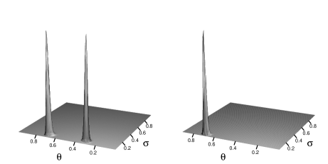
Figure 2: The likelihood function $L(\sigma,\theta)=p(\boldsymbol{R};\sigma,\theta)$ for the Perlin data with two unknown contributors (left). To the right the likelihood function after specifying the DNA profiles for two contributors.

The maximum likelihood estimates for $\sigma$ and $\theta$ are displayed in Table 3. The estimates $\hat{\sigma}$ and $\hat{\theta}$ are close to being independent with asymptotic correlations in the three situations for the Perlin data being -0.195, -0.042, and -0.042. For the Evett data it is -0.160 in both situations. For both data sets the estimated mixture proportions $\theta$ are remarkably close to the proportions used for constructing the DNA mixture. In contrast to the model using a uniformly distributed $\theta$, the Perlin data does not quite support the use of $\sigma=0.1$ although it is not far off.

For the Perlin data, if we include genotypes of the minor contributor as a potential contributor we get better estimates of the parameters which is reflected in the narrower confidence intervals. When further including the DNA profiles of both contributors as known, the estimates do not change at all. For the Evett dataset, specifying genetic information on a potential contributor barely changes the estimates.

For the Perlin data — where $\sigma\approx 0.07$ — a 95% prediction interval for the heterozygote balance $Hb$ is $0.759\leq Hb\leq 1.318$. For the Evett case the generic peak imbalance is a bit higher, resulting in a slightly wider range of expected heterozygote balance, $0.687\leq Hb\leq 1.456$. Note that for both the Perlin and the Evett data the model leads to heterozygote balances that comply with the recommendation in Bill et al. (2005).

Table 3: Joint maximum likelihood estimates of the mixture ratio and peak imbalance. The estimates of $\theta$ reflect the ratios used for constructing the data; a 7:3 ratio for the Perlin data, and a 10:1 ratio for the Evett data.

Perlin data
Genotype information	$\hat{\sigma}$	99% CI	$\hat{\theta}$	99% CI
Both contributors unknown	0.070	(0.040, 0.100)	0.692	(0.658, 0.727)
One known potential contributor	0.067	(0.041, 0.094)	0.696	(0.666, 0.725)
Both contributors known	0.067	(0.041, 0.094)	0.696	(0.667, 0.725)
Evett data
Genotype information	$\hat{\sigma}$	99% CI	$\hat{\theta}$	99% CI
Both contributors unknown	0.096	(0.044, 0.147)	0.895	(0.858, 0.932)
One known potential contributor	0.096	(0.044, 0.147)	0.895	(0.858, 0.932)

3.3 Including prior information about $\sigma$ and $\theta$

In Section 3.1 it was seen that the DNA mixture can be modelled conditionally on the observed relative peak sizes for a fixed $\sigma$ and a uniform distribution for $\theta$. We now explain how to combine this model with prior information about the variability on $\sigma$ to perform Bayesian inference in the model.

It is possible to simulate from $p(\boldsymbol{c}_{1},\boldsymbol{c}_{2},\sigma,\theta\,|\,H,\boldsymbol{R})$, for example by using a Gibbs sampler which alternates between

1. sampling a pair $(\boldsymbol{c}_{1},\boldsymbol{c}_{2},\theta)$ of complete configurations of genotypes and mixture proportion given the current value of $\sigma$ and observed relative peak sizes;

2. sampling $\sigma$ given the pair of DNA profiles sampled in the above step, the sampled mixture proportion, and the observed relative peak sizes.

The first step is performed by sampling from the Bayesian network model of the DNA mixture after including likelihood evidence using $\sigma$ and $\boldsymbol{R}$. For the second step, $\sigma$ can be sampled by standard methods for univariate sampling. In particular, provided that the prior distribution on $\beta=1/\sigma^{2}\!-\!1$ is log-concave (for instance true for a gamma distribution), the distribution of $\beta$ for a known composition of the DNA mixture is also log-concave, which means that we can use adaptive rejection sampling (Gilks and Wild, 1992) for this step.

4 Case analysis

We now illustrate the use of the different estimation methods for a case analysis. In the Bayesian analysis, the uncertainty about the parameters is represented by their posterior distribution. For a full specification of the Bayesian model we have used a uniform prior distribution for $\theta$ and a Gamma distribution for $\beta=1/\sigma^{2}\!-\!1$ with parameters $\Gamma(3.6,49)$ throughout. The chosen prior distribution for $\beta$ corresponds to a 95% prior credibility interval of $(0.05,0.15)$ for $\sigma$, representing typical values for the variability of relative peak areas. In a specific application it would be appropriate to use a prior distribution reflecting the typical values obtained in a given forensic laboratory. Generally it is difficult to identify an informed prior for $\theta$, as this would depend strongly on the type of trace analysed, so the uniform prior seems most appropriate.

Although the Bayesian method does not involve estimation of parameters but rather integrates over these, it is interesting to compare posterior means and credibility intervals to corresponding quantities when using maximum likelihood. These are displayed for illustration in Table 4 for the case of one known potential contributor only.

Table 4: Bayesian estimates (posterior means) of the mixture ratio and peak imbalance with estimated 99% credibility intervals for the case of one known potential contributor.

	$\bar{\sigma}$	99% CrI	$\bar{\theta}$	99% CI
Perlin data	0.073	(0.052, 0.106)	0.695	(0.67, 0.73)
Evett data	0.095	(0.063, 0.152)	0.894	(0.86, 0.93)

The Bayesian estimates and intervals are similar to those in Table 3, but the estimate and credibility interval for the peak imbalance is shifted slightly to the right by the prior information. Also the posterior correlations between $\sigma$ and $\theta$ are similar to those obtained from the information matrix, $-0.034$ for the Perlin data and $-0.166$ for the Evett data.

4.1 Evidence calculation

4.1.1 Evett data

For the Evett data we use the known major contributor as a potential suspect and compare the hypotheses as in (3). Using the fitted parameters from Table 3 we find

$$\log_{10}LR=\log_{10}\frac{p(\boldsymbol{R}\,|\,H_{p},\hat{\sigma},\hat{\theta})}{p(\boldsymbol{R}\,|\,H_{d},\hat{\sigma},\hat{\theta})}=8.53414.$$

We have here used the MLE for the situation where the known profile is specified to be a potential contributor. Alternatively one could use a different MLE in numerator and denominator, corresponding to the different hypotheses considered.

As the likelihood ratio is calculated using the parameter estimates, we can assess the uncertainty of the estimate of $\log_{10}LR$ by parametric bootstrap: using the fitted parameters and the fact that relative sizes are Dirichlet distributed, we simulate 2000 new sets of relative peak sizes and estimate the parameters for each of these. A 99% bootstrap confidence interval for the $\log_{10}LR$ is then (8.53397, 8.53414). Note that this is very narrow, indicating that $\log_{10}LR$ is very accurately determined despite the uncertainty in $\sigma$ and $\theta$. Histograms of the bootstrap samples of parameter estimates and $\log_{10}LR$-values are displayed in Figure 3.

Figure 3: Bootstrap simulations of $\hat{\sigma}$, $\hat{\theta}$ and $\log_{10}LR$ for the Evett data, based on 2000 samples. The dashed lines indicate the values as estimated on the Evett data set.

The shape of the histograms indicate that the distribution of the estimates are well approximated by a Gaussian distribution. Note the very concentrated histogram for $\log_{10}LR$.

For the Bayesian analysis, the quantity of interest is the ratio of marginal likelihoods

$$LR=\frac{p(\boldsymbol{R}\,|\,H_{p})}{p(\boldsymbol{R}\,|\,H_{d})}$$

with both $\theta$ and $\sigma$ integrated out; the numerator and denominator can be estimated from the Monte Carlo samples as

$$p(\boldsymbol{R}\,|\,H_{p})\approx\frac{1}{N}\sum_{i=1}^{N}p(\boldsymbol{R}\,|\,H_{p},\sigma_{i})$$

and similarly for $p(\boldsymbol{R}\,|\,H_{d})$. This yields a $\log_{10}LR$ of 8.233, somewhat smaller than the value obtained by using maximum likelihood, but still representing extremely strong evidence that the suspect has contributed to the mixture.

The marginal likelihood ratio in the Bayesian setup does not have a variation but we can compare the posterior distribution of the parameters with the bootstrap distribution of their estimates in Figure 3. These are shown in Figure 4. Apart from the discretization of $\theta$ in the Bayesian model, they again identify about the same region of plausible values for the parameters.

Figure 4: Samples from the posterior distributions of $\sigma$ and $\theta$ for the Evett data. The dashed lines indicate the posterior mean.

4.1.2 Perlin data

For the Perlin data, we use the known minor contributor as a potential contributor, and consider the likelihood ratio for $H_{p}$ against $H_{d}$ resulting in $\log_{10}LR=14.942$ using the joint maximum likelihood estimate $(\hat{\theta},\hat{\sigma})$ with a 99% bootstrap confidence interval of (13.328, 15.075), i.e. a considerably wider interval than for the Evett data. The Monte Carlo estimate for $\log_{10}LR$ of the marginal likelihood ratio is 14.511. We have displayed histograms for bootstrapped parameter estimates and log-likelihood ratios in Figure 5 and histograms for the posterior distribution in Figure 6.

Figure 5: Bootstrap simulations of $\hat{\sigma}$, $\hat{\theta}$ and corresponding $\log_{10}LR(\sigma,\theta)$ for the Perlin data. The dashed lines indicate the values estimated from the Perlin data using the minor contributor as a potential contributor.

Figure 6: Samples from the posterior distributions of $\sigma$ and $\theta$ for the Perlin data. The dashed lines indicate the posterior mean.

Again, the histograms indicate that the sampling distributions of the estimates and posterior distributions are similar and reasonably approximated by a Gaussian distribution. Here the sampling distribution of $\log_{10}LR$ is more variable, indicating higher sensitivity to parameter uncertainty than for the Evett data. Still, all values of $\log_{10}LR$ in the confidence interval provide evidence that the potential contributor indeed did contribute to the mixture.

4.2 Mixture deconvolution

We produce a ranked list of probable profile pairs using the following trick, exploiting the fact that sampling a set of DNA profiles for the contributors is straightforward regardless of the choice of estimation method. We sample profile pairs $(\boldsymbol{c}_{1},\boldsymbol{c}_{2})$ from a DNA mixture model using the observed relative peak sizes and the estimation method of preference. For each of the sampled profile pairs we then calculate the probability of that particular pair, $p\{(\boldsymbol{c}_{1},\boldsymbol{c}_{2})\,|\,\boldsymbol{R}\}$. Adding up these probabilities for all the sampled profile pairs we get that they account for some total $p$ of the probability mass, implying that no undiscovered pair of profiles can have probability larger than $1-p$. Thus, if $k$ of the sampled profile-pairs all have probability larger than $1-p$ they must constitute the $k$ most probable profiles. Note that the number $k$ of most probable profiles is not fixed in advance, and that increasing the number of samples will result in a longer list of profiles. We illustrate this method using the Perlin data.

If the model is fitted using maximum likelihood estimates for $\sigma$ and $\theta$, we can sample possible profiles for the two contributors using the Bayesian network and thereby obtain pairs of profiles of high probability. The sampling revealed 13 different profiles with a total probability of $p=0.9992$. There were eight of these profiles with a probability larger than $1-p=0.0008$, implying that the $k=8$ most probable DNA profile pairs had been determined. For seven of the markers the genotypes were correctly identified; for the marker TH01 there is slight uncertainty whether the minor contributor supplied the allele 7 or 9; similarly, for markers D19 and VWA there is slight uncertainty about the allocation of alleles to the contributors. Table 5 displays the eight possible choices for the remaining three markers.

Table 5: The eight most probable contributor genotypes of the three uncertain markers for the Perlin data using the MLE for $\sigma$ and $\theta$. Correctly predicted genotypes are marked in bold.

	Major contributor			Minor contributor
rank	D19	TH01	VWA	D19	TH01	VWA	Prob.
1	12.2 15	7 9	17 17	14 14	6 7	18 18	0.647
2	12.2 15	7 9	17 18	14 14	6 7	17 17	0.261
3	12.2 14	7 9	17 17	15 15	6 7	18 18	0.054
4	12.2 14	7 9	17 18	15 15	6 7	17 17	0.022
5	14 15	7 9	17 17	12.2 12.2	6 7	18 18	0.006
6	12.2 15	7 9	17 17	14 14	6 9	18 18	0.004
7	14 15	7 9	17 18	12.2 12.2	6 7	17 17	0.002
8	12.2 15	7 9	17 18	14 14	6 9	17 17	0.001
Total probability							0.997

We note that for the Perlin data the most probable profile pair is the true one and the second most probable pair has a misclassification on only one marker, VWA. As for the analysis of evidential value, it is possible to assess the uncertainty of these rankings and the sensitivity to the choice of parameters, e.g. by bootstrap. We shall omit such further analysis here.

For the Bayesian analysis we use the Gibbs sampler to locate high probability pairs of profiles. In this case we obtain 27 different profiles for each contributor. Subsequently we again use the Gibbs sampler to obtain the posterior probability $p\{(\boldsymbol{c}_{1},\boldsymbol{c}_{2})\,|\,\boldsymbol{R}\}$ for each pair as

$$p\{(\boldsymbol{c}_{1},\boldsymbol{c}_{2})\,|\,\boldsymbol{R}\}\approx\frac{1}{N}\sum_{i=1}^{N}p\{(\boldsymbol{c}_{1},\boldsymbol{c}_{2})\,|\,\boldsymbol{R},\sigma_{i}\}.$$

This yields a total probability $p=0.998$ for the 27 profiles and identifies nine profiles with a probability larger than the resulting threshold $1-p=0.002$. Also in the Bayesian analysis all genotypes were correctly identified for seven of the markers. The genotypes of the profile pairs for the remaining three markers are displayed in Table 6.

Table 6: The nine most probable contributor genotypes of the three uncertain markers for the Perlin data in a Bayesian analysis.

	Major contributor			Minor contributor
rank	D19	TH01	VWA	D19	TH01	VWA	Prob.
1	12.2 15	7 9	17 17	14 14	6 7	18 18	0.548
2	12.2 15	7 9	17 18	14 14	6 7	17 17	0.300
3	12.2 14	7 9	17 18	15 15	6 7	17 17	0.061
4	12.2 14	7 9	17 17	15 15	6 7	18 18	0.055
5	12.2 15	7 9	17 17	14 14	6 9	18 18	0.007
6	12.2 15	7 9	17 18	14 14	6 9	17 17	0.005
7	12.2 15	7 9	17 17	14 14	6 7	17 18	0.005
8	14 15	7 9	17 17	12.2 12.2	6 7	18 18	0.005
9	14 15	7 9	17 18	12.2 12.2	6 7	17 17	0.003
Total probability							0.988

The Bayesian analysis reveals the same two profile pairs as the most probable but slightly reverses the ranking of profile pairs with smaller probabilities. Note, though, that the probabilities in Table 6 are Monte Carlo estimates with a standard error up to 3% and thus the mutual ranking of profiles with very similar probabilities is uncertain. In other words, the four most highly ranked configurations are definitely the top four on the list, whereas the mutual ranking of number three and four could be reversed, although this is unlikely. Similarly, the correct mutual ranking of the last five could easily be reversed in comparison with the ranking in the table.

5 Discussion

In the present article we have demonstrated how both the mixture proportions and the unknown variance factor in the model used by Cowell et al. (2007a) can be estimated and its uncertainty incorporated into further analysis of the DNA trace. The analysis shows that there is sufficient information in a single trace to do so using only the peak sizes for the data at hand, if the variance factor $\sigma$ is taken to be marker independent.

We have illustrated how it is possible to assess the performance of a particular method for a given case. It would be well worthwhile to carry out a further study on the general performance, for example of the stability of the method for mixture deconvolution. However, we would like to emphasise that by performing a bootstrap analysis we get an indication of the information that data from mixtures of similar composition would provide about the questions in mind and the bootstrap analyses do indicate a considerable stability of the findings.

There might be good reasons to believe that the peak imbalance $\sigma$ differs across markers. As there is limited information in the data from a single case we have for practical reasons chosen to ignore this variation and use a single $\sigma$ for each case. An alternative way of accommodating marker dependence on the generic variability would be to assume that the parameter $\beta=1/\sigma^{2}\!-\!1$ in the gamma model (1) depends on $m$ as $\beta_{m}=\lambda\delta_{m}$ where $\lambda$ depends only on the case at hand and $\delta_{m}$ is marker dependent but independent of the case considered. One could then use laboratory data to estimate $\delta_{m}$ and only adapt $\lambda$ to the case. This methodology would only demand minor technical variations for the Bayesian and maximum likelihood methods developed in this paper. Generally, prior information on the total amount of DNA would also be available which could be used to improve the Bayesian analysis by using an informed prior distribution for $\lambda$.

We have only considered the simplest model with a fixed number of contributors and no artefacts in the form of stutter, dropout, etc. Maximum likelihood estimates for the parameters can still be found extending to the case of multiple contributors, but as there would be more mixture proportions to estimate, larger confidence intervals for the parameter estimates are to be expected. Extensions (Cowell et al., 2011, 2013) involve even more parameters which need to be estimated in a similar way and it certainly adds to the general complexity of the problem, as does issues of gene frequency uncertainties etc. (Green and Mortera, 2009). We expect to address these issues in the future.

References

- Bill et al. (2005) Bill, M., Gill, P., Curran, J., Clayton, T., Pinchin, R., Healy, M., Buckleton, J., 2005. PENDULUM – a guideline-based approach to the interpretation of STR mixtures. Forensic Science International 148, 181–189.
- Butler (2005) Butler, J. M., February 2005. Forensic DNA Typing: Biology, Technology, and Genetics of STR Markers, 2nd Edition. Elsevier ACADEMIC PRESS.
- Butler et al. (2003) Butler, J. M., Schoske, R., Vallone, P. M., Redman, J. W., Kline, M. C., 2003. Allele frequencies for 15 autosomal loci on U.S. Caucasian, African American, and Hispanic populations. Journal of Forensic Science 48 (4).
- Clayton et al. (1998) Clayton, T., Whitaker, J., Sparkes, R., Gill, P., 1998. Analysis and interpretation of mixed forensic stains using DNA STR profiling. Forensic Science International 91 (1), 55–70.
- Cowell (2009) Cowell, R. G., 2009. Validation of an STR peak area model. Forensic Science International: Genetics 3 (3), 193–199.
- Cowell et al. (2013) Cowell, R. G., Graversen, T., Lauritzen, S., Mortera, J., 2013. Analysis of DNA mixtures with artefacts, arXiv:1302:4404.
- Cowell et al. (2007a) Cowell, R. G., Lauritzen, S. L., Mortera, J., January 2007a. A gamma model for DNA mixture analyses. Bayesian Analysis 2 (2), 333–348.
- Cowell et al. (2007b) Cowell, R. G., Lauritzen, S. L., Mortera, J., 2007b. Identification and separation of DNA mixtures using peak area information. Forensic Science International 166, 28–34.
- Cowell et al. (2011) Cowell, R. G., Lauritzen, S. L., Mortera, J., 2011. Probabilistic expert systems for handling artifacts in complex DNA mixtures. Forensic Science International: Genetics 5, 202–209.
- Curran (2008) Curran, J. M., 2008. A MCMC method for resolving two person mixtures. Science and Justice 48, 168–177.
- Evett et al. (1998) Evett, I., Gill, P., Lambert, J., 1998. Taking account of peak areas when interpreting mixed DNA profiles. Journal of Forensic Science 43 (1), 62–69.
- Gilks et al. (1996) Gilks, W. R., Richardson, S., Spiegelhalter, D. J., 1996. Markov Chain Monte Carlo Methods in Practice. Chapman and Hall, New York.
- Gilks and Wild (1992) Gilks, W. R., Wild, P., 1992. Adaptive rejection sampling for Gibbs sampling. Applied Statistics 41 (2), 337–348.
- Gill et al. (2006) Gill, P., Brenner, C., Buckleton, J., Carracedo, A., Krawczak, M., Mayr, W., Morling, N., Prinz, M., Schneider, P., Weir, B., 2006. DNA commission of the international society of forensic genetics: Recommendations on the interpretation of mixtures. Forensic Science International 160 (2), 90 – 101.
- Gill et al. (2008) Gill, P., Curran, J., Neumann, C., Kirkham, A., Clayton, T., Whitaker, J., Lambert, J., 2008. Interpretation of complex DNA profiles using empirical models and a method to measure their robustness. Forensic Science International: Genetics 2 (2), 91–103.
- Green and Mortera (2009) Green, P. J., Mortera, J., 2009. Sensitivity of inferences in forensic genetics to assumptions about founder genes. Annals of Applied Statistics 3 (2), 731–763.
- HUGIN API (2009) HUGIN API, 2009. HUGIN API Reference Manual. Hugin Expert A/S.
- Konis and Hugin Expert A/S (2010) Konis, K., Hugin Expert A/S, 2010. RHugin. R package version 7.3-1.
- Perlin and Szabady (2001) Perlin, M., Szabady, B., 2001. Linear mixture analysis: a mathematical approach to resolving mixed DNA samples. Journal of Forensic Science 46, 1372–1378.
- Perlin et al. (2011) Perlin, M. W., Legler, M. M., Spencer, C. E., Smith, J. L., Allan, W. P., Belrose, J. L., Duceman, B. W., 2011. Validating TrueAllele® DNA mixture interpretation. Journal of Forensic Sciences 56 (6), 1430–1447.
- Puch-Solis et al. (2012) Puch-Solis, R., Rodgers, L., Mazumder, A., Pope, S., Evett, I., Curran, J., Balding, D., 2012. Evaluating forensic DNA profiles using peak heights, allowing for multiple donors, allelic dropout and stutters. Tech. rep., LGC Research Report LGC/P/2012/138.
- R Development Core Team (2011) R Development Core Team, 2011. R: A Language and Environment for Statistical Computing. R Foundation for Statistical Computing, Vienna, Austria, ISBN 3-900051-07-0.
- Wang et al. (2006) Wang, T., Xue, N., Birdwell, J. D., 2006. Least-square deconvolution: A framework for interpreting short tandem repeat mixtures. Journal of Forensic Sciences 51 (6), 1284–1297.