Generalized acceleration theorem for spatiotemporal Bloch waves

Abstract

A representation is put forward for wave functions of quantum particles in periodic lattice potentials subjected to homogeneous time-periodic forcing, based on an expansion with respect to Bloch-like states which embody both the spatial and the temporal periodicity. It is shown that there exists a generalization of Bloch’s famous acceleration theorem which grows out of this representation, and captures the effect of a weak probe force applied in addition to a strong dressing force. Taken together, these elements point at a “dressing and probing” strategy for coherent wave-packet manipulation, which could be implemented in present experiments with optical lattices.

I Introduction

The so-called acceleration theorem for wave-packet motion in periodic potentials, formulated already in 1928 by Bloch, Bloch28 has proven to be of outstanding value to solid-state physics for understanding the dynamics of Bloch electrons within a semiclassical picture. AshcroftMermin76 ; Kittel87 In its most-often used variant, this theorem states that if we consider an electronic wave packet in a spatially periodic lattice, which is centered in $k$ space around some wave vector $\vec{k}_{\rm c}$, and if an external electric field $\vec{E}(t)$ is applied under single-band conditions, then this center wave vector evolves in time according to $\hbar\dot{\vec{k}}_{\rm c}(t)=-e\vec{E}(t)$, with $-e$ being the electronic charge. Perhaps its best-known application is the explanation of Bloch oscillations of particles exposed to a homogeneous, constant force, RoskosEtAl92 ; FeldmannEtAl92 ; Feldmann92 ; WaschkeEtAl93 ; IgnatovEtAl94 ; RotvigEtAl95 ; IgnatovEtAl95 ; BouchardLuban95 ; UnterrainerEtAl96 ; LyssenkoEtAl97 ; LenzEtAl99 ; BenDahanEtAl96 ; MorschEtAl01 which we recapitulate here in the simplest guise: Take a particle in a one-dimensional tight-binding energy band $E(k)=-(W/2)\cos(ka)$, where $W$ is the band width and $a$ denotes the lattice period. Assume that the particle’s wave packet is centered around $k_{\rm c}(0)$ initially and subjected to a homogeneous force of strength $F$. Then the acceleration theorem, now taking the form

$$\hbar\dot{k}_{\rm c}(t)=F\;,$$ (1)

tells us $k_{\rm c}(t)=k_{\rm c}(0)+Ft/\hbar$, so that the packet moves through $k$ space at a constant rate. Bloch28 According to another classic work by Jones and Zener, JonesZener34 the particle’s group velocity $v_{\rm g}(t)$ in real space is determined, quite generally, by the derivative of $E(k)$ with respect to $k$ when evaluated at the moving center $k_{\rm c}(t)$,

$$v_{\rm g}(t)=\frac{1}{\hbar}\left.\frac{{\rm d}E}{{\rm d}k}\right|_{k_{\rm c}(t)}\;.$$ (2)

In our case, this relation immediately gives

$$v_{\rm g}(t)=\frac{Wa}{2\hbar}\sin\!\big{(}k_{\rm c}(0)a+\omega_{\rm B}t\big{)}\;,$$ (3)

implying that the particle’s response to the constant force is an oscillating motion with the Bloch frequency Zener34 $\omega_{\rm B}=Fa/\hbar$. This elementary example, to which we will come back later in Sec. IV, strikingly illustrates the power of this type of approach. But an obvious restriction stems from the necessity to remain within the scope of the single-band approximation; the above acceleration theorem (1) is put out of action when several Bloch bands are substantially coupled by the external force. Nonetheless, in the present work we demonstrate that there exists a generalization of the acceleration theorem which can be applied even under conditions of strong interband transitions. Specifically, we consider situations in which a Bloch particle is subjected to a strong oscillating force which possibly induces pronounced transitions between the unperturbed energy bands. By abandoning the customary crystal-momentum representation Callaway74 and introducing an alternative Floquet representation instead, we show that the effect of an additional force then is well captured by another acceleration theorem which closely mimics the spirit of the original. We obtain two major results: The Floquet analog (32) of Bloch’s acceleration theorem (1), and the Floquet analog (42) of the Jones-Zener expression (2) for the group velocity. These findings are particularly useful for control applications, when a strong oscillating field “dresses” the lattice and thus significantly alters its band structure, while a second, comparatively weak homogeneous force is employed to effectuate controlled population transfer. We first outline the formal mathematical arguments in Secs. II and III, and then we give two applications of topical interest, discussing “super” Bloch oscillations in Sec. IV and coherently controlled interband population transfer in Sec. V. Although we restrict ourselves here for notational simplicity to one-dimensional lattices, our results can be carried over to general, higher-dimensional settings.

II The Floquet representation

We consider a particle of mass $m$ moving in a one-dimensional lattice potential $V(x)=V(x+a)$ with spatial period $a$ under the influence of a homogeneous, time-dependent force $F(t)$, as described by the Hamiltonian

$$\widetilde{H}_{0}(x,t)=\frac{p^{2}}{2m}+V(x)-F(t)x\;.$$ (4)

Subjecting the particle’s wave function $\widetilde{\psi}(x,t)$ to the unitary transformation

$$\widetilde{\psi}(x,t)=\exp\!\left(\frac{{\rm i}}{\hbar}x\!\int_{0}^{t}\!{\rm d}\tau\,F(\tau)\right)\psi(x,t)\;,$$ (5)

the new function $\psi(x,t)$ obeys the Schrödinger equation

$${\rm i}\hbar\frac{\partial}{\partial t}\psi(x,t)=H_{0}(x,t)\psi(x,t)\;,$$ (6)

with the transformed Hamiltonian

$$H_{0}(x,t)=\frac{1}{2m}\left(p+\int_{0}^{t}\!{\rm d}\tau\,F(\tau)\right)^{2}+V(x)\;.$$ (7)

Now let us further assume that the force $F(t)$ is periodic in time with period $T$, such that its one-cycle integral either vanishes or equals an integer multiple of $\hbar$ times the reciprocal lattice wave number $2\pi/a$:

$$\int_{0}^{T}\!{\rm d}t\,F(t)=r\times\hbar\frac{2\pi}{a}\quad,\quad r=0,\pm 1,\pm 2,\ldots\;.$$ (8)

For example, this is accomplished by a monochromatic oscillating force with an additional static bias,

$$F(t)=F_{r}+F_{\rm ac}\cos(\omega t)\;,$$ (9)

provided the latter satisfies the condition $F_{r}a=r\hbar\omega$. Then the Floquet theorem guarantees that the time-dependent Schrödinger equation (6) admits a complete set of spatiotemporal Bloch waves, Holthaus92 ; DreseHolthaus97 ; ArlinghausHolthaus10 that is, of solutions of the form

$$\psi_{n,k}(x,t)=\exp\!\big{(}{\rm i}kx-{\rm i}\varepsilon_{n}(k)t/\hbar\big{)}u_{n,k}(x,t)\;,$$ (10)

with spatially and temporally periodic functions

$$u_{n,k}(x,t)=u_{n,k}(x+a,t)=u_{n,k}(x,t+T)\;.$$ (11)

As usual, $n$ is the band index and $k$ a wave number; $\varepsilon_{n}(k)$ thus is the quasienergy dispersion relation for the $n$th band. If $r=0$ in Eq. (8), the existence of these solutions is obvious, because then $H_{0}(x,t)=H_{0}(x+a,t)=H_{0}(x,t+T)$, so that the wave functions (10) generalize the customary Bloch waves Bloch28 for particles in spatially periodic lattice potentials by also accounting for the temporal periodicity of the driving force. When $r\neq 0$, so that $H_{0}(x,t)$ itself is not periodic in time, spatiotemporal Bloch waves (10) emerge nonetheless because $k$ is projected to the first quasimomentum Brillouin zone, as first discussed by Zak. Zak93 In any case, the quasienergies $\varepsilon_{n}(k)$ may depend in a complicated manner on the parameters of the driving force, and the wave functions $\psi_{n,k}(x,t)$ pertaining to a single quasienergy band may be nontrivial mixtures of several unperturbed energy bands. For later use, we observe that their spatial parts

$$\varphi_{n,k}(x,t)=\exp({\rm i}kx)u_{n,k}(x,t)$$ (12)

obey the quasienergy eigenvalue equation

$$\left(H_{0}(x,t)-{\rm i}\hbar\frac{\partial}{\partial t}\right)\varphi_{n,k}(x,t)=\varepsilon_{n}(k)\varphi_{n,k}(x,t)\;,$$ (13)

as follows immediately when plugging the solutions (10) into the Schrödinger equation (6). Throughout, we adopt the standard normalization

$$\int_{-\infty}^{\infty}\!{\rm d}x\,\varphi^{*}_{n^{\prime},k^{\prime}}(x,t)\varphi_{n,k}(x,t)=\frac{2\pi}{a}\delta_{n,n^{\prime}}\delta(k-k^{\prime})\;.$$ (14)

An arbitrary wave packet $\psi(x,t)$ may now be expanded with respect to these spatiotemporal Bloch waves, and written in the form

$$\psi(x,t)=\sum_{n}\sqrt{\frac{a}{2\pi}}\int_{\cal B}\!{\rm d}k\,g_{n}(k,t)\varphi_{n,k}(x,t)\;,$$ (15)

with ${\cal B}=[-\pi/a,\pi/a[$ denoting the fundamental Brillouin zone. The expansion coefficients $g_{n}(k,t)$ depend on the way the system has been prepared and on the way the driving force has been turned on, whereas the basis functions $\varphi_{n,k}(x,t)$ and their quasienergies $\varepsilon_{n}(k)$ are given by the eigenvalue equation (13) and obviously are independent of such details. Clearly, one has

$$g_{n}(k,t)=g_{n}(k,0)\exp\!\big{(}-{\rm i}\varepsilon_{n}(k)t/\hbar\big{)}\;,$$ (16)

so that the populations $|g_{n}(k,t)|^{2}$ remain constant in time. This expansion (15), referred to as the Floquet representation of the wave packet, is formally reminiscent of its customary crystal-momentum representation, that is, of an expansion with respect to the Bloch states of the unperturbed potential $V(x)$ which underlies the standard acceleration theorem. Callaway74 ; GrecchiSacchetti01 There are, however, substantial differences which become most clear when considering a wave packet occupying a single quasienergy band,

$$\psi(x,t)=\sqrt{\frac{a}{2\pi}}\int_{\cal B}\!{\rm d}k\,g(k,t)\varphi_{k}(x,t)\;;$$ (17)

here and in the following, we omit the band index $n$ for ease of notation. Now this wave packet (17) may describe, for instance, the dynamics in a situation where two unperturbed energy bands are resonantly coupled by the driving force $F(t)$; consequently, in a crystal-momentum representation one would have to account for Rabi-type oscillations between these two bands by coefficients which quantify the oscillating band populations. In the Floquet respresentation, on the other hand, the Rabi oscillations are already incorporated into the basis states (10), so that one merely encounters single quasienergy band dynamics, with the remaining time evolution of $g(k,t)$ simply given by Eq. (16). Thus, although the external force effectuates transitions between the unperturbed Bloch bands, there are no inter-quasienergy band transitions; $|g(k,t)|^{2}$ remains constant in time. Second, even in a situation where $F(t)$ does not couple different energy bands, the wave packet’s center $k_{\rm c}(t)$ evolves according to the standard acceleration theorem $\hbar\dot{k}_{\rm c}=F$ in the crystal-momentum representation, whereas in the Floquet representation the moment

$$\langle k\rangle=\int_{\cal B}\!{\rm d}k\,k|g(k,t)|^{2}$$ (18)

obviously stays constant in time. In short, an expansion of the wave packet with respect to the spatiotemporal Bloch waves (10) implies constant coefficients, and hence constant occupation probabilities, if the external force $F(t)$ adheres to the specification (8). This formal shift of the dynamics from the occupation numbers to the basis states which is implied by the Floquet representation now allows for a clear and physically transparent description of the additional effects which emerge when the external force does not obey Eq. (8); these effects are captured by the generalized acceleration theorem exposed in the following.

III The Floquet acceleration theorem

We take a wave packet occupying a single quasienergy band and stipulate that in addition to the possibly strong driving force $F(t)$ there is a second homogeneous force $F_{\rm p}(t)$ which we denote as the probe force; this is assumed to be sufficiently weak so that it does not introduce transitions among different quasienergy bands. To be precise, the total Hamiltonian now reads

$$\widetilde{H}(x,t)=\frac{p^{2}}{2m}+V(x)-F(t)x-F_{\rm p}(t)x\;,$$ (19)

where the time-periodic force $F(t)$ is resonant in the sense of Eq. (8) and thus creates a basis of spatiotemporal Bloch waves (10), whereas the probe force $F_{\rm p}(t)$ also is spatially homogeneous, but not necessarily periodic in time. After performing the unitary transformation (5), we obtain the Hamiltonian in the form

$$H(x,t)=H_{0}(x,t)-F_{\rm p}(t)x\;,$$ (20)

with $H_{0}(x,t)$ given by Eq. (7). Moreover, we start from an initial wave packet of the form (17). Because of the additional probe force $F_{\rm p}(t)$, the time evolution of $g(k,t)$ is no longer given by Eq. (16); the aim now is to find an effective Hamiltonian ${\cal H}$ which governs the resulting dynamics of $g(k,t)$, under the proposition that this remains restricted to the single, initially occupied quasienergy band.

Exploiting the normalization (14), we have

$$g(k,t)=\sqrt{\frac{a}{2\pi}}\int\!{\rm d}x\,\varphi_{k}^{*}(x,t)\psi(x,t)\;.$$ (21)

This gives

$${\rm i}\hbar\frac{\partial g}{\partial t} = \sqrt{\frac{a}{2\pi}}\int\!{\rm d}x\left({\rm i}\hbar\frac{\partial\varphi_{k}^{*}}{\partial t}\psi+\varphi_{k}^{*}H\psi\right)$$ (22)

$$= \sqrt{\frac{a}{2\pi}}\int\!{\rm d}x\left(\left[H_{0}-{\rm i}\hbar\frac{\partial}{\partial t}\right]\varphi_{k}\right)^{*}\psi$$

$$-\sqrt{\frac{a}{2\pi}}F_{\rm p}\int\!{\rm d}x\,\varphi_{k}^{*}x\psi\;,$$

having suppressed the arguments $x$ and $t$ for better legibility; all integrals here are taken over the entire lattice. In the first term on the right-hand side of this equation we exploit the quasienergy eigenvalue equation, Eq. (13), yielding $\varepsilon(k)g(k,t)$. For rewriting the second term we use

$$\varphi_{k}^{*}x={\rm i}\partial_{k}\varphi_{k}^{*}-{\rm i}{\rm e}^{-{\rm i}kx}\partial_{k}u_{k}^{*}\;,$$ (23)

which is obtained by taking the derivative of the complex conjugate to Eq. (12) with respect to $k$, and leads to

$$\sqrt{\frac{a}{2\pi}}\int\!{\rm d}x\,\varphi_{k}^{*}x\psi = {\rm i}\partial_{k}g-{\rm i}\sqrt{\frac{a}{2\pi}}\int\!{\rm d}x\,{\rm e}^{-{\rm i}kx}\partial_{k}u_{k}^{*}\psi$$ (24)

$$= {\rm i}\partial_{k}g-{\rm i}\langle\partial_{k}u_{k}|u_{k}\rangle g\;.$$

For making the final step, we have resubstituted the expression (17) for $\psi$ and have made use of the identity

$$\int\!{\rm d}x\,{\rm e}^{{\rm i}(k^{\prime}-k)x}u_{k^{\prime}}\partial_{k}u_{k}^{*}=\frac{2\pi}{a}\delta(k-k^{\prime})\langle\partial_{k}u_{k}|u_{k}\rangle\;,$$ (25)

with the scalar product

$$\langle\partial_{k}u_{k}|u_{k}\rangle=\int_{0}^{a}\!{\rm d}x\,u_{k}(x,t)\partial_{k}u_{k}^{*}(x,t)$$ (26)

being given by an integral over a single lattice period. Note that

$$\langle u_{k}|u_{k}\rangle=1\;,$$ (27)

as an immediate consequence of Eq. (14), which implies

$$\langle\partial_{k}u_{k}|u_{k}\rangle+\langle\partial_{k}u_{k}|u_{k}\rangle^{*}=0\;,$$ (28)

so that $\langle\partial_{k}u_{k}|u_{k}\rangle$ is purely imaginary. Collecting all the pieces, we obtain the desired evolution equation

$${\rm i}\hbar\frac{\partial}{\partial t}g(k,t)={\cal H}g(k,t)\;,$$ (29)

with the effective Hamiltonian for the Floquet representation,

$${\cal H}=\varepsilon(k)-{\rm i}F_{\rm p}\partial_{k}-F_{\rm p}\,{\rm Im}\langle\partial_{k}u_{k}|u_{k}\rangle\;.$$ (30)

From this expression we deduce the generalized acceleration theorem, that is, the acceleration theorem for the Floquet representation: Since the moment (18) obeys the the equation

$$\frac{{\rm d}}{{\rm d}t}\langle k\rangle=\frac{{\rm i}}{\hbar}\langle[{\cal H},k]\rangle$$ (31)

and the commutator appearing here on the right-hand side is easily evaluated, ${\rm i}[{\cal H},k]=F_{\rm p}$, we are directly led to

$$\hbar\frac{{\rm d}}{{\rm d}t}\langle k\rangle(t)=F_{\rm p}(t)\;.$$ (32)

This is the central result of the present work; its analogy to the standard acceleration theorem (1) for the crystal-momentum representation is evident. Observe that there is an intuitively clear reason for the appearance of the term proportional to $\langle\partial_{k}u_{k}|u_{k}\rangle$ in the effective Hamiltonian (30): The twofold periodic parts $u_{k}(x,t)$ of the spatiotemporal Bloch waves are obtained by solving the eigenvalue equation (13). This is done for each wave number $k$ separately, so that one is free to bestow upon each eigensolution an arbitrary phase factor $\exp({\rm i}\theta(k))$. On the other hand, the evolution equation (29) for the wave function $g(k,t)$ in the Floquet representation naturally establishes a “connection” between those different eigensolutions Simon83 ; Berry84 and therefore requires information about the gauge function $\theta(k)$; this is provided by the expression $\langle\partial_{k}u_{k}|u_{k}\rangle$. Note further that when multiplying Eq. (29) by $g^{*}(k,t)$ and subtracting the complex conjugate of the resulting equation, this piece drops out, and one is left with

$$\left(\frac{\partial}{\partial t}+\frac{F_{\rm p}(t)}{\hbar}\frac{\partial}{\partial k}\right)|g(k,t)|^{2}=0\;.$$ (33)

Thus, $|g(k,t)|^{2}$ does not depend on $k$ and $t$ separately, but rather on the combination $k-\int_{0}^{t}\!{\rm d}\tau\,F_{\rm p}(\tau)/\hbar$, so that the distribution $g(k,t)$ moves through the Floquet $k$ space without change of shape, again in precise analogy to the classic behavior. Bloch28 But we reemphasize that this seemingly simple dynamics might be unrecognizable in the usual crystal-momentum representation, because the system might undergo violent transitions between different energy bands when monitored in a basis of time-independent Bloch waves.

As the introductory example has shown, the standard (crystal-momentum) acceleration theorem develops its main power in combination with the Jones-Zener expression (2) for the wave packet’s group velocity in real space, and the question naturally arises whether there exists a similar connection in the Floquet representation. Obviously, one can establish a relation corresponding to Eq. (2) by applying a stationary-phase argument to the expansion (15), but here we follow an alternative line of reasoning which may be found particularly enlightening. Considering a well-localized wave packet $\widetilde{\psi}(x,t)$ in the original frame of reference to which the Hamiltonian operators (4) and (19) pertain, that packet’s group velocity is given by

$$v_{\rm g}(t) = \frac{{\rm d}}{{\rm d}t}\langle\widetilde{\psi}(x,t)|x|\widetilde{\psi}(x,t)\rangle$$ (34)

$$= \frac{1}{m}\langle\widetilde{\psi}(x,t)|p|\widetilde{\psi}(x,t)\rangle\;.$$

On the other hand, exploiting the operator identity

$${\rm e}^{-ikx}p{\rm e}^{ikx}=p+\hbar k\;,$$ (35)

the eigenvalue equation (13) transforms into the even more basic eigenvalue equation

$$\left(H_{k}(x,t)-{\rm i}\hbar\frac{\partial}{\partial t}\right)u_{n,k}(x,t)=\varepsilon_{n}(k)u_{n,k}(x,t)$$ (36)

for the periodic core pieces $u_{n,k}(x,t)$ of the spatiotemporal Bloch waves (10), invoking the parametrically $k$-dependent operator

$$H_{k}(x,t)=\frac{1}{2m}\left(p+\hbar k+\int_{0}^{t}\!{\rm d}\tau\,F(\tau)\right)^{2}+V(x)\;.$$ (37)

This eigenvalue problem can efficiently be implemented for numerical calculations. DreseHolthaus97 It also manifestly contains the origin of the condition (8) imposed on the oscillating force $F(t)$, since $k$ is reduced to fall within ${\cal B}$. Most importantly, this eigenvalue problem (36) poses itself in an extended Hilbert space made up of functions $u_{n,k}(x,t)$ which are periodic in both space and time, in accordance with Eq. (11). Consequently, “time” has to be regarded as a coordinate in this extended Hilbert space and therefore needs to be integrated over when forming a scalar product, just like any spatial coordinate. Thus, the natural scalar product in this extended Hilbert space is given by Sambe73

$$\langle\!\langle\,\cdot\,|\,\cdot\,\rangle\!\rangle\equiv\frac{1}{T}\int_{0}^{T}\!{\rm d}t\,\langle\,\cdot\,|\,\cdot\,\rangle\;,$$ (38)

with $\langle\,\cdot\,|\,\cdot\,\rangle$ denoting the standard scalar product in the original, physical Hilbert space, as already employed in Eqs. (26) and (27). It follows that the quasienergies $\varepsilon_{n}(k)$ can be written as diagonal elements of the matrix of the quasienergy operator,

$$\varepsilon_{n}(k)=\langle\!\langle u_{n,k}|H_{k}-{\rm i}\hbar\partial_{t}|u_{n,k}\rangle\!\rangle\;,$$ (39)

inviting us to make use of an analog of the Hellmann-Feynman theorem: Sambe73

$$\frac{{\rm d}}{{\rm d}k}\varepsilon_{n}(k) = \langle\!\langle u_{n,k}|\frac{{\rm d}H_{k}}{{\rm d}k}|u_{n,k}\rangle\!\rangle$$ (40)

$$= \frac{\hbar}{m}\langle\!\langle u_{n,k}|p+\hbar k+\int_{0}^{t}\!{\rm d}\tau\,F(\tau)|u_{n,k}\rangle\!\rangle$$

$$= \frac{\hbar}{m}\langle\!\langle\widetilde{\psi}_{n,k}|p|\widetilde{\psi}_{n,k}\rangle\!\rangle\;.$$

In the final step we have undone the shift (35); the wave functions $\widetilde{\psi}_{n,k}(x,t)$ then denote the functions which are obtained from the spatiotemporal Bloch waves (10) by inverting the transformation (5). Comparison of Eqs. (34) and (40), keeping in mind the definition (38), now yields the desired relation: Supposing that $\widetilde{\psi}(x,t)=\widetilde{\psi}_{n,k_{0}}(x,t)$ were made up from a single spatiotemporal Bloch wave labeled by $n$ and $k_{0}$, say, one would obtain the formal identity

$$\overline{v}_{\rm g}\equiv\frac{1}{T}\int_{0}^{T}\!{\rm d}t\,v_{\rm g}(t)=\frac{1}{\hbar}\left.\frac{{\rm d}\varepsilon_{n}}{{\rm d}k}\right|_{k_{0}}\;.$$ (41)

But this is not what we want, because an individual spatiotemporal Bloch wave is uniformly extended over the lattice and thus does not correspond to a “group” which propagates in space. Rather, we require a wave packet (17) which is reasonably well centered in the Floquet $k$ space, with a center $\langle k\rangle$ given by Eq. (18). Then we have

$$\overline{v}_{\rm g}=\frac{1}{\hbar}\left.\frac{{\rm d}\varepsilon_{n}}{{\rm d}k}\right|_{\langle k\rangle}$$ (42)

to good accuracy, so that the cycle-averaged group velocity of the Floquet wave packet is given by the derivative of its quasienergy dispersion relation, evaluated at its center $\langle k\rangle$. Again, this Floquet relation (42) closely mimics its historic crystal-momentum antecessor, given by Eq. (2). In contrast to the equation of motion (32) for $\langle k\rangle$ itself, which holds exactly within a single quasienergy band setting, this relation (42) is an approximation which holds the better, the narrower the packet’s Floquet $k$ space distribution. Although it seems self-evident, it might be worthwhile to stress that the argument required to evaluate the derivative (42) is Floquet $\langle k\rangle$, not crystal momentum $k_{\rm c}$.

IV Super Bloch oscillations

The phenomenon termed “super” Bloch oscillations HallerEtAl10 arises when a Bloch particle is subjected to both a static (dc) and an oscillating (ac) force, such that an integer multiple of the ac frequency is only slightly detuned from the Bloch frequency associated with the dc component of the force. HallerEtAl10 ; KolovskyKorsch10 ; AlbertiEtAl09 ; KudoMonteiro11 Although the effect itself appears almost trivial from the mathematical point of view, we nonetheless dwell on this at some length, because it provides a particularly instructive example for juxtaposing the familiar crystal-momentum representation to the Floquet representation introduced in Sec. II and for demonstrating in detail how they match. To be definite, we consider the total force to be of the form

$$F(t)=\Theta(t-t_{0})\left[F_{\rm dc}+F_{\rm ac}\cos(\omega t)\right]\;,$$ (43)

where $\Theta(t)$ denotes the Heaviside function, so that both the dc and the ac component of the force are turned on instantaneously and simultaneously at $t_{0}$; that moment $t_{0}$ thus determines the relative phase between the Bloch oscillations caused by the dc component and the driving oscillations of the ac component.

The basic assumptions now are that (i) we are given an initial wave packet which occupies a single energy band, being centered around $k_{\rm c}(t_{0})$ at the moment $t=t_{0}$ in the crystal-momentum representation, and that (ii) interband transitions remain negligible for $t>t_{0}$, despite the action of the force $F(t)$. We then encounter single-band dynamics which are fully covered by the “old” acceleration theorem $\hbar\dot{k}_{\rm c}(t)=F(t)$, giving

$$k_{\rm c}(t) = k_{\rm c}(t_{0})$$

$$+ \frac{1}{\hbar}\left[F_{\rm dc}(t-t_{0})+\frac{F_{\rm ac}}{\omega}\sin(\omega t)-\frac{F_{\rm ac}}{\omega}\sin(\omega t_{0})\right]$$

for $t>t_{0}$. As an archetypal example we now take a tight-binding cosine energy dispersion relation for the band considered,

$$E(k)=-\frac{W}{2}\cos(ka)\;,$$ (45)

parametrized as in the Introduction. Utilizing Eq. (2), one then finds the packet’s group velocity:

$$v_{\rm g}(t)=\frac{1}{\hbar}\left.\frac{{\rm d}E}{{\rm d}k}\right|_{k_{\rm c}(t)}=\frac{Wa}{2\hbar}\sin\!\big{(}k_{\rm c}(t)a\big{)}\;.$$ (46)

This expression describes super Bloch oscillations if we assume further that the dc component of the force is almost resonant in the sense of Eq. (8). We therefore decompose this component according to

$$F_{\rm dc}=F_{r}+\delta F\;,$$ (47)

where $F_{r}a=r\hbar\omega$ with some nonzero integer $r$ as previously in Eq. (9), so that $r\omega$ equals the Bloch frequency $\omega_{\rm B}=F_{r}a/\hbar$, while $\delta F$ is quite small compared to $F_{r}$. We then have

$$F_{\rm dc}a=r\hbar\omega+\hbar\delta\omega\;,$$ (48)

with frequency detuning $\delta\omega=\delta Fa/\hbar$, so that the group velocity (46) takes the form

$$v_{\rm g}(t)=\frac{Wa}{2\hbar}\sin\!\Big{(}r\omega t+\delta\omega\,t+K\sin(\omega t)+\Phi\Big{)}\;,$$ (49)

having introduced the scaled driving amplitude

$$K=\frac{F_{\rm ac}a}{\hbar\omega}$$ (50)

and a constant phase

$$\Phi=k_{\rm c}(t_{0})a-(r\omega+\delta\omega)t_{0}-K\sin(\omega t_{0})\;,$$ (51)

which accounts for the initial conditions. Because $\delta\omega\ll\omega$ according to our specifications, the contribution $\delta\omega\,t$ to the argument of $v_{\rm g}$ does not vary appreciably during one single cycle $T=2\pi/\omega$ of the ac component. Thus, when averaging the instantaneous group velocity over one such cycle, this “slow” time dependence may be ignored, meaning that $\delta\omega\,t$ may be considered as constant when taking the average. KudoMonteiro11 Invoking the Jacobi-Anger indentity in the guise

$${\rm e}^{{\rm i}K\sin(\omega t)}=\sum_{\ell=-\infty}^{\infty}{\rm J}_{\ell}(K){\rm e}^{{\rm i}\ell\omega t}\;,$$ (52)

where ${\rm J}_{\ell}(K)$ denote the Bessel functions of the first kind, one immediately obtains

$$\overline{v}_{\rm g}(t) = \frac{1}{T}\int_{0}^{T}\!{\rm d}t\,v_{\rm g}(t)$$ (53)

$$= (-1)^{r}{\rm J}_{r}(K)\frac{Wa}{2\hbar}\sin(\delta\omega\,t+\Phi)\;.$$

According to the above reasoning, here the “fast” time dependence is integrated out, but the slow dependence on $\delta\omega\,t$ remains. KudoMonteiro11 Integrating, this yields the cycle-averaged drift motion of the packet, that is, its position $\overline{x}_{\rm g}(t)$ without the fast ac quiver,

$$\overline{x}_{\rm g}(t)=-(-1)^{r}{\rm J}_{r}(K)\frac{W}{2\delta F}\cos(\delta\omega\,t+\Phi)\;,$$ (54)

with a suitably chosen origin of the $x$ axis. This result finally clarifies what is “super” with these dynamics: Because the residual force $\delta F$ is quite small, the amplitude of this oscillation (54) can be fairly large; indeed, in a corresponding experiment with weakly interacting Bose-Einstein condensates in driven optical lattices Haller et al. have observed giant center-of-mass oscillations with displacements across hundreds of lattice sites. HallerEtAl10

As far as the phenomenon itself is concerned there is nothing more to add; because one requires single Bloch-band dynamics right from the outset, a Floquet treatment is not necessary. Nevertheless the Floquet approach is of its own intrinsic value even here, since it provides a somewhat different view which, in contrast to the above crystal-momentum calculation, is capable of some generalization.

The Floquet analysis starts from the spatiotemporal Bloch waves and their quasienergies. In a single-band setting with an external homogeneous force, these are exceptionally easy to obtain: Writing the Bloch waves of the undriven lattice in the form

$$\varphi_{k}(x)=\sum_{\ell}w_{\ell}(x){\rm e}^{{\rm i}k\ell a}\;,$$ (55)

where $w_{\ell}(x)$ denotes a Wannier function localized around the $\ell$th lattice site, Kohn59 the so-called Houston functions Houston40

$$\widetilde{\psi}_{k}(x,t)=\sum_{\ell}w_{\ell}(x){\rm e}^{{\rm i}q_{k}(t)\ell a}\exp\!\left(-\frac{{\rm i}}{\hbar}\int_{0}^{t}\!{\rm d}\tau\,E\!\big{(}q_{k}(\tau)\big{)}\right)$$ (56)

are solutions to the time-dependent Schrödinger equation in the original frame, for arbitrary $F(t)$, provided the “moving wave numbers” $q_{k}(t)$ are given by

$$q_{k}(t)=k+\frac{1}{\hbar}\int_{0}^{t}\!{\rm d}\tau\,F(\tau)\;,$$ (57)

always assuming the viability of the single-band approximation. EckardtEtAl09 Taking a force of the particular form (9) with exactly resonant $F_{r}$ obeying $F_{r}a=r\hbar\omega$, we have

$$q_{k}(t)=k+\frac{r\omega t}{a}+\frac{F_{\rm ac}}{\hbar\omega}\sin(\omega t)\;.$$ (58)

This implies that both the exponentials $\exp\!\big{(}{\rm i}q_{k}(t)\ell a\big{)}$ and $E\big{(}q_{k}(t)\big{)}$ are $T$ periodic in time, with $T=2\pi/\omega$, whereas the integral over $E\big{(}q_{k}(t)\big{)}$ is not, because the Fourier expansion of $E\big{(}q_{k}(t)\big{)}$ contains a zero mode, so that its integral contains a linearly growing contribution. But this observation reveals that the “accelerated Bloch waves” (56) with resonant time-periodic forcing (9) are precisely the required spatiotemporal Bloch waves in the original frame, with their quasienergies being determined by the zero mode:

$$\varepsilon(k) = \frac{1}{T}\int_{0}^{T}\!{\rm d}t\,E\!\big{(}q_{k}(t)\big{)}$$ (59)

$$= -(-1)^{r}{\rm J}_{r}(K)\frac{W}{2}\cos(ka)\;.$$

The remarkable fact that the quasienergy bands collapse, i.e., become flat when $K$ is such that ${\rm J}_{r}(K)=0$, indicates that an oscillating force can effectively shut down the tunneling contact between neighboring wells; this “coherent destruction of tunneling” is a generic feature of driven single-band systems. EckardtEtAl09 ; GrifoniHanggi98 ; Longhi05 ; KudoEtAl09 A bit of reflection then shows that the core pieces $u_{k}(x,t)$ of the spatiotemporal Bloch waves, that is, the solutions to the eigenvalue equation (36), are given by

$$u_{k}(x) = \sum_{\ell}w_{\ell}(x){\rm e}^{{\rm i}k\ell a}$$ (60)

$$\times \exp\!\left(-\frac{{\rm i}}{\hbar}\int_{0}^{t}\!{\rm d}\tau\,\left[E\!\big{(}q_{k}(\tau)\big{)}-\varepsilon(k)\right]\right)\;.$$

Although this has not been particularly emphasized, the above construction makes sure that any spatiotemporal Bloch wave (56) is labeled by the same wave number $k$ as the ordinary Bloch wave to which it reduces when the external force vanishes. EckardtEtAl09 Otherwise, there is nothing particular about the choice $t=0$ for the lower bound of integration in Eq. (57) for $q_{k}(t)$: In contrast to Eq. (43), where $t=t_{0}$ has been singled out as the moment when the force is turned on, and which thus designates an initial-value problem for a particular wave packet, the solution of the eigenvalue problem (36) for the entire spatiotemporal Bloch basis requires a force $F(t)$ which is perfectly periodic in time; the resulting expression for $q_{k}(t)$ thus holds for both $t>0$ and $t<0$. Also note that it would be meaningless to include some additional constant phase into the argument of the ac component of the force (9): Because this expression holds for all times $t$, such a phase would merely amount to a shift of the origin of the time coordinate and thus is as irrelevant for the calculation of the quasienergy dispersion relation as would be a shift of the origin of the spatial coordinate system for the calculation of a crystal’s energy band structure.

Knowing the quasienergy dispersion relation (59), the machinery established in Sec. III can be set to work: According to Eq. (42), the cycle-averaged group velocity of a Floquet wave packet (17) is given by

$$\overline{v}_{\rm g} = \frac{1}{\hbar}\left.\frac{{\rm d}\varepsilon}{{\rm d}k}\right|_{\langle k\rangle}$$ (61)

$$= (-1)^{r}{\rm J}_{r}(K)\frac{Wa}{2\hbar}\sin(\langle k\rangle a)\;.$$

If we now turn back to the specific forcing (43), and thus consider exactly the same initial-value problem as in the previous crystal-momentum exercise, we can make operational use of the decomposition (47) of the dc force: Its resonant part $F_{r}$ has already been incorporated into the spatiotemporal Bloch waves (56), which means that it has already been accounted for in “dressing” the lattice and changing its original energy dispersion $E(k)$ to the quasienergy dispersion $\varepsilon(k)$. Therefore, it is only the small residual part $\delta F$ which enters into the equation of motion for $\langle k\rangle$, that is, into the generalized acceleration theorem (32); this part $\delta F$ thus constitutes a particular, time-independent example of a probe force $F_{\rm p}(t)$ as considered in Sec. III. We now have

$$\hbar\frac{{\rm d}}{{\rm d}t}\langle k\rangle(t)=\frac{\hbar\delta\omega}{a}\;,$$ (62)

giving

$$\langle k\rangle(t)=\langle k\rangle(t_{0})+\frac{\delta\omega}{a}(t-t_{0})\;.$$ (63)

All that remains to be done now is to express the initial Floquet center $\langle k\rangle(t_{0})$ in terms of the initial wave packet’s center $k_{\rm c}(t_{0})$, which had been specified in the crystal-momentum representation. But this is an easy task, comparing the original Bloch waves (55) to their spatiotemporal descendents (56): At the moment $t_{0}$ when the force (43) is turned on, $k_{\rm c}(t_{0})$ coincides with $q_{k}(t_{0})$ for one particular $k$; this evidently is the desired $\langle k\rangle(t_{0})$. The equality identifying $\langle k\rangle(t_{0})$ thus is

$$k_{\rm c}(t_{0})=q_{\langle k\rangle(t_{0})}(t_{0})\;,$$ (64)

which, written out in full detail, reads

$$k_{\rm c}(t_{0})=\langle k\rangle(t_{0})+\frac{r\omega t_{0}}{a}+\frac{F_{\rm ac}}{\hbar\omega}\sin(\omega t_{0})\;.$$ (65)

Using this to eliminate $\langle k\rangle(t_{0})$ from Eq. (63), we arrive at

$$\langle k\rangle(t)a = k_{\rm c}(t_{0})a-r\omega t_{0}-K\sin(\omega t_{0})+\delta\omega(t-t_{0})$$ (66)

$$= \delta\omega\,t+\Phi$$

with precisely the same phase $\Phi$ as already defined in Eq. (51). Inserting this argument (66) into the cycle-averaged group velocity (61), and comparing with the previous expression (53), one confirms that the result of the Floquet analysis fully coincides with that of the more customary crystal-momentum calculation. The necessity to painstakingly distinguish between crystal momentum $k_{\rm c}$ and Floquet $\langle k\rangle$ at all stages may appear a bit mind-boggling; if this is not done with sufficient care, one might overlook a contribution to $\Phi$. KudoMonteiro11 But if respected properly, the mathematical structure of the Floquet picture unerringly leads to the correct answer.

If one strips the above reasoning to the bare essentials, that is, if one starts from the quasienergy dispersion relation (59), takes its derivative to obtain the formal expression (61) for the cycle-averaged group velocity, and then inserts the solution to the equation of motion (62) dictated by the generalized acceleration theorem in order to compute the group velocity of the wave packet actually considered, one sees that this procedure exactly parallels the explanation of the usual Bloch oscillations, as reviewed in the Introduction. Thus, super Bloch oscillations may be seen as ordinary Bloch oscillations arising in response to a weak probe force $\delta F$, but occurring in a spatiotemporal lattice, as created by dressing the original lattice through application of the strong force (9).

One might finally wish to get away from the particular, instantaneous onset of the forcing assumed in Eq. (43): The dc and the ac component might not be switched on simultaneously, or not abruptly, possibly involving two different turn-on functions for the two components. In any case, at some moment $t_{0}$ the final amplitudes will have been reached, so that the previous analysis goes through unaltered for $t>t_{0}$, if one only interprets $k_{\rm c}(t_{0})$ correctly: This would no longer indicate the crystal-momentum wave number around which the initial wave packet had been prepared, but rather that to which the latter had been shifted during the turn-on phase. Expressed differently, the phase $\Phi$ in Eqs. (53) and (54) depends significantly on the precise turn-on protocol: Not surprisingly, the way the external force has been turned on in the past crucially affects the coherent wave-packet motion after the turn-on is over.

Aside from its aesthetic value, the Floquet picture offers at least one further benefit: Bloch oscillations in dressed lattices may also occur under conditions such that the quasienergy bands are mixtures of several unperturbed energy bands, disabling a crystal-momentum treatment. A Floquet analysis, on the other hand, would merely require one to replace the single-band quasienergies (59) by the actual ones and then again invoke the generalized acceleration theorem (32), similar to the examples worked out in the next section.

V Coherent control of interband population transfer

A field of major current interest in which the Floquet picture may find possibly groundbreaking applications concerns ultracold atoms, or weakly interacting Bose-Einstein condensates, in time-periodically driven optical lattices. DreseHolthaus97 ; HallerEtAl10 ; AlbertiEtAl09 ; EckardtEtAl09 ; ZenesiniEtAl09 ; EckardtEtAl10 ; StruckEtAl11 As opposed to ordinary crystalline matter exposed to high-power laser fields, such systems offer the advantage that one can apply even nonperturbatively strong driving forces without inducing unwanted inhomogeneities, as caused by polarization effects or domain formation. ArlinghausHolthaus10 The issue at stake here is not merely redoing well-known condensed-matter physics in another setting, and thus selling old wine in new skins, but rather finding genuinely new ways of coherently controlling mesoscopic matter waves, such that target states are created which have not been accessible before, and are manipulated according to some prescribed protocol. Here we point out that the generalized acceleration theorem (32) may be a valuable tool in this quest.

A standard one-dimensional (1D) optical lattice is described by a cosine potential

$$V(x)=\frac{V_{0}}{2}\cos(2k_{\rm L}x)\;,$$ (67)

where $k_{\rm L}$ is the wave number of the two counterpropagating laser beams generating the lattice. MorschOberthaler06 ; BlochEtAl08 Its depth $V_{0}$ is measured in multiples of the single-photon recoil energy

$$E_{\rm r}=\frac{\hbar^{2}k_{\rm L}^{2}}{2m}\;.$$ (68)

For orientation, if one traps ⁸⁷Rb atoms in a lattice with $k_{\rm L}$ corresponding to the wavelength $\lambda=842$ nm, as in a recent experiment by Zenesini et al., ZenesiniEtAl09 one finds $E_{\rm r}=1.34\times 10^{-11}$ eV; typical optical lattices are a few recoil energies deep.

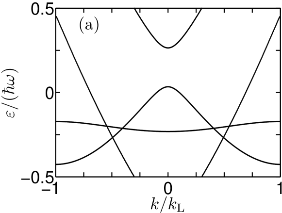
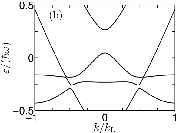
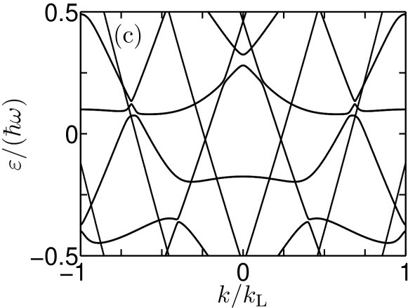
Figure 1: (a) Quasienergy spectrum of an ac-driven 1D optical lattice (67) with depth $V_{0}/E_{\rm r}=5.7$, scaled driving frequency $\hbar\omega/E_{\rm r}=3.71$, and scaled driving amplitude $K=0$. This figure is obtained by projecting the lowest three energy bands of the undriven lattice to the first quasienergy Brillouin zone, ranging from $\varepsilon/(\hbar\omega)=-1/2$ to $\varepsilon/(\hbar\omega)=+1/2$. (b) Quasienergy band structure for $K=0.5$. Here the ac Stark shifts still are comparatively weak, but the time-periodic forcing introduces pronounced avoided crossings among the “lowest” three bands. (c) Quasienergy band structure for $K=3.0$ for the “lowest” five bands, revealing substantial ac Stark shifts.

Figure 1 shows quasienergy spectra for such a 1D cosine lattice (67) with depth $V_{0}/E_{\rm r}=5.7$ under pure ac forcing, that is, for $F(t)=F_{\rm ac}\cos(\omega t)$ not containing a dc component, with driving frequency $\omega=3.71\,E_{\rm r}/\hbar$. Under the laboratory conditions specified above (⁸⁷Rb at $\lambda=842$ nm), this corresponds to $\omega/(2\pi)=12$ kHz. Figure 1(a) results when the scaled driving amplitude (50) is set to zero; this subfigure therefore is obtained by projecting the lowest three unperturbed energy bands to the fundamental quasienergy Brillouin zone, which extends from $\varepsilon=-\hbar\omega/2$ to $\varepsilon=+\hbar\omega/2$ on the ordinate. Figure 1(b) displays the quasienergy band structure for the moderate driving strength $K=0.5$; here avoided crossings show up which generally indicate multiphotonlike resonances. ArlinghausHolthaus10 Figure 1(c) then reveals pronounced ac Stark shifts (that is, shifts of the quasienergies against the zone-projected original energies) for $K=3.0$, corresponding to truly strong forcing.

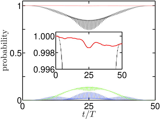
Figure 2: (Color online) Time evolution of an initial wave packet (69) under the action of a driving pulse (70) with the smooth squared-sine envelope (71), with maximum scaled amplitude $K_{\rm max}=3.0$, scaled driving frequency $\hbar\omega/E_{\rm r}=3.71$, and pulse length $T_{\rm p}=50\,T$, where $T=2\pi/\omega$ is the duration of a single cycle. The main frame shows the occupation probabilities of the original Bloch energy bands during the pulse. Apart from the initially populated lowest band $n=1$ (jagged line at the top), both bands $n=2$ and $n=3$ become significantly excited during the pulse (jagged lines at the bottom), the band $n=3$ even to a higher extent than $n=2$ at maximum driving strength. In contrast, when monitoring the same dynamics within the bases provided by the instantaneous spatiotemporal Bloch waves, only the corresponding Floquet band $n=1$ is appreciably occupied, as shown by the horizontal line at the top and magnified in the inset. Observe the scale of the inset’s ordinate!

We now turn from the quasienergy spectrum to an exemplary initial-value problem: At $t=0$ we prepare an initial wave packet (17) in the lowest Bloch band $n=1$ with a Gaussian momentum distribution,

$$g_{1}(k,0)=(\sqrt{\pi}\Delta k)^{-1/2}\exp\!\left(-\frac{k^{2}}{2(\Delta k)^{2}}\right)\;,$$ (69)

centered around $k_{\rm c}(0)/k_{\rm L}=0$ with width $\Delta k/k_{\rm L}=0.1$, and subject it to a pulse,

$$F(t)=F_{\rm max}s(t)\sin(\omega t)\;,$$ (70)

starting at $t=0$ and ending at $t=T_{\rm p}$, endowed with a smooth, squared-sine envelope function:

$$s(t)=\sin^{2}\!\left(\frac{\pi t}{T_{\rm p}}\right)\quad,\quad 0\leq t\leq T_{\rm p}\;.$$ (71)

We again set $\omega=3.71\,E_{\rm r}/\hbar$, as in Fig. 1; adjust the pulse length to 50 cycles; $T_{\rm p}=50\times 2\pi/\omega$, and fix the maximum driving amplitude $F_{\rm max}$ such that $K_{\rm max}=F_{\rm max}a/(\hbar\omega)=3.0$, corresponding to the conditions reached in Fig. 1(c). We then monitor the resulting wave-packet dynamics both in the basis of the unperturbed energy bands and in the bases provided by the instantaneous spatiotemporal Bloch waves, that is, in the family of Floquet bases which are obtained when the driving amplitude is kept fixed at any value $F_{\rm ac}=F_{\rm max}s(t_{0})$ reached during the pulse. Figure 2 displays the results: The jagged lines in the main frame show the occupation probabilities of the lowest three unperturbed Bloch bands $n=1,2$, and 3; in the middle of the pulse the band $n=3$ contains even more population than the band $n=2$. On the other hand, the horizontal line at the top depicts the occupation of the instantaneous Floquet band emerging from the lowest Bloch band: This Floquet band contains practically all the population during the entire pulse, which means that the wave function adjusts itself adiabatically to the changing morphology of its quasienergy band, ArlinghausHolthaus10 as previously sketched in Fig. 1, when the driving amplitude $F_{\rm max}s(t)$ is first increased and then decreased back to zero. To quantify the precise degree of adiabatic following, the inset in Fig. 2 shows the variation of the Floquet band population on a much finer scale. Observe that the final adiabaticity defect is on the order of merely $0.1\%$, even though the driving amplitude reaches its fairly high maximum strength within no more than 25 cycles.

With respect to the concepts developed in Sec. II, Fig. 2 strikingly demonstrates the advantages of the Floquet picture over the traditional crystal-momentum representation for the situation considered. If there were an additional probe force, its effect would have to be tediously disentangled from the fast oscillations of the Bloch band populations. When the same dynamics are seen from the Floquet viewpoint, essentially “nothing” happens, because practically all inter-Bloch-band transitions are already accounted for by continuously adapting the Floquet basis, so that the action of a probe force would stand out most clearly. Although, of course, the crystal-momentum representation is mathematically equivalent to the Floquet picture, there is no question which one is preferable here. Note also that Fig. 2 answers one further pertinent question: How do we prepare a wave packet which occupies merely a single quasienergy band, although it is undergoing rapid transitions between several Bloch bands at the same time? The recipe for achieving this is simple: Start with a wave packet occupying a single Bloch band and switch on the driving force smoothly thereby enabling adiabatic following.

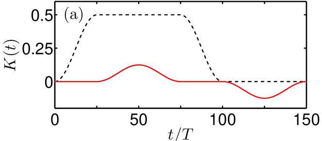
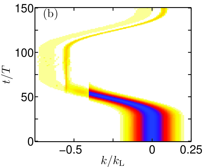
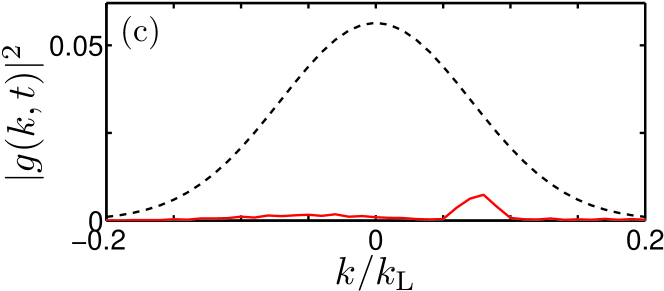
Figure 3: (Color online) (a) Protocol for achieving almost complete interband population transfer in a dressed optical lattice by means of a weak probe force. The dashed line is the scaled envelope of the dressing ac force. The solid line is the negative, scaled probe force, amplified by a factor of 10. (b) Resulting wave-packet dynamics in the Floquet representation, shown as a contour plot of $|g_{1}(k,t)|^{2}$. Under the first action of the probe force the wave packet is shifted in accordance with the generalized acceleration theorem (32), until it undergoes Zener-type transitions to other quasienergy bands at the avoided crossings visible in Fig. 1(b). After the dressing force is switched off, the second, reversed action of the probe force shifts the remaining part of the packet back to the Brillouin zone center. (c) Comparison of the initial wave packet (dashed line) with the part of the wave function that remains in the lowest energy band at the end of the process (solid line).

At this point an important issue needs to be stressed: The concept of adiabatic following, or parallel transport in a differential-geometric language, usually is applied to energy eigenstates; Simon83 ; Berry84 in the context of optical lattices this has been exploited, e.g., by Fratalocchi and Assanto for studying nonlinear adiabatic evolution and emission of coherent Bloch waves. FratalocchiAssanto07 In contrast, here we consider adiabatic following of explicitly time-dependent quasienergy eigenstates, that is, of solutions to the quasienergy eigenvalue equation (13); this is what allows us to separate the fast, oscillating time dependence of the driving force from the slow, parametric time dependence of its envelope.

Having learned these lessons, we now set the generalized acceleration theorem (32) to work. Suppose that we are prompted to empty the ground-state energy band. Starting again from an initial wave packet (69), we then may proceed as follows: First we smoothly turn on an ac force which dresses the lattice, creating avoided quasienergy crossings initially not “seen” by the adiabatically following packet. For instance, we may wish to utilize the avoided crossings showing up in Fig. 1(b). To this end, we again take an ac force with frequency $\omega=3.71\,E_{\rm r}/\hbar$ and fix its scaled driving amplitude at the plateau value $K=0.5$. This dressing force is switched on during 25 cycles with half a squared-sine envelope, maintained at maximum amplitude for 50 further cycles, and switched off again for another 25 cycles, as sketched in Fig. 3(a). If this were all we did, the wave packet would simply undergo adiabatic evolution and finally restore its initial condition, as previously observed in Fig. 2. Instead, once the maximum dressing amplitude has been reached, we now apply an additional weak probe force $F_{\rm p}(t)$ in order to exploit Eq. (32) for moving the packet away from the Brillouin zone center, driving it over the avoided crossings that have opened up in Fig. 1(b). This probe force is implemented in the form of two smooth, squared-sine shaped dc pulses, one acting during the plateau of the dressing pulse, the other acting with reversed sign after the dressing pulse is over, as drawn in Fig. 3(a). The maximum strength of the probe force here is only 2.5% of that of the dressing force; for better visibility, the probe force is magnified in Fig. 3(a) by a factor of 10.

It is now almost obvious how to describe the response of the wave packet within the Floquet picture: The initial state (69) first is adiabatically shifted into a single quasienergy-band packet during the turn-on of the dressing force. In contrast to a crystal-momentum representation, all dressing-induced fast oscillations are taken out of the dynamics of $g_{1}(k,t)$ in the Floquet representation, as shown in Fig. 3(b). When the first probe pulse acts at constant dressing amplitude, it forces the wave packet over the avoided crossing seen in Fig. 1(b), so that the packet undergoes Zener-type transitions to “higher” quasienergy bands, Zener34 ; ArlinghausHolthaus10 splitting into individual subpackets associated with the different quasienergy bands involved. When the dressing force is switched off, each of these subpackets moves adiabatically on its own quasienergy surface, finally reaching the continuously connected Bloch bands. The second, reversed probe pulse, applied after the dressing pulse is over, then acts in accordance with Bloch’s original acceleration theorem (1), shifting the various subpackets back to the Brillouin zone center. In the scenario displayed in Fig. 3, the lowest band is almost entirely depopulated by the probe-induced Zener transitions, so that only a marginal fraction of the initial packet returns, as depicted in Fig. 3(c). Thus, the main part of the initial packet has been placed in higher Bloch bands, as intended. We have also checked by explicit calculation that without the comparatively weak probe pulses the returning wave packet would be almost identical to the initial one.

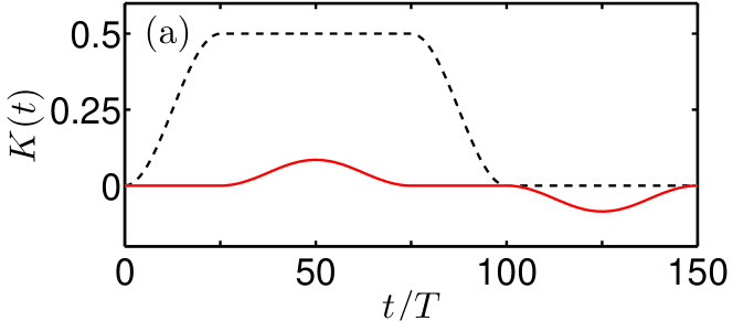
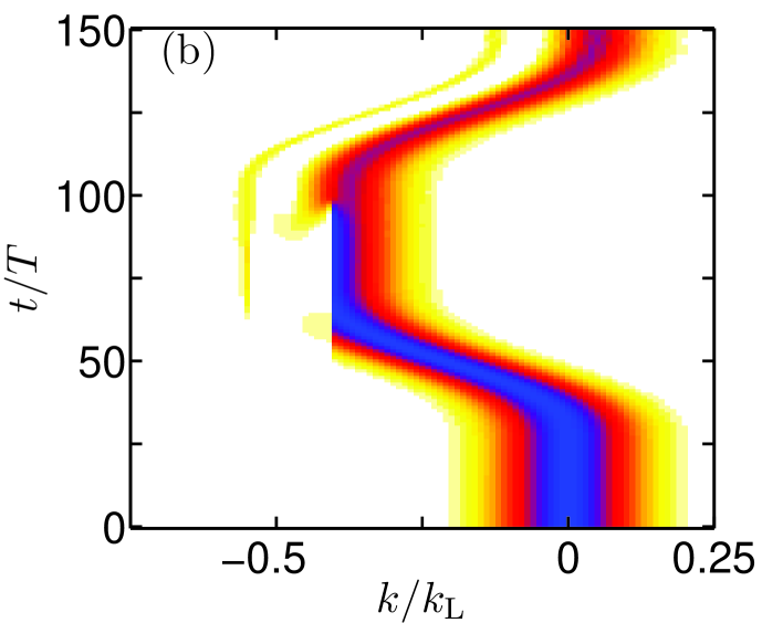
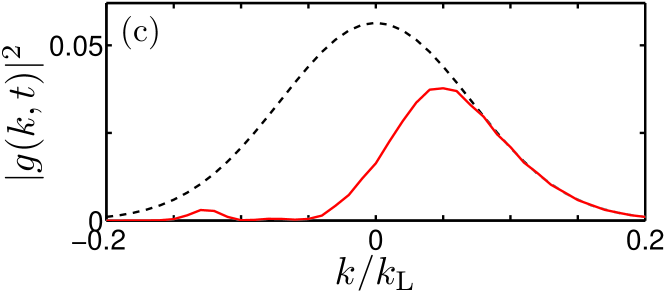
Figure 4: (Color online) (a) Protocol for achieving partial interband population transfer in a dressed optical lattice by means of a weak probe force. The dashed line is the scaled envelope of the dressing ac force, which is the same as in Fig. 3. The solid line is the negative, scaled probe force, amplified by a factor of 10; this force is weaker than the one in Fig. 3. (b) Resulting wave-packet dynamics in the Floquet representation, shown as a contour plot of $|g_{1}(k,t)|^{2}$. Under the first action of the probe force the wave packet is shifted in accordance with the generalized acceleration theorem (32), but not as far as in Fig. 3, such that it undergoes only partial Zener transitions. After the dressing force is switched off, the second, reversed action of the probe force shifts the remaining part of the packet back to the Brillouin zone center. (c) Comparison of the initial wave packet (dashed line) with the part of the wave function that remains in the lowest energy band at the end of the process (solid line).

The above example of our “dressing and probing” strategy immediately lends itself to a host of further modifications and extensions. To give but one further instance, if the probe pulse is still weaker, such that the wave packet does not pass over the avoided-crossing regime, but rather stops there, the Zener transitions are incomplete, so that a signifcant part of the initial state is recovered when the process is over. This is elaborated in Fig. 4 with the same dressing force as above, but now the maximum strength of the probe force amounts to only 1.7% of that of the dressing force. The final subpacket still occupying the lowest Bloch band then is no longer centered around $k/k_{\rm L}=0$, implying that this subpacket will move over the lattice. In a sense, the left wing of the initial wave packet has been cut out, so that Fig. 4 may be regarded as a particular paradigm of “wave-packet surgery.” ArlinghausHolthaus11

VI Conclusions

Summarizing our line of reasoning, we have introduced in Sec. II a representation of wave packets of quantum particles in spatially periodic lattices subjected to homogeneous, time-periodic forcing which is based on an expansion with respect to spatiotemporal Bloch waves and reduces to the standard crystal-momentum representation when the forcing is turned off. It embodies forcing-induced oscillations into the basis, so that only the actually relevant dynamics remain to be dealt with. Within this Floquet representation one encounters many features already familiar from solid-state physics in time-independent lattice potentials, but here their scope is different. As a prominent example, the generalized acceleration theorem derived in Sec. III takes the same form as its historic antecessor formulated by Bloch, Bloch28 but applies to single quasienergy band dynamics, which can be drastically different from single energy band behavior. There are further features which can be carried over from the crystal-momentum representation to the Floquet picture and acquire a modified meaning there, such as the expression for the group velocity of a wave packet or Zener transitions among different bands.

The super Bloch oscillations considered in Sec. IV provide a mainly pedagogical example which can be worked out in full detail analytically. Here the Floquet picture cannot exert its full strength, because one assumes a priori that the driving force does not induce transitions from the initially occupied energy band to other ones, so that the historic acceleration theorem remains capable of describing the entire dynamics. The Floquet approach leads to exactly the same result, but implies a different viewpoint, separating the dc component of the force into one part which is resonant with the ac component, and together with the latter dresses the lattice, creating a quasienergy band; the remaining residual part of the dc force then probes this new quasienergy band, rather than the original unperturbed energy band.

This theme of “dressing and probing” also prompts far-reaching strategies for achieving coherently controlled interband population transfer and even more. Two basic examples for this have been discussed in Sec. V, but the possibilities obviously extend much farther. Utilizing the generalized acceleration theorem, an initial wave packet may by split coherently into two components at an avoided quasienergy band crossing in a dressed lattice, and the lattice may then be redressed (that is, exposed to an ac force with different parameters) such that another quasienergy band structure is generated, possibly involving avoided crossings which affect only one of the daughter wave packets created in the first step, but not the other. Moreover, daughter wave packets can be made to move, possibly into different directions, and to interfere with other wavelets having been manipulated separately before in distant parts of the lattice. This vision apparently will be hard to realize with traditional solids, but it has come into immediate reach in current laboratory experiments with weakly interacting Bose-Einstein condensates in driven optical lattices. Seen against this background, the generalized acceleration theorem almost provides a blueprint for a wave-packet processor.

- (1) F. Bloch, Z. Phys. 52, 555 (1929).
- (2) N. W. Ashcroft and N. D. Mermin, Solid State Physics (Harcourt, Fort Worth, 1976), Chap. 12.
- (3) C. Kittel, Quantum Theory of Solids, 2nd ed. (Wiley, New York, 1987).
- (4) H. G. Roskos, M. C. Nuss, J. Shah, K. Leo, D. A. B. Miller, A. M. Fox, S. Schmitt-Rink, and K. Köhler, Phys. Rev. Lett. 68, 2216 (1992).
- (5) J. Feldmann, K. Leo, J. Shah, D. A. B. Miller, J. E. Cunningham, T. Meier, G. von Plessen, A. Schulze, P. Thomas, and S. Schmitt-Rink, Phys. Rev. B 46, 7252 (1992).
- (6) J. Feldmann, Bloch Oscillations in a Semiconductor Superlattice, in Festkörperprobleme, Advances in Solid State Physics Vol. 32, edited by U. Rössler (Vieweg, Braunschweig/Wiesbaden, 1992), p. 81.
- (7) C. Waschke, H. G. Roskos, R. Schwedler, K. Leo, H. Kurz, and K. Köhler, Phys. Rev. Lett. 70, 3319 (1993).
- (8) A. A. Ignatov, E. Schomburg, K. F. Renk, W. Schatz, J. F. Palmier, and F. Mollot, Ann. Physik 3, 137 (1994).
- (9) J. Rotvig, A.-P. Jauho, and H. Smith, Phys. Rev. Lett. 74, 1831 (1995).
- (10) A. A. Ignatov, E. Schomburg, J. Grenzer, K. F. Renk, and E. P. Dodin, Z. Phys. B 98, 187 (1995).
- (11) A. M. Bouchard and M. Luban, Phys. Rev. B 52, 5105 (1995).
- (12) K. Unterrainer, B. J. Keay, M. C. Wanke, S. J. Allen, D. Leonard, G. Medeiros-Ribeiro, U. Bhattacharya, and M. J. W. Rodwell, Phys. Rev. Lett. 76, 2973 (1996).
- (13) V. G. Lyssenko, G. Valušis, F. Löser, T. Hasche, K. Leo, M. M. Dignam, and K. Köhler, Phys. Rev. Lett. 79, 301 (1997).
- (14) G. Lenz, I. Talanina, and C. M. de Sterke, Phys. Rev. Lett. 83, 963 (1999).
- (15) M. Ben Dahan, E. Peik, J. Reichel, Y. Castin, and C. Salomon, Phys. Rev. Lett. 76, 4508 (1996).
- (16) O. Morsch, J. H. Müller, M. Cristiani, D. Ciampini, and E. Arimondo, Phys. Rev. Lett. 87, 140402 (2001).
- (17) H. Jones and C. Zener, Proc. R. Soc. Lond. A 144, 101 (1934).
- (18) C. Zener, Proc. R. Soc. Lond. A 145, 523 (1934).
- (19) J. Callaway, Quantum Theory of the Solid State (Academic Press, New York, 1976).
- (20) M. Holthaus, Z. Phys. B 89, 251 (1992).
- (21) K. Drese and M. Holthaus, Chem. Phys. 217, 201 (1997).
- (22) S. Arlinghaus and M. Holthaus, Phys. Rev. A 81, 063612 (2010).
- (23) J. Zak, Phys. Rev. Lett. 71, 2623 (1993).
- (24) V. Grecchi and A. Sacchetti, Phys. Rev. B 63, 212303 (2001).
- (25) B. Simon, Phys. Rev. Lett. 51, 2167 (1983).
- (26) M. V. Berry, Proc. R. Soc. Lond. A 392, 45 (1984).
- (27) H. Sambe, Phys. Rev. A 7, 2203 (1973).
- (28) E. Haller, R. Hart, M. J. Mark, J. G. Danzl, L. Reichsöllner, and H.-C. Nägerl, Phys. Rev. Lett. 104, 200403 (2010).
- (29) A. R. Kolovsky and H. J. Korsch, J. Sib. Fed. Univ.: Math. Phys. 3, 311 (2010); arXiv:0912.2587.
- (30) A. Alberti, V. V. Ivanov, G. M. Tino, and G. Ferrari, Nat. Phys. 5, 547 (2009).
- (31) K. Kudo and T. S. Monteiro, Phys. Rev. A 83, 053627 (2011).
- (32) W. Kohn, Phys. Rev. 115, 809 (1959).
- (33) W. V. Houston, Phys. Rev. 57, 184 (1940).
- (34) A. Eckardt, M. Holthaus, H. Lignier, A. Zenesini, D. Ciampini, O. Morsch, and E. Arimondo, Phys. Rev. A 79, 013611 (2009).
- (35) M. Grifoni and P. Hänggi, Phys. Rep. 304, 229 (1998).
- (36) S. Longhi, Phys. Rev. A 71, 065801 (2005).
- (37) K. Kudo, T. Boness, and T. S. Monteiro, Phys. Rev. A 80, 063409 (2009).
- (38) A. Zenesini, H. Lignier, D. Ciampini, O. Morsch, and E. Arimondo, Phys. Rev. Lett. 102, 100403 (2009).
- (39) A. Eckardt, P. Hauke, P. Soltan-Panahi, C. Becker, K. Sengstock, and M. Lewenstein, EPL 89, 10010 (2010).
- (40) J. Struck, C. Ölschläger, R. Le Targat, P. Soltan-Panahi, A. Eckardt, M. Lewenstein, P. Windpassinger, and K. Sengstock, Science Express, published online 21 July 2011 [DOI:10.1126/science.1207239]
- (41) O. Morsch and M. Oberthaler, Rev. Mod. Phys. 78, 179 (2006).
- (42) I. Bloch, J. Dalibard, and W. Zwerger, Rev. Mod. Phys. 80, 885 (2008).
- (43) A. Fratalocchi and G. Assanto, Phys. Rev. A 75, 013626 (2007).
- (44) S. Arlinghaus and M. Holthaus (unpublished).