Noninvasiveness and time symmetry of weak measurements

Abstract

Measurements in classical and quantum physics are described in fundamentally different ways. Nevertheless, one can formally define similar measurement procedures with respect to the disturbance they cause. Obviously, strong measurements, both classical and quantum, are invasive – they disturb the measured system. We show that it is possible to define general weak measurements, which are noninvasive: the disturbance becomes negligible as the measurement strength goes to zero. Classical intuition suggests that noninvasive measurements should be time symmetric (if the system dynamics is reversible) and we confirm that correlations are time-reversal symmetric in the classical case. However, quantum weak measurements – defined analogously to their classical counterparts – can be noninvasive but not time symmetric. We present a simple example of measurements on a two-level system which violates time symmetry and propose an experiment with quantum dots to measure the time-symmetry violation in a third-order current correlation function.

1 Introduction

The notion of a noninvasive measurement – a measurement that does not disturb the system being measured – is undisputed in classical physics because one can assign a real physical value to every point in phase space at all times. Even so, the situation becomes complicated if we introduce explicit detectors since these may disturb the system. In quantum physics, the notion of a noninvasive measurement is always problematic [1]. One cannot assign a value to an observable without discussing the measurement procedure. Strong projective measurements [2] (and therefore the majority of general measurements [3, 4]) are certainly invasive.

A good candidate for a noninvasive measurement scheme is a weak measurement [5]. In general, by reducing the coupling of the detector system to the system under measurement, the invasiveness is reduced at the price of an increased detector noise. This leads to paradoxes of unusually large values for single measurement results after a subsequent postselection [5], or a quasiprobability for the measured distribution after the detector noise has been removed[6]. There is growing interest in such measurements [7, 8, 9, 10, 11].

In this paper, we answer the question of when our intuitive criteria (defined below) of noninvasiveness and time symmetry of measurements are satisfied, for both classical and quantum cases. Time-reversal symmetry of observables is a fundamental symmetry of physics, valid in classical physics and in general – because it is a good symmetry of quantum electrodynamics – in low-energy physics (in high-energy physics combined with parity and charge conjugation). This symmetry is generally probed by the measurement of single, non-time-resolved measurements, such as the measurement of electric dipole moments of particles. However, time-reversal symmetry also constrains the results of time-resolved measurements with multiple measurements. For such considerations, one must consider the invasiveness of the measurements themselves which will tend to break time-reversal symmetry.

1.1 Measurement Schemes

A measurement scheme is a description of how to measure observables—functions of phase space for classical physics or Hermitian operators for quantum physics. A measurement takes place on a system under measurement which is a member of the ensemble under measurement. As usual, systems of the ensemble are considered to be identically distributed and statistically independent. Returning to the measurement scheme, it should be a description of (a) what the detector system is and how it is prepared, (b) how the detector system is coupled to the system under measurement, and (c) how the detector system is itself measured, and how the measured value is interpreted. The measurement scheme, essentially a description of the detectors, should be generally independent of the ensemble under measurement, and only (b), the coupling to the system of interest, should depend on the observable. Also, the measurement of the detector system must be defined in terms of axioms—both classical and quantum (e.g. by projection postulate). The measurement result should contain the inherent statistical distribution $Q$ of the measured system. The measurement result also contains detector noise $D$ resulting, in an similar fashion, from the statistical and quantum properties of the detector system. By the measurement of many systems from an ensemble, the probability distribution $P$ of the measurement can itself be measured. The detector noise probability distribution $D$ of a null measurement—a ‘measurement’ where the detector system is prepared but not coupled to the system under measurement—can be determined. We postulate that the measurement scheme is expressed by a convolution, $P=Q\ast D$ and in this case the detector noise may be removed by deconvolution. The measurement schemes considered in this paper all possess this last property.

1.2 Noninvasiveness of measurements

We consider time-resolved measurements of observables $A_{1},\dots,A_{n}$ measured at times $t_{1},\dots,t_{n}$, with outcomes $a_{1},\dots,a_{n}$ occurring with probabilities $Q(a_{1},\dots,a_{n})$. The probability density $Q$ contains all the information about the experiment and we formulate criteria for noninvasiveness and time symmetry in terms of $Q$, or more exactly, by requiring equality between $Q$ values measured in different experiments.

An arbitrary operation is non-disturbing if the probability density of other measurements is unchanged by the test operation’s addition or removal. In other words, integrating over the single measurement should yield the same distribution that would be obtained if that measurement were never performed. Therefore, our criterion of noninvasiveness of the $k$th measurement reads

$$\int\rmd a_{k}Q(a_{1},\ldots,a_{n})=Q(a_{1},\ldots,\displaystyle{\not}a_{k},\ldots,a_{n}).$$ (1)

Equation (1) equates probabilities between two different experiments. In the first, the $k$th measurement is integrated out and in the second, the slash notation indicates that the variable was not measured at all. This defines noninvasiveness of single measurements on a given experiment.

More generally, if new measurements of observables $A_{k_{1}},\dots,A_{k_{m}}$ can be inserted at intermediate times without changing the previous probability density as in (1) then the all of them are noninvasive. The noninvasiveness is stronger if (1) is satisfied for a fixed $A_{k}$ but arbitrary other measurements.

1.3 Time symmetry of measurements

We assume that time reversal is a good symmetry for the equations of motion of the system and investigate whether this leads to a corresponding symmetry expressed in the results of measurements performed on the system. We should note that time reversal symmetry holds only for nondissipative, Hamiltonian systems. However, physical dissipation is always a result of ignoring fast-changing and fine-grained degrees of freedom, often modeled by a heat bath coupled weakly to the system. If one had access to all the degrees of freedom and the heat bath, one could reverse the full phase space probability and restore time symmetry. Even if it is not practically possible to reverse fine-grained degrees of freedom, an alternate solution is to restrict ourselves to states in equilibrium coupled to a heat bath, which are time-symmetric themselves in the thermodynamic limit.

To express the expected time-reversal symmetry of a set of measurements, we begin by denoting the time-reversed version of an object $X$ by $X^{T}$, i.e., position: $q^{T}=q$ and momentum $p^{T}=-p$. The time-reversed experiment involves the time reversed initial state $\rho\to\rho^{T}$, time-reversed measured quantities $A\to A^{T}$ with results $a\to a^{T}$, and also reversed time—and therefore, ordering—of the measurements. Hence, for the probability $Q$, our criterion of time symmetry of measurements reads

$$Q(a_{1}(t_{1}),\ldots,a_{n}(t_{n}))=Q^{T}(a^{T}_{n}(-t_{n}),\ldots,a^{T}_{1}(-t_{1})),$$ (2)

where we compare the probability densities of the forward ($Q$) and reversed ($Q^{T}$) sets of measurements. In such a form, classically (2) holds for equilibrium and non-equilibrium systems and is independent of the validity of charge conjugation and parity symmetries and also of relativistic invariance [12, 13, 14]. When fulfilled—assuming for the moment that the measurements are non-invasive—the result (2) leads to the principle of detailed balance[15] and reciprocity of thermodynamic fluxes [16].

1.4 Main result

The above criteria (1) and (2) must be confronted with real detection protocols. For each measurement, there is a detection protocol that includes some interaction between the original system and an ancilla that is later decoupled with the imprinted information retrieved from the system. We should add the remark that the internal dynamics of the detector may be irreversible, but this is irrelevant, because we ask only about the behavior of the system. Note also that, for the time symmetry to hold, the measurements should not disturb the system in the sense of the criterion (1), since any disturbance would create an asymmetry between before and after the measurement.

The majority of measurements are invasive and irreversible, both classical and quantum. However, there exists a special class of measurements, defined both classically and quantum mechanically, which are noninivasive under certain conditions. They are described by an instantaneous interaction between the system and detector $\sim gpA$, where $A$ is the measured observable, $p$ is the detector’s momentum and $g$ is the coupling strength (see details later in the text). The initial state of the detector is the zero mean Gaussian. The observer finally registers the position which is shifted by $gA$. The result contains also the internal detection noise, which is subtracted/deconvoluted. For all finite $g$ the scheme is invasive, except if the observables are compatible (vanishing Poisson bracket or commutator) or if initially $p=0$, which makes sense only classically (we do not want divergent position).

However, the scheme becomes noninvasive (both classically and quantum) in the limit $g\to 0$, while rescaling the detector’s result by $1/g$ – this is the weak measurement [5]. Surprisingly, classical and quantum weak measurements differ with respect to time symmetry (2). The behavior of different types of measurements is summarized in Table 1. The aim of this paper is to explain the origin of this difference between classical and quantum measurements. We will also show the asymmetry explicitly by giving an example of a measurement of a simple two-level system and propose an experimentally feasible realization by charge measurements on a quantum dot connected to a reservoir.

	Noninvasiveness	Time symmetry
General, strong	No	No
Classical $p=0$ (arbitrary $g$)	Yes	Yes
Compatible (arbitrary $g$)	Yes	Yes
Classical weak ($g\to 0$)	Yes	Yes
Incompatible quantum weak ($g\to 0$)	Yes	No
Quantum weak ($g\to 0$) – exceptions	Yes	Yes

Table 1: Different types of measurements may satisfy noninvasiveness and/or time symmetry. The exceptions include position and/or momentum measurement in a simple harmonic oscillator, two-time correlations and other accidental symmetries or quasiclassical systems.

2 Time symmetry violation

We will show in next sections that in the classical weak measurement limit one can find

$$Q(a)=\langle\delta(a_{n}-A_{n}(t_{n}))\cdots\delta(a_{1}-A_{1}(t_{1}))\rangle,$$ (3)

where the average $\langle\cdots\rangle=\int\rmd\Gamma\cdots\rho$ is taken in the initial state $\rho$ in the phase space $\Gamma$ and $A(t)$ denotes a classical analogue of the Heisenberg picture for the observable $A$. This clearly satisfies noninvasiveness and time symmetry, because $A$ are commuting numbers and we can reorder them under time reversal.

Now, in the quantum case, we will get

$$Q(a)=\langle\delta(a_{n}-\check{A}_{n}(t_{n}))\cdots\delta(a_{1}-\check{A}_{1}(t_{1}))\rangle$$ (4)

for $t_{n}\geq\cdots\geq t_{2}\geq t_{1}$, where $\langle\cdots\rangle=\mathrm{Tr}\cdots\rho$ with the initial density matrix $\rho$. The superoperators act as $\check{A}B=(AB+BA)/2$, for the observable operator $A$. This quantity is no longer a probability but a quasiprobability [6] and still satisfies noninvasiveness (1). However, the time symmetry (2) is violated, except for compatible measurements (e.g. space-like separated[12]). Mathematically, this is because we replace the classical $c$-number multiplication (obviously a commuting operation) by the quantum anticommutator of operators (therefore noncommuting). We cannot reorder superoperators $\check{A}$ under time reversal.

For slow measurements, each operator $A(t)$ in (4) is replaced with $\int f(t)A(t)\rmd t$, where $f(t)$ turns on and off slowly compared to relevant timescales of the system. This slow measuring smoothes the resulting distribution $Q$ so that any antisymmetric contributions vanish and therefore time symmetry (2) will still apply. Roughly speaking, the more classical is the system, the more time-symmetric it is.

The time symmetry (2) can be tested by comparing moments of the distribution,

$$\langle{a_{1}(t_{1})\cdots a_{n}(t_{n})}\rangle_{Q}=\langle{a^{T}_{n}(-t_{n})\cdots a^{T}_{1}(-t_{1})}\rangle^{T}_{Q}.$$ (5)

We emphasize that the quantities in (5) are expectation values of products of measurement results, and should not be confused with expectation values of observables in an ensemble. The ordering of $a_{1}$ to $a_{n}$ is mathematically irrelevant, but serves as a reminder of the ordering of measurements in the experiment.

Linear correlations of quantum weak measurements—in the limit of zero measurement strength—are given by [6, 19]

$$\left\langle\prod_{k}a_{k}(t_{k})\right\rangle_{Q}=\langle\check{A}_{n}(t_{n})...\check{A}_{2}(t_{2})\check{A}_{1}(t_{1})\rangle$$ (6)

We can freely permute the $a$ in the left hand side but not the $\check{A}$ in the right hand side (they do not commute and the order reflects that $t_{n}\geq\cdots\geq t_{2}\geq t_{1}$). This asymmetry is only present for fast measurements of three or more incompatible observables. This does not need a specific system. In contrast, only specific systems and observables do not show the asymmetry; one such an exception is e.g. position measurement in a simple harmonic oscillator. In the case of compatible or only two (not necessarily compatible) measurements the ordering is irrelevant and the symmetry (5) holds.

3 Direct measurements

Let us take a classical system with the probability density $\rho(\Gamma)$ in phase space $\Gamma=(\Gamma_{1},\dots,\Gamma_{N})$ with $\Gamma_{i}=(q_{i},p_{i})$ being a pair of canonical generalized position and momentum. The evolution is given by the Hamiltonian $H(\Gamma)$ and can be expressed compactly using the Liouville operator $\check{L}$, defined by $\check{L}A=(A,H)$ where

$$(A,B)=\sum_{i}\left[\frac{\partial A}{\partial q_{i}}\frac{\partial B}{\partial p_{i}}-\frac{\partial B}{\partial q_{i}}\frac{\partial A}{\partial p_{i}}\right]$$ (7)

is the Poisson bracket. One has $\partial_{t}\rho=-\check{L}\rho$ or $\rho(t)=\rme^{-t\check{L}}\rho(0)$.

Let us consider a direct sequential measurement of quantities $A_{1}\dots A_{n}$ measured at times $t_{1}<t_{2}<\dots<t_{n}$, with the results $a_{1}\dots a_{n}$, respectively. The probability distribution is naturally postulated as

$$Q(a)=\int\rmd\Gamma\delta(a_{n}-A_{n})\rme^{(t_{n-1}-t_{n})\check{L}}\cdots$$

$$\delta(a_{2}-A_{2})\rme^{(t_{1}-t_{2})\check{L}}\delta(a_{1}-A_{1})\rme^{-t_{1}\check{L}}\rho(0).$$ (8)

Alternatively, it can be written as

$$Q(a)=\int\rmd\Gamma\delta(a_{n}-A_{n}(t_{n}))\cdots\delta(a_{1}-A_{1}(t_{1}))\rho(0)$$ (9)

where $A(t)=\rme^{t\check{L}}A$. The above quantity coincides with (3), is positive and normalized so it is a normal probability. As we already noted, it satisfies noninvasiveness (1) and time symmetry (2).

Now, the quantum direct measurement is governed by the projection postulate [2]. It is obviously invasive, violates (1) and (2), which is not at all surprising. Looking for quantum noninvasiveness, we have to abandon direct measurements [3]. Since we want to compare classical and quantum noninvasive measurements, we will consider indirect measurements both classical and quantum.

4 Weak measurements

Let us now construct a model of a weak measurement which functions both classically and quantum mechanically[5]. We have no direct access to the quantity $A$ at time $t_{0}$ but we couple a detector for an instant. The interaction Hamiltonian, added to the system, reads $H_{I}=g\delta(t-t_{0})pA$ where $p$ is the detector’s momentum, and $g$ is the measurement’s strength. We will use a very compact notation that highlights quantum-classical analogies and differences. This is why many formulae below apply both to classical and quantum cases, with differences only in the mathematical objects (e.g. numbers or operators, phase-space density or density matrix, operator or superoperator). The quantum Liouville superoperator reads $\check{L}A=[A,H]/\rmi\hbar$ (commutator $[A,B]=AB-BA$). As in the classical evolution of phase space density, operators in the Heisenberg picture evolve as $A(t)=\rme^{t\check{L}}A$. For a single measurement, the total initial state is a product $\rho_{\rmd}\rho(t_{0})$, where $\rho_{\rmd}$ is the state of the detector. After the measurement, the total density is

$$\rho_{\rmd}\rho(t_{0})\to\exp(g(\check{A}\check{p}^{q}+\check{p}\check{A}^{q}))\rho_{\rmd}\rho(t_{0}),$$ (10)

where classically $\check{A}=A$ (multiplication by $A$), quantum-mechanically $\check{A}B=\{A,B\}/2$ (anticommutator $\{A,B\}=AB+BA$), and the (super)operator $\check{A}^{q}$ is given classically by $\check{A}^{q}B=(A,B)$, and quantum mechanically by $\check{A}^{q}B=[A,B]/\rmi\hbar$. For a more conventional approach, see Appendix A. Note that classically $\check{p}^{q}=-\partial_{q}$ for the canonically conjugated $q$. The analogy between classical Poisson brackets and quantum commutators was recognized in the early days of quantum mechanics [20]. The novel analogy here is between the classical multiplication by an observable and the quantum anticommutator. The fact that we replace a (commuting) number by a (noncommuting) superoperator helps to understand why quantum weak measurements do not obey time symmetry while classical weak measurements do.

If we discard the results of the measurement then the resulting density reads $\langle\exp(gp\check{A}^{q})\rho\rangle$, where the average denotes $\int\rmd\Gamma_{\rmd}\cdots\rho_{\rmd}$ classically and $\mathrm{Tr}_{\rmd}\cdots\rho_{\rmd}$ quantum mechanically (subscript $\rmd$ denotes detector’s subspace). The procedure can be repeated for sequential measurements as depicted in figure 1.

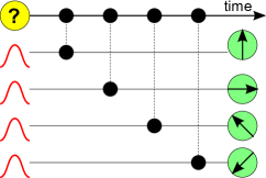
Figure 1: A schematic diagram of weak measurements, analogous to figure 3 in [9]. The measured system (yellow) instantly interacts with a prepared ancilla (red state), which is measured (projectively in the quantum case) afterwards (green detector). The procedure is repeated with identical but independent ancillae.

We take the initial state of the detector given by

$$\rho_{\rmd}\propto\exp(-q^{2}/2\alpha-p^{2}/2\beta)$$ (11)

where $q,p$ are a pair of conjugate canonical observables (with the property $(q,p)=1$ or $[q,p]=\rmi\hbar$). This is a generic symmetric Gaussian state. If measured classically the initial variances read $\langle q^{2}\rangle\equiv\sigma_{q}=\alpha$ and $\langle p^{2}\rangle\equiv\sigma_{p}=\beta$. Quantum mechanically (under projective measurement) $\sigma_{q}=(\hbar/2)\sqrt{\alpha/\beta}\coth\sqrt{\hbar^{2}/4\alpha\beta}$ and $\sigma_{p}=(\hbar/2)\sqrt{\beta/\alpha}\coth\sqrt{\hbar^{2}/4\alpha\beta}$. Note that for $\alpha\beta\gg\hbar^{2}$ they reduce to the classical result while $\sigma_{q}\sigma_{p}\geq\hbar^{2}/4$ is imposed by the Heisenberg uncertainty principle.

We register directly the value of $q$. However, the way of measuring of $q$ is in principle irrelevant, both classical and quantum, and may be well disturbing because the detector will not interact with the system anymore. The detector (classical or quantum) can evolve irreversibly, we are only interested in the data extracted from the system.

We apply a sequence of such measurements, using identical, independent detectors $q_{1},\dots,q_{n}$, but coupled at different times to possibly different observables. It is convenient to define a result-conditioned density $\rho_{g}(q)$, normalized by the final result-integrated density $\rho_{g}=\int\rmd^{n}q\;\rho_{g}(q)$. The probability density of a given sequence of results is given by $P(q)=\int\rmd\Gamma\rho_{g}(q)$ or $\mathrm{Tr}\rho_{g}(q)$. Now, $\rho_{g}(a)$ is given by

$$\rho_{g}(q)=\int\rmd^{n}a\;\varrho_{g}(a)\prod_{k}D(q_{k}-ga_{k}),$$ (12)

where $D$ is the zero-mean Gaussian noise with the variance $\sigma_{q}$. The quantity $\varrho_{g}(a)$ reads

$$\varrho_{g}(a)= \rme^{\sigma_{p}(g\check{A}_{n}^{q})^{2}/2}\delta(a_{n}-\check{A}_{n})\rme^{(t_{n-1}-t_{n})\check{L}}\cdots$$ (13)

$$\times\rme^{\sigma_{p}(g\check{A}_{2}^{q})^{2}/2}\delta(a_{2}-\check{A}_{2})\rme^{(t_{1}-t_{2})\check{L}}\rme^{\sigma_{p}(g\check{A}_{1}^{q})^{2}/2}\delta(a_{1}-\check{A}_{1})\rme^{-t_{1}\check{L}}\rho(0).$$

This is classically a standard probability density but not a positive definite density matrix in quantum mechanics. It is clear when defining $Q_{g}(a)=\int\rmd\Gamma\varrho_{g}(a)$ and $Q_{g}(a)=\mathrm{Tr}\varrho_{g}(a)$. Now the quantum $Q_{g}$ is only a quasiprobability [6]. One can write down the convolution relation analogous to (12),

$$P(q)=\int\rmd^{n}a\;Q_{g}(a)\prod_{k}D(q_{k}-ga_{k}).$$ (14)

Both $\varrho_{g}$ and $Q_{g}$ have a well-defined limit $g\to 0$, $\varrho\equiv\varrho_{0}$ and $Q\equiv Q_{0}$. Then (13) reduces to (8) classically. In the quantum case,

$$Q(a)=\mathrm{Tr}\delta(a_{n}-\check{A}_{n}(t_{n}))\cdots\delta(a_{1}-\check{A}_{1}(t_{1}))\rho(0)$$ (15)

with $\check{A}(t)B=\{A(t),B\}/2$ or equivalently $\check{A}(t)=\rme^{t\check{L}}\check{A}\rme^{-t\check{L}}$, which coincides with (4). The effect of disturbance (both classical and quantum!) is of the order $g^{2}$ so it vanishes in the limit $g\to 0$.

One can relate correlation functions

$$\langle q_{1}\cdots q_{n}\rangle_{P}=g^{n}\langle a_{1}\cdots a_{n}\rangle_{Q}.$$ (16)

The leading contribution to such correlation functions is of the order $g^{n}$, while the lowest correction due to disturbance is of the order $g^{n+2}$, as follows from (12) and (13).

Both classical and quantum $Q$ satisfy noninvasiveness (1), but only in the $g\to 0$ limit. There are exceptions when noninvasiveness holds for an arbitrary $g$. In particular $Q_{g}=Q$ is independent of $g$ and always a real positive probability for compatible observables – if $(A_{j}(t_{j}),A_{k}(t_{k}))=0$ classically or $[A_{j}(t_{j}),A_{k}(t_{k})]=0$ quantum mechanically for all $j,k$. We emphasize that the deconvolved result-conditioned density $\varrho(a)$ (13) changes with each measurement because it gets the factor $\delta(a-A)$ or $\delta(a-\check{A})$. This is because it must contain the read-off knowledge (it is gaining information – not disturbance). It is impossible to preserve the result-conditioned density unchanged by any measurement, both classical or quantum (unless the measurement is void) – in this sense all measurements would be invasive. Hence, only after integration it makes sense to distinguish between invasive and noninvasive measurements.

From (12) and (13) we see also that the result-integrated density after a single weak measurement gets the factor $\rme^{\sigma_{p}(g\check{A}^{q})^{2}/2}$, which reduces to identity in the limit $g\to 0$. This is why weak measurements (both classical and quantum) are noninvasive in a stronger sense: their disturbance vanishes as $g^{2}$ regardless of the type of measurements before/after. For a comparison, strong measurements of compatible observables are mutually noninvasive but we can find an incompatible observable whose results they disturb. The price of weak measurements is that one has to repeat the experiment $\gtrsim 1/g^{2}$ times to get the weak signal out of statistics.

Note also that the scaling $q\sim ga$ is analogous in the classical and quantum cas. In the classical case, however, one can take $\sigma_{p}=0$, which makes the limit $g\to 0$ unnecessary. On the other hand, the quantum mechanical uncertainty principle allows only for the limiting noninvasiveness. One could argue (both classically and quantum) that there is still some invasiveness for large results because the result-conditioned density $\rho_{g}(q)$ is affected by different factors for different values of $A$. Namely, $\exp(-(q-gA)^{2}/2\sigma_{q})/\exp(-(q-gA^{\prime})^{2}/2\sigma_{q})$ can be large even for small $g$. However, this requires $q\gtrsim q_{0}=\sigma_{q}/gA$ which happens very rarely for small $g$, with the estimated probability of the rapidly vanishing Gaussian tail $\sim\rme^{-q_{0}^{2}/2\sigma_{q}}=\rme^{-\sigma_{q}/2(gA)^{2}}$ so it is irrelevant for the discussion of noninvasiveness. Moreover, $\rho_{g}(q)$ also contains the read-off knowledge, although rescaled by $g$, while only the change of result-integrated $\rho_{g}$ is quantifies invasiveness.

4.1 Causality

One may ask whether it is possible to enforce time-symmetry (2) in any other measurements scheme. Unfortunately, we would pay a high price – abandoning causality of measurements.

All general quantum measurements appear in a causal way,

$$P(q)=\mathrm{Tr}\check{K}_{n}(q_{n})\rme^{(t_{n-1}-t_{n})\check{L}}\cdots\check{K}_{1}(q_{1})\rme^{-t_{1}\check{L}}\rho(0)$$ (17)

with normalized completely positive maps $\check{K}$ [3, 4]. Even more generally

$$P(q)=\mathrm{Tr}\mathcal{T}\check{K}[A,q]\rho,$$ (18)

where $\mathcal{T}$ denotes time ordering of superoperators that depend on observables $A(t)$ in Heisenberg picture. Now, every causal measurement of non-zero strength is disturbing (weak measurements from section 3 create a disturbance $\sim g^{2}$) but only forward in time. If we measure at $t_{1}<t_{2}<t_{3}$ then the measurement $1$ disturbs $1,2,3$, the measurement $2$ disturbs only $2,3$ and the last disturbs only itself. If there existed any measurement scheme with the time-symmetric limit (with a vanishing parameter analogous to $g$) then it would have also time-symmetric disturbance at finite strength – violating causality.

However, if we give up the above rule or are satisfied by only limiting causality (at $g=0$) we can e.g. define

$$Q(a)=\int\frac{\rmd^{n}\chi}{(2\pi)^{n}}\mathrm{Tr}\exp\sum_{k}\rmi(a_{k}-A_{k}(t_{k}))\chi_{k}\>\rho.$$ (19)

The corresponding map $\check{K}B=KBK^{\dagger}$ for $n$ measurements reads

$$K(q)=(2\pi)^{-n/4}\rme^{\sum_{k}(2gA_{k}(t_{k})q_{k}-q_{k}^{2})/4}\left[\mathcal{T}_{s}\rme^{-\left(\sum_{k}gA_{k}(t_{k})\right)^{2}/2}\right]^{1/2},$$ (20)

where $\mathcal{T}_{s}$ denotes the rule of complete symmetrization of operator products in Taylor expansion. The probability $P=\mathrm{Tr}\check{K}\rho$ is related to $Q$ by (12) with $\sigma_{q}=1$. It is perfectly time-symmetric but the disturbance is time symmetric, too, for $g>0$. In this work, we have not considered this option, because all known experimental detection schemes confirm causality.

5 Examples

5.1 Double well

Let us demonstrate the paradox in a simple system consisting of a particle in a double-well potential as in figure 2. For simplicity, we take an equilibrium state, but the asymmetry appears also in a completely general case. The particle is effectively described by the ground states of the left and right wells, $|{l}\rangle$ and $|{r}\rangle$ respectively. Higher excited states have much more energy and for low temperatures can be ignored, leaving an effective two-state system. Using the basis states, the operator for expected location is $Z=|{l}\rangle\langle{l}|-|{r}\rangle\langle{r}|$, and the effective Hamiltonian reads

$$H=\varepsilon(|{l}\rangle\langle{l}|-|{r}\rangle\langle{r}|)+\tau(|{l}\rangle\langle{r}|+|{r}\rangle\langle{l}|),$$ (21)

where $2\varepsilon$ is the energy difference between wells and $\tau$ is the tunneling amplitude.

For low-energy physics, time reversal alone is already a good symmetry in the equations of motion so, in absence external magnetic field, the equilibrium state is time symmetric. Hence, $H$ and $Z$ are even under time reversal ($H^{T}=H$, $Z^{T}=Z$). We are now in a position to test equation (5) with $z$ measured at three separate times and with the initial thermal state $\rho\propto\exp(-H/kT)$. The correlation for three weak measurements can be calculated using (6) and $Z(t)=\rme^{\rmi Ht/\hbar}Z\rme^{-\rmi Ht/\hbar}$:

$$\langle{z(t_{1})z(t_{2})z(t_{3})}\rangle=\alpha(\varepsilon^{2}+\tau^{2}\cos(2(t_{3}-t_{2})\Delta/\hbar)),$$ (22)

where $\Delta=\sqrt{\varepsilon^{2}+\tau^{2}}$, $\alpha=-(\varepsilon/\Delta^{3})\tanh(\Delta/kT)$. For this system and measurements, the expression corresponding to the right-hand side of (5) differs from (22) only by the exchange of $t_{3}-t_{2}$ with $t_{2}-t_{1}$. However, (22) is clearly asymmetric under this exchange, demonstrating that time-reversal symmetry is broken for correlations of quantum weak measurements. As a side note, it can be shown that the correlation (22) is independent of measurement strength; however, this coincidence does not hold in general.

Figure 2: The double well, described effectively by two states $|{l}\rangle$ and $|{r}\rangle$, with energy shift $2\varepsilon$ and tunneling amplitude $\tau$. Even in the ground state, quantum fluctuations allow jumps between the wells, which turn to be non-time symmetric under weak measurement.

5.2 Quantum dot

Despite the simplicity of the above example, a genuine, fast weak detection scheme is probably difficult to implement experimentally in this case. Below, we present a more realistic example, leveraging recent developments in quantum dots [21].

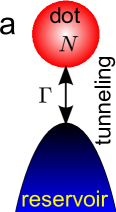
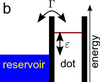
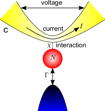
Figure 3: (a) The system consists of the dot (red) exchanging the elementary charge with a reservoir (blue). (b) The diagram of energy levels. At zero temperature, the Fermi sea of blue levels is full but electrons may still jump on and off the dot’s red level.(c) Proposed detection by an electric junction (yellow). The junction and dot are weakly coupled capacitively and the directly measured quantity is the current $I$ through the junction biased with the voltage. The charge is allowed to jump between the dot and the lower reservoir but not the junction.

We consider a quantum dot containing a single energy level $\varepsilon$, coupled to a Fermi reservoir by an energy independent coupling described effectively by the tunneling rate $\Gamma/\hbar$, as depicted in figures 3(a) and (b). The occupation $n$ on the dot (classically either $0$ or $1$ in elementary charge units) is the measured observable $N$. The quantum observable and the Hamiltonian read [22]

$$N=c^{\dagger}c,\>H=\varepsilon N+\int\rmd E\;[\sqrt{\Gamma/2\pi}c^{{\dagger}}\psi(E)+\mbox{h.c.}+E\psi^{{\dagger}}(E)\psi(E)],$$

which describes energy-independent tunneling between the dot and reservoir, where $\varepsilon$ is the dot level energy. We assume usual fermion anticommutation relations $\{\psi,\phi\}=0$, $\{\psi^{\dagger},\phi\}=0$ if $\psi\neq\phi$, $\{c^{{\dagger}},c\}=1$ and $\{\psi^{{\dagger}}(E),\psi(E^{\prime})\}=\delta(E-E^{\prime})$. Spin is neglected here but if necessary all results can be simply multiplied by $2$. The initial state is $\rho\propto\exp{(-H/kT)}$. The Hamiltonian (5.2) and the occupation are certainly symmetric under time reversal, $H^{T}=H$ and $N^{T}=N$.

To show the time asymmetry we will use the frequency domain, defining the third cumulant

$$S^{N}_{3}(\omega,\omega^{\prime})=\int\rmd t\rmd t^{\prime}\;\rme^{\rmi\omega t+\rmi\omega^{\prime}t^{\prime}}\langle\delta n(t)\delta n(t^{\prime})\delta n(0)\rangle$$ (23)

with $\delta n=n-\langle n\rangle$. The asymmetry-probing quantity is the imaginary part of the third cumulant $\mathrm{Im}S^{N}_{3}(\omega,\omega^{\prime})$, which should vanish if (5) holds. To calculate (23) we use the close-time-path formalism [23, 24], defining matrices in $2\times 2$ Keldysh space

$$\check{N}=\left(\begin{array}[]{cc}1&0\\ 0&1/4\end{array}\right),\>\check{G}=\left(\begin{array}[]{cc}G^{K}&G^{R}\\ G^{A}&0\end{array}\right)$$ (24)

with $G^{R}(\omega)=\rmi\hbar/(\hbar\omega-\varepsilon+\rmi\Gamma/2)=-G^{A\ast}(\omega)$ and $G^{K}(\omega)=\tanh(\hbar\omega/2kT)\hbar\Gamma/(2(\hbar\omega-\varepsilon)^{2}+\Gamma^{2}/2)$. Then

$$S^{N}_{3}(\omega,\omega^{\prime})=-\int\frac{\rmd\alpha}{2\pi}\mathrm{Tr}\check{G}(\alpha)\check{N}[\check{G}(\alpha+\omega)+\check{G}(\alpha+\omega^{\prime})]\check{N}\check{G}(\alpha+\omega+\omega^{\prime})\check{N}.$$

The integral can be performed analytically but the result contains digamma functions at finite temperatures. As suspected, $\mathrm{Im}S^{N}_{3}$ is not zero, see figure 4. Both imaginary and real parts vanish far from resonance. The asymmetry is the strongest at low temperatures ($kT\ll\varepsilon$) and for comparable energy, tunneling and frequency scales ($\varepsilon\sim\Gamma\sim\hbar\omega$). This suggests that zero-point fluctuations of the charge jumping on and off the dot are responsible for the asymmetry. The symmetry is restored if one of $\omega$, $\omega^{\prime}$, or $\omega+\omega^{\prime}$ is equal to $0$. As expected, $\mathrm{Im}S^{N}_{3}$ vanishes for slow measurements $\omega,\omega^{\prime}\ll\Gamma/\hbar$. In the limit $\omega,\omega^{\prime}\to 0$, the result for $S^{N}_{3}$ is a special case of the application of full counting statistics [24].

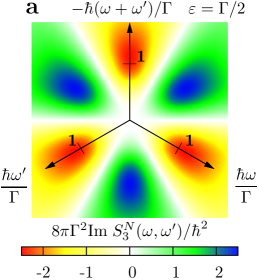
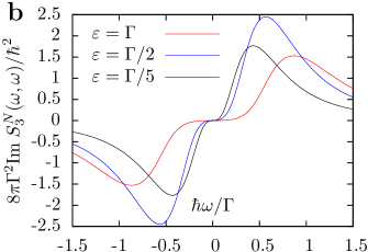
Figure 4: Time asymmetry of the third-order correlation of dot occupation fluctuations $S_{3}^{N}(\omega,\omega^{\prime})$ in frequency domain at $kT\ll\Gamma$. The symmetry is broken if $\mathrm{Im}\;S_{3}^{N}\neq 0$. (a) For $\varepsilon/\Gamma=0.5$ and arbitrary $\omega,\omega^{\prime}$ the asymmetry vanishes (white lines) at when $\omega$, $\omega^{\prime}$ or $\omega+\omega^{\prime}$ is equal to $0$. The hexagonal structure reflects the symmetry under permutations of frequencies. (b) Taking different values $\varepsilon/\Gamma=1,0.5,0.2$ and $\omega=\omega^{\prime}$ it is clear that the maximal asymmetry occurs for energy/frequency parameters of the same order.

For the experimental confirmation of the asymmetry one must introduce a weakly coupled detector. We propose an electric voltage-biased junction coupled weakly to the dot, so that its conductance depends on the charge on the dot, see figure 3(c). The externally measured quantity is the current $I$ through the junction, in particular $I\simeq I^{0}+\chi N$, where $I^{0}$ is the intrinsic current in the junction and $\chi$ is its susceptibility due to the dot’s charge. Then $S_{3}^{I}\simeq S_{3}^{I0}+\chi^{3}S_{3}^{N}$ where $S_{3}^{I0}$ is the internal current noise of the junction in the absence of the dot. Measurements of $S_{3}^{I0}$ have been demonstrated [25]; therefore we expect the measurement of $S_{3}^{I}$ to be feasible. Such an experiment will confirm the time-reversal symmetry violation only if the dot is not driven out of equilibrium. It is always possible for a certain parameter range—see Appendix B for the detailed model. Note that the dynamics of the detector here is clearly irreversible as it is initially in a nonequilibrium stationary state. However, we are only interested in the behavior of the system. Anyway, in the range of frequencies of possible asymmetry, $S^{I0}$ is frequency-independent, so the asymmetry of $S^{I}$ will show asymmetry of $S^{N}$.

6 Conclusions

We have shown that neither noninvasiveness (1) nor time symmetry (2) is automatically satisfied in the results of measurements, both classical and quantum. Only a subclass of detection schemes, parameterized by the measurement strength $g$, may satisfy (1) and/or (2). Classically, the measurement can be strictly noninvasive either at a finite $g$ and zero detector’s momentum or in the weak measurement limit, $g\to 0$. However, quantum noninvasiveness is satisfied only in a the limit of zero strength $g\to 0$. Moreover, the time symmetry of measurements (2) is broken in the quantum case, in contrast to classical mechanics. This is the fundamental difference between classical and quantum noninvasive measurements. One could argue that the weak measurement still affects the system and forces a time direction in this way. On the other hand, one expects a natural limit in which the influence on the system is negligible and the time symmetry should hold.

This violation is effectively a failure of weak measurements to accurately reflect the time-reversal symmetry inherent in a system. As such, it is independent of the validity of other symmetries such as charge parity time. Since quantum measurements of finite strength manifestly break time-reversal invariance, our result shows that, in contrast to classical measurements, all quantum measurements break time-reversal invariance regardless of their strength. Weak measurements are then still disturbing in some sense, although they do not disturb the state or later measurements.

Our result shows not only the quantum violation of time symmetry, but also the importance of a classical-quantum analogy of detection schemes. An open question is to what extent the analogy is correct. For instance, maybe not all system-detector interactions are allowed and possibly they cannot be instantaneous but rather time-extended. This needs further research, referring also to realistic experimental detection schemes.

Appendix A

To justify (6) we consider a series of weak measurements. Following Aharonov et al. [5], each weak measurement introduces an ancilla system and creates entanglement via an instant interaction Hamiltonian $\hat{H}_{I}=\hbar\delta(t)g\hat{p}\hat{A}$ where $g$ is the strength of interaction, $\hat{p}$ is momentum operator of the ancilla, conjugate to position $\hat{q}$ ($[\hat{q},\hat{p}]=i\hbar$), and $\hat{A}$ is the measured observable. The interaction is followed by von Neumann projection [2] of the ancilla onto a position eigenstate which destroys the ancilla. The system can however be measured again with the next ancilla, as shown in figure 1. The density matrix after the $j$^th measurement is

$$\hat{\rho}_{j}=\rme^{-\rmi g_{j}\hat{p}_{j}\hat{A}_{j}/\hbar}\left(\hat{\rho}_{j-1}\otimes|{\phi_{j}}\rangle\langle{\phi_{j}}|\right)\rme^{\rmi g_{j}\hat{p}_{j}\hat{A}_{j}/\hbar},$$ (A.1)

where $|{\phi_{j}}\rangle$ is the initial prepared state of ancilla $j$. By inserting identity operations $\int da\,|{a}\rangle\langle{a}|=\hat{1}$, the measurement interaction can be expressed as shifts of the ancilla wavefunction,

$$\hat{\rho}_{j}=\int\rmd a^{\prime}_{j}\,\rmd a^{\prime\prime}_{j}|{\phi_{j}(q_{j}-g_{j}a^{\prime}_{j})}\rangle\langle{\phi_{j}(q_{j}-g_{j}a^{\prime\prime}_{j})}||{a^{\prime}_{j}}\rangle\langle{a^{\prime}_{j}}|{\hat{\rho}}_{j-1}|{a^{\prime\prime}_{j}}\rangle\langle{a^{\prime\prime}_{j}}|.$$ (A.2)

In (A.2), the the state of ancilla $j$ which has the shifted wavefunction $\phi_{j}(x_{j}-g_{j}a^{\prime}_{j})$ is written as $|{\phi_{j}(x_{j}-g_{j}a^{\prime}_{j})}\rangle$. The joint probability $P(q_{1},\ldots,q_{n})=:P(\boldsymbol{q})$ is the probability of measuring the ancillas in a set of position eigenstates with positions given by $q_{k}$

$$P(\boldsymbol{q}) = \mathrm{Tr}\left\{\hat{\rho}_{n}\prod_{k}|{q_{k}}\rangle\langle{q_{k}}|\right\}$$

$$= \int\rmd\boldsymbol{a^{\prime}}\,\rmd\boldsymbol{a^{\prime\prime}}\,\delta(a^{\prime}_{n}-a^{\prime\prime}_{n})\tilde{\rho}_{n}\left(\boldsymbol{a^{\prime}},\boldsymbol{a^{\prime\prime}}\right)\prod_{k}\phi\left(q_{k}-g_{k}a^{\prime}_{k})\right)\phi^{\ast}\left(q_{k}-g_{k}a^{\prime\prime}_{k})\right).$$

In (Appendix A), $\tilde{\rho}_{j}$ is defined recursively by

$$\tilde{\rho}_{j}(a^{\prime}_{1},a^{\prime\prime}_{1},\ldots,a^{\prime}_{j},a^{\prime\prime}_{j})=\langle{a^{\prime}_{j}}|{a^{\prime}_{j-1}}\rangle\tilde{\rho}_{j-1}\langle{a^{\prime\prime}_{j-1}}|{a^{\prime\prime}_{j}}\rangle.$$ (A.4)

Using Gaussian wavefunctions $\phi(q)=(2\pi)^{-1/4}\,\rme^{-q^{2}/4}$, a change of variables to $\boldsymbol{\bar{a}}=(\boldsymbol{a^{\prime}}+\boldsymbol{a^{\prime\prime}})/2$ and $\boldsymbol{\delta a}=\boldsymbol{a^{\prime}}-\boldsymbol{a^{\prime\prime}}$ separates the joint probability density into a quasiprobability signal ($Q$) and detector noise ($D$).

$$P(\boldsymbol{q})=\int\rmd(\boldsymbol{\bar{a}})\;D(\boldsymbol{q}-\boldsymbol{g}\cdot\boldsymbol{\bar{a}})\,Q(\boldsymbol{\bar{a}}),$$

$$D(\boldsymbol{q}-\boldsymbol{g}\cdot\boldsymbol{\bar{a}})=\prod_{k}|\phi(q_{k}-g_{k}\bar{a}_{k})|^{2},$$ (A.5)

$$Q(\boldsymbol{\bar{a}})=\int\rmd\boldsymbol{\delta a}\;\rme^{-(\boldsymbol{g}\cdot\boldsymbol{\delta a})^{2}/2}\;\tilde{\rho}_{n}(\boldsymbol{\bar{a}},\boldsymbol{\delta a})\delta(\delta a_{n}).$$

Equation (A.5) defined the joint quasiprobability density $Q$ for the series of von Neumann measurements. The quasiprobability has a well-defined limit $g\to 0$. In this limit for time-resolved measurement, the averages with respect to this quasiprobability are given by

$$\langle a_{1}\cdots a_{n}\rangle=\int\rmd\boldsymbol{a}^{\prime}\rmd\boldsymbol{a}^{\prime\prime}\,\delta(a^{\prime}_{n}-a^{\prime\prime}_{n})\tilde{\rho}(\boldsymbol{a}^{\prime},\boldsymbol{a}^{\prime\prime})\prod_{k}\frac{a^{\prime}_{k}+a^{\prime\prime}_{k}}{2},$$ (A.6)

which is equivalent to (6). The genuine, measured probability $P=Q\ast D$ is positive definite because it contains also the large detection noise $\sim 1$ which is Gaussian, white and completely independent of the system, compared to the signal $\sim g$.

An alternative, equivalent approach is based on Gaussian positive operator-valued measures (POVMs) and special Kraus operators [3, 4, 26]. Let us begin with the basic properties of POVM. The Kraus operators $\hat{K}(a)$ for an observable described by $\hat{A}$ with continuous outcome $a$ need only satisfy $\int\rmd a\hat{K}^{\dagger}(a)\hat{K}(a)=\hat{1}$. The act of measurement on the state defined by the density matrix $\hat{\rho}$ results in the new state $\hat{\rho}(a)=\hat{K}(a)\hat{\rho}\hat{K}^{\dagger}(a)$. The new state yields a normalized and positive definite probability density $P(a)=\mathrm{Tr}\,\hat{\rho}(a)$. The procedure can be repeated recursively for an arbitrary sequence of (not necessarily commuting) operators $\hat{A}_{1},\dots,\hat{A}_{n}$,

$$\hat{\rho}(a_{1},\dots,a_{n})=\hat{K}(a_{n})\hat{\rho}(a_{1},\dots,a_{n-1})\hat{K}^{\dagger}(a_{n})\;.$$ (A.7)

The corresponding probability density is given by $P(a_{1},\dots,a_{n})=\mathrm{Tr}\;\hat{\rho}(a_{1},\dots,a_{n})$. We now define a family of Kraus operators, namely $\hat{K}_{g}(a)=(g^{2}/2\pi)^{1/4}\exp(-g^{2}(\hat{A}-a)^{2}/4)$. It is clear that $g\to\infty$ should correspond to exact, strong, projective measurement, while $g\to 0$ is a weak measurement and gives a large error. In fact, these Kraus operators are exactly those associated with the von Neumann measurements previously described. We also see that strong projection changes the state (by collapse), while $g\to 0$ gives $\hat{\rho}(a)\sim\hat{\rho}$, and hence this case corresponds to weak measurement. However, the repetition of the same measurement $k$ times effectively means one measurement with $g\to kg$ so, with $k\to\infty$, even a weak coupling $g\ll 1$ results in a strong measurement. For an arbitrary sequence of measurements, we can write the final density matrix as the convolution

$$\hat{\rho}_{\boldsymbol{g}}(\boldsymbol{a})=\int\rmd a^{\prime}\,\hat{\varrho}_{\boldsymbol{g}}(\boldsymbol{a}^{\prime})\prod_{k}d_{k}(a_{k}-a^{\prime}_{k})$$ (A.8)

with $d_{k}(a)=\rme^{-g^{2}a^{2}/2}\sqrt{g_{k}^{2}/2\pi}$. Here $\boldsymbol{g}=(g_{1},\dots,g_{n})$ $\boldsymbol{a}=(a_{1},\dots,a_{n})$, and $\rmd a=\rmd a_{1}\dots\rmd a_{n}$. The quasi-density matrix $\hat{\varrho}$ is given recursively by

$$\hat{\varrho}_{\boldsymbol{g}}(\boldsymbol{a}) = \int\frac{\rmd\xi}{2\pi}\rme^{-\rmi\xi a_{n}}\int\frac{\rmd\phi}{\sqrt{\pi g^{2}_{n}/2}}\rme^{-2\phi^{2}/g^{2}_{n}}$$

$$\times\rme^{\rmi(\xi/2+\phi)\hat{A}_{n}}\hat{\varrho}_{\boldsymbol{g}}(a_{1},\dots,a_{n-1})\rme^{\rmi(\xi/2-\phi)\hat{A}_{n}}$$

with the initial density matrix $\hat{\varrho}=\hat{\rho}$ for $n=0$. We can interpret $d$ in (A.8) as some internal noise of the detectors which, in the limit $g\to 0$, should not influence the system. We define the quasiprobability [6] $Q_{\boldsymbol{g}}=\mathrm{Tr}\,\hat{\varrho}_{\boldsymbol{g}}$ and abbreviate $Q\equiv Q_{\boldsymbol{0}}$. In this limit (Appendix A) reduces to

$$\hat{\varrho}(\boldsymbol{a})=\int\frac{\rmd\xi}{2\pi}\rme^{-\rmi\xi a_{n}}\rme^{\rmi\xi\hat{A}_{n}/2}\hat{\varrho}(a_{1},\dots,a_{n-1})\rme^{\rmi\xi\hat{A}_{n}/2}\,.$$ (A.10)

Note that $Q_{0\dots 0,g}=Q$, so the last measurement does not need to be weak (it can be even a projection). The averages with respect to $Q$ are easily calculated by means of the generating function (A.10), e.g. $\langle a\rangle_{Q}=\mathrm{Tr}\,\hat{A}\hat{\rho}$, $\langle ab\rangle_{Q}=\mathrm{Tr}\,\{\hat{A},\hat{B}\}\hat{\rho}/2$, $\langle abc\rangle_{Q}=\mathrm{Tr}\,\hat{C}\{\hat{B},\{\hat{A},\hat{\rho}\}\}/4$ for $\boldsymbol{a}=(a,b,c)$. As a straightforward generalization to continuous measurement, we obtain

$$\langle a_{1}(t_{1})\cdots a_{n}(t_{n})\rangle_{Q}=$$ (A.11)

$$\mathrm{Tr}\hat{\rho}\{\hat{A}_{1}(t_{1}),\{\cdots\{\hat{A}_{n-1}(t_{n-1}),\hat{A}_{n}(t_{n})\}\cdots\}\}/2^{n-1}$$

for time ordered observables, $t_{1}\leq t_{2}\leq\cdots\leq t_{n}$.

Appendix B

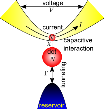
Figure 5: The model of detecting the dot’s charge. An electric junction contains another dot with effective occupation $N^{\prime}$, coupled capacitively to the measured dot. The fluctuations of the current $I$ in the junction biased by the voltage $V$ depend on the dot’s occupation $N$ with the proportionality constant $\chi$.

An effective model of weakly detecting the dot’s charge using an electric junction is shown in Fig. 5. The junction is treated as another dot between two reservoirs but in a broad level regime. The complete Hamiltonian, consisting of the dot part (5.2), and the junction part, reads

$$\hat{H}+\varepsilon^{\prime}\hat{N}^{\prime}+\hat{H}_{V}+e^{2}\hat{N}\hat{N}^{\prime}/C+eV\hat{Q}_{L}+\int\rmd E\;\times$$

$$\sum_{A=L,R}[\sqrt{\Gamma^{\prime}/2\pi}\hat{d}^{{\dagger}}\hat{\psi}_{A}(E)+\mbox{h.c.}+E\hat{\psi}_{A}(E)\hat{\psi}_{A}(E)],$$

$$\hat{N}_{L}=\hat{\psi}_{L}^{{\dagger}}(E)\hat{\psi}_{L}(E),\>\hat{N}^{\prime}=\hat{d}^{{\dagger}}\hat{d},$$ (B.1)

where $\hat{N}_{L}$ is the total number of elementary charges $e$ in the left reservoir, $C$ is the capacitance between the dot and the QPC, $\Gamma^{\prime}$,$\varepsilon^{\prime}$ denote effective tunneling rate and level energy of the QPC and $V$ is the bias voltage.

We measure current fluctuations in the junction, $I(t)$, with the current in Heisenberg picture defined as $\hat{I}(t)=-e\rmd\hat{N}_{L}(t)/\rmd t$. Such fluctuations have already been measured experimentally at low and high frequencies [25]. Most of fluctuations are just generated by the shot noise in the junction. Now, we consider a finite, but still very large capacitance. We expect a contribution from the system dot’s charge fluctuation to $S^{I}_{3}$ of the order $C^{-3}$. We assume separation of the system’s and detector’s characteristic frequency scales, namely

$$(\Gamma,\varepsilon,k_{B}T)\ll eV\ll(\Gamma^{\prime},\varepsilon^{\prime}),$$ (B.2)

which also includes the broad level approximation for the detector’s dot. There exists a special parameter range,

$$\frac{e^{2}}{\Gamma^{\prime}C}\gg\frac{\Gamma}{eV}\gg\left(\frac{e^{2}}{\Gamma^{\prime}C}\right)^{2},$$ (B.3)

where the coupling is strong enough to extract information about $N(t)$ which is not blurred by feedback and cross-correlation terms (left inequality), but weak enough not to drive the system dot out of equilibrium (right inequality). In this limit the dominating contributions to the detector current’s third cumulant are given by $S_{3}^{I}\simeq S_{3}^{I0}+\chi^{3}S_{3}^{N}$ with

$$S_{3}^{I0}=\mathcal{T}(1-\mathcal{T})(1-2\mathcal{T})e^{4}V/h,$$

$$\chi=-e^{2}\rmd\langle I\rangle/C\rmd\varepsilon^{\prime},$$ (B.4)

where $\langle I\rangle=\mathcal{T}e^{2}V/h$ and effective transmission $\mathcal{T}=\Gamma^{\prime 2}/(\varepsilon^{\prime 2}+\Gamma^{\prime 2})$. Although the $\sim\chi^{3}$ term in $S^{I}_{3}$ is much smaller than the first one, other terms, corresponding to cross correlations and back action, are negligible compared to the last term.

References

References

- [1] Leggett A J and Garg A 1985 Phys. Rev. Lett. 54 857
- [2] von Neumann J 1932 Mathematical Foundations of Quantum Mechanics (Princeton: Princeton U.P.)
- [3] Wiseman H M and Milburn G J 2009 Quantum Measurement and Control (Cambridge: Cambridge University Press)
- [4] Kraus K 1983 States, Effects and Operations (Berlin: Springer)
- [5] Aharonov Y, Albert D Z and Vaidman L 1988 Phys. Rev. Lett. 60 1351
- [6] Bednorz A and Belzig W 2010 Phys. Rev. Lett. 105 106803 Bednorz A, Belzig W and Nitzan A 2012 New J. Phys. 14 013009
- [7] Lundeen J S, Sutherland B, Patel A, Stewart C and Bamber C 2011 Nature 474 188
- [8] Ruskov R, Korotkov A N and Mizel A 2006 Phys. Rev. Lett. 96 200404
- [9] Jordan A N, Korotkov A N and Büttiker M 2006 Phys. Rev. Lett. 97 026805
- [10] Williams N S and Jordan A N 2008 Phys. Rev. Lett. 100 026804
- [11] Palacios-Laloy A, Mallet F, Nguyen F, Bertet P, Vion D, Esteve D and Korotkov A N 2010 Nat. Phys. 6 442
- [12] Streater R F and Wightman A S 1964 PCT, spin and statistics, and all that (New York: Benjamin)
- [13] Sozzi M 2008 Discrete Symmetries and CP Violation (New York: Oxford U.P.)
- [14] Greenberg O W 2002 Phys. Rev. Lett. 89 231602
- [15] van Kampen N G 2007 Stochastic Processes in Physics and Chemistry, (Amsterdam: North-Holland)
- [16] Onsager L 1931 Phys. Rev. 37 405
- [17] Aharonov Y, Bergmann P G and Lebowitz J L 1964 Phys. Rev. 134 B1410 Gell-Mann M and Hartle J 1994 Physical Origins of Time Asymmetry eds. Halliwell J, Perez-Mercader J and Zurek W (Cambridge: Cambridge University Press) 311 (Preprint arXiv:gr-qc/9304023)
- [18] Aharonov Y, Popescu S and Tollaksen J 2010 Phys. Today 63 i.11 27
- [19] Berg B, Plimak L I, Polkovnikov A, Olsen M K, Fleischhauer M and Schleich W P 2009 Phys. Rev. A 80 033624 Tsang M 2009 Phys. Rev. A 80 033840 Hofmann H F 2010 Phys. Rev. A 81 012103 Dressel J, Agarwal S, and Jordan A N 2010 Phys. Rev. Lett. 104 240401 Chou K, Su Z, Hao B and Yu L 1985 Phys. Rep. 118 1
- [20] Dirac P A M 1958 The principles of Quantum Mechanics (New York: Oxford U.P.)
- [21] Lu W, Ji Z, Pfeiffer L, K. W. West K W and Rimberg A J 2003 Nature 423422 Sukhorukov E V, Jordan A N, Gustavsson S, Leturcq R, Ihn T and Ensslin K 2007 Nature Phys. 3 243
- [22] Blanter Y M and Büttiker M 2000 Phys. Rep. 336 1
- [23] Schwinger J 1961 J. Math. Phys. 2 407 Keldysh L V 1965 Sov. Phys – JETP 20 1018 Kadanoff L P, Baym G 1962 Quantum Statistical Mechanics (New York: Benjamin) Kamenev A and Levchenko A 2009 Advances in Phys. 58 197
- [24] Utsumi Y 2007 Phys. Rev. B 75 035333
- [25] Reulet B, Senzier J, and Prober D E 2003 Phys. Rev. Lett. 91 196601 Bomze Y, Gershon G, Shovkun D, Levitov L S and Reznikov M 2005 Phys. Rev. Lett. 95 176601 Gershon G, Bomze Y, Sukhorukov E V and Reznikov M 2008 Phys. Rev. Lett. 101 016803 Gabelli J and Reulet B 2009 J. Stat. Mech. P01049 doi:10.1088/1742-5468/2009/01/P01049
- [26] Barchielli A, Lanz L and Prosperi G M 1982 Nuovo Cimento B 72 79 (1982) Caves C M and Milburn G J 1987 Phys. Rev. A 36 5543 (1987) Schmid A 1987 Ann. Phys. 173 103