Neutrino masses beyond the tree level

Abstract

Models for Majorana neutrino masses can be classified according to the level in perturbation theory at which the effective dimension five operator $LLHH$ is realized. The possibilities range from the tree-level up to the three-loop level realizations. We discuss some general aspects of this approach and speculate about a model independent classification of the possible cases. Among all the realizations, those in which the effective operator is induced by radiative corrections open the possibility for lepton number violation near -or at- the electroweak scale. We discuss some phenomenological aspects of two generic radiative realizations: the Babu-Zee model and supersymmetric models with bilinear R-parity violation.

1 Introduction

Neutrino experiments have firmly demonstrated neutrinos are massive and have non-vanishing mixing angles among the different generations Schwetz:2008er . Since in the standard model neutrinos are massless this experimental results are a clear evidence of beyond standard model physics. From a general point of view Majorana neutrino masses can be generated by adding to the standard model Lagrangian the non-renormalizable effective Lagrangian Weinberg:1980bf

$${\cal L}_{5}\sim\frac{1}{\Lambda_{\text{NP}}}{\cal O}_{5}=\frac{1}{\Lambda_{\text{NP}}}\left(\overline{L^{c}}i\tau_{2}H\right)\;\left(Hi\tau_{2}L\right)\,,$$ (1)

where $L$ and $H$ are the lepton and Higgs electroweak doublets. The presence of the effective Lagrangian in (1) guarantees that after electroweak symmetry breaking neutrinos acquire Majorana masses. Extensions of the standard model in which neutrinos have Majorana masses realize the effective operator ${\cal O}_{5}$ in different ways. However, among all these possibilities there are subsets that have a common feature, namely the order in perturbation theory at which the operator is realized. As will be discussed in sec. 2 a rather general classification of neutrino mass models can be done by gathering together these different subsets.

Making an exhaustive list of possible realizations of ${\cal O}_{5}$ and their corresponding phenomenology is far out of the scope of the present discussion. Thus, instead of using this approach we will discuss two classes of generic models: models in which neutrino masses are generated radiatively at the 2-loop level and supersymmetric models with broken R-parity. In the former case we will stick to the Babu-Zee model Zee:1985id ; Babu:1988ki , while for the latter we will discuss bilinear R-parity breaking models with a neutralino LSP Porod:2000hv .

2 The ${\cal O}_{5}$ operator and its different realizations

At $\Lambda_{\text{NP}}$ the heavy physical degrees of freedom, that when integrated out yield the dimension five ($d=5$) effective operator ${\cal O}_{5}$, are no longer decoupled. Once specified they define a particular model for Majorana neutrino mass generation, so different models lead to different realizations of ${\cal O}_{5}$. As pointed out in the introduction these realizations can be classified according to the order in perturbation theory at which ${\cal O}_{5}$ is generated, namely tree-level (${\cal O}_{5}^{\ell=0}$), one-loop (${\cal O}_{5}^{\ell=1}$), two-loops (${\cal O}_{5}^{\ell=2}$) and three-loops (${\cal O}_{5}^{\ell=3}$), where $\ell$ denotes the number of loops in each case. Three-loop level realizations require order one Yukawa couplings implying that models based on ${\cal O}_{5}^{\ell\geq 4}$ are, in general, not consistent with neutrino data once the requirement of perturbativity of the corresponding couplings is imposed.

A general and model independent classification of the tree-level ${\cal O}_{5}^{\ell=0}$ and one-loop level ${\cal O}_{5}^{\ell=1}$ realizations of ${\cal O}_{5}$ has been carried out in ref. Ma:1998dn and such an analysis could be, in principle, extended to the two and three loop order realizations. Regardless of the order at which the operator arises the procedure is based on the determination of all the possible gauge invariant renormalizable vertices within the loop for all the different possible topologies. In this procedure the only gauge quantum numbers that are fixed are those of the external legs ($LLHH$) while those of the physical degrees of freedom flowing in the loop are free and should be fixed by the requirement of gauge invariance. Another approach for the same sort of classification is by using all the possible $\Delta L=2$ effective operators up to certain $d$. This method has been implemented in ref. Babu:2001ex for effective operators up to $d=11$. The difference between these two approaches is that while the former focus exclusively on the ${\cal O}_{5}$ operator the later covers this operator but also higher dimensional operators as e.g. ${\cal O}_{7}\sim(LLHH)(H^{\dagger}H)$. Note that these higher dimensional effective operators ($d>5$) can give a dominant contribution to neutrino masses only if the leading effective operator ${\cal O}_{5}$ is forbiden due to a new symmetry. These cases have been throughout analysed in ref. Bonnet:2009ej and we have nothing more to add here.

The tree-level realizations of ${\cal O}_{5}$ correspond to the different type of seesaw models (type-I seesaw , type-II Schechter:1980gr and type-III Foot:1988aq ) whereas for the 1-loop cases the number of possibilities (models) is much more larger (is determined by the different $SU(3)\times SU(2)\times U(1)$ assignments of the internal degrees of freedom flowing in the loop). Examples of ${\cal O}_{5}^{\ell=1}$ include the Zee model Zee:1980ai , models with scalar leptoquarks AristizabalSierra:2007nf and models with extra scalars and fermions with nontrivial color charges FileviezPerez:2009ud . Examples of two-loop realizations include extended scalar sectors as in the case of the the Babu-Zee model Zee:1985id ; Babu:1988ki and models with scalar leptoquarks Babu:2001ex ; Babu:2010vp . Up to our knowledge three-loop level realizations rely on extensions of both the scalar and fermion sectors, examples can be found in references Babu:2001ex ; Krauss:2002px .

In models in which the operator ${\cal O}_{5}$ is generated beyond the tree-level the lepton number breaking scale can readily be at or around the electroweak scale. Thus, models embedded in such realizations usually lead to testable predictions in either high-energy or high-intensity experiments. In what follows we will discuss two main cases, the Babu-Zee model and supersymmetric bilinear R-parity violating models, paying special attention to some of their phenomenological implications.

3 Two loop realization: the Babu-Zee model

In this model the standard model scalar sector is extended by the addition of two new scalars, $h^{+}$ and $k^{++}$, both singlets under $SU(2)$. Their couplings to standard model leptons is given by

$${\cal L}=f_{\alpha\beta}(L^{Ti}_{\alpha L}CL^{j}_{\beta L})\epsilon_{ij}h^{+}+h^{\prime}_{\alpha\beta}(e^{T}_{\alpha R}Ce_{\beta R})k^{++}+{\rm h.c.}$$ (2)

Here, $L_{L}$ are the standard model (left-handed) lepton doublets, $e_{R}$ the charged lepton singlets, $\alpha,\beta$ are generation indices and $\epsilon_{ij}$ is the completely antisymmetric tensor. Note that $f$ is antisymmetric, while $h^{\prime}$ is symmetric. Assigning $L=2$ to $h^{-}$ and $k^{++}$, eq. (2) conserves lepton number. Lepton number violation in the model resides only in the following term in the scalar potential

$${\cal L}=-\mu h^{+}h^{+}k^{--}+{\rm h.c.}$$ (3)

Here, $\mu$ is a parameter with dimension of mass.

The setup of eq. (2) and eq. (3) generates Majorana neutrino masses via the two-loop diagram shown in fig. (1). The resulting neutrino mass matrix can be expressed as

$${\cal M}^{\nu}_{\alpha\beta}=\frac{8\mu}{(16\pi^{2})^{2}m_{h}^{2}}f_{\alpha x}\omega_{xy}f_{y\beta}{\cal I}(\frac{m_{k}^{2}}{m_{h}^{2}}),$$ (4)

with summation over $x,y$ implied. The parameters $\omega_{xy}$ are defined as $\omega_{xy}=m_{x}h_{xy}m_{y}$, with $m_{x}$ the mass of the charged lepton $l_{x}$. Following Babu:2002uu we have rewritten $h_{\alpha\alpha}=h^{\prime}_{\alpha\alpha}$ and $h_{\alpha\beta}=2h^{\prime}_{\alpha\beta}$. ${\cal I}(r)$ finally is a dimensionless two-loop integral given by

$${\cal I}(r)=-\int_{0}^{1}dx\int_{0}^{1-x}dy\frac{1}{x+(r-1)y+y^{2}}\log\frac{y(1-y)}{x+ry}.$$ (5)

For non-zero values of $r$, ${\cal I}(r)$ can be solved only numerically. We note that for the range of interest, say $10^{-2}\leq r\leq 10^{2}$, ${\cal I}(r)$ varies quite smoothly between (roughly) $3\leq{\cal I}(r)\leq 0.2$.

Figure 1: Feynman diagram for the 2-loop Majorana neutrino masses in the model of Zee:1985id ; Babu:1988ki .

3.1 Flavour violating charged lepton decays

Phenomenological tests of this model have been studied in Babu:2002uu ; AristizabalSierra:2006gb ; Nebot:2007bc . Among all of them those involving $\mu\to e\gamma$ can be regarded as the most stringent ones. In ref. AristizabalSierra:2006gb it has been shown that the corresponding decay branching ratio for this process can be written as

$$Br(\mu\rightarrow e\gamma) \simeq 4.5\cdot 10^{-10}\Big{(}\frac{\epsilon^{2}}{h_{\mu\mu}^{2}{\cal I}(r)^{2}}\Big{)}\Big{(}\frac{m_{\nu}}{\rm 0.05\hskip 2.84526pteV}\Big{)}^{2}\Big{(}\frac{\rm 100\hskip 2.84526ptGeV}{m_{h}}\Big{)}^{2}\,,$$ (6)

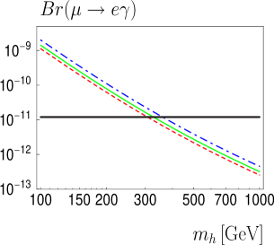
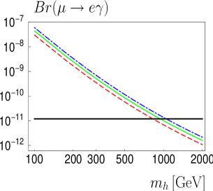
with $\epsilon=f_{e\tau}/f_{\mu\tau}$ and $m_{h}$ the mass of the singly charged scalar. Figure 2 shows the resulting lower limit on $Br(\mu\to e\gamma$) as a function of $m_{h}$ for the case of normal and inverted hierarchies. Note that the horizontal solid line indicates the upper limit set by the MEGA experiment Brooks:1999pu and not the new one placed by the MEG experiment, $Br(\mu\to e\gamma)<2.4\times 10^{-12}$ at 90% C.L. Adam:2011ch . Using the updated limits the constraints on the singly charged scalar mass would be even more stringent that the ones quoted here.

In summary, in this model $Br(\mu\to e\gamma)\geq 10^{-13}$ is guaranteed for singly charged scalar masses smaller than 590 GeV (5.04 TeV) for normal (inverse) hierarchical neutrino masses, and larger or even much larger branching ratios are expected in general. Thus, a non-observation of this process in the next few years, at least for the case of inverse hierarchy, would certainly remove most of the motivation to study this model.

Figure 2: Conservative lower limit on the branching ratio Br($\mu\rightarrow e\gamma$) as a function of the charged scalar mass $m_{h}$ for normal hierarchy (left plot) and inverted hierarachy (right plot). The three lines are for the current solar angle $\sin^{2}\theta_{12}$ best fit value (full line) and 3 $\sigma$ lower (dashed line) and upper (dot-dashed line) bounds. Other parameters fixed at $\sin^{2}\theta_{23}=0.5$, $\sin^{2}\theta_{13}=0.040$ and $\Delta m^{2}_{\rm Atm}=2.0\cdot 10^{-3}$ eV².

4 Bilinear R-parity violating supersymmetry

Bilinear R-parity violation (BRpV) provides an intrinsically supersymmetric framework for Majorana neutrino masses (for a review see Hirsch:2004he ). In these models the superpotential includes, in addition to the MSSM terms, also the term

$$W_{\text{BRpV}}=\epsilon_{i}\hat{L}_{i}\hat{H}_{u}\,.$$ (7)

This term breaks not only R-parity but also lepton number in all three generations. In order to have a consistent model a soft SUSY breaking term has to be added to the scalar potential, namely

$$V_{\text{BRpV}}^{\text{soft}}=B_{i}\epsilon_{i}\tilde{L}_{i}H_{u}\,.$$ (8)

The presence of these terms induce a non-vanishing vacuum expectation value for the sneutrinos ($v_{i}=\langle\tilde{\nu}_{i}\rangle$) that give rise to a mixing among neutral gauginos and Higgsinos with neutrinos. Due to this mixing one of the neutrinos acquires mass. The effective neutrino mass matrix reads

$$(m_{\nu}^{(0)})_{ij}=\frac{M_{1}g^{2}+M_{2}g^{\prime 2}}{4\text{det}\,(\boldsymbol{M_{\chi^{0}}})}\;\Lambda_{i}\Lambda_{j}\,,$$ (9)

where $\Lambda_{i}=\mu v_{i}+v_{d}\epsilon$ (with $\mu$ the Higgsino mass term and $v_{d}=\langle H_{d}\rangle$) and $\boldsymbol{M_{\chi^{0}}}$ is the neutralino mass matrix. The other two neutrinos acquire mass from one-loop corrections involving $W$, $Z$ and scalar loops, being the bottom-sbottom and tau-stau loops the most important contributions Hirsch:2000ef . Thus, the BRpV model is an example of a model in which neutrino masses arise from different realizations of the ${\cal O}_{5}$ operator.

The atmospheric and reactor angles are approximately given by the rotation angles that diagonalize the tree level mass matrix $m_{\nu}^{(0)}$:

$$\tan^{2}\theta_{23}\approx\frac{\Lambda_{2}^{2}}{\Lambda_{3}^{2}},\quad\tan^{2}\theta_{13}\approx\frac{\Lambda_{1}^{2}}{\Lambda_{3}^{2}+\Lambda_{2}^{2}}\,.$$ (10)

The solar angle instead is obtained once the one-loop corrections are taken into account. A remarkable feature of the bilinear R-parity breaking model is that the same parameters that determine neutrino physics also control the decay patterns of the LSP, thus it is always possible to establish a set of correlations between the LSP decay branching ratios and neutrino observables. These correlations can be used as a tool to know whether BRpV is responsible for the origin of neutrino masses.

4.1 LSP decays and neutrino observables

Once R-parity is broken the LSP is unstable and decays to standard model fermions. Thus astrophysical contraints on its nature do not hold any more and in principle any supersymmetric particle can be the LSP. The decay patterns of all possible LSPs and their relations with neutrino observables in the context of bilinear R-parity breaking models have been analysed in Porod:2000hv ; Hirsch:2003fe . Additional studies in more generic models including trilinear R-parity violating couplings have been carried out for slepton and sneutrino LSPs Bartl:2003uq ; Aristizabal Sierra:2004cy . Here we will highlight some of the main features of this “program” in bilinear R-parity breaking models assuming the lightest neutralino to be the LSP. The following discussion is based on ref. Porod:2000hv .

The presence of the bilinear R-parity violating parameters induce not only a mixing between neutralinos and neutrinos but also a mixing between charginos and charged leptons, charged Higgses and sleptons, CP-even (CP-odd) components of the neutral Higgses and the corresponding CP-even (CP-odd) components of the sneutrinos Hirsch:2000ef . All together these mixings determine the three-body leptonic, semi-leptonic and invisible neutralino decays: $\tilde{\chi}^{0}_{1}\to\nu_{i}l_{j}^{+}l_{k}^{-}$, $\tilde{\chi}^{0}_{1}\to l^{\pm}_{i}q\bar{q}^{\prime}$, $\tilde{\chi}^{0}_{1}\to\nu_{i}q\bar{q}$ and $\tilde{\chi}^{0}_{1}\to\nu_{i}\nu_{j}\nu_{k}$.

Figure 3: Ratios of decay branching ratios for semi-leptonic neutralino decays and their correlations with the atmospheric and reactor angles Porod:2000hv .

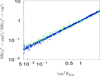
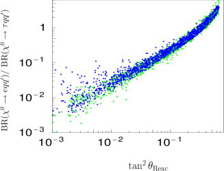
Given the above discussion it should now become clear that once the bilinear R-parity breaking parameters are constrained by neutrino experimental data the lightetest neutralino decays are expected to be constrained as well. In fact, it turns out that the constraints imposed by neutrino physics assure: ($i$) the neutralino always decay inside the detector; ($ii$) the decay branching ratio for neutralino invisible decays never exceeds 10%; ($iii$) different ratios of decay branching ratios are strongly correlated with neutrino mixing angles. Figure 3 shows the corresponding correlations for the semi-leptonic final states $\mu qq^{\prime}$, $\tau qq^{\prime}$ and $eqq^{\prime}$. From these results and the measured neutrino mixing angles it can be established that if BRpV is the mechanism responsible for the origin of neutrino masses and the lightest neutralino turn out the be the LSP the following measurements should be expected at LHC:

$$\text{BR}(\tilde{\chi}^{0}_{1}\to\mu qq^{\prime})\simeq\text{BR}(\tilde{\chi}^{0}_{1}\to\tau qq^{\prime})\quad\text{and}\quad\text{BR}(\tilde{\chi}^{0}_{1}\to eqq^{\prime})\ll\text{BR}(\tilde{\chi}^{0}_{1}\to\mu qq^{\prime})\,.$$ (11)

In summary, in bilinear R-parity breaking models the decay patterns of the LSP are strongly correlated with neutrino mixing angles. These correlations allow to set constraints on the different decay branching ratios of the LSP that in turn can be used to prove whether these models are responsible for the origin of neutrino masses and mixings.

5 Conclusions

From a general perspective Majorana neutrino masses can be accounted for by the effective dimension five operator ${\cal O}_{5}$. We have argued that the different “incarnations” of this operator can be classified according to the order in perturbation theory at which the operator is realized. In principle by using group theoretical arguments one could make, in a model independent way, an exhaustive list of all the possibilities at each order and up to the three-loop level .

Models in which ${\cal O}_{5}$ is realized radiatively (${\cal O}_{5}^{\ell\neq 0}$, where $\ell$ denotes the numer of loops) rely on TeV scale physics. Thus, an obvious question is whether this new physics, and therefore the origin of neutrino masses, can be proved at e.g. the LHC. As illustrative examples we have discussed what we consider two benchmark models: The Babu-Zee model and supersymmetry with bilinear broken R-parity.