Tree method for quantum vortex dynamics

Abstract

We present a numerical method to compute the evolution of vortex filaments in superfluid helium. The method is based on a tree algorithm which considerably speeds up the calculation of Biot-Savart integrals. We show that the computational cost scales as $N\log{(N)}$ rather than $N^{2}$, where $N$ is the number of discretization points. We test the method and its properties for a variety of vortex configurations, ranging from simple vortex rings to a counterflow vortex tangle, and compare results against the Local Induction Approximation and the exact Biot-Savart law.

I Introduction

Quantum turbulence Donnelly ; Barenghi-Sergeev ; Halperin consists of a disordered tangle of reconnecting quantized vortex filaments, each carrying one quantum of circulation $\kappa$. This form of turbulence is easily created by agitating superfluid liquid helium (⁴He) with propellers Tabeling ; Roche2007 , forksSkrbek , or grids Smith1993 , the same techniques which are used to create turbulence in ordinary fluids. There are also methods which are unique to superfluid liquid helium, for example heat flows Vinen1957 ; Paoletti2008 and streams of ions Walmsley2008 . Quantum turbulence is also studied in superfluid ³He-B Eltsov2010 ; Lancaster2011 and, more recently, in atomic Bose-Einstein condensatesHenn2009 . In the study of quantum turbulence, particular attention is devoted to the similarities with ordinary turbulence Vinen-Niemela ; Lvov-Nazarenko . Recent progress has been boosted by the development of new flow visualization techniques, such as tracer particlesMaryland-tracers ; VanSciver , Andreev scattering Lancaster-Andreev and laser-induced fluorescenceYale .

This article is concerned with numerical simulations of quantum turbulence. Starting from the pioneering work of Schwarz Schwarz , numerical simulations have always played an important role in the field Samuels ; Aarts ; Bauer ; Tsubota2003 ; Risto ; Konda ; Kivo ; Morris ; Kivo2 ; cascade ; tree . The recent experimental progress, rather than reducing the need of numerical simulations, has highlighted their importance in interpreting visualization methods Kivotides-PIV ; Finne .

In superfluid ⁴He, the vortex core radius ($a_{0}\approx 10^{-8}~{}\rm cm$) is many orders of magnitude smaller than the average separation between vortex lines (typically from $10^{-2}$ to $10^{-4}\rm cm$) or any other relevant length scale in the flow. This feature was early recognised by SchwarzSchwarz , who proposed to model vortex lines as spaces curves $\mathbf{s}=\mathbf{s}(\xi,t)$ of infinitesimal thickness, where $t$ is the time and $\xi$ is arc length. This vortex filament approach is also valid in ³He-B, although to a lesser extent because the core size is larger ($a_{0}\approx 10^{-6}~{}\rm cm$). The space curves are numerically discretized by a large, variable number of points $\mathbf{s}_{i}$ ($i=1,\cdots N)$, which hereafter we refer to as vortex points.

At temperatures low enough that the normal fluid and mutual friction is negligible, the governing equation of motion of the superfluid vortex lines is the Biot-Savart (BS) law Saffman

$$\frac{d\mathbf{s}}{dt}=-\frac{\kappa}{4\pi}\oint_{\cal L}\frac{(\mathbf{s}-\mathbf{r})}{|\mathbf{s}-\mathbf{r}|^{3}}\times{\bf d}\mathbf{r},$$ (1)

where the line integral extends over the entire vortex configuration $\cal L$. Eq. (1) formulates the classical Euler dynamics of vortex filaments in incompressible inviscid flows. The assumption of incompressibility is justified, as all relevant speeds, of the order of few cm/s, are much smaller than the speed of sound, which is approximately $240~{}\rm m/s$ (but see the discussion of reconnections and dissipation in Section III). Unlike vortex lines in classical inviscid Euler flows, however, superfluid vortex lines can reconnect with each other when they come sufficiently close Koplik ; Bewley ; Tebbs ; Kerr ; Bajer . This effect is captured by a more microscopic model, the Gross-Pitaevskii Equation (GPE) for a Bose-Einstein condensateinfinite . In the context of the vortex filament approach, reconnections are modelled by supplementing Eq. (1) with an algorithmical reconnection procedure, as originally proposed by Schwarz Schwarz .

Two difficulties arise in seeking a numerical solution of Eq. (1). Firstly Eq. (1) is singular at $\mathbf{s}=\mathbf{r}$. Following Schwarz Schwarz , to circumvent this problem we split the velocity of the filament of the $i^{\textrm{th}}$ vortex point $\mathbf{s}_{i}$ into a local contribution (near the singularity) and non-local contributions, writing

$$\frac{d\mathbf{s}_{i}}{dt}=\frac{\kappa}{4\pi}\ln\left(\frac{\sqrt{\ell_{i}\ell_{i+1}}}{a_{1}}\right)\mathbf{s}_{i}^{\prime}\times\mathbf{s}_{i}^{\prime\prime}-\frac{\kappa}{4\pi}\oint_{\cal L^{\prime}}\frac{(\mathbf{s}_{i}-\mathbf{r})}{|\mathbf{s}_{i}-\mathbf{r}|^{3}}\times{\bf d}\mathbf{r}.$$ (2)

Here a prime denotes a derivative with respect to arc length (hence $\mathbf{s}^{\prime}=d\mathbf{s}/d\xi$ and $\mathbf{s}^{\prime\prime}=d^{2}\mathbf{s}/d\xi^{2}$), $\ell_{i}$ and $\ell_{i+1}$ are the arclengths of the curves between points $\mathbf{s}_{i-1}$ and $\mathbf{s}_{i}$ and between $\mathbf{s}_{i}$ and $\mathbf{s}_{i+1}$, $\cal L^{\prime}$ is the original vortex configuration $\cal L$ without the section between $\mathbf{s}_{i-1}$ and $\mathbf{s}_{i+1}$, and $a_{1}$ is a cutoff parameter. For simplicity, hereafter we assume that the cutoff parameter is equal to the vortex core radius, $a_{1}\approx a_{0}$.

To numerically calculate the nonlocal term in Eq. (2), we must perform further manipulations. We follow Schwarz and split the integral into discrete parts, which account for the contribution of the vortex between points along $\cal L^{\prime}$. Assuming a straight line between vortex points, the contribution to the nonlocal term due to the vortex segment between points $\mathbf{s}_{j}$ and $\mathbf{s}_{j+1}$ is given by,

$$\Delta v_{nl}^{j}(\mathbf{s}_{i})=\frac{\kappa}{2\pi(4AC-B^{2})}\left[\frac{2C+B}{\sqrt{A+B+C}}-\frac{B}{\sqrt{A}}\right]\mathbf{p}\times\mathbf{q}.$$ (3)

Where $\mathbf{p}=\mathbf{s}_{j}-\mathbf{s}_{i}$, $\mathbf{q}=\mathbf{s}_{j+1}-\mathbf{s}_{j}$, $A=|\mathbf{p}|^{2}$, $B=2\mathbf{p}\cdot\mathbf{q}$ and $C=|\mathbf{q}|^{2}$. The total nonlocal contribution is then found by summing over all $j\in\cal L^{\prime}$.

The second difficulty, which we address in this paper, is the computational cost of the BS law. It is apparent from Eq. (1) that the velocity at one vortex point depends on an integral over all other $N-1$ points, so the CPU time required to evolve the vortex configuration in time scales as $N(N-1)\sim N^{2}$. Because of this cost, it has been difficult to numerically calculate vortex tangles with vortex line density $L$ (vortex length per unit volume) comparable to what is achieved in experiments. Similarly, it has been difficult to perform sufficiently long numerical calculations which are needed, for example, to saturate the initial vortex configuration to a steady state tangle, or to produce long time series suitable for spectral analysis, or to study the decay of quantum turbulence.

Schwarz Schwarz proposed the Local Induction Approximation (LIA) DaRios ; Arms-Hama as a practical alternative to the exact (but CPU-intensive) BS law. Neglecting the second non-local term in Eq. (2), we have simply

$$\frac{d\mathbf{s}_{i}}{dt}=\frac{\kappa}{4\pi}\ln\biggl{(}\frac{c\langle R\rangle}{a_{0}}\biggr{)}\mathbf{s}_{i}^{\prime}\times\mathbf{s}_{i}^{\prime\prime},$$ (4)

where $c$ is a constant of order unity and $\langle R\rangle$ is the mean radius of curvature of the vortex filament. The LIA greatly increases the efficiency of the numerical code because its computational cost scales with $N$, as opposed to $N^{2}$ for the BS law. Moreover the LIA offers insight into vortex dynamics. Using LIA, it is easy to show that, in the first approximation, the motion of a point on the vortex filament is along the direction which is binormal to the filament at that point, with speed which is inversely proportional to the local radius of curvature $R=1/|\mathbf{s}^{\prime\prime}|$. Moreover the LIA describes well the translational motion of a circular vortex ring and the rotation of a small amplitude Kelvin wave.

Unfortunately, the LIA does not capture the interaction between two vortex filaments, and the interaction which different parts of the same vortex have on each other. For example, two circular vortex rings, set coaxially close to each other, move in a leapfrogging fashion, but the effect is ignored by the LIA. Other limitations of the LIA have been discussed in the literature Ricca ; Boffetta2009 ; Adachi2010 . Clearly the LIA is not the best tool to study important properties of turbulence which arise from the vortex interaction, such as how the energy is distributed over the length scales (the Kolmogorov spectrum).

In a recent paper tree we presented the spectrum of vortex density fluctuations in superfluid turbulence and compared it to experiments. This calculation was possible because we used a tree algorithm, which retains the long-range interaction of the BS law, but sensibly approximate it, so that its computational cost scaled as $N\log{(N)}$ rather than $N^{2}$. The difference between $N^{2}$ and $N\log{(N)}$ cannot be overstated: it is the same improvement of the Fast Fourier Transform. For example, in the work reported in ref. tree , the typical number of vortex points which we used was of the order of $N\sim 10^{5}$. Tree algorithms are popular in astrophysical N-body simulations Springel2010 . The numerical solution of the gravitational interaction of $N$ bodies, in fact, has the same difficulty of the BS law: the motion of one body depends on the other $N-1$ bodies, hence the computational cost scales as $N^{2}$, as for vortex points.

The aim of this paper is to present a detailed description of a tree algorithm tailored to vortex dynamics, provide quantitative error estimates associated with the method, and compare results with methods used in the literature. In particular we show that the tree method provides huge computational savings but without the inherent errors associated with the LIA.

The structure of the article is as follows. Section II outlines the algorithms and methods required to create a tree structure for a set of points embedded in three-dimensional space. We pay careful attention to how this tree structure can be efficiently used to compute the velocity at a particular vortex point. In Section III we provide further details on the algorithms required to apply the vortex filament method to the study of quantised turbulence. Section IV contains the results of numerical tests of the tree algorithm. We show that the $N^{2}$ scaling inherent in the evaluation of the BS integral can be approximated, with a tolerable loss of accuracy, by a tree method which exhibits an improved $N\log N$ scaling. A recent, and very detailed, numerical study of counterflow turbulence by Adachi et al. Adachi2010 as again demonstrated that the LIA is unsuitable for the study of quantum turbulence. In Section V we verify that the tree method does not exhibit the same deficiencies of the LIA.

In all simulations presented, here we use parameters which refer to superfluid ⁴He: circulation $\kappa=9.97\times 10^{-4}~{}\rm cm^{2}/s$ and vortex core radius $a_{0}\approx 10^{-8}~{}\rm cm$. All our results and methods, however, can be generalised to vortex systems in low temperature ³He-B.

II Tree algorithm

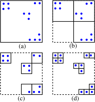
Figure 1: (Color online) Illustration of the tree construction in two dimensions (quad-tree). The points (blue dots) are enclosed in the root cell (a), which is divided into four cells of half size (b), until (c,d) there is only one point per cell.

Building on the pioneering work of Barnes and Hut Barnes1986 , the majority of astrophysical and cosmological N-body simulations have made use of tree algorithms to enhance the efficiency of the simulation with a relatively small loss in accuracy Bertschinger1998 . The advantages of these methods are two-fold. Firstly they have been shown to scale as $N\log(N))$, where $N$ is the number of particles used in the simulation. Secondly there are now openly available parallel implementations of the tree algorithm, which have been used to compute simulations with up to 10 billion particles Springel2005 . Our implementation of the tree algorithm for vortex dynamics is limited to a serial program, however the development of a parallel scheme is one of our future aims.

We are not the first to apply tree methods to quantised vortex simulations. Kivotedes Kivotides2007 used a tree method to enhance a vortex filament simulation, but did not provide any description, testing and evaluation of the performance of the method. Kozik and Svistunov Kozik2005 introduced an interesting method to speed up the simulation of the Kelvin wave cascade along quantised vortices using a scale separation scheme. Whilst this is a significant improvement over the full BS integral the problem discussed in Kozik2005 is inherently one-dimensional and it is not clear if there is an efficient implementation of the scheme that would enhance the speed of a three dimensional simulation.

Detailed descriptions of the tree algorithm can be found in a number of works Salmon1991 ; Dubinski1996 , but their focus is on astrophysical simulations. In this paper we provide a detailed description of the method which is accessible to the fluid dynamics and the quantum turbulence community.

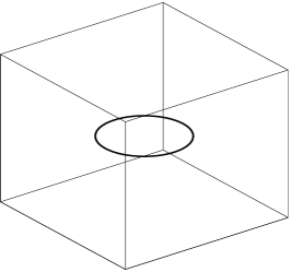
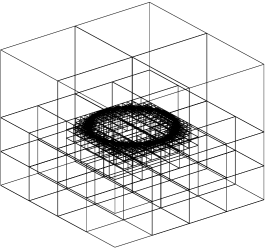
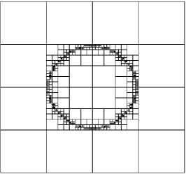
Figure 2: The complex octree structure required to map the vortex points for a single vortex loop (left panel) is plotted in the middle panel. The right panel shows the same structure in the $xy$-plane,at $z=0$.

At each time-step we have a set of orientated vortex points which represent the current position and direction of the vortex filaments. We first group the vortex points into a hierarchy of cubes which is arranged in a three-dimensional octree structure. The octree can be either be constructed top down or bottom up. We think that it is conceptually easier to work from the top down, repeatedly dividing the domain. To achieve this aim, we first divide the full computational box, the root cell, into eight cubes, and then continue to divide each cube into eight smaller ‘children’ cubes, until either a cube is empty or contains only one vortex point.

The numerical code, Qvort we have developed is written in FORTRAN 2003 and employs linked lists Brainerd to efficiently create the tree structure. In the code each cell in the tree is a node which, using pointers, links to the 8 children within the domain of the parent node. The main node is set to the full computational box, we then repeatedly call a recursive subroutine to allocate the points in this box to the main nodes child cells. This process is then repeated dividing the main nodes child cells until the hierarchical tree structure is created.

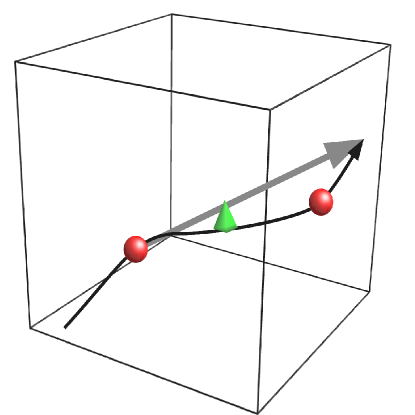
Figure 3: A cartoon of the calculation of the centre of circulation (green) triangle and the total circulation bold gray arrow. The (red) circles mark the position of the vortex points within a tree cell and the black line gives a representation of the vortex filament.

As we create the tree, we calculate the total circulation contained within each cube and the ‘center of circulation’ using the points that the cube contains. We denote the number of points the cube contains as $N_{\rm c}$, then the total circulation is given by

$$\mathbf{s}_{\Sigma}=\sum_{j=1}^{N_{\rm c}}(\mathbf{s}_{j+1}-\mathbf{s}_{j}).$$ (5)

Likewise the center of circulation is calculated as,

$$\bar{\mathbf{s}}=\frac{1}{N_{\rm c}}\sum_{j=1}^{N_{\rm c}}\mathbf{s}_{j}.$$ (6)

A schematic diagram for these quantities is displayed in Fig 3.

The time required for constructing the tree scales as $N\log(N)$, so it feasible (and essential) to ‘redraw’ the tree at each time-step. Fig. 1 illustrates this procedure in two dimensions for clarity. Fig. 2 shows the complex nature of the octree required for a single vortex ring in a three-dimensional calculation.

The enhanced speed of the tree method appears when we calculate the induced velocity at each vortex point $\mathbf{s}_{i}$. As opposed to the BS method, we only take the full contribution of points near to the vortex point in question. The induced velocity from far vortex points is an average contribution, hence the number of evaluations required per point is significantly smaller than $N-1$. Therefore for each point we must ‘walk’ the tree, and decide if a cell in the octree is sufficiently far.

This is done using the concept of the opening angle $\theta$. In their original work Barnes1986 , Barnes & Hut calculated $\theta$ by evaluating the distance of the center of vorticity from $\mathbf{s}_{i}$, which we denote as $d$. Since each cube in the octree has a known width $w$, then the opening angle is $\theta=w/d$. We then must define a critical (or maximum) opening angle $\theta_{\textrm{max}}$. If $\theta<\theta_{\textrm{max}}$ we accept the cube, and its contribution is used in computing the nonlocal contribution to the velocity via Eq. (3). The crucial difference between the full BS law and the tree approximation is that the vectors $\mathbf{p}$ and $\mathbf{q}$ must be redefined as $\mathbf{p}=\bar{\mathbf{s}}-\mathbf{s}_{i}$ and $\mathbf{q}=\mathbf{s}_{\Sigma}$. If $\theta_{max}=0$ then each cell contains one point at the most, and it is clear that $\mathbf{s}_{\Sigma}=\mathbf{s}_{j+1}-\mathbf{s}_{j}$, $\bar{\mathbf{s}}=\mathbf{s}_{j}$ and we recover $\mathbf{p}$ and $\mathbf{q}$ used in the full BS integral as one would expect.

If $\theta>\theta_{max}$, then we open the cube (assuming it contains more that one vortex point) and repeat the test on each of the child cubes that it contains. As a link list is used, from a programming point of view, it is relatively easy to start at the main node and follow the separate branches of the tree, at each stage evaluating whether the cells contribution can be used. The tree-walk ends when the contributions of all cubes have been evaluated. We note that the adjacent points are exempt from this walk, and their contribution is taken as in Eq. (2) so as to avoid the singularity.

A correction to this method was proposed by BarnesBarnes1994 ; Dubinski1996 to avoid errors which would arise if the center of vorticity is near the edge of the cube. This requires the calculation of the distance from the center of vorticity and the geometrical center of the cube, which we denote as $\zeta$. The test criteria then becomes $\theta=w/(d-\zeta)$. In Section IV we evaluate the improvement caused by this new criterion.

Whatever opening criterion is used, it is crucial to have a reasonable choice for $\theta_{\textrm{max}}$. If $\theta_{\textrm{max}}$ is too large, the discrepancy between the full BS integral and the tree approximation will damage to the accuracy of the simulation. In Section IV we shall also show how the errors in the calculation of the velocity at the vortex points depends on $\theta_{\textrm{max}}$.

In the next section we describe other necessary details of the vortex filament method which we used.

III Numerical methods

The numerical simulations presented here use a $3^{\rm rd}$ order Adams–Bashforth scheme. Given an evolution equation of the form $d\mathbf{s}/dt=\mathbf{v}$, the recursion formula is

$$\mathbf{s}_{i}^{n+1}=\mathbf{s}_{i}^{n}+\frac{\Delta t}{12}(23\mathbf{v}_{i}^{n}-16\mathbf{v}_{i}^{n-1}+5\mathbf{v}_{i}^{n-2})+\mathcal{O}(\Delta t^{4}).$$ (7)

where $\Delta t$ is the time-step and the superscript $n$ refers to the time $t_{n}=n\Delta t$ $(n=0,1,2,\cdots)$. Lower order schemes are used for the initial steps of the calculations, when older velocity values are not available.

As the vortex points move, the separation between neighbours along the same filament is not constant. In general this is not a problem, as we can use finite-difference schemes which work with an adaptive mesh size. However the distance between points sets the resolution of the calculation, therefore we must set some upper-bound on the distance between vortex points before we re-mesh the filaments by introducing new vortex points. Our criterion is the following: if the separation between two vortex points, $\mathbf{s}_{i}$ and $\mathbf{s}_{i+1}$, becomes greater than some threshold quantity $\delta$ (which we call the minimum resolution), we introduce a new vortex point at position $\mathbf{s}_{i^{\prime}}$ given by

$$\mathbf{s}_{i^{\prime}}=\frac{1}{2}(\mathbf{s}_{i}+\mathbf{s}_{i+1})+\left(\sqrt{R^{2}_{i^{\prime}}-\frac{1}{4}\ell_{i+1}^{2}}-R_{i^{\prime}}\right)\frac{\mathbf{s}_{i^{\prime}}^{{}^{\prime\prime}}}{|\mathbf{s}_{i^{\prime}}^{{}^{\prime\prime}}|},$$ (8)

where $R_{i^{\prime}}=|\mathbf{s}_{i^{\prime}}^{{}^{\prime\prime}}|^{-1}$. In this way $\mathbf{s}^{{}^{\prime\prime}}_{i^{\prime}}=(\mathbf{s}^{{}^{\prime\prime}}_{i}+\mathbf{s}^{{}^{\prime\prime}}_{i+1})/2$, that is to say the insertion of new vortex points preserves the curvature. This property is desirable, as the curvature of the filament directly affects the velocity field via Eq. (2). Our procedure is thus superior to simpler linear interpolation.

Conversely, vortex points are removed if their separation becomes less than $\delta/2$, ensuring that the shortest length-scale of the calculation remains fixed. This property is important, as the maximum time-step which can be used is related to this length-scale. In the long-wavelength approximation ($ka_{0}\ll 1$), the angular frequency of a Kelvin wave, along a straight vortex is

$$\omega\approx-\frac{\kappa k^{2}}{4\pi}\left[\ln 2/(ka_{0})-\gamma\right],$$ (9)

where $\gamma=0.5772$ is Euler’s constant. Hence the timescale for the fastest motions, with a maximum wavenumber $k_{\mathrm{max}}=4\pi/\delta$, is

$$(\omega_{\mathrm{max}})^{-1}\approx\frac{\pi(\delta/2)^{2}}{4\kappa\ln(\delta/2\pi a_{0}-\gamma)},$$ (10)

thus a reasonable maximum time-step that can be used is given by

$$\Delta t<\frac{(\delta/2)^{2}}{\kappa\log(\delta/2\pi a_{0})}.$$ (11)

We note that at finite temperatures this condition may be relaxed as mutual friction will tend to dampen Kelvin waves. Setting a consistent minimum separation between vortex points makes the numerical resolution of the calculation transparent, and prevents the creation of too short length-scales which would considerably slow down the calculation.

In order to model any turbulent system we must pay particular attention to the dissipation of kinetic energy. Even at very low temperatures, in the absence of mutual friction with the normal fluid, there are still mechanisms which dissipate the kinetic energy of quantised vortices: reconnections, decay of very small vortex loops and direct phonon emission.

Using the GPE condensate model, Leadbeater & al Leadbeater2001 showed that, at vortex reconnection events, a small amount of kinetic energy is transformed into acoustic energy of a rarefaction pulse which moves away. Since our model neglects sound waves and it would be impractical to determine with accuracy very small changes of kinetic energy, we interpret this dissipation of kinetic energy as a reduction of vortex length, essentially using length as a proxy for energy.

We model reconnection events algorithmically in the following way. If two discretization points, which are not neighbours, become closer to each other than the local discretization distance, a numerical algorithm reconnects the two filaments by simply switching flags for the vortex points in front and behind the filament, subject to the criterion that the total length decreases. Self-reconnections (which can arise if a vortex filament has twisted and coiled by a large amount) are treated in the same way. Since reconnections involve only anti-parallel filaments, prior to reconnection we form local (unit) tangent vectors $\mathbf{s}^{\prime}$, and, using the inner product, we check that the two filaments are not parallel.

Clearly, testing for possible reconnections requires a distance evaluation between a vortex point and the vortex points in the vicinity. The most efficient way to do this is within the tree-walk itself, creating a linked list of all vortex points within a radius of $\delta/2$ from a vortex point in question. This avoids the need to re-loop over all discretization points, which would involve approximately $N^{2}$ operations.

We distinguish two kinds of phonon emissions. The condensate model shows that very small vortex loops, of radius of the order of $a_{0}$, which move at speed close to the speed of sound, are unstable and decay into soundJones-Roberts . It would not be practical to mesh vortex filaments down to this atomic scale, so we remove any small vortex loop with less than five discretization points.

Phonon emission can also be induced by very short Kelvin waves which rotate rapidly Vinen2001 ; Leadbeater2002 . Again, since we do not mesh filaments down to this scale, we remove vortex points if the local wavelength is smaller than a specified value tree . Since our smallest length-scale is maintained at $\delta/2$, the maximum curvature is of the order of $2/\delta$. We proceed in this way: at each time-step we compute the local curvature $C(\xi)=|\mathbf{s}^{\prime\prime}|$ at each vortex point. If, at some location along a vortex filament, the local curvature exceeds the critical value $1.9/\delta~{}\mathrm{cm}^{-1}$ ($95\%$ of the maximum value $2/\delta$), this vortex point is removed, smoothing the vortex filament locally. This loss of length as a proxy of energy is our model of phonon emission in the low temperature limit.

We approximate all spatial derivatives using $4^{\rm th}$ order finite difference schemes which account for varying mesh sizes along the vortex filaments Gamet1999 . A high-order scheme is desirable as the spatial derivatives enter into the equation of motion via, Eq. (2). Let $\mathbf{s}_{i}$ be the $i^{\rm th}$ point on the vortex filament; the two points behind have positions $\mathbf{s}_{i-2}$ and $\mathbf{s}_{i-1}$, and the two points in front have positions $\mathbf{s}_{i+1}$ and $\mathbf{s}_{i+2}$. We denote $\ell_{i-1}=|\mathbf{s}_{i-1}-\mathbf{s}_{i-2}|$, $\ell_{i}=|\mathbf{s}_{i}-\mathbf{s}_{i-1}|$, $\ell_{i+1}=|\mathbf{s}_{i+1}-\mathbf{s}_{i}|$, and $\ell_{i+2}=|\mathbf{s}_{i+2}-\mathbf{s}_{i+1}|$. We have:

$$\mathbf{s}_{i}^{\prime}=A_{1i}\mathbf{s}_{i-2}+B_{1i}\mathbf{s}_{i-1}+C_{1i}\mathbf{s}_{i}+D_{1i}\mathbf{s}_{i+1}+E_{1i}\mathbf{s}_{i+2},$$ (12)

where the coefficients $A_{1i}$, $B_{1i}$, $C_{1i}$, $D_{1i}$ and $E_{1i}$ are given by,

$$A_{1i}=\frac{\ell_{i}\ell_{i+1}^{2}+\ell_{i}\ell_{i+1}\ell_{i+2}}{\ell_{i-1}(\ell_{i-1}+\ell_{i})(\ell_{i-1}+\ell_{i}+\ell_{i+1})(\ell_{i-1}+\ell_{i}+\ell_{i+1}+\ell_{i+2})}$$ (13)

$$B_{1i}=\frac{-\ell_{i-1}\ell_{i+1}^{2}-\ell_{i}\ell_{i+1}^{2}-\ell_{i-1}\ell_{i+1}\ell_{i+2}-\ell_{i}\ell_{i+1}\ell_{i+2}}{\ell_{i-1}\ell_{i}(\ell_{i}+\ell_{i+1})(\ell_{i}+\ell_{i+1}+\ell_{i+2})}$$ (14)

$$C_{1i}=-(A_{1i}+B_{1i}+D_{1i}+E_{1i})$$ (15)

$$D_{1i}=\frac{\ell_{i-1}\ell_{i}\ell_{i+1}+\ell_{i}^{2}\ell_{i+1}+\ell_{i-1}\ell_{i}\ell_{i+2}+\ell_{i}^{2}\ell_{i+2}}{\ell_{i+1}\ell_{i+2}(\ell_{i}+\ell_{i+1})(\ell_{i-1}+\ell_{i}+\ell_{i+1})}$$ (16)

$$E_{1i}=\frac{-\ell_{i+1}\ell_{i}^{2}-\ell_{i-1}\ell_{i}\ell_{i+1}}{\ell_{i+2}(\ell_{i+1}+\ell_{i+2})(\ell_{i}+\ell_{i+1}+\ell_{i+2})(\ell_{i-1}+\ell_{i}+\ell_{i+1}+\ell_{i+2})}$$ (17)

Similarly we have:

$$\mathbf{s}_{i}^{\prime\prime}=A_{2i}\mathbf{s}_{i-2}+B_{2i}\mathbf{s}_{i-1}+C_{2i}\mathbf{s}_{i}+D_{2i}\mathbf{s}_{i+1}+E_{2i}\mathbf{s}_{i+2},$$ (18)

where the coefficients $A_{2i}$, $B_{2i}$, $C_{2i}$, $D_{2i}$ and $E_{2i}$ are given by

$$A_{2i}=\frac{2[-2\ell_{i}\ell_{i+1}+\ell_{i+1}^{2}-\ell_{i}\ell_{i+2}+\ell_{i+1}\ell_{i+2}]}{\ell_{i-1}(\ell_{i-1}+\ell_{i})(\ell_{i-1}+\ell_{i}+\ell_{i+1})(\ell_{i-1}+\ell_{i}+\ell_{i+1}+\ell_{i+2})}$$ (19)

$$B_{2i}=\frac{2[2\ell_{i-1}\ell_{i+1}+2\ell_{i}\ell_{i+1}-\ell_{i+1}^{2}+\ell_{i-1}\ell_{i+2}+\ell_{i}\ell_{i+2}-\ell_{i+1}\ell_{i+2}]}{\ell_{i-1}\ell_{i}(\ell_{i}+\ell_{i+1})(\ell_{i}+\ell_{i+1}+\ell_{i+2})}$$ (20)

$$C_{2i}=-(A_{2i}+B_{2i}+D_{2i}+E_{2i})$$ (21)

$$D_{2i}=\frac{2[-\ell_{i-1}\ell_{i}-\ell_{i}^{2}+\ell_{i-1}\ell_{i+1}+2\ell_{i}\ell_{i+1}+\ell_{i-1}\ell_{i+2}+2\ell_{i}\ell_{i+2}]}{\ell_{i+1}\ell_{i+2}(\ell_{i}+\ell_{i+1})(\ell_{i-1}+\ell_{i}+\ell_{i+1})}$$ (22)

$$E_{1i}=\frac{2[\ell_{i-1}\ell_{i}+\ell_{i}^{2}-\ell_{i-1}\ell_{i+1}-2\ell_{i}\ell_{i+1}]}{\ell_{i+2}(\ell_{i+1}+\ell_{i+2})(\ell_{i}+\ell_{i+1}+\ell_{i+2})(\ell_{i-1}+\ell_{i}+\ell_{i+1}+\ell_{i+2})}$$ (23)

Note that if we set $\ell_{i-1}=\ell_{i}=\ell_{i+1}=\ell_{i+2}=h$, then the above expressions reduce to familiar finite-difference schemes for a uniform mesh:

$$\mathbf{s}_{i}^{\prime}=\frac{1}{12h}(\mathbf{s}_{i-2}-8\mathbf{s}_{i-1}+8\mathbf{s}_{i+1}-\mathbf{s}_{i+2})+\mathcal{O}(h^{4}),$$ (24)

$$\mathbf{s}_{i}^{\prime\prime}=\frac{1}{12h^{2}}(-\mathbf{s}_{i-2}+16\mathbf{s}_{i-1}-30\mathbf{s}_{i}+16\mathbf{s}_{i+1}-\mathbf{s}_{i+2})+\mathcal{O}(h^{4}).$$ (25)

The final issues to address in this section is the boundary conditions used in the simulations and how they are implemented. All numerical simulations presented here were performed with periodic boundary conditions. The computational domain was a cube. If a vortex point leaves the domain, then it is simply re-inserted at the opposite side of the cube. The presence of periodic boundary conditions affects the calculation of the distance between two vortex points (two vortex points point at the opposite end of the domain may be actually close to each other). We must also use periodic ‘wrapping’ to ensure that the velocity field is periodic; in theory we should wrap the cube with an infinite number of copies in all directions. In practice, we only apply a single layer of wrapping, which still requires a very large amount of numerical evaluations. If we used the BS law, a single layer of wrapping would require $27N^{2}$ evaluations per time-step. Fortunately again the tree method eases the amount of numerical work, as the computational domain is wrapped with copies of the octree we have already computed. Walking each of these trees, as well as the tree for the main domain, does not require a significant increase of CPU time.

IV Tests of the tree algorithm

We now test the error associated with the use of the tree approximation, and show that, with an appropriate choice of $\theta_{\textrm{max}}$, the discrepancy between using the tree algorithm and the full BS law is very small. All tests are carried out in a periodic cube of side $0.1~{}\rm cm$. The minimum resolution is set at $\delta=0.001$cm, and the time-step is $\Delta t=10^{-5}$s. For our first test we consider a system of ten random vortex loops with an increasing number of vortex points (hence increasing radius). We determine the CPU time required for evolving the system for one hundred time-steps as a function of $\theta$; the results are presented in Fig. 4. It is apparent that even for very small maximum opening angles, $\theta_{\textrm{max}}$, there is a huge increase in CPU speed, and for larger values of $\theta_{\textrm{max}}$ the $N\log N$ scaling is apparent.

\psfrag{N}{$N$}\psfrag{t}{time(s)}\psfrag{s1}{$\mathcal{O}(N^{2})$}\psfrag{s2}{$\mathcal{O}(N\log N)$}\includegraphics[width=260.17464pt]{timing.eps}

Figure 4: The CPU time required for one hundred time-steps, plotted as a function of the number of vortex points $N$. The calculations were performed on an single processor with a clock speed of $2.53~{}\rm GHz$. The symbols represent different values of $\theta_{\textrm{max}}$ as follows: triangles, $\theta_{\textrm{max}}=0.6$, asterisks, $\theta_{\textrm{max}}=0.4$, squares, $\theta_{\textrm{max}}=0.2$, and circles, $\theta_{\textrm{max}}=0.$ (that is, the full BS calculation).

\psfrag{theta}{$\theta_{\textrm{max}}$}\psfrag{ebar}{$\bar{\epsilon}$}\includegraphics[width=260.17464pt]{theta_error.eps}

Figure 5: The scaling of the mean relative percentage error in the velocity field, $\bar{\epsilon}$, evaluated at discretization points plotted as a function of $\theta_{\textrm{max}}$. The dashed line corresponds to the original opening angle criterion Barnes1986 and the solid line shows the performance of the correction of Barnes Barnes1994 .

The second test consists in determining the discrepancies between the ‘true’ velocity field (obtained using the BS law) and the velocity filed obtained with the tree method, as a function of $\theta_{\textrm{max}}$. Let $\mathbf{v}_{i,BS}$ be the the velocity at the discretization point $\mathbf{s}_{i}$ obtained using the BS integral, and $\mathbf{v}_{i,T}$ the corresponding velocity obtained using the tree method. We define the mean relative percentage error of the tree method as

$$\bar{\epsilon}=100\times\frac{1}{N}\sum_{i=1}^{N}\frac{|\mathbf{v}_{i,BS}-\mathbf{v}_{i,T}|}{|\mathbf{v}_{i,BS}|}.$$ (26)

Again, we use a system of 10 randomly oriented and positioned vortex loops in the same periodic box, each vortex loop discretized into 200 vortex points. Figure 5 shows how $\bar{\epsilon}$ varies as a function of $\theta_{\textrm{max}}$, for both the original tree opening criterion and the correction of Barnes. Whilst the improvement is modest, since the extra computational cost is negligible, hereafter we include Barnes’s modification.

The next test investigates how this error varies as a function of $N$ for a fixed value of $\theta_{\textrm{max}}$. This test is particularly important in view of computing very dense vortex tangles, which are not accessible using the exact BS law. As before, we consider a system of 10 random vortex loops with an increasing number of vortex points in the same periodic box, and compute $\bar{\epsilon}$. Figure 6 shows the results for fixed $\theta_{\textrm{max}}=0.4$. It is apparent that the error grows with the number of vortex points, but its magnitude is still small considering the advantages of the tree method. We obtain the same result with a different set up to increase $N$: we fix the vortex loop size but increase the number of vortex loops.

\psfrag{N}{$N$}\psfrag{ebar}{$\bar{\epsilon}$}\includegraphics[width=260.17464pt]{error_vs_N.eps}

Figure 6: The mean relative percentage error of the tree approximation for a fixed maximum opening angle, $\theta_{\textrm{max}}=0.4$, with an increasing number of discretization points and therefore vortex length in the system.

In the previous tests we have only considered the errors at a single time-step of a simulation. It is important to quantify how the difference between the exact BS law and the tree method varies in time. For this test we deliberately choose a vortex configuration which the LIA fails to accurately model, namely two ‘leap-frogging’ vortices.

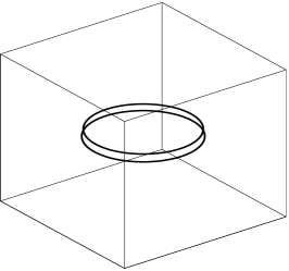
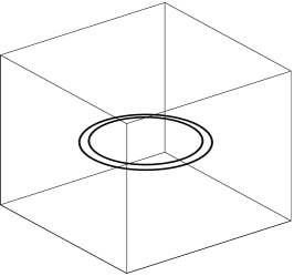
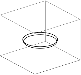
Figure 7: A system of leap-frogging vortices, each loop contains 200 vortex points with $\delta=0.001$cm, the mean separation is $0.00075$cm giving each loop a radius of $0.024~{}\rm cm$. These snapshots are taken from a tree code simulation with $\theta_{\textrm{max}}=0.4$.

The initial condition consists of two co-axial vortex rings set in the $xy$-plane, separated by a small distance in the $z$ direction. Given the orientation of the vortex lines, the local velocity component - see Eq. (2) - drives the vortices in the negative $z$ direction. The non-local velocity component makes the vortex ring which is initially behind to squeeze through the vortex ring which is in front, overtaking it; the process repeats over and over again, in a leap-frogging fashion (note that the vortices maintain the circular shape). This remarkable behaviour is visible in Fig. 7. We stress that this behaviour is not captured by the LIA. We repeat the calculation using the exact BS law, keeping the same number $N$ of vortex points and the same minimum resolution $\delta$. We then quantity the difference between the tree method and the BS law by computing

$$\bar{D_{s}}(t)=\frac{1}{N}\sum_{i=1}^{N}\frac{|\mathbf{s}_{i,BS}(t)-\mathbf{s}_{i,T}(t)|}{\delta},$$ (27)

where $\mathbf{s}_{i,BS}$ is the position of the $i^{\textrm{th}}$ vortex point in the BS calculation, and $\mathbf{s}_{i,T}$ is the corresponding position in the tree method calculation. The temporal duration of these calculations captures four separate leap-frogging events. Figure 8 shows the evolution of $\bar{D_{s}}$ for two different values of $\theta_{\textrm{max}}$: $0.4$ and $0.8$. It is apparent that in both cases the difference between the tree method and the exact BS evolution is small (smaller than the minimum discretization level $\delta$), particularly for $\theta_{\textrm{max}}=0.4$.

\psfrag{t}{$t$}\psfrag{diste}{$\bar{D_{s}}$}\includegraphics[width=260.17464pt]{dist_error.eps}

Figure 8: The evolution of the normalised distance error statistic $\bar{D_{s}}$ (see Eq. (27)), for a system of leap-frogging vortex rings, plotted as a function of $t$ (seconds). The solid line corresponds to a simulation with $\theta_{\textrm{max}}=0.4$, and the dashed line to $\theta_{\textrm{max}}=0.8$.

V Counterflow simulations

Having benchmarked the tree method for simple vortex configurations, we change our focus to numerical simulations of quantum turbulence. We concentrate our attention to turbulence sustained by the relative motion (counterflow) of normal fluid and superfluid components, driven by a heat flow at non nonzero temperature. This form of turbulence which has no analogy in ordinary fluids was originally studied experimentally by Vinen Vinen1957 , and, numerically, by Schwarz Schwarz . Counterflow turbulence has been recently re-examined by Adachi & al. Adachi2010 , who compared results obtained using the LIA (as in the pioneering work of SchwarzSchwarz ) and the full BS law. Counterflow turbulence is particularly suitable for testing the tree method, as Adachi & al. used it to discuss the shortcoming of LIA. We want to make sure that the tree method does not suffer from the same problems of the LIA.

At finite temperatures we must account for the mutual friction between the superfluid and the normal fluid. The equation of motion at position $\mathbf{s}$ is given by

$$\frac{d\mathbf{s}}{dt}=\mathbf{v}_{s}+\alpha\mathbf{s}^{\prime}\times(\mathbf{v}_{n}-\mathbf{v}_{s})-\alpha^{\prime}\mathbf{s}^{\prime}\times\left[\mathbf{s}^{\prime}\times(\mathbf{v}_{n}-\mathbf{v}_{s})\right],$$ (28)

where $\alpha$, $\alpha^{\prime}$ are temperature dependent friction coefficients Barenghi1983 ; Barenghi1998 , $\mathbf{v}_{n}$ is the normal fluid’s velocity, and the velocity $\mathbf{v}_{s}$ is calculated using the tree approximation to the de-singularised BS integral. As usual, the evolution includes the algorithmical vortex reconnection procedure.

The calculation is performed in a periodic cube with sides of length $0.1~{}\rm cm$ as done by Adachi et al. Adachi2010 . Superfluid and normal fluid velocities $\mathbf{v}_{n}$ and $\mathbf{v}_{s}$ are imposed in the positive and negative $x$ directions respectively, where $v_{ns}=|\mathbf{v}_{n}-\mathbf{v}_{s}|$ is proportional to the applied heat flux. Simulations are performed with the same numerical resolution $\delta=8\times 10^{-4}~{}\rm cm$ and time-step $\Delta t=10^{-4}~{}\rm s$ as used by Adachi et al. at various value of $v_{n}$ and $T$. Whereas Adachi et al. used the BS law, we use our tree method with $\theta_{\textrm{max}}=0.4$. The number of vortex points used in these calculations is not large, in order to overlap with calculations which used the BS law:) for example a typical value is $N\approx 6000$ at $v_{ns}=0.572~{}\rm cm/s$ and $T=1.9~{}\rm K$. It must be stressed that, as in the works of Schwarz and Adachi et al. , the back-reaction of the superfluid vortex lines onto the normal fluid velocity is neglected (an effect which may be significant at low temperatures). The initial condition consists of six vortex loops set at random locations, as for Adachi et al. . We find that the results do not depend on the initial condition.

During the evolution we monitor the vortex line density

$$L=\frac{1}{V}\int_{\mathcal{L}}d\xi,$$ (29)

where $V$ is the volume of the computational domain and $\mathcal{L}$ is the entire vortex configuration.

\psfrag{t}{$t$}\psfrag{L}{$L$}\includegraphics[width=173.44534pt]{CFLD2.eps}

\psfrag{t}{$t$}\psfrag{L}{$L$}\psfrag{L}{$\sqrt{L}$}\psfrag{v}{$v_{ns}$}\includegraphics[width=173.44534pt]{CFLvV2.eps}

Figure 9: Left: The evolution of the vortex line density $L$ ($\rm cm^{-2}$) vs time $t$ ($\rm s$) for counterflow simulations at $1.9~{}\rm K$ for four counterflow velocities: dashed-dotted, $v_{ns}=0.2~{}\rm cm/s$, dashed, $v_{ns}=0.4~{}\rm cm/s$, solid (black), $v_{ns}=0.6~{}\rm cm/s$, and solid (grey), $v_{ns}=0.8~{}\rm cm/s$. Right: The plot of the vortex line density $L$ ($\rm cm^{-2}$) vs $v_{ns}$ ($\rm cm/s$) confirms that the saturated line density scales according to $L\sim v_{ns}^{2}$.

We find that, after an initial transient, the vortex line density saturates to a statistical steady state value, see Figure 9 (left), which agrees well with the value reported by Adachi et al. in their Figure 2 at the same temperature and counterflow velocity. Figure 9 (right) shows the expected relation $\sqrt{L}\sim v_{ns}$ between the steady state value of $L$ and the driving counterflow. More precisely, we obtain $\gamma=140.8$, which compares well with $\gamma=140.1$ obtained by Adachi et al. , where $L=\gamma^{2}v_{ns}^{2}$.

Another important quantity considered by Schwarz and Adachi et al. is the anisotropy parameter

$$l_{||}=\frac{1}{VL}\int_{\mathcal{L}}\left[1-(\mathbf{s}^{\prime}\cdot\hat{\mathbf{r}}_{||})^{2}\right]d\xi,$$ (30)

where $\hat{\mathbf{r}}_{||}$ is the unit vector parallel in the direction of the normal fluid. Figure 10 (right) shows that $l_{||}$ is almost independent of $v_{ns}$, in agreement with experiments and with the numerical calculations of Adachi et al. performed using the full BS law (shown in their Fig. 7). For example at $v_{ns}=0.55~{}\rm cm/s$ we have $I_{||}\approx 0.83$, compared to $0.80$ - $0.85$ of Adachi et al. . Figure 10 also shows that this anisotropy is not captured by the LIA.

A final qualitative test is shown in Fig. 11: the left panel shows the bundling of vortex lines wrongly predicted by the LIA, and the right panel shows the vortex tangle computed using the tree method, in agreement with Adachi et al. .

\psfrag{lpara}{$l_{||}$}\psfrag{t}{$t$}\includegraphics[width=173.44534pt]{LIA_lpara_vs_t.eps}

\psfrag{lpara}{$l_{||}$}\psfrag{t}{$t$}\psfrag{lpara}{$l_{||}$}\psfrag{v}{$v_{ns}$}\includegraphics[width=173.44534pt]{lpara_vs_v2.eps}

Figure 10: Left: The anisotropy parameter $l_{||}$ plotted as a function of time $t$ ($s$) for the LIA simulation (grey) and for the tree method (black) with $\theta_{\textrm{max}}=0.4$. Right: The steady-state $l_{||}$ parameter plotted for four different normal fluid velocities $v_{ns}$ ($\rm cm/s$) plotted with error bars (calculated from temporal fluctuations) for the tree method only. These results are in excellent agreement with those of Adachi et al. Adachi2010

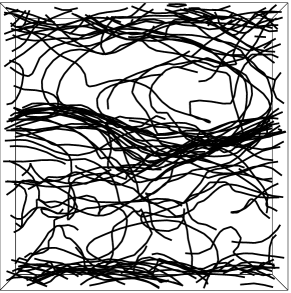
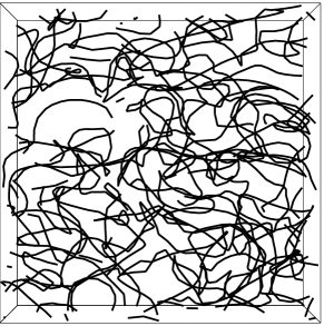
Figure 11: Views of the tangles from the top of the computational domain in the $xy$-plane for the LIA simulation (left) and the tree method (right). The domain is a cube with sides of length $0.2~{}\rm cm$; the imposed normal velocity is $v_{ns}=0.5~{}\rm cm/s$ and $T=1.6~{}\rm K$. Note the stratified nature of the tangle wrongly predicted by the LIA.

VI Conclusions

We conclude that the tree method is an ideal tool to perform numerical simulations of quantum turbulence. It does not suffer from the known shortcoming of the LIA, retaining to a good approximation the nonlocal interaction which is typical of the exact BS law. Unlike the BS law, whose computational cost scales as $N^{2}$ where $N$ is the number of discretization points, the cost of tree method scales as $N\log{(N)}$, thus making possible numerical calculations of intense vortex tangles for a sufficiently long time. Finally, the tree method can be further speeded up by parallelization.

References

- (1) R.J. Donnelly, Quantized Vortices In Helium II, Cambridge University Press, Cambridge (1991)
- (2) C.F. Barenghi & Y.A. Sergeev (eds.), Vortices and Turbulence at Very Low Temperatures, CISM Courses and Lecture Notes, Springer (2008)
- (3) W. P. Halperin & M. Tsubota (eds.), Progress in Low Temperature Physics: Quantum Turbulence, vol. XVI, Elsevier (2008)
- (4) J. Maurer & P. Tabeling, Europhys. Lett. 43, 29 (1998)
- (5) P.-E. Roche, P. Diribarne, T. Didelot, O. Français, L. Rousseau, & H. Willaime, Europhys. Lett. 77, 66002 (2007)
- (6) M. Blaz̆ková, D. Schmoranzer, L. Skrbek, & W. F. Vinen Phys. Rev. B 79, 054522 (2009)
- (7) M.R. Smith, R.J. Donnelly, N. Goldenfeld, & W.F. Vinen, Phys. Rev. Lett. 71, 2583 (1993)
- (8) W.F. Vinen, Proc. Roy. Soc. A240, 114 (1957); W.F. Vinen, Proc. Roy. Soc. A240, 128 (1957); W.F. Vinen, Proc. Roy. Soc. A242, 494 (1957); W.F. Vinen, Proc. Roy. Soc. A243, 400 (1957)
- (9) M.S. Paoletti, M.E. Fisher, K.R. Sreenivasan, and D.P. Lathrop, Phys. Rev. Lett. 101 154501 (2008)
- (10) P M. Walmsley & A.I. Golov, Phys. Rev. Lett. 100, 245301 (2008)
- (11) V.B. Eltsov, R. de Graaf, P.J. Heikkinen, J.J. Hosio, R. Hänninen, M. Krusius, & V. S. L’vov, Phys. Rev. Lett. 105, 125301 (2010)
- (12) D.I. Bradley, S.N. Fisher, A.M. Guénault, R.P. Haley, G.R. Pickett, D. Potts & V. Tsepelin, Nature Physics 7, 473 (2011)
- (13) E.A.L. Henn, J.A. Seman, G. Roati, K.M.F. Magalhães, and V.S. Bagnato, Phys. Rev. Lett. 103, 045301 (2009)
- (14) W.F. Vinen & J.J. Niemela, J. Low Temp. Phys. 128, 167 (2002) and Erratum, 129, 213 (2002)
- (15) V. S. L’vov, S. V. Nazarenko & L. Skrbek, J. Low Temp. Phys. 145 125 (2006)
- (16) G.P. Bewley, D.P. Lathrop, & K.R. Sreenivasan, Nature 441, 588 (2006)
- (17) T. Zhang & S.W. Van Sciver, Nature Physics 1, 36 (2005)
- (18) D.I. Bradley, S.N. Fisher, A.M. Guénault, M.R. Lowe, G.R. Pickett, A. Rahm, & R.C.V. Whitehead, Phys. Rev. Lett. 93, 235302 (2004)
- (19) W. Guo, S.B. Cahn, J.A. Nikkel, W.F. Vinen, & D.N. McKinsey Phys. Rev. Lett. 105, 045301 (2010)
- (20) K.W. Schwarz, Phys. Rev. B 38, 2398 (1988)
- (21) D.C. Samuels, Phys. Rev. B 46, 11714 (1992)
- (22) A.T.A.M. de Waele and R.G.K.M. Aarts, Phys. Rev. Lett. 72, 482 (1994)
- (23) C.F. Barenghi, D.C. Samuels, G.H. Bauer, & R.J. Donnelly, Phys. Fluids 9, 2631 (1997)
- (24) M. Tsubota, T. Araki, & C.F. Barenghi, Phys. Rev. Lett. 90, 205301 (2003)
- (25) V.B. Eltsov, A.I. Golov, R. de Graaf, R. Hänninen, M. Krusius, V.S. L’vov, & R. E. Solntsev, Phys. Rev. Lett. 99, 265301 (2007)
- (26) L. Kondaurova & S.K. Nemirovskii, J. Low Temp. Phys. 138, 555 (2005)
- (27) D. Kivotides, J.C. Vassilicos, D.C. Samuels, & C.F. Barenghi, Phys. Rev. Lett. 86, 3080 (2001).
- (28) K. Morris, J. Koplik, & D.W.I. Rouson, Phys. Rev. Lett. 101, 015301 (2008)
- (29) D. Kivotides, Phys. Rev. Lett. 96, 175301 (2006)
- (30) A.W. Baggaley & C.F. Barenghi, Phys. Rev. B 83, 134509 (2011)
- (31) A.W. Baggaley & C.F. Barenghi, Phys. Rev. B 84, 020504 (2011)
- (32) D. Kivotides, C.F. Barenghi, & Y.A. Sergeev, Phys. Rev. B 77 014527 (2008)
- (33) A.P. Finne, T. Araki, R. Blaauwgeers, V.B. Eltsov, N.B. Kopnin, M. Krusius, L. Skrbek, M. Tsubota, G.E. Volovik, Nature 424, 1022 (2003)
- (34) P.G. Saffman, Vortex Dynamics, Cambridge University Press (1992)
- (35) J. Koplik and H. Levine, Phys. Rev. Lett. 71 1375 (1993)
- (36) G.P. Bewley, M.S. Paoletti, K.R. Sreenivasan and D.P. Lathrop, P.N.A.S. 105, 13707 (2008)
- (37) R. Tebbs, A.J. Youd and C.F. Barenghi, J. Low Temp. Physics 162, 314 (2011)
- (38) R.M. Kerr Phys. Rev. Lett. 106, 224501 (2011)
- (39) M. Kursa, K. Bajer, & T. Lipniacki, Phys. Rev. B 83, 014515 (2011)
- (40) C.F. Barenghi, Physica D, 237 2195 (2008)
- (41) L.S. Da Rios, Rend. Circ. Mat. Palermo 22, 117 (1905)
- (42) R.J. Arms and F.R. Hama, Phys. Fluids 8, 553 (1965)
- (43) R.L. Ricca, D.C. Samuels, & C.F. Barenghi, J. Fluid Mech. 391, 29 (1999)
- (44) G. Boffetta, A. Celani, D. Dezzani, J. Laurie & S. Nazarenko, J. Low Temp. Phys 156, 193 (2009)
- (45) H. Adachi, S. Fujiyama, & M. Tsubota, Phys. Rev. B, 81, 104511 (2010)
- (46) V. Springel, Ann. Review Astronomy and Astrophysics, 48, 391 (2010)
- (47) D.Kivotides, Phys. Rev. Lett.,76, 054503 (2007)
- (48) E.Kozik & B. Svistunov, Phys. Rev. B,94, 025301 (2005)
- (49) J. Barnes & P. Hut, Nature 324, 446 (1986)
- (50) E. Bertschinger, Ann. Review Astronomy and Astrophysics 36, 599 (1998)
- (51) V.Springel, S.D.M. White, A. Jenkins, C.S. Frenk, N. Yoshida, L. Gao, J. Navarro, R. Thacker, D. Croton, J. Helly, J.A. Peacock, S. Cole, P. Thomas, H. Couchman, A. Evrard, J. Colberg, & F. Pearce, Nature 435, 629 (2005)
- (52) J.K. Salmon, California Inst. of Tech., Pasadena (1991)
- (53) W.S.Brainerd, Guide to Fortran 2003 Programming, Springer Verlag, Berlin (2009)
- (54) J. Dubinski, New Astronomy 1, 133 (1996)
- (55) J. Barnes, Computational Astrophysics, Springer Verlag, Berlin (1994)
- (56) C.F. Barenghi, R.J. Donnelly, & W.F. Vinen, J. Low Temp. Phys. 52, 189 (1983)
- (57) R.J. Donnelly & C.F. Barenghi, J. Phys. Chem. Reference Data 27, 1217 (1998)
- (58) M. Leadbeater, T. Winiecki, D.C. Samuels, C.F. Barenghi & C.S. Adams, Phys. Rev. Letters 86, 1410 (2001)
- (59) C.A. Jones & P.H. Roberts, J. Phys. A (Mathematical and General) 15, 2599 (1982)
- (60) W.F. Vinen, Phys. Rev. B 64, 134520 (2001)
- (61) M. Leadbeater, D.C. Samuels, C.F. Barenghi and C.S. Adams, Phys. Rev. A 67, 015601 (2002)
- (62) L. Gamet, F. Ducros, F. Nicoud and T. Poinsot, Int. J. Numerical Methods in Fluids, 29, 159 (1999)