Reply to Comment on “Critical analysis of a variational method used to describe molecular electron transport”

Abstract

We show that the failure of the Delaney-Greer (DG) variational ansatz for transport demonstrated by us in Phys. Rev. B 80, 165301 (2009) (I) is not related to an unsuitable constraint that prevents a broken time-reversal symmetry or to real orbitals, as DG incorrectly claim. The complex orbitals suggested by them as a way-out solution merely represent a particular case of the general case considered by us in I, which do not in the least affect our conclusion. In conjunction with the issues raised by the DG’s Comment, we show that the DG Wigner conditions can erroneously constrain outgoing and not incoming charge carriers and present an example revealing that the sign of the “momentum” $P$ of the Wigner function $f(q,P)$ is not necessarily associated with the direction of motion in the real world. We also discuss a general reason why transport approaches which, like the DG’s, are solely based on information on an isolated nanocluster are incorrect.

I Introduction

In their Comment, GreerComment:10 Delaney and Greer (DG) claim that the unphysical result (current $J=0$) presented by us in Ref. Baldea:2009c, (hereafter, I) as evidence against their variational approach DelaneyGreer:04a is due to the fact (i) that our constraints (electronic populations) prevent a broken time-reversal symmetry, and (ii) that we used real orbitals, which concomitantly constrain incoming and outgoing electrons. Further, DG accept that our idea to constrain populations “is an interesting alternative to the Wigner function” (WF), but (iii) argue that to get $J\neq 0$ it is essential to use complex orbitals, like those obtained by applying periodic boundary conditions (pBCs) for electrodes. By using the superscript $DG$ and by referring to their work,DelaneyGreer:04a which we amply criticized Baldea:2008b ; Baldea:2009c ; Baldea:2010g they aim to convey the false impression that they used such complex orbitals previously.

Responding briefly, claim (i) is incorrect, claim (ii) has absolutely no real basis, while claim (iii) does not mender their variational approach; the complex orbitals discussed by them solely represent a particular case of the general case of I and do not in the least change the unphysical linear response current $J=0$.

II Rebuttal of the criticism that population constraints prevent a broken time-reversal symmetry

DG argue that the unphysical result ($J=0$) deduced in I is the consequence of our unsuitable choice of constraints, namely the particle number operators. They (incorrectly) claim that constraining real particle number operators does not break time-reversal symmetry, and for this very reason the current vanishes even beyond the linear response limit examined in I.

We shall immediately show that this is not true: our constraints allow a broken time-reversal symmetry. The fact that this symmetry is not broken is the result of the defective DG variational ansatz (constrained energy minimization at zero temperature). Below, we shall only discuss the particular constraint $Q_{\kappa}=n_{\kappa}\equiv\alpha_{\kappa}^{\dagger}\alpha_{\kappa}$ mentioned in the Comment. Let us consider a general many-body state, $\left|\Psi\right\rangle=\sum_{n}A_{n}\left|\Psi_{n}\right\rangle$, expanded in terms of the complete set of the real eigenstates of the Hamiltonian $H$ of the finite transport cluster without external bias ($V=0$), $H|\Psi_{n}\rangle=E_{n}|\Psi_{n}\rangle$. Notice that this exact expansion is just in the spirit of the DG approach, which is based on a configuration interaction (CI), albeit approximate expansion [cf. Eq. (1) of Ref. DelaneyGreer:04a, ]. The expansion coefficients $A_{n}$ are allowed to be complex. Accepting the DG challenge, we consider now the general response instead of the linear limit of I. We do no more single out the ground state $|\Psi_{0}\rangle$, unlike e. g., Eq. (10) of I, and consider the general matrix elements of the relevant operators [external bias Hamiltonian, $W$, and current operator at site $q$, $j_{q}=iet_{q}(a_{q}^{\dagger}a_{q+1}-a_{q+1}^{\dagger}a_{q})$]

$$\mathcal{W}_{nm} \equiv \left\langle\Psi_{n}\left|W\right|\Psi_{m}\right\rangle=\mathcal{W}_{mn};\mathcal{X}_{nm}^{\kappa}\equiv\left\langle\Psi_{n}\left|\alpha_{\kappa}^{\dagger}\alpha_{\kappa}\right|\Psi_{m}\right\rangle=\mathcal{X}_{mn}^{\kappa},$$ (1)

$$\mathcal{J}_{nm}^{q} \equiv -i\left\langle\Psi_{n}\left|\left(j_{q}-j_{q_{0}}\right)\right|\Psi_{m}\right\rangle\equiv\mathcal{I}_{nm}^{q}-\mathcal{I}_{nm}^{q_{0}}=-\mathcal{J}_{mn}^{q},$$ (2)

where $q_{0}$ is an arbitrary fixed site. (Unless otherwise specified, we use throughout the notations and definitions of I and ignore the spin for simplicity.) Notice that all the above calligraphic symbols denote real quantities. To determine the steady-state current, the DG variational ansatz prescribes a constrained energy minimization

$$\sum_{n,m}A_{n}^{\ast}A_{m}\left[\left(E_{n}-\omega\right)\delta_{nm}+\mathcal{W}_{nm}-\sum_{\kappa}\lambda_{\kappa}\mathcal{X}_{nm}^{\kappa}-i\sum_{q\neq q_{0}}\chi_{q}\mathcal{J}_{nm}^{q}\right]=\min,$$ (3)

where $\omega$, $\lambda_{\kappa}$, and $\chi_{q}$ are real Lagrange multipliers. The constraints are (see I):

$$\sum_{n,m}A_{n}^{\ast}A_{m}\mathcal{X}_{nm}^{\kappa}=\mathcal{X}_{00}^{\kappa},$$ (4)

$$\sum_{n,m}A_{n}^{\ast}A_{m}\mathcal{J}_{nm}^{q}=0,$$ (5)

$$\sum_{n,m}A_{n}^{\ast}A_{m}=1.$$ (6)

The minimization with respect to $A_{n}$ and $A_{n}^{\ast}$ of Eq. (3) yields

$$\sum_{m}A_{m}\left[\left(E_{n}-\omega\right)\delta_{nm}+\mathcal{W}_{nm}-\sum_{\kappa}\lambda_{\kappa}\mathcal{X}_{nm}^{\kappa}-i\sum_{q\neq q_{0}}\chi_{q}\mathcal{J}_{nm}^{q}\right]=0$$ (7)

and

$$\sum_{m}A_{m}^{\ast}\left[\left(E_{n}-\omega\right)\delta_{nm}+\mathcal{W}_{nm}-\sum_{\kappa}\lambda_{\kappa}\mathcal{X}_{nm}^{\kappa}+i\sum_{q\neq q_{0}}\chi_{q}\mathcal{J}_{nm}^{q}\right]=0,$$ (8)

respectively. Notice the reversed sign of the last term in the square parentheses of Eqs. (7) and (8). It is due the antisymmetry expressed in Eq. (5), which is related to the fact that the matrix elements the Hermitian current operator are purely imaginary, i. e., $\mathcal{I}_{nm}^{q}$ are real. Rephrasing, this reflects the fact that if the state $|\Psi\rangle=\sum_{n}A_{n}|\Psi_{n}\rangle$ corresponds to a current $+J$, $|\Psi^{\ast}\rangle=\sum_{n}A_{n}^{\ast}|\Psi_{n}\rangle$ corresponds to a current $-J$. To determine the expansion coefficients (and the Lagrange multipliers), one must solve Eqs. (4) — (8), and then the position-independent current can be computed

$$J\equiv J_{q}=i\sum_{n,m}A_{n}^{\ast}A_{m}\mathcal{I}_{nm}^{q}=\frac{i}{2}\sum_{n,m}\left(A_{n}^{\ast}A_{m}-A_{n}A_{m}^{\ast}\right)\mathcal{I}_{nm}^{q}.$$ (9)

As visible in Eqs. (7) and (8), $A_{n}$ and $A_{n}^{\ast}$ obey different equations. So, the $A_{n}$’s are allowed to be complex, hence $|\Psi\rangle$ is also allowed to be complex. Constraining populations, Eq. (4), allows a broken time-reversal symmetry. To see whether the $A_{n}$’s are indeed complex (thence whether a current $J$, Eq. (9), can indeed flow), one has to solve the set of Eqs. (4) — (8). Beyond linear response, Eqs. (4) — (8) are coupled nonlinear equations, and the solution is not necessarily unique. In I, we do solve this problem for linear response, show that the solution is unique, and the unphysical result $J=0$ is the outcome of these calculations. Throughout our critical analysis of the DG approach, Baldea:2008b ; Baldea:2009c ; Baldea:2010g to be on the safe side, we confined ourselves to the linear response limit, wherein the solution is unique and its lamentable failure can be unambiguously stated. It is possible that the DG current vanishes beyond the linear response limit,Baldea:unpublished but we cannot safely state this. But if this were the case, it would have nothing to do with the DG claim: as seen above, constraining populations does not prevent a broken time-reversal symmetry. Whether the solution of the nonlinear problem corresponds to $J=0$ or not did and does not represent our concern once the linear response limit is incorrect. This would be yet another unphysical DG prediction, as we already stated explicitly: see the last but one paragraph of Sec. VI in Ref. Baldea:2008b, .

Let us now see what is wrong with the DG argumentation yielding the “conclusion” that constraining populations is unphysical. There are two reasons why their conclusion is incorrect: on one hand, the DG argumentation eliminates an important aspect and, on the other hand, it introduces an unjustified assumption. DG seem to have realized that current conservation is a serious stumbling block for their argumentation; noteworthy, the steps 1—6 listed in the beginning of the Comment omit the current conservation. They first discuss the minimization ignoring the current conservation. This amounts to exclude the last term of the square parentheses of Eqs. (3), (7), and (8) above. This almost suffices to argue that Eqs. (4) — (8) automatically imply real coefficients $A_{n}$. “Almost” but not really, because the unknown $A_{n}$ can be complex ($\mbox{Re}A_{n}\times\mbox{Im}A_{n}\neq 0$) despite the fact that all the other quantities entering these equations are real (remember $x^{2}+x+1=0$). Then, to more “convincingly” argue that our constraints do not break the time-reversal symmetry, DG supplement their argumentation with an unjustified supposition. Namely, they simply postulate that “the variational approach assumes a unique solution $\Psi$ …” The DG variational approach is a well-defined mathematical problem. Needless to say, whether a solution exists and is furthermore unique cannot be “assumed” in any mathematical problem. This should be demonstrated, an imperious requirement particularly in the case of such an approach, whose shortcomings are so amply documented. Baldea:2008b ; Baldea:2009c ; Baldea:2010g In the last part of their argumentation, DG claim that their deduction that $\Psi$ is real remains true if they impose current conservation. As discussed above, this unjustified assertion is contradicted by our Eqs. (7) and (8). As a matter of fact, it is just the opposite sign of the last term in the square parentheses of Eqs. (7) and (8) that is related to the broken time-reversal symmetry expressed by the transformation $\Psi\to\Psi^{\ast}$, $J\to-J$ ($I\to-I$ in DG’s notation) noted above. DG also mention this transformation but fail (or avoid) to correctly include the current conservation as a constraint in the energy minimzation that has to be done.

To summarize, constraining populations is very possible and does not in the least exclude a broken time-reversal symmetry. Were our choice to constrain electronic populations inadequate, which are used in the most well-established approaches for the uncorrelated and correlated transport [like those based on Boltzmann’s equations, nonequilibrium Green’s functions (NEGF), master equations, etc], all these approaches would fail, but this is not the case. They all employ the Fermi distributions (FDs) $f_{\kappa}\equiv\langle\Psi|n_{\kappa}|\Psi\rangle$ to express open boundary conditions for incoming electrons.

Before ending this section, we still make the following remark. Most important for the invalidity of the variational DG approach demonstrated in I is that it leads (even with the constraints most justifiable physically, namely $n_{\kappa}$) to an unphysical result. We paid and pay little attention to the fact that the deduced current vanishes. By chance, the current could have been nonvanishing, as could fortuitously (but must not) happen when using the DG variational ansatz with Wigner constraints (e. g., Fig. 3 of Ref. Baldea:2008b, ). There are certainly many possibilities to obtain nonvanishing currents by constraining ad hoc complex Hermitian operators, since all these generally yield $J\neq 0$: see Eqs. (18)–(20) of I for $\mathcal{Y}_{\kappa,n}\neq 0$; one needs not be too “careful” for this, contrary to the impression which DG attempt to convey. Essential to deduce results which are physically relevant is to be careful in selecting from the very broad class $\mathcal{C}$ mentioned in the Comment those Hermitian operators which are associated to observables able to express the physical reality at the boundaries. And, according to the present community’s wisdom, a choice better justifiable physically than the electronic momentum distributions (FDs) is not known; DG themselves have to admit that they represent “an interesting alternative to the” WF (cf. last paragraph of the Comment).

III Refuting the claim that we used real orbitals

Attempting to give a physical basis to their criticism, DG switch to the single-particle description and claim that we cannot constrain only incoming electrons, as appropriate for transport, because our single-particle wave functions (orbitals) are real, and outgoing electrons become concomitantly constrained.

In I (as well as in Sec. II) we need not orbitals at all, nor constrain orbitals, so it is not true what DG write that we “have decided to constrain the occupation of real states of the left electrodes of approximate form $\sin(k\pi x/L)$”. These (approximate) wave functions pertain to an isolated electrode (i. e., uncoupled to a device) with open boundary conditions (oBCs). Here, open is meant not in the sense of transport theories (of a system exchanging particles and energy with environment), but in that used, e. g., in numerical exact diagonalization or DMRG (density matrix renormalization group) studies, of a system with open ends whose wave function vanishes at the boundaries [in DG’s notation, $\alpha_{k}^{BK}(x=0)=\alpha_{k}^{BK}(x=L)\equiv 0$]. Our boundary conditions (BCs) for the isolated electrodes [cf. Eq. (6) of I] are general (see Sec. IV).

Nevertheless, to understand why the DG claim is incorrect let us suppose in this section that we would have imposed oBCs. The DG’s analysis related to the functions $\alpha_{k}^{BK}(x)$ explains nothing but the trivial fact that a current cannot flow in an isolated electrode. How could a current flow in an electrode uncoupled to device? What we constrained is clearly visible in Eq. (23) of I: that the populations of the incoming electrons in two many-body states ($|\Psi_{0}\rangle$ for $V=0$ and $|\Psi\rangle$ for $V\neq 0$) pertaining to the total system (electrodes coupled to the device) are equal. We did not constrain noninteracting electrons confined within an isolated electrode described by the wave function denoted by DG by $\alpha_{\kappa}^{BK}(x)\approx\sin(2\pi\kappa/L)$. This would be meaningless physically. That our constraints refer to incoming electrons was already indicated in the step (ii) of Sec. II of I. Our Erratum,Baldea:2009d which DG attempt to misinterpret to gain more credibility, merely emphasizes this fact; it neither corrects an error nor retracts a statement.

In fact, as already noted above and discussed in detail below, our results apply to more general cases than that analyzed in the Comment, but let us still remain in the latter framework. DG calculations would also be possible by using single-electron wave functions $\phi_{\kappa}(x;V)$ to build all Slater determinants needed to exhaus the total electrode-device Hilbert space and express the general many-body state $\Psi$ required for the prescribed minimization. (Notice that our demonstration of I is exact and does not rely upon any approximate CI expansion, contrary to Ref. DelaneyGreer:04a, ). The physical content of the orbitals $\phi_{\kappa}(x,V=0)$ with $\phi_{\kappa}(x=q_{L},V=0)\equiv 0$ [these are the DG’s $\alpha_{\kappa}^{BK}(x)$] is that incoming ($in$) and outgoing ($out$) electrons move symmetrically in the isolated left electrode. If we formulated in I the DG variational ansatz in terms of orbitals, the transport approach would have allowed a broken $in$(coming)-$out$(going)–symmetry when the electrodes are coupled to a device [$\phi_{\kappa_{in,out}}(x=q_{L};V)\neq 0$] for a nonvanishing bias $V\neq 0$. A current $J$ can flow only through a device coupled to electrodes. These $\phi_{\kappa}(x;V)$’s would have been used throughout to express all averages needed in I [including the rhs of Eq. (23), that is, at $V=0$ for electrodes coupled to a device] and determined self-consistently from the DG variational ansatz, just like our $A_{n}$’s of I or above in Sec. II. Whether this symmetry, allowed to be broken, is indeed broken and a current indeed flows ($J\neq 0$) should be determined by performing calculations within the DG variational ansatz, and this is exactly what we did within the many-body formalism of I. If the DG variational ansatz were valid, the minimization would yield wave functions $\phi_{\kappa_{in}}(x;V\neq 0)$ different from $\phi_{\kappa_{out}}(x;V\neq 0)$ and $J\neq 0$, in the same way in which it would have led to Im$A_{n}\neq 0$ in I and in Sec. II above. Of course, this cumbersome approach based on the first quantization is equivalent to the second quantization formalism employed in I, and what is important is the unphysical outcome ($J=0$). It clearly demonstrates that the DG transport ansatz is invalid.

IV Rebutting the claim that complex orbitals rescue the DG variational ansatz

DG chose the oBCs as a stumbling block for the demonstration of I, but, because that case turned out to be more subtle, ended becoming trapped themselves in this pitfall. By contrast, the case of pBCs indicated by them as a way-out solution is really much easier to analyze and allows to easily understand the correctness of the result $J=0$ of I.

As already noted, our derivation of the unphysical result $J=0$ for the linear response limit in I is very general. To give a flavor on how general are the situations where the DG variational ansatz fails, we referred to a rather broad class of uncorrelated and correlated models, which are mostly used in nanotransport, although our demonstration applies well beyond that class. In I we gave a formal general analytical demonstration and needed not bother to do expensive numerical calculations for certain device models nor become involved by giving a particular type of the BCs for the isolated electrodes or explicitly indicating which labels $\kappa$ refer to single-particle states of incoming electrons and which to outgoing electrons, although they can be obviously specified (see below in this section and Sec. VI).

By inspecting the second and third lines of Eq. (6) of I, one can immediately realize that our isolated electrodes can be described by general boundary conditions. Just for not to bother the reader with an unnecessary lengthy discussion of the BCs, we avoided, e. g., to specify the site indices at the ends of the electrodes opposite to the device, and wrote $l\leq q_{L}$ and $r\geq q_{R}$ in the second and third lines of Eq. (6) of I. The message of our Refs. Baldea:2008b, ; Baldea:2009c, ; Baldea:2010g, is unambiguous and leaves no hope: the DG approach is completely incorrect and cannot be rescued. Having demonstrated this, we doubted and doubt on the usefulness or necessity of a too detailed analysis of an approach so incorrect.

The results of I apply for the aforementioned oBCs (Sec. III), but also for boundaries that are, e. g., periodic (pBCs), anti-periodic (Moebius) or general twisted (see, e. g., Ref. Baldea:99b, and citations therein). To this, one should keep, e. g., $M_{R}$ sites in the right electrode and impose, e. g., that the annihilation operators satisfy $a_{q_{R}+M_{R}}\equiv a_{q_{R}}$, $a_{q_{R}+M_{R}}\equiv-a_{q_{R}}$, or $a_{q_{R}+M_{R}}\equiv a_{q_{R}}\exp(i\theta)$ ($\theta$ is a real constant phase), respectively. The left and right electrodes can even be described by different types of boundaries.

In their Comment, DG concede that our idea of constraining populations “is an interesting alternative to the Wigner function”, but claim that it is essential to choose complex single-particle wave functions associated to pBCs. Accepting also this DG’s challenge now, let us explicitly work out in detail just this case where the pBCs are applied to the isolated electrodes and where the orbitals are complex, which DG suggest as a way out to rescue their variational ansatz. From now on, we shall always assume pBCs unless otherwise specified. With pBCs, and assuming homogeneous hopping integrals $\mathcal{T}_{L,R}$ in electrodes for simplicity, one can write down explicit analytical formulas instead of the general unspecified ones of I, because the transformation matrix $\boldsymbol{\Gamma}$ which diagonalizes $H_{L,R}$ entering Eq. (22) of I is nothing but the well-known Fourier transformation

$$\displaystyle a_{q_{L}+l} = M_{L}^{-1/2}\sum_{k}\alpha_{k}e^{2\pi ikl/M_{L}},$$

$$a_{q_{R}+r} = M_{R}^{-1/2}\sum_{p}\alpha_{p}e^{2\pi ipr/M_{R}}.$$ (10)

Throughout, we use $l=-M_{L}+1,\ldots,1,0$; $r=0,1,\ldots,M_{R}-1$; $-M_{L}/2\leq k<M_{L}/2$; $-M_{R}/2\leq p<M_{R}/2$, and assume even $M_{L,R}$ for specificity. With Eq. (10), the Hamiltonians $H_{L}$, $H_{R}$, and $H_{D,e}$ of Eq. (6) of I become ($\tau_{L}\equiv t_{q_{L}}$, and $\tau_{R}\equiv t_{q_{R}}$)

$$\displaystyle H_{L} = \sum_{k}\left[\mu_{L}-2\mathcal{T}_{L}\cos(2\pi k/M_{L})\right]\alpha_{k}^{\dagger}\alpha_{k},$$

$$H_{R} = \sum_{p}\left[\mu_{R}-2\mathcal{T}_{R}\cos(2\pi p/M_{R})\right]\alpha_{p}^{\dagger}\alpha_{p},$$

$$H_{D,e} = -\tau_{L}M_{L}^{-1/2}\sum_{k}\left(\alpha_{k}^{\dagger}a_{q_{L}}+a_{q_{L}}^{\dagger}\alpha_{k}\right)$$ (11)

$$-\tau_{R}M_{R}^{-1/2}\sum_{p}\left(\alpha_{p}^{\dagger}a_{q_{R}}+a_{q_{R}}^{\dagger}\alpha_{p}\right).$$

Further operators affected by the transformation (10) entering the relevant equations of I are

$$\displaystyle W = \frac{eV}{2}\sum_{k}\alpha_{k}^{\dagger}\alpha_{k}+\sum_{q}eV_{q}a_{q}^{\dagger}a_{q}-\frac{eV}{2}\sum_{p}\alpha_{p}^{\dagger}\alpha_{p},$$ (12)

$$j_{L} = i\frac{e}{\hbar}\tau_{L}M_{L}^{-1/2}\sum_{k}\left(\alpha_{k}^{\dagger}a_{q_{L}}-a_{q_{L}}^{\dagger}\alpha_{k}\right),$$ (13)

$$j_{R} = i\frac{e}{\hbar}\tau_{L}M_{R}^{-1/2}\sum_{p}\left(\alpha_{p}^{\dagger}a_{q_{R}}-a_{q_{R}}^{\dagger}\alpha_{p}\right),$$ (14)

representing the Hamiltonian of the external bias $W$ and the current operators $j_{L,R}$ at the contacts, respectively. The sites within the device $q=q_{L}+1,\ldots,q_{R}-1$ are not affected by Eq. (10), and the corresponding operators (device’s Hamiltonian $H_{D}$ and the current within the device $j_{q}$) can be found in I.

By inspecting Eq. (11), one can immediately see that, in spite of the fact that the single-particle wave functions $\phi_{k}(x_{l})\sim\exp(2\pi ikl/M_{L})$ and $\phi_{p}(x_{r})\sim\exp(2\pi ipr/M_{R})$ of Eq. (10) are complex and degenerate ($+k$ and $-k$ correspond to the same energy), all the parameters of the Hamiltonian $H=H_{L}+H_{R}+H_{D,e}+H_{D}$ are real. Consequently, all its many-body eigenstates $|\Psi_{n}\rangle$ are (can be chosen) real. All the parameters entering $W$ are real, so the matrix elements $\langle\Psi_{n}|W|\Psi_{0}\rangle\equiv\mathcal{W}_{n}$ [Eq. (13) of Ref. Baldea:2009c, ] are again real. As in the general case of I, the matrix elements of the current operator are purely imaginary (i. e, real $\mathcal{J}_{q,n}$). All the matrix elements of the particle number operators $\alpha_{\kappa}^{\dagger}\alpha_{\kappa}$ ($\kappa=p,k$) remain real $\langle\Psi_{n}|\alpha_{\kappa}^{\dagger}\alpha_{\kappa}|\Psi_{0}\rangle=\mathcal{X}_{\kappa}$ ($\mathcal{Y}_{\kappa}\equiv 0$). Eqs. (24) and (25) of I remain unaltered. Whether imposing current conservation (as we did) or not (as DG incorrectly claim that one could doDelaneyGreer:04a , as if their method were so good to automatically include current conservation Baldea:2008b ; Baldea:2010g ), the completely unphysical result ($J=0$) follows as the ineluctable conclusion of applying the DG variational ansatz. For these pBCs, the labels of the single-particle states of incoming electrons can be explicitly given (see also Sec. VI): $\alpha_{\kappa}\to\alpha_{k_{in}}$ with $0<k_{in}<M_{L}/2$ and $\alpha_{\kappa}\to\alpha_{p_{in}}$ with $-M_{R}/2<p_{in}<0$. One can now explicitly see that only these incoming electrons can and are to be constrained in Eqs. (12) and (23) of I or in the present Eq. (4). They do differ from the outgoing electrons, whose labels are $-M_{L}/2<k_{out}<0$ and $0<p_{out}<M_{R}/2$, and one can convince oneself explicitly that outgoing electrons (can) remain unconstrained. So, these constraints correspond to Fig. 7c of Ref. Frensley:90, and not to Fig. 7a and 7b, contrary to what the Comment claims. By simple algebraic manipulations of Eqs. (23)–(25) and (15) of I one can easily deduce that the distributions of the outgoing and incoming electrons are equal, $\langle\Psi|\alpha_{k}^{\dagger}\alpha_{k}|\Psi\rangle=\langle\Psi|\alpha_{-k}^{\dagger}\alpha_{-k}|\Psi\rangle$ and $\langle\Psi|\alpha_{-p}^{\dagger}\alpha_{-p}|\Psi\rangle=\langle\Psi|\alpha_{p}^{\dagger}\alpha_{p}|\Psi\rangle$. (Of course, this is not at all surprising in view of the unphysical result $J=0$.) One can now explicitly see that the equality of these distributions is the outcome of the calculations of the defective DG variational ansatz, and is by no means (not even implicitly) assumed from the very beginning through an inappropriate choice. The constraints used by us within the calculations based on the DG variational ansatz allowed a broken symmetry between incoming and outgoing electrons. Whether this symmetry is broken or not remained an open result, which emerged from the DG transport calculations. The result is that this symmetry is not broken, $J=0$, demonstrating the incorrectness of the DG variational ansatz, and this also holds true for the pBCs, contrary to what the Comment argues. From the above analysis of the pBCs it is also clear that the electrodes’ size $M_{L,R}$ can be arbitrary large (which is impossible within the ab initio DG calculations DelaneyGreer:04a ). Therefore one can also understand that the unphysical prediction $J=0$ is not limited to pBCs but holds for any other BCs as well, since otherwise, e. g., the entire philosophy of solid-state physics to apply pBCs would break down.

V Wigner function constraints versus particle distribution constraints

DG mention (as we also did) that, by constraining the WF, a nonzero current is possible. In Refs. Baldea:2008b, ; Baldea:2009c, ; Baldea:2010g, , we discussed that, luckily, mathematically this may be possible. Why did DG constrain the WF? Only because in Ref. DelaneyGreer:04a, they claimed that the FDs cannot be used for correlated transport. This claim does not at least apply for uncorrelated systems. At least there, FD-constraints are possible, and our critique of the DG variational ansatz from I obviously applies. In fact, in I we explained that open boundary conditions can also be formulated by means of FDs even for correlated electronic devices, because they should be imposed in electrodes, wherein electrons are uncorrelated. It is the FD which has a precise physical meaning, and not the WF, which has a physical content only when it is a good approximation for the FD. According to the Comment’s original philosophy, a current flow is possible only to the extent to which the WF does differ from the FD.

The inappropriateness of the Wigner constraints could not be immediately recognized only because, luckily, the matrix elements of the Fano operator are generally complex. They are generally complex no matter whether the single-electron functions are real or complex (see Refs. Baldea:2008b, ; Baldea:2010g, ); this is not the result of any “careful” choice of certain complex functions, as incorrectly claimed by DG. Let us show that this is also the case when the Comment’s continuous space description is used instead of the discrete one of Refs. Baldea:2008b, ; Baldea:2009c, . The Fano operator reads

$$F(x,p)\equiv\frac{1}{N}\int d\,r\ e^{-ipr}\hat{\psi}^{\dagger}(x-r/2)\hat{\psi}(x+r/2),$$ (15)

where $\hat{\psi}^{\dagger}(x)$ and $\hat{\psi}(x)$ the electron field creation and destruction operators. Its general matrix element for two arbitrary $N$-body states $|\Psi\rangle$ and $|\Phi\rangle$ corresponding to the multielectronic wave functions $\Psi(x_{1},\ldots,x_{N})\equiv\langle x_{1}\ldots x_{N}|\Psi\rangle\equiv\langle 0|\hat{\psi}(x_{1})\ldots\hat{\psi}(x_{N})|\Psi\rangle/\sqrt{N!}$ ($|0\rangle$ is the vacuum) and $\Phi(x_{1},\ldots,x_{N})\equiv\langle x_{1}\ldots x_{N}|\Phi\rangle$ can be easily expressed as ($\mathbf{X}_{N-1}\equiv\{x_{1},\ldots,x_{N-1}\}$)

$$\langle\Phi|F(x,p)|\Psi\rangle = \int e^{-ipr}\Phi^{\ast}\left(\mathbf{X}_{N-1},x-\frac{r}{2}\right)$$ (16)

$$\times \Psi\left(X_{N-1},x+\frac{r}{2}\right)d\,\mathbf{X}_{N-1}d\,r.$$

This matrix element is generally complex irrespective of whether the wave functions $\Psi(\mathbf{X}_{N})$ and $\Phi(\mathbf{X}_{N})$ entering Eq. (16) are real or complex. Eq. (16) is general and holds whatever the employed single-particle wave functions (which need not be specified there). The complex exponential entering Eq. (16) belongs to the definition of the Fano operator, Eq. (15), and has nothing to do with the employed orbitals. Whatever the latter, it can be artificially split as $\exp(-ipr)=\exp[ip(x-r/2)]\times\exp[-ip(x+r/2)]$. This trivial splitting and the notation $\alpha_{k}^{DG}(x)$ for these factors is obviously done by DG in their Eq. (7) merely for conveying the false impression that complex exponentials would represent a key point, which they would have “carefully” exploited in their work.DelaneyGreer:04a

Let us express the population constraints for the incoming electrons ($p<0$) of the right electrode ($\mathcal{R}$), Eq. (23) of I, making use of the Fano operator Baldea:2009c and Eqs. (10)

$$\sum_{x\in\mathcal{R}}\int\langle\Psi|F(x,p)|\Psi\rangle=\langle\Psi|\alpha_{p}^{\dagger}\alpha_{p}|\Psi\rangle=\langle\Psi_{0}|\alpha_{p}^{\dagger}\alpha_{p}|\Psi_{0}\rangle=\sum_{x\in\mathcal{R}}\int\langle\Psi_{0}|F(x,p)|\Psi_{0}\rangle.$$ (17)

Instead of constraining the above sums (integrals) over $x$ of the Fano operators (populations), DG’s discretionary constraint of a single term in either electrode (namely, $x=q_{L,R}$)DelaneyGreer:04a involves a quantity which does not possess a physical meaning. Emerging from such an ad hoc mathematical constraint, it is not at all surprising that the currents predicted by the original DG approach,DelaneyGreer:04a whether they vanish or not, are completely unphysical, as demonstrated in Refs. Baldea:2008b, ; Baldea:2010g, .

To conclude, mathematically the WF-constraints used in conjunction with the DG variational ansatz (can) yield a nonvanishing $J$ (without any physical relevance, cf. Refs. Baldea:2008b, ; Baldea:2010g, ) even when using real wave functions, in spite of the claimed “warning bells” that “real wavefunctions carry no current”.GreerComment:10

VI Constraints for $n$-type and $p$-type conduction

In Sec. IV, to specify the labels of incoming and outgoing electrons, we have made the intuitive (or, better, naive) assumption that the single-particle states with positive (negative) wave numbers $k$ and $p$ correspond to right- (left-) motion. However, they are related via Eqs. (10) to quasi-momenta and not necessarily to physical momenta. Especially for later purposes, it is important to demonstrate that their sign is indeed related to the direction of the motion in the real world.

Let us consider the isolated left electrode. Its ground state (not to be confounded with that of the coupled electrode-device system, $|\Psi_{0}\rangle$, cf. Sec. III) is the Fermi sea $|F\rangle\equiv\left(\prod_{|k|\leq k_{F}}\alpha_{k}^{\dagger}\right)|0\rangle$, where the Fermi wave vector $k_{F}$ is determined by the number of electrons. Using Eq. (10) one can straightfordwardly demonstrate that at any position $q_{L}+l$ within the (left) electrode, the average of the electron number current $\overline{j}_{q_{L}+l}=i(a_{q_{L}+l+1}^{\dagger}a_{q_{L}+l}-h.c.)$ vanishes, $\langle F|\overline{j}_{q_{L}+l}|F\rangle=0$. [Notice the opposite signs of $\overline{j}$ and the electric current $j$ of Sec. II for electrons.] Let us also consider the states ($M_{L}/2>|K|>k_{F}$, $|K^{\prime}|\leq k_{F}<M_{L}/2$)

$$\left|\Phi_{K}^{el}\right\rangle\equiv\alpha_{K}^{\dagger}|F\rangle,\left|\Phi_{K^{\prime}}^{h}\right\rangle\equiv\alpha_{K^{\prime}}|F\rangle.$$ (18)

They represent states with one extra electron ($el$) and hole ($h$) in the Fermi sea, respectively. Straightforward calculations using Eqs. (18) and (10) yield

$$\left\langle\Phi_{K}^{el}\left|\overline{j}_{q_{L}+l}\right|\Phi_{K}^{el}\right\rangle=+2\frac{\mathcal{T}_{L}}{M_{L}}\sin\frac{2\pi K}{M_{L}},$$ (19)

$$\left\langle\Phi_{K^{\prime}}^{h}\left|\overline{j}_{q_{L}+l}\right|\Phi_{K^{\prime}}^{h}\right\rangle=-2\frac{\mathcal{T}_{L}}{M_{L}}\sin\frac{2\pi K^{\prime}}{M_{L}}.$$ (20)

The sign of the $\overline{j}$-average does express the real direction of electron quantum-mechanical motion. Therefore, Eqs. (19) and (20) demonstrate that the sign of the wave vectors belonging to the Brillouin zones of Sec. IV (symmetric around zero) specifies the direction of electron motion, and that electrons and holes with a given wave vector move in opposite directions. The latter result can also be seen by performing the general particle-hole transformation, $e\to-e$ (charge conjugation) and $\{\hat{\psi}^{\dagger}(x),\hat{\psi}(x)\}$ $\to$ $\{\hat{\psi}_{h}^{\dagger}(x)\equiv\hat{\psi}(x),\hat{\psi}_{h}(x)\equiv\hat{\psi}^{\dagger}(x)\}$ ($\{a_{x}^{\dagger},a_{x}\}\to\{a_{x}^{h\,\dagger}\equiv a_{x},a_{x}^{h}\equiv a_{x}^{\dagger}\}$). Using Eq. (15), one easily gets

$$\overline{j}^{h}_{x}=-\overline{j}_{x};j^{h}_{x}=+j_{x},$$ (21)

$$F_{h}(x,-P)\equiv\frac{1}{N}\int d\,r\ e^{ipr}\hat{\psi}_{h}^{\dagger}(x-r/2)\hat{\psi}_{h}(x+r/2)=-F(x,P)+\mbox{const}.$$ (22)

In view of the aforementioned, one can conclude that incoming and outgoing electrons correspond to the wave vectors

$$0<k_{in}<M_{L}/2;-M_{R}/2<p_{in}<0,$$ (23)

                                                 (for electrons)

$$-M_{L}/2<k_{out}<0;0<p_{out}<M_{R}/2,$$ (24)

while for incoming and outgoing holes

$$-M_{L}/2<k_{in}<0;0<p_{in}<M_{R}/2,$$ (25)

                                                 (for holes)

$$0<k_{out}<M_{L}/2;-M_{R}/2<p_{out}<0.$$ (26)

The fact that the above electron and hole descriptions are equivalent is trivial in general, but not in the context of transport approaches, wherein incoming charge carriers are to be constrained.Frensley:90 If the charge carriers are electrons ($n$-type conduction), the constraints should be imposed to incoming electrons, Eq. (23). In this case, the intuitive assumption of Sec. IV is justified. However, if the charge carriers are holes ($p$-type conduction), one should constrain the incoming holes, Eq. (25); that is, the labels $\kappa$ in the above Eq. (4) and in Eqs. (12) and (23) of I are those given by Eq. (25) and not by Eq. (23).

The analysis of this section and of Secs. III and IV makes it now clear why we preferred to consider the general case in I and not to enter in unnecessary involved details: they are absolutely not necessary to understand the unphysical prediction $J=0$ of the DG variational approach, and hence its lamentable failure. But because the incorrect DG claims in the Comment brought us to enter such details, we can show another shortcoming of the original DG approach related to them, which we did not present so far.

In their work,DelaneyGreer:04a DG did not examine at all whether the molecule they considered, BDT (benzenedithiolate), exhibits an $n$- or a $p$-type conduction. Uncritically, they merely constrained $f(q_{L},P>0)$ and $f(q_{R},P<0)$. Even if their variational ansatz were correct, and even if these WFs were true distribution functions, these constraints would be appropriate only if the charge carriers were electrons [conduction mediated by LUMO (lowest unoccupied molecular orbital)]. In reality, in BDT the majority charge carriers are holes ($p$-type conduction), as clearly demonstrated by the recent, accurate experiment of Ref. Reed:09, . By inspecting now Eqs. (22) (noting the reversed sign of $P$ in the lhs and rhs), (23), and (26), one is amazed to see that what DG constrained in Ref. DelaneyGreer:04a, are in fact the outgoing majority carriers, and not the incoming ones. It is certainly too simplistic to describe the conduction through BDT merely as a process mediated by HOMO (highest occupied molecular orbital; $p$-type conduction) instead of accounting for several/numerous ionization and electroaffinity levels, but the fact that the constraints of majority carriers (holes) are unphysical in Ref. DelaneyGreer:04a, is a clear demonstration that uncritically using Wigner boundaries is completely unjustified. To conclude, even if all the other DG ingredients were correct (what is obviously not the case Baldea:2008b ; Baldea:2010g ), this very reason irrefutably demonstrates that the results of Refs. DelaneyGreer:04a, ; DelaneyGreer:04b, ; DelaneyGreer:06, have absolutely no physical meaning. What would be the appropriate constraints in the case of ambipolar conduction, where both electrons and holes contribute to the current, is an issue,Baldea:unpublished which we do not discuss here.

In our first work Baldea:2008b that challenged the DG approach with Wigner constraints,DelaneyGreer:04a we considered uncorrelated and correlated quantum dots modeled by a single level whose energy offset from the electrodes’ Fermi level $\varepsilon_{F}=\mu_{L}=\mu_{R}$ is $\varepsilon_{g}$. The results of the DG calculations presented there (e. g., in Figs. 2–5 and 7) are for $\varepsilon_{g}\geq 0$, that is, the dot’s level plays the role of a LUMO ($n$-type conduction). The charge carriers are electrons, and our constraints [corresponding to the above Eq. (23)] refer to incoming electrons.

Both the uncorrelated and the correlated models of Ref. Baldea:2008b, are described by Hamiltonians $H(\varepsilon_{g})$ possessing a particle-hole (or charge conjugation) symmetry (see, e. g., Ref. Baldea:2001a, and citations therein) around $\varepsilon_{g}=0$: $H_{h}(\varepsilon_{g})=H(-\varepsilon_{g})$. That is, the zero-bias conductance $g(+\varepsilon_{g})=g(-\varepsilon_{g})$ (as well as other relevant properties not considered in Ref. Baldea:2008b, , e. g., the whole current-voltage characteristics) should be identical irrespective whether the level is located above ($+\varepsilon_{g}$) or below ($-\varepsilon_{g}$) the electrodes’ Fermi level $\varepsilon_{F}$. Noteworthy, the charge carriers are electrons for positive $\varepsilon_{g}$ and holes for negative $\varepsilon_{g}$. As a test for numerical calculations, we checked that DG calculations for the LUMO case ($\varepsilon_{g}>0$) constraining the incoming electrons [Eq. (23)] and for the HOMO case ($\varepsilon_{g}<0$) constraining the incoming holes [Eq. (25)] yield the same, albeit completely unphysical linear conductance. [The electric current operator has the same sign both in the electron and the hole representation, cf. Eq. (21).] As clearly demonstrated,Baldea:2008b the DG-conductance computed in this way is completely unphysical, but …it is still positive, $g_{DG}(\varepsilon_{g})\geq 0$ both for positive and negative $\varepsilon_{g}$. That is, this (modified) DG approach can still “predict” that electrons flow from the lower potential to the higher potential, and holes flow from the higher potential to the lower potential.

If we drew the curves of Figs. 3, 5, and 7 of Ref. Baldea:2008b, also for $\varepsilon_{g}<0$,Baldea:unpublished by blindly computing the DG conductance using exactly the DG prescribed constraints,DelaneyGreer:04a [i. e., Eq. (23)] we could have shown a funny “prediction” of the DG approach DelaneyGreer:04a , namely, that the linear conductance can be negative, $g_{DG}(\varepsilon_{g}<0)<0$! That is, holes should have to flow …from the lower potential to the higher potential. This results from the fact that the blind constraints of $f(q_{L},P>0)$ and $f(q_{R},P<0)$ erroneously constrain in fact the outgoing carriers; this situation corresponds to Fig. 7d, and not to Fig. 7c of Ref. Frensley:90, . Indeed, these DG Wigner constraints break the time-reversal symmetry and yield a nonvanishing current, but …what is the physical relevance? As a matter of fact, it is just such an unphysical imbalance, which is shown in Fig. 1 (bottom) of Ref. DelaneyGreer:04a, (the counterpart of Fig. 7d of Ref. Frensley:90, and not of Fig.7c, as incorrectly claimed in the Comment), that breaks the time-reversal symmetry in Ref. DelaneyGreer:04a, . In Ref. Baldea:2008b, , we did not show this conductance $g(\varepsilon_{g}<0)<0$ because the demonstration of the severe failure of the DG approach with Wigner constraints was sufficiently convincing even without mentioning this “prediction”, and we preferred to couch the discussion in terms as sober as possible. However, we have noted it above, since, in spite of the clear evidence of Refs. Baldea:2008b, ; Baldea:2010g, , DG still continue to uncritically refer to their work DelaneyGreer:04a in the Comment.

VII Further Errors and Inaccuracies in the Comment

In the Comment, DG claim that we “doubt the validity of using the Wigner function constraints to apply open system boundary conditions”. As we repeatedly emphasized,Baldea:2008b ; Baldea:2009c ; Baldea:2010g we did not challenge in any of our works published so far Baldea:2008b ; Baldea:2009c ; Baldea:2010g the imposition of Wigner constraints in general; we irrefutably demonstrated that applying Wigner constraints in the specific context of the DG variational approach yields completely incorrect results.

Another inaccurate assertion of DG is that “Bâldea and Köppel accept that our [i. e., DG’s] Wigner constraints …have …non-zero linear response current.” In reality, we demonstrated (i) that even if, by chance, this is possible,Baldea:2008b the DG current is completely unphysical, and (ii) that the DG conductance vanishes just in on-resonance cases, where the exact conductance attains its maximum (unitary limit).Baldea:2008b ; Baldea:2010g

To refute the false impression, which DG attempt to convey by using the superscript $DG$, we emphasize that they did never impose pBCs for the $Au_{13}$-clusters, which mimic their electrodes of Refs. DelaneyGreer:04a, ; DelaneyGreer:04b, ; DelaneyGreer:06, . For this, it suffices to inspect Eqs. (1) and (2) of Ref. DelaneyGreer:04a, . Still, let us emphasize for completeness that, even if they imposed such Wigner pBCs, the results of the DG approach would have been incorrect: in Sec. V of Ref. Baldea:2010g, , we demonstrated that the DG conductance computed with Wigner constraints vanishes ($g_{DG}=0$) also with pBCs for electrodes, and this occurs just in a typical, well-known physical situation corresponding to the unitary limit, wherein the true conductance reaches the maximum value ($g_{exact}=e^{2}/h$).

Our Ref. Baldea:2010g, is the only publication wherein the DG approach, as originally proposed (i. e., with WF-constraints), was worked out using plane wave orbitals $\exp(i\kappa x)$ in electrodes with pBCs. DG used nowhere the plane waves $\exp(i\kappa x)$ mentioned in the Comment or other orbitals pertaining to electrodes with pBCs, which they denote by $\alpha_{\kappa}^{DG}(x)$ in the Comment. Or, more precisely, they should have denoted them so [i. e., $\alpha_{\kappa}^{DG}(x)\equiv\langle x|\alpha_{\kappa}^{DG}\rangle=\exp(i\kappa x)$], because in fact their expressions, like $|\alpha_{\kappa}^{DG}\rangle=exp(i\kappa x)$ in the last but one paragraph of the Comment, do not comply with textbooks’ quantum mechanics. Concerning the operators denoted by $Q_{\kappa}^{DG}$, they are useless: these operators are not defined at all.

Most significantly, the Comment contains equations and assertions, which defy more than eight decades of using the second quantization formalism. E. g., DG incorrectly state that the action of the operator $Q_{k}^{BK}=\alpha_{k}^{\dagger BK}\alpha_{k}^{BK}$ on a one-electron wave function $\psi(x)$ is “straight-forward”. This operator cannot act at all on $\psi(x)$, not even on a many-electron wave function $\Psi(x_{1},x_{2},\ldots,x_{N})$ in the coordinate space, as expressed in their incorrect Eqs. (1) and (2), respectively. It acts on many-body states $|\Psi\rangle$ belonging to the abstract Fock vector space. Further, it is incorrect what they write that the operators $\alpha_{k}^{\dagger BK}$ and $\alpha_{k}^{BK}$ create and destroy the eigenstates of $H_{L}$. Likewise, these operators act on any many-body Fock states $|\Psi_{general}\rangle$, wherein they create and destroy one electron in the single-particle state $k$. We thank DG for using the superscript $BK$ in their notation $\alpha_{k}^{\dagger BK}$ and $\alpha_{k}^{BK}$, but it is superfluous. The creation and annihilation operators $\alpha^{\dagger}$ and $\alpha$ used in I [the same as those entering the present Eqs. (10)] are already unequivocally defined in textbooks, and it is in this sense that we used them throughout.

In view of the aforementioned, the need to translate in the Comment obvious results expressed in the second quantization in I into the first quantization language [e. g., the attempt to “demonstrate” that the matrix element $\langle\Psi_{n}|Q_{\kappa}^{BK}|\Psi_{0}\rangle$ of Eq. (4) in the Comment is real] is understandable. But then it is not surprising that understanding what are the actual constraints of I or the generality of the demonstration of I is not obvious. Remarkably, although DG reproduce our expression of $H_{L}$ in the Comment, they completely overlook the content of this expression: namely, the fact the BCs are general, and so are the pertaining orbitals, which are not necessarily real. Not coincidental is also the fact that DG indicate as a way-out solution just a particular case of I, wherein the incorrectness of the DG variational ansatz can be immediately understood (cf. Sec. IV).

Above, we preferred to respond to and rebut in detail all the issued raised by the Comment. In fact, this represents the main objective of our Reply. Still, we note that this analysis of all the concrete aspects is actually not necessary. In Sec. VII of our recent work Baldea:2010g we pointed out more serious reasons why the DG variational approach fails. This criticism also applies to the case discussed above; it comprises fundamental aspects not confined to a certain type of BCs, let they be in terms of WFs, FDs or others. Our criticism was presented in Ref. Baldea:2010g, in sufficient detail and will not be even summarized in this Reply. A further fundamental reason why the DG approach is incorrect will be presented in Sec. IX.

VIII The Wigner function is unsuitable to specify the direction of motion

The incorrect claims of DG made us aware of a limitation of the usefulness of the WF for transport, which we could not find in the literature.

The WF ($f$) is employed in many physical studies, including transport’s, in spite of its physical limitations. The limitation known from textbooks mahan ; Datta:97 traces back to the Heisenberg’s uncertainty principle. The WF can be negative and should be not interpreted as a probability distribution, but rather as “one step in the calculation …never the last step, since” is not measurable but “is used to calculate other quantities that can be measured …the particle density and current” and “no problems are encountered as long as one avoids interpreting $f$ as a probability density” (quotations from ch. 3.8, p. 203 of Ref. mahan, ).

As noted above, in transport it is helpful to distinguish between incoming and outgoing electrons. To this aim, it is necessary to use a physical property enabling to indubitably assess that electrons are, say, left- or right-moving. The averages of the particle current operator $\overline{j}_{x}$ used above or the physical momentum do represent such properties. To see whether the momentum “variable” $P$ of the WF $f(x,P)$ justifies to speak of left- or right-moving electrons depending on the sign of $P$, let us consider $N$ noninteracting electrons confined within a one-dimensional square well of width $L$ and infinite height. (This could be the isolated electrode considered by DG.) Electrons occupy energy levels $\hbar^{2}\kappa^{2}/(2m)$, whose single-electron wave functions $\phi_{\kappa}(x)=(2/L)^{1/2}\sin(\kappa x)=i(2L)^{-1/2}[\exp(-i\kappa x)-\exp(i\kappa x)]$ ($\kappa\to\kappa_{n}=\pi n/L$, $n=1,2,3,\ldots$) are just those that DG GreerComment:10 incorrectly claim we would have used in Ref. Baldea:2009c, . In the ground state, the lowest $N$ levels are occupied up to the Fermi “momentum” $p_{F}=\hbar k_{F}=\pi\hbar N/L$. Computing the Wigner function of this system is straightforward: $f(x,P)=\sum_{\kappa_{n}\leq\kappa_{F}}\int_{x\pm r/2\leq 0}d\,r\exp(-iPr)\phi_{\kappa_{n}}^{\ast}(x-r/2)\phi_{\kappa_{n}}(x+r/2)$ (see, e. g., Ref. mahan, , ch. 3.7, pp. 202-203).

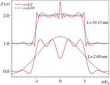
Figure 1: (Color online) Wigner function for two sizes $L$ computed at two points $x$ indicated in the legend. Gold’s Fermi wave vector $p_{F}/\hbar=12$ nm^-1 is used.

One might think that one could use the WF as if it were a distribution function in cases where its shape resembles a Fermi distribution. Let us inspect the curves for $f(x,P)$ computed as indicated above and presented in Fig. 1. In fact, at smaller sizes (close to the linear size of the DG’s Au₁₃-clusters DelaneyGreer:04a ) the WF does not bear much resemblance to a Fermi function (the lower curves of Fig. 1), At larger sizes (much larger than those one could hope to tackle within ab initio calculations to correlated molecules, for which the DG approach DelaneyGreer:04a was conceived) the curves (the upper part of Fig. 1) become more similar to a step function, and one may think that this is encouraging. In reality, the contrary is true: as visible in Fig. 1, mathematically one can calculate the WF for positive and negative “momentum” variables $P$ separately. However, this mathematical separation does not reflect a physical reality: for any single-particle eigenstate $\kappa$ the electron momentum vanishes, $P_{\kappa}\equiv-i\hbar\int d\,x\phi_{\kappa}^{\ast}(x)\left(\partial/\partial x\right)\phi_{\kappa}(x)=0$; left- and right-traveling waves are entangled with equal weight, and one cannot speak of single-particle eigenstates representing left- or right-moving electrons only because Wigner functions with positive or negative $P$-arguments can be computed. This represents a further limitation of the usefulness of the WF, not related to the Heisenberg’s principle, which is particularly relevant for transport. The current has a direction, and if one wants to unambiguously specify this direction, the WF $f(x,P)$ is inappropriate; a WF with negative (positive) “momentum”, $P<0$ ($P>0$), does not imply that left- and right-moving particles exist in the real physical world.

So, using $f(q_{L},P>0)$ and $f(q_{R},P<0)$ as if they were true momentum distributions of incoming electrons, as DG did,DelaneyGreer:04a is not justified in quantum mechanics. The above example demonstrates that, indeed, the textbook’s warning mentioned in the beginning of this section is pertinent.

IX Why any approach to transport merely based on a finite isolated cluster necessarily fails

In the course of our extensive critical investigations Baldea:2008b ; Baldea:2009c ; Baldea:2010g ; Baldea:unpublished of the DG approach DelaneyGreer:04a we became aware of a series of difficulties, which not only the DG’s but also other approaches to nanotransport are faced with, which we want to bring to the reader’s attention.

To understand the problem, let us briefly consider the uncorrelated dot model of Ref. Baldea:2008b, linked to semi-infinite electrodes ($M_{L,R}\to\infty$). Exact transport calculations at arbitrary bias $V$ can be easily carried out within a multitude of approaches.Blandin:76 ; Brako:85 ; Medvedev:05 ; Baldea:2010e Besides the current $J$ and dot occupancy $N_{0}$,Blandin:76 ; Brako:85 ; Medvedev:05 ; Baldea:2010e the occupancies of the sites in electrodes can also be computed.Baldea:unpublished

In Fig. 2, we present steady-state results for the electron number on the dot $N_{0}$ and that for nanoclusters $N_{c}$ centered on the dot and including several electrodes’ sites $N_{s}$. As visible there, the changes in both $V$ (source-drain voltage) and $\varepsilon_{g}$ (gate potential) yield variations in the dot occupancy $N_{0}$. (Notice that there is no exchange of electrons with the gate.) The total number $N_{c}$ of electrons in the nanoclusters also varies, it closely follows the change of $N_{0}$; the variations in the small difference $N_{c}-N_{0}$ could be hardly seen within the drawing accuracy of Fig. 2, and therefore are not shown there. The fact that $N_{c}-N_{0}$ is practically constant implies that the sites in electrodes remain practically unaffected by changes in $V$ and $\varepsilon_{g}$; even the electrodes’ sites in the very close dot’s vicinity are very little affected. The dependence $N_{c}\equiv N_{c}(V,\varepsilon_{g})$ is most important in the context of a transport approach. It demonstrates that, by varying $V$ and/or $\varepsilon_{g}$, a finite nanocluster exchanges electrons with the infinite electrodes linked to it, which act as reservoirs that can supply/withdraw electrons.

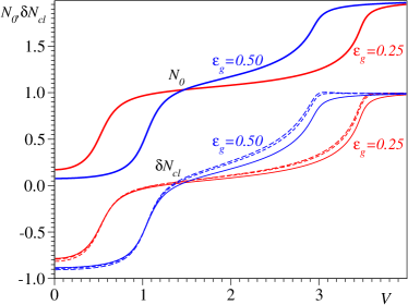
Figure 2: (Color online) Dot charge $N_{0}$ and cluster excess charge $\delta N_{cl}=N_{c}-N_{s}$ for two gate potentials $\varepsilon_{g}=0.5$ ($N_{s}=3,9,11$) and $\varepsilon_{g}=0.25$ ($N_{s}=3,11,13$). For both gate potentials, the employed cluster sizes $N_{s}$ given in parentheses increase upwards for, say, $V\sim 3$. Notice that for larger sizes the excess charge rapidly saturates and closely follows the dot charge, and this gives a flavor on how fast the convergence to charge neutrality within more distant parts of electrodes is (see the main text). Energy unit is $\mathcal{T}_{L,R}=1$ and $\tau_{L,R}=0.2$.

In the light of the aforementioned, it becomes clear that it is strictly impossible to correctly describe the transport within a DG-like approach, which considers a small isolated cluster. Within an approach like that initiated by DG DelaneyGreer:04a and further scrutinized by us Baldea:2008b ; Baldea:2009c ; Baldea:2010g one attempts to describe the transport using such a cluster characterized by a many-electron wave function $\Psi(x_{1},x_{2},\ldots,x_{N})$ to be determined by a constrained minimization of cluster’s energy for $V\neq 0$. This wave function merely describes a nanocluster with a given number of electrons $N$, which cannot be varied by changing source-drain ($V$) or gate ($\varepsilon_{g}$) voltages:

• whatever the property chosen to be constrained (WF, electron momentum distribution or else),

• whatever the boundary conditions (oBC, pBCs, Moebius, general twisted or else) which might be chosen for the finite “electrodes” included in the cluster (the Au₁₃-clusters of Ref. DelaneyGreer:04a, ),

• let the many-electron wave function $\Psi(x_{1},x_{2},\ldots,x_{N})$ be determined within exact full CI expansions (i. e, using the whole Hilbert space) as done by us Baldea:2008b ; Baldea:2009c ; Baldea:2010g and not only approximately, by using a reduced number of configurations selected by Monte-Carlo sampling, as DG did.DelaneyGreer:04a

Even the most “carefully” chosen constraints can at most, e. g., acceptably account for the change the number of electrons in the device (dot). But this change will inevitably modify the charge of the neighboring sites in electrodes. It is easy to imagine how profound will be the impact on the transport, e. g, in correlated or switchable devices. It is hard to conceive that the transport could be reasonably described within this framework, even if the cluster would be very large (what is obviously hard within the presently available ab initio quantum-chemical calculations for correlated systems): because it is by no way obvious/necessary that the local charge density be incorrectly described only at the remote ends of the finite “electrodes”, which would allow to suppose/hope that the electric field within the device will be little affected. A further difficulty is, of course, the fact that the number of electrons $N_{c}(V,\varepsilon_{g})$ of the coupled nanocluster is generally noninteger (cf. Fig. 2), but we do not discuss this issue here.Baldea:unpublished

One may further ask whether a “careful” choice of a certain charge state of the dot (molecule) instead of the neutral species could help. No, it does not. For the above model, one can also compute the exact time-dependent dot population $N_{0}(t)$ by suddenly coupling at $t=0$ a dot with population $N_{0}(0)$ to infinite electrodes.Brako:85 ; Blandin:76 ; Medvedev:05 The result for $V\neq 0$ within the wide band limit ($4\mathcal{T}\gg V,\varepsilon_{g},\Gamma$, where $\Gamma\equiv 2\tau^{2}/\mathcal{T}$, $\mathcal{T}=\mathcal{T}_{L}=\mathcal{T}_{R}$, and $\tau=\tau_{L}=\tau_{R}$) is Baldea:unpublished

$$N_{0}(t) = N_{0}(0)e^{-2\Gamma t}+\left(1+e^{-2\Gamma t}\right)$$

$$\times\left[1-\frac{1}{\pi}\left(\arctan\frac{2\varepsilon_{g}+eV}{2\Gamma}+\arctan\frac{2\varepsilon_{g}-eV}{2\Gamma}\right)\right]$$

$$-\frac{2\Gamma}{\pi}e^{-\Gamma t}\left(\int_{-\infty}^{-\varepsilon_{g}-eV/2}+\int_{-\infty}^{-\varepsilon_{g}+eV/2}\right)d\,\varepsilon\ \frac{\cos(\varepsilon t)}{\varepsilon^{2}+\Gamma^{2}}.$$

Figure 3: (Color online) Curves for the time-dependent dot charge $N_{0}(t)$ showing that the asymptotic values do not keep track of the initial occupancy $N_{0}(0)$. The values of the source-drain bias $V$, energy offset $\varepsilon_{g}$, and hybridisation $\Gamma$ are given in the legend.

As seen in Fig. 3, which visualizes the result expressed by Eq. (IX), the asymptotic value of the dot population $\lim_{t\to\infty}N(t)$, which corresponds to the steady state, does not “remember” the initial value $N(0)$; it is determined by the applied voltages.

The foregoing analysis makes it also clear that not only a variational ansatz like the DG’s is incorrect. The above list (a) – (c) can be enlarged by stating that, whatever the ansatz (let it be a variational ansatz better than the DG’s or based on e. g., Liouville Frensley:90 or Schrödinger equations) used to compute the wave function for a fixed $N$, it will fail. The aforementioned flaw is serious and can be unambiguously traced back to the use of a finite (small) isolated cluster. Electric transport can only occur in an open system, and allowing electron exchange with environment (infinite electrodes) is indispensable. Most commonly, this is done via the embedding self-energies within the Keldysh-NEGF-approach,Datta:97 which enable the nanocluster to change the number of electrons it contains.

X Conclusion

Most important for the present Reply, we have demonstrated above that the DG’s claims of the Comment are incorrect and our critique of I is untouched.

The unphysical current ($J=0$) obtained in I is the result of the DG defective ansatz and by no means emerges from pretended unsuitable constraints of real orbitals, as DG incorrectly claim. Using complex orbitals does not in the least change the unphysical prediction of the DG variational ansatz; furthermore, it confirms more directly its incorrectness. In fact, the complex orbitals given by DG represents nothing but a particular case of the general case considered in I, for which our demonstration holds. For completeness, we have worked out this case in detail to explicitly specify the labels of the incoming charge carriers (not necessarily electrons), to demonstrate that they can be constrained without concomitantly constraining the outgoing carriers, and to show that the distribution of the outgoing carrieres represents the outcome of transport calculations. Of course, fully consistent with the unphysical prediction $J=0$, the distribution of the outgoing carriers deduced within the defective DG ansatz is found equal to that of the incoming carriers.

To conclude, DG concede that our idea of constraining populations “is an interesting alternative to the Wigner function”, but argue that it is essential for this to choose complex states. We have shown above that the usage of the complex orbitals just of the form indicated by them as key point of a way-out solution does not mender the DG variational approach. These are not only complex, they are just of the form $\alpha_{\kappa}^{DG}(x)=\exp(i\kappa x)$, which DG give (and incorrectly attempt to suggest that they used them in Ref. DelaneyGreer:04a, ). Consequently, they must now accept that their variational ansatz for transport is incorrect.

The analysis done in conjunction with the issues raised by DG has led us to reveal two aspects of more general relevance for the transport theory. First, we have presented an example illustrating a limitation of the Wigner function $f(x,P)$ important for transport, namely that the sign of $P$ is not necessarily related to the direction of motion in the real world. Second, we have presented an important physical reason why transport approaches, which, like the DG’s, use information pertaining to a finite isolated cluster are inappropriate. This enlarges the basis of our critique recently formulated in Sec. VII of Ref. Baldea:2010g, , where two other fundamental reasons were exposed.

To summarize our detailed investigations on the DG approach,DelaneyGreer:04a we can state that this approach lamentably fails because virtually all its ingredients are incorrect:

• The DG approach imposes boundary conditions as if the WF were a true particle distribution, which is not justified quantum mechanically. Replacing the WF-constraints by the boundary conditions most justified physically (namely, the Fermi distributions) attempted in I does not remedy this approach.

• Even if the WF were a true momentum distribution, by uncritically constraining $f(q_{L},P>0)$ and $f(q_{R},P<0)$ it is very possible to erroneously constrain the outgoing majority charge carriers and not incoming ones. (This is just the case in Refs. DelaneyGreer:04a, ; DelaneyGreer:04b, ; DelaneyGreer:06, .)

• The DG approach attempts to describe the transport by using a finite cluster within calculations based on a variational principle (entropy maximization), which turned out to be problematic even if, unlike in the DG case, the limits of infinite time and infinite volume are taken in the correct order.Bokes:03 ; Baldea:2010g

• The DG approach aims at describing the transport by means of a wave function determined for a (small) isolated cluster, whose number of electrons is fixed, while a nanocluster in a real electric circuit does exchange electrons with the infinite electrodes to which it is connected.

The lamentable failure of the DG approach was demonstrated by explicit calculations for the simplest uncorrelated and correlated, discrete and continuous models.Baldea:2008b ; Baldea:2010g They contradict well-established experimental and theoretical results, and it would make little sense to more amply document the incorrectness in many other cases.Baldea:unpublished By contrast, DG could not present even a single example where it is valid.

Based on ingredients unfounded physically, it is not at all surprising that the currents predicted by the DG approach are completely unphysical and much poorly agreeing with experiment that more common approaches, contrary to the seemingly original success claimed in Ref. DelaneyGreer:04a, . In Sec. VIII of Ref. Baldea:2010g, , we clearly showed that a standard NEGF-DFT calculation yields currents slightly larger by a factor $\sim 1.5-3$, while DG’s currents DelaneyGreer:04a represent $\sim 2-5$% of the experimental currents of the recent accurate experiment of Ref. Reed:09, .

References

- (1) P. Delaney and J. C. Greer, Comment on “Critical analysis of a variational method used to describe molecular electron transport”, 2010.
- (2) I. Bâldea and H. Köppel, Phys. Rev. B 80, 165301 (2009).
- (3) P. Delaney and J. C. Greer, Phys. Rev. Lett. 93, 036805 (2004).
- (4) I. Bâldea and H. Köppel, Phys. Rev. B 78, 115315 (2008).
- (5) I. Bâldea and H. Köppel, Phys. Rev. B 82, 087302 (2010).
- (6) I. Bâldea (unpublished).
- (7) I. Bâldea and H. Köppel, Phys. Rev. B 80, 209902 (2009).
- (8) I. Bâldea, H. Köppel, and L. S. Cederbaum, J. Phys. Soc. Jpn. 68, 1954 (1999).
- (9) W. R. Frensley, Rev. Mod. Phys. 62, 745 (1990).
- (10) H. Song, Y. Kim, Y. H. Jang, H. Jeong, M. A. Reed, and T. Lee, Nature 462, 1039 (2009).
- (11) P. Delaney and J. C. Greer, Int. J. Quant. Chem. 100, 1163 (2004).
- (12) P. Delaney and J. C. Greer, Proc. Roy. Soc. A 462, 117 (2006).
- (13) I. Bâldea, H. Köppel, and L. S. Cederbaum, Eur. Phys. J. B 20, 289 (2001).
- (14) G. D. Mahan, Many-Particle Physics, Plenum Press, New York and London, second edition, 1990.
- (15) S. Datta, Electronic Transport in Mesoscopic Systems, Cambridge Univ. Press, Cambridge, 1997.
- (16) A. Blandin, A. Nourtier, and D. Hone, J. Phys. France 37, 369 (1976).
- (17) R. Brako and D. M. Newns, Rep. Prog. Phys. 52, 655 (1989).
- (18) I. G. Medvedev, Russ. J. Electrochem. 41, 227 (2005).
- (19) I. Bâldea and H. Köppel, Phys. Rev. B 81, 193401 (2010).
- (20) P. Bokes and R. W. Godby, Phys. Rev. B 68, 125414 (2003).