Mapping between long-time molecular and Brownian dynamics
Abstract
We use computer simulations to test a simple idea for mapping between long-time self diffusivities obtained from molecular and Brownian dynamics. The strategy we explore is motivated by the behavior of fluids comprising particles that interact via inverse-power-law pair potentials, which serve as good reference models for dense atomic or colloidal materials. Based on our simulation data, we present an empirical expression that semi-quantitatively describes the “atomic” to “colloidal” diffusivity mapping for inverse-power-law fluids, but also for model complex fluids with considerably softer (star-polymer, Gaussian-core, or Hertzian) interactions. As we show, the anomalous structural and dynamic properties of these latter ultrasoft systems pose problems for other strategies designed to relate Newtonian and Brownian dynamics of hard-sphere-like particles.
Computer simulations and statistical mechanical theories have long served as invaluable tools for understanding relaxation processes that occur in fluid systems that range from molecular liquids to complex suspensions of Brownian particles. Likos (2001) Depending on the resolution of the interparticle interactions used to model these systems, some descriptions of the microscopic dynamics are more appropriate to adopt than others. Simplistically, Newtonian (i.e., classical molecular) dynamics (MD) is suitable when the particles of interest are described by force fields with molecular-scale resolution. Modeling the motion of suspended Brownian particles, on the other hand, typically calls for coarser interparticle forces and dynamics that approximately account for the effects of the solvent. Löwen (1994); Ermak (1975); Brady and Bossis (1985); Hoogerbrugge and Koelman (1992); Malevanets and Kapral (1999)
Although the short-time behavior of a given model depends sensitively on its microscopic dynamics,Heyes and Brańka (1994) there is evidence that under certain conditions–e.g., dense fluids near the glass transition–the qualitative long-time behavior is largely independent of those details.Löwen et al. (1991); Gleim et al. (1998) With this in mind, it is perhaps not surprising that researchers often select the type of microscopic dynamics to use in simulations based on other considerations, such as computational efficiency. A common example is adopting classical MD to explore the long-time dynamic behavior of model complex fluids with coarse, effective interactions, ignoring the kinetic role of the implicit “fast” degrees of freedom, e.g, solvent.Stillinger and Weber (1978); Foffi et al. (2002); Puertas et al. (2003); Mausbach and May (2006); Moreno and Likos (2007); Krekelberg et al. (2009a); Pamies et al. (2009); Pond et al. (2009); Berthier et al. (2010) Although the qualitative trends provided by these MD simulations have been valuable, there is still the question of how to map between the long-time MD data of such simulations and that which would have been produced assuming a different type of microscopic dynamics.
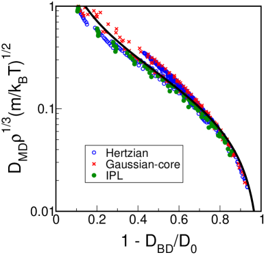
Here, we take a first step toward addressing this issue. Specifically, we present computer simulation results that test a simple heuristic approach for mapping between long-time self-diffusion coefficients obtained from Newtonian and Brownian (i.e., overdamped Langevin) dynamics (BD). The method follows from a seemingly naive hypothesis that “what matters” in such a mapping can be deduced from the behavior of a fluid of particles that interact via an inverse-power-law (IPL) pair potential [], where , is the interparticle separation, and represent characteristic energy and length scales of the interaction, and determines the steepness of the IPL repulsion. The IPL model is a natural reference system for dense atomic or colloidal fluids, whose static and dynamic properties are dominated by the repulsive part of their interactions. Furthermore, one can showRosenfeld (1977); Hoover (1991); Gnan et al. (2009) that a one-to-one relation must exist between the following dimensionless representations of the long-time diffusivities of an IPL fluid associated with the two types of dynamics: and . Here, is the number density, is the particle mass, is the Boltzmann constant, and is temperature. () represents the long-time self diffusivity obtained from MD (BD) trajectories, respectively, and is the value of in the dilute () limit. Based on previous work,Rosenfeld (1999); Lange et al. (2009); Pond et al. (2011a) it is clear that the relationship between and for IPL fluids is approximately independent of for . Hence, a more precise statement of our aforementioned hypothesis is that the quasi-universal IPL mapping relationship can also be used to estimate from (or vice versa) for other types of fluids, perhaps including those with very different types of interactions and physical properties.
To test this hypothesis, we carry out MD and BD simulations that probe the long-time dynamics of fluids of particles that interact via IPL potentials with , , , , and . We also explore the behavior of fluids with particles interacting via ultrasoft Gaussian-coreStillinger (1976) [, HertzianPamies et al. (2009) [], and effective star-polymerLikos et al. (1998) [ for , and for ] potentials. Here, , , and is the star polymer arm number. The latter three model systems have received considerable attention recently in the theoretical soft matter literature,Likos (2001); Foffi et al. (2003); Pamies et al. (2009) and represent stringent test cases for our approach (and others) due to their distinctive dynamical trends; e.g., each exhibits a wide range of conditions where self diffusivity anomalously increases with increasing particle density, as opposed to the behavior of IPL fluids. The MD and BD simulations that we present here cover much of the computationally accessible phase space of these model fluids, including both equilibrium and moderately supercooled conditions ( state points in total). As we show below, a potentially useful outcome of our analysis of this extensive data set is an empirical analytical equation that semi-quantitatively relates and for these systems.
The MD simulations of our study generate dynamic trajectories by solving Newton’s equation of motion using the velocity-Verlet algorithm in the microcanonical ensemble.Allen and Tildesley (1987) For IPL, Hertzian, and star-polymer fluids, they contain particles (, , and respectively) and use integration time steps of , and 0.001 , respectively. The BD simulations presented here generate trajectories by solving the Langevin equation in the high-friction limit using the conventional Brownian (Ermak) algorithm.Allen and Tildesley (1987); Ermak (1975) For the star-polymer fluid, they contain particles, and use a time step of where and . All simulations use a periodically replicated cubic cell with reduced volume determined by the number density of interest. For the IPL, Hertzian, and star-polymer systems, the pair potentials are truncated at (depending on )Pond et al. (2011a), and respectively. Long-time tracer diffusivities from both MD and BD simulation trajectories are computed from the average mean-squared particle displacements via the Einstein relation. For the analysis presented below, we also include some previously reported MD simulation dataKrekelberg et al. (2009a) for the Gaussian-core fluid and BD simulation dataPond et al. (2011a) for the IPL, Gaussian-core, and Hertzian fluids. The methods used in those studies are the same as those described above, and the required simulation parameters can be found in the original papers.
Before examining the simulation data of the various model fluids discussed above, we first consider what should generally be expected about the relationship between the dimensionless diffusivities, and . For example, to leading order in , we know that and , which together imply that in this limit. Furthermore, there is also evidenceLöwen et al. (1991); Gleim et al. (1998) suggesting that for supercooled liquids near the glass transition (, ). Since necessarily shows pronounced variations with small changes in or under these latter conditions, we also have . The following expression,
| (1) |
is an example of a simple heuristic functional form that interpolates between the aforementioned characteristic “fast” and “slow” limiting behaviors. Below, we examine how well eq. 1 can describe the simulation data for a variety of fluids comprising hard to ultrasoft particles if and are treated as constants.
Computer simulation data of plotted versus for the IPL, Gaussian-core, and Hertzian fluids are presented in Fig. 1. The data span the plane (details in the caption), characterizing the relationship between MD and BD long-time diffusivities for these fluids in their equilibrium and moderately supercooled states. Also presented in Fig. 1 is a least-squares fit of the data using the form provided by eq. 1. As can be seen–despite the distinctive non-monotonic dynamic trends of the Gaussian-core and Hertzian fluids as a function of densityMausbach and May (2006); Wensink et al. (2008); Krekelberg et al. (2009a); Wensink et al. (2008); Pamies et al. (2009); Krekelberg et al. (2009b); Pond et al. (2011a) –the data qualitatively behave as the equation predicts. In fact, as is illustrated in Fig. S1, more than 98% of the simulation data for for each of these model fluids are within 20% of the eq. 1 estimation based on the simulated . Furthermore, to the extent that the data shown in Fig. 1 reflect quasi-universal behavior, it suggests that the well-known, empirical dynamic freezing criterion for colloidal fluids (),Löwen et al. (1993) has an analog in atomic systems ().
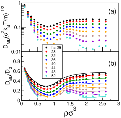
As an illustration of how eq. 1 might be further used, we consider the star-polymer fluidLikos et al. (1998) mentioned above. The soft, logarithmic repulsive interactions of this model are known to produce highly non-monotonic dynamic trends; e.g., diffusivity show two minima as a function of (see Fig. 2 of this paper and Fig. 1 of Foffi et al. Foffi et al. (2003)). When a model fluid displays such nontrivial behavior with one type of microscopic dynamics (e.g., MD), it is not obvious a priori whether the trends will necessarily be reflected when another type (e.g., BD) is employed. In fact, an earlier investigation of this systemFoffi et al. (2003) made a point to report dynamic results from both types of simulations. What Fig. 2b illustrates that is that one can, to a very good approximation, predict for this system by simply substituting its data of panel Fig. 2a into eq. 1 with no adjustable parameters (i.e., using and from data in Fig. 1, which did not include the star-polymer fluid). As is illustrated in Fig. S1, the predicted values for 88% of the state points are within 20% of the simulation results.
We are not aware of another mapping approach that can make predictions of similar accuracy for both hard and ultrasoft particle fluids. One alternative strategy,de Schepper et al. (1989); Pusey et al. (1990); Cohen and de Schepper (1991); Lopez-Flores et al. (2011) hypothesizes that , where . Although this relationship approximately holds for simple fluids with steep repulsions (the so-called hard-sphere dynamic universality class),Lopez-Flores et al. (2011) we show that it breaks down qualitatively for fluids with ultrasoft interactions. Specifically, Fig. S2 illustrates that predictions based on this hypothesis for the star-polymer system are generally very inaccurate–except for a narrow region of phase space with extremely low and high –where particle overlaps are avoided.
Note that a quantitative link between and is easy to establish for models where both can be expressed as single-valued functions of the same static quantity. For example, one can showGnan et al. (2009) that, for an IPL fluid, and are strictly single-valued functions of excess entropy (relative to ideal gas), . In fact, the same is approximately true for other simple liquids that are “strongly correlating” and mimic a variety of static and dynamic properties of IPL systems.Gnan et al. (2009)
Do Gaussian-core, Hertzian, and star-polymer fluids show excess-entropy scaling behaviors similar to the IPL fluids? To check this, we compute for these models using free-energy-based simulation methods. Specifically, we determine the density dependence of the Helmholtz free energy at high temperature using grand canonical transition-matrix Monte Carlo simulation.Errington (2003) We then carry out canonical temperature-expanded ensemble simulationsLyubartsev et al. (1992) with a transition-matrix Monte Carlo algorithmGrzelak and Errington (2010) to calculate the change in Helmholtz free energy with temperature at constant density. Together, these simulations provide the excess Helmholtz free energy and excess energy, and hence . Additional details on these simulations can be found elsewhere in our earlier papers.Chopra et al. (2010); Pond et al. (2011b)
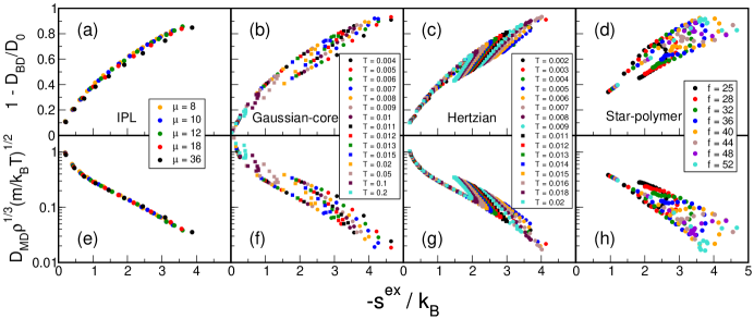
The excess entropy scaling behaviors of and are plotted in Fig. 3 for all model fluids and state points shown in Fig. 1 and 2. The main point is that, in stark contrast to the behavior of the IPL fluids, and of the ultrasoft fluids are not (even approximately) single-valued functions of . Hence, the success of the IPL-motivated mapping strategy between MD and BD diffusivities reported here cannot be explained by appealing to arguments about strongly-correlating fluids.
As a final note, we emphasize that this mapping has yet to be tested for systems with structural and dynamic properties that are strongly influenced by attractive interactions, a class of fluids that we plan to investigate in the near future.
T.M.T. acknowledges support of the Welch Foundation (F-1696) and the National Science Foundation (CBET-1065357). J. R. E. acknowledges financial support of the National Science Foundation (CBET-0828979). M.J.P. acknowledges the support of the Thrust 2000 - Harry P. Whitworth Endowed Graduate Fellowship in Engineering. The Texas Advanced Computing Center (TACC), the University at Buffalo Center for Computational Research, and the Rensselaer Polytechnic Institute Computational Center for Nanotechnology Innovations provided computational resources for this study.
References
- Likos (2001) C. N. Likos, Phys. Rep. 348, 267 (2001).
- Löwen (1994) H. Löwen, Phys. Rep. 237, 249 (1994).
- Ermak (1975) D. L. Ermak, J. Chem. Phys. 62, 4189 (1975).
- Brady and Bossis (1985) J. F. Brady and G. Bossis, J. Fluid Mech. 155, 105 (1985).
- Hoogerbrugge and Koelman (1992) P. J. Hoogerbrugge and J. M. V. A. Koelman, Europhys. Lett. 19, 155 (1992).
- Malevanets and Kapral (1999) A. Malevanets and R. Kapral, J. Chem. Phys 110, 8605 (1999).
- Heyes and Brańka (1994) D. Heyes and A. Brańka, Physics and Chemistry of Liquids 28, 95 (1994).
- Löwen et al. (1991) H. Löwen, J.-P. Hansen, and J.-N. Roux, Phys. Rev. A 44, 1169 (1991).
- Gleim et al. (1998) T. Gleim, W. Kob, and K. Binder, Phys. Rev. Lett. 81, 4404 (1998).
- Stillinger and Weber (1978) F. H. Stillinger and T. A. Weber, J. Chem. Phys. 68, 3837 (1978).
- Foffi et al. (2002) G. Foffi, K. A. Dawson, S. V. Buldyrev, F. Sciortino, E. Zaccarelli, and P. Tartaglia, Phys. Rev. E 65, 050802(R) (2002).
- Puertas et al. (2003) A. M. Puertas, M. Fuchs, and M. E. Cates, Phys. Rev. E 67, 031406 (2003).
- Mausbach and May (2006) P. Mausbach and H. O. May, Fluid Phase Equilib. 249, 17 (2006).
- Moreno and Likos (2007) A. J. Moreno and C. N. Likos, Phys. Rev. Lett. 99, 107801 (2007).
- Krekelberg et al. (2009a) W. P. Krekelberg, T. Kumar, J. Mittal, J. R. Errington, and T. M. Truskett, Phys. Rev. E 79, 031203 (2009a).
- Pamies et al. (2009) J. Pamies, A. Cacciuto, and D. Frenkel, J. Chem. Phys. 131, 044514 (2009).
- Pond et al. (2009) M. J. Pond, W. P. Krekelberg, V. K. Shen, J. R. Errington, and T. M. Truskett, J. Chem. Phys. 131, 161101 (2009).
- Berthier et al. (2010) L. Berthier, A. J. Moreno, and G. Szamel, Phys. Rev. E 82, 060501 (2010).
- Rosenfeld (1977) Y. Rosenfeld, Phys. Rev. A 15, 2545 (1977).
- Hoover (1991) W. G. Hoover, Computational Statistical Mechanics (Elsevier Science Pub Co, 1991), pp. 172–173.
- Gnan et al. (2009) N. Gnan, T. B. Schrøder, U. R. Pedersen, N. P. Bailey, and J. C. Dyre, J. Chem. Phys. 131, 234504 (2009).
- Rosenfeld (1999) Y. Rosenfeld, J. Phys.: Condens. Matter 11, 5415 (1999).
- Lange et al. (2009) E. Lange, J. B. Caballero, A. M. Puertas, and M. Fuchs, J. Chem. Phys 130, 174903 (2009).
- Pond et al. (2011a) M. J. Pond, J. R. Errington, and T. M. Truskett, J. Chem. Phys 134, 081101 (2011a).
- Stillinger (1976) F. H. Stillinger, J. Chem. Phys. 65, 3968 (1976).
- Likos et al. (1998) C. N. Likos, H. Löwen, M. Watzlawek, B. Abbas, O. Jucknischke, J. Allgaier, and D. Richter, Phys. Rev. Lett. 80, 4450 (1998).
- Foffi et al. (2003) G. Foffi, F. Sciortino, P. Tartaglia, E. Zaccarelli, F. L. Verso, L. Reatto, K. A. Dawson, and C. N. Likos, Phys. Rev. Lett. 90, 238301 (2003).
- Allen and Tildesley (1987) M. P. Allen and D. J. Tildesley, Computer Simulations of Liquids (Oxford University Press, New York, 1987).
- Wensink et al. (2008) H. Wensink, H. Löwen, M. Rex, C. Likos, and S. van Teeffelen, Comput. Phys. Commun. 179, 77 (2008).
- Krekelberg et al. (2009b) W. Krekelberg, M. Pond, G. Goel, V. Shen, J. Errington, and T. Truskett, Phys. Rev. E 80, 61205 (2009b).
- Löwen et al. (1993) H. Löwen, T. Palberg, and R. Simon, Phys. Rev. Lett. 70, 1557 (1993).
- de Schepper et al. (1989) I. M. de Schepper, E. G. D. Cohen, P. N. Pusey, and H. N. W. Lekkerkerker, J. Phys.: Condens. Matter 1, 6503 (1989).
- Pusey et al. (1990) P. Pusey, H. Lekkerkerker, E. Cohen, and I. de Schepper, Physica A 164, 12 (1990).
- Cohen and de Schepper (1991) E. G. D. Cohen and I. M. de Schepper, J. Stat. Phys. 63, 241 (1991).
- Lopez-Flores et al. (2011) L. Lopez-Flores, P. Mendoza-Mendez, L. E. Sanchez-Diaz, G. Perez-Angel, M. Chavez-Paez, A. Vizcarra-Rendon, and M. Medina-Noyola, arXiv:1106.2475v1 (2011).
- Errington (2003) J. R. Errington, J. Chem. Phys. 118, 9915 (2003).
- Lyubartsev et al. (1992) A. P. Lyubartsev, A. A. Martsinovski, S. V. Shevkunov, and P. N. Vorontsov-Velyaminov, J. Chem. Phys. 96, 1776 (1992).
- Grzelak and Errington (2010) E. M. Grzelak and J. R. Errington, Langmuir 26, 13297 13304 (2010).
- Chopra et al. (2010) R. Chopra, T. M. Truskett, and J. R. Errington, J. Phys. Chem. B 114, 10558 (2010).
- Pond et al. (2011b) M. J. Pond, J. R. Errington, and T. M. Truskett, arXiv:1107.4996 (2011b).
![[Uncaptioned image]](/html/1108.1038/assets/x4.png)
Figure S1. Ratio of long-time BD diffusivity estimated from eq. 1 in the text, , to that obtained from simulation, , plotted as a function of . The dashed red lines represent a 20% deviation of the predicted diffusivity from the value measured in simulation.
![[Uncaptioned image]](/html/1108.1038/assets/x5.png)
Figure S2. Long-time diffusivity of the star-polymer system from MD and BD simulations. Symbols are the same as in Figure 2 of the main text. Curves in panel (b) show prediction based on , where Lopez-Flores et al. (2011).